Imaging Thermal Anomalies in Hot Dry Rock Geothermal Systems from Near-Surface Geophysical Modelling

 , , , ,
  , , and
Abstract
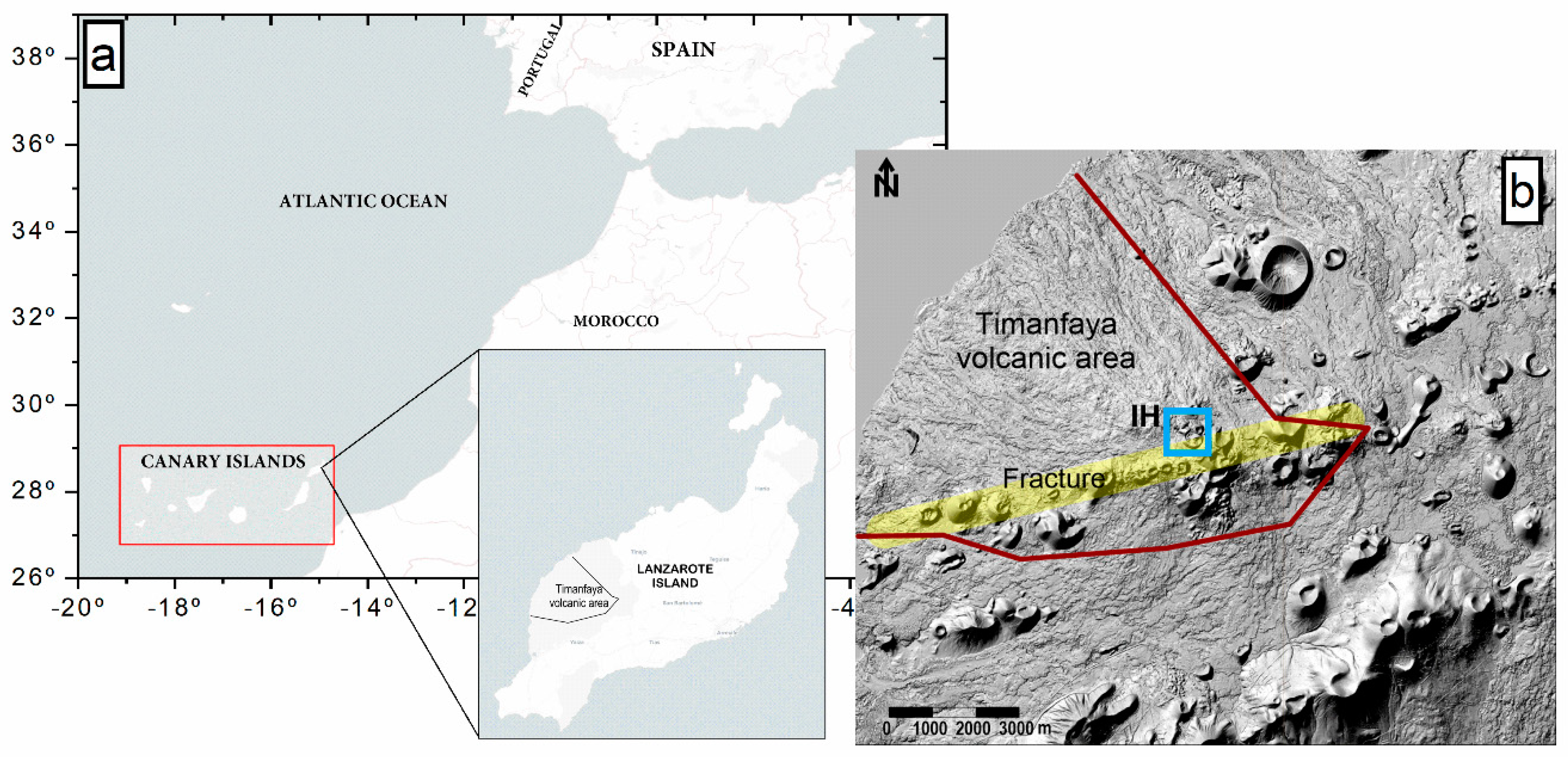
1. Introduction
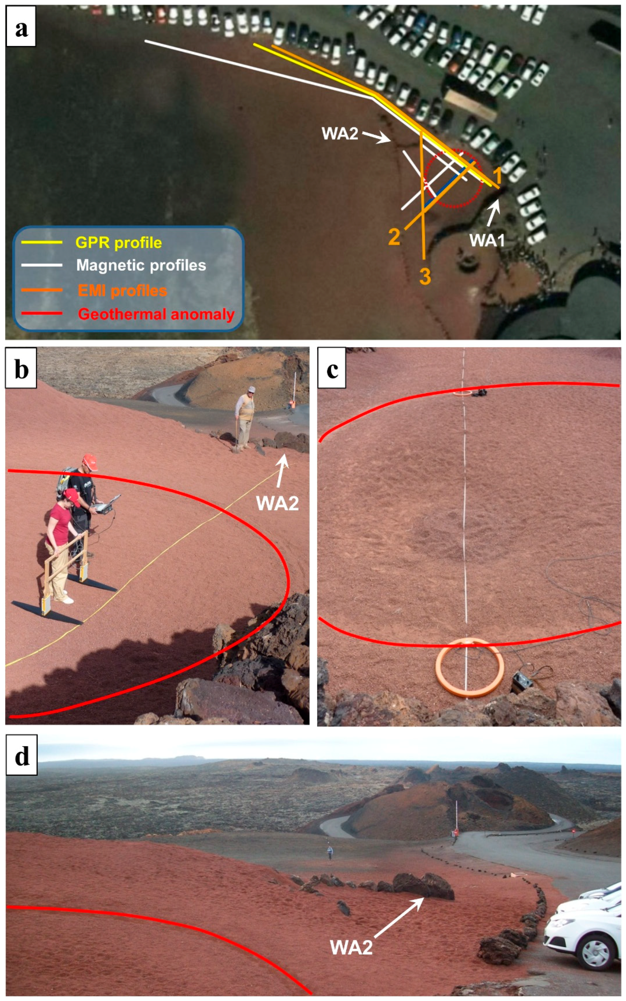
2. Geophysical Techniques
2.1. Ground Penetrating Radar (GPR)
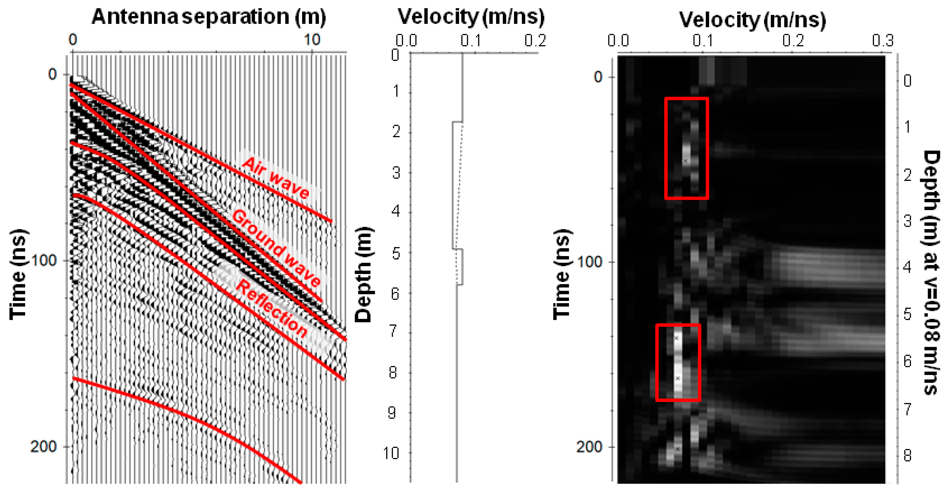
GPR Data Acquisition and Processing
2.2. Electromagnetic Survey
2.3. Magnetic Survey
Magnetic Data Processing and Rock Magnetic Properties
3. Results
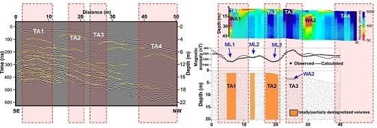
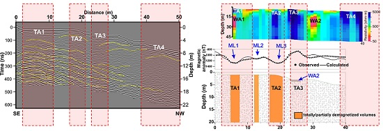
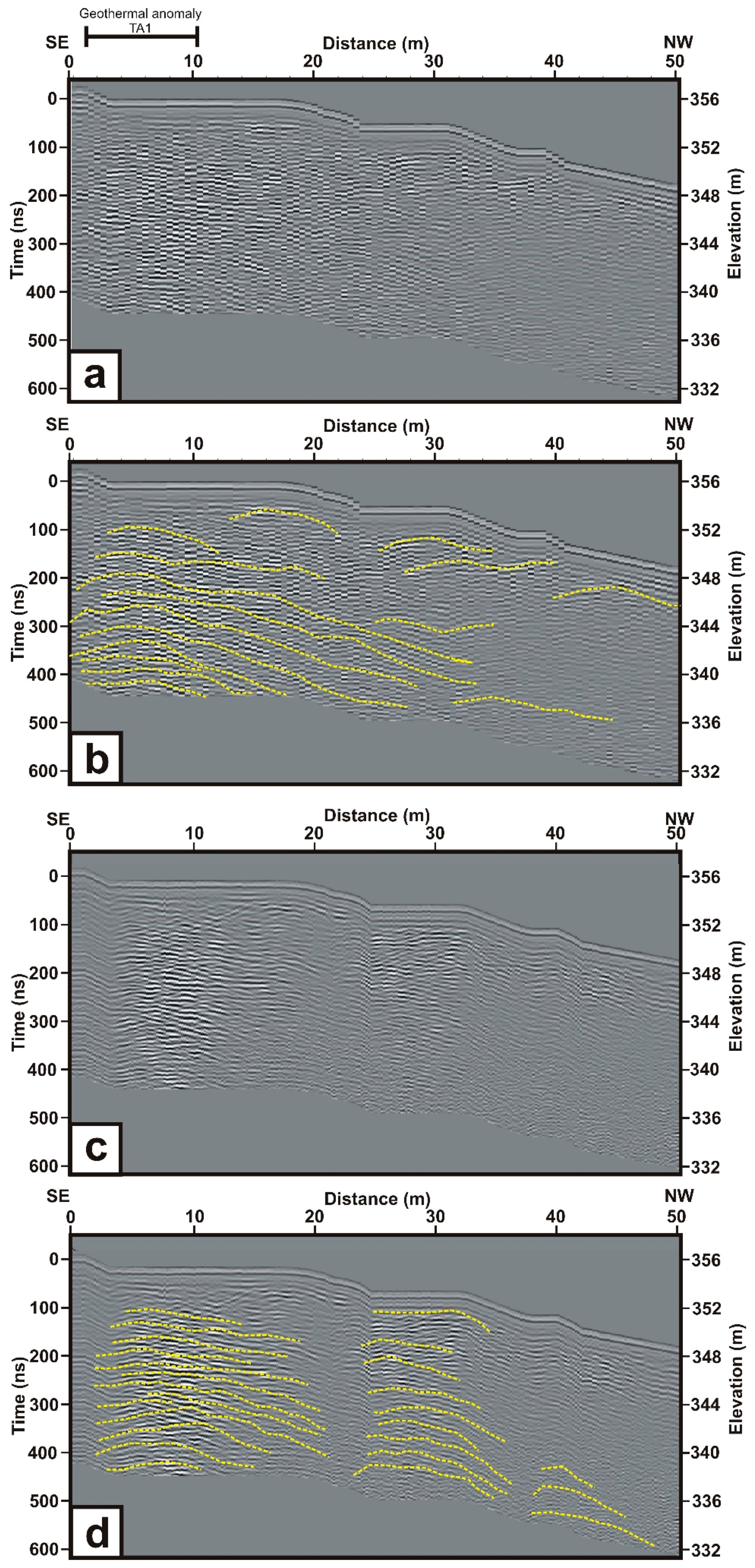
3.1. GPR Results
3.2. EMI Results
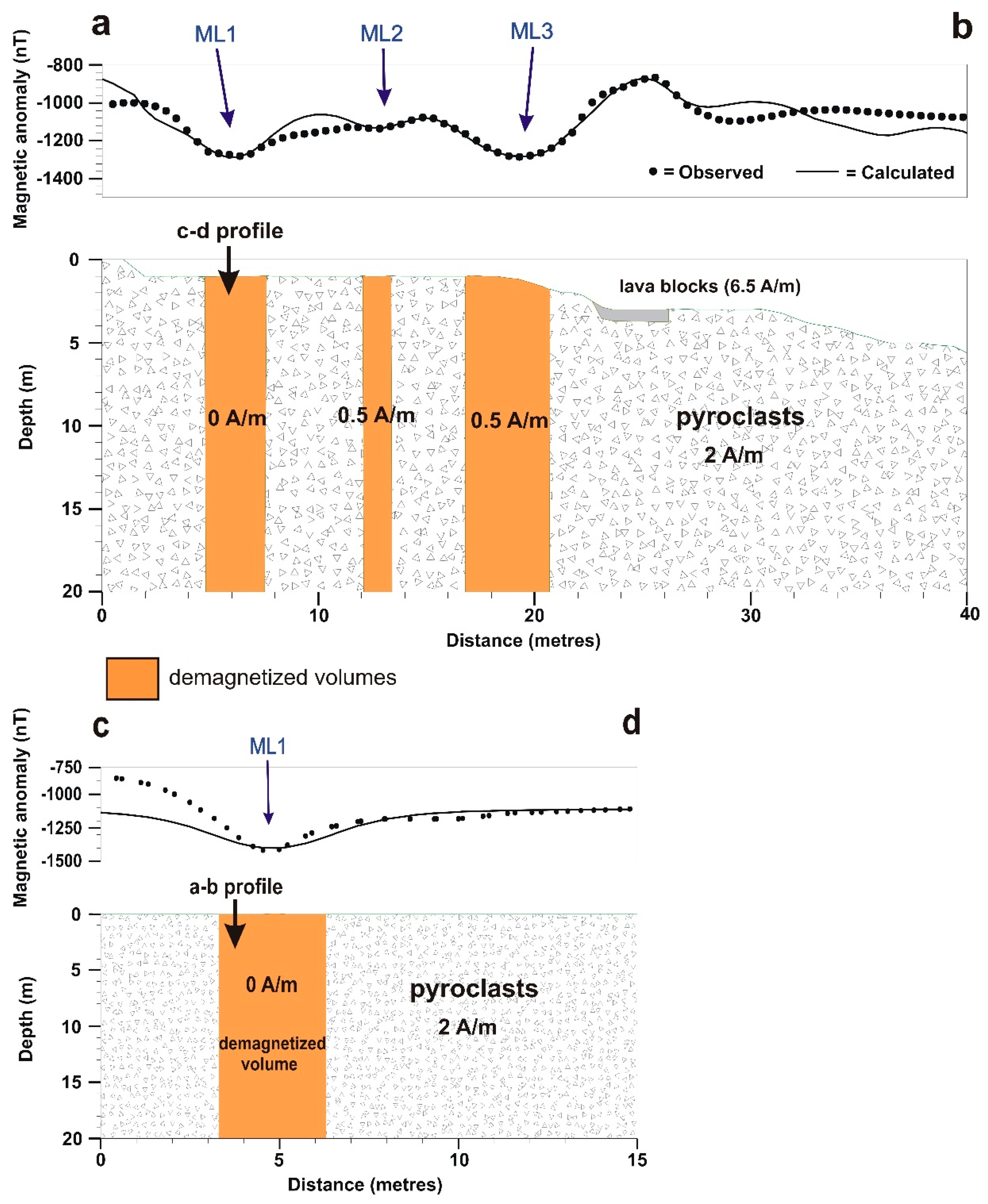
3.3. Magnetic Modelling Results
4. Discussion
4.1. Relation between GPR Signal and Ground Temperature
4.2. Seasonal Temperature Variations from the GPR Signal
4.3. Relation between Resistivity Anomalies and Ground Temperature
4.4. Relation between Magnetic Anomalies and Ground Temperature
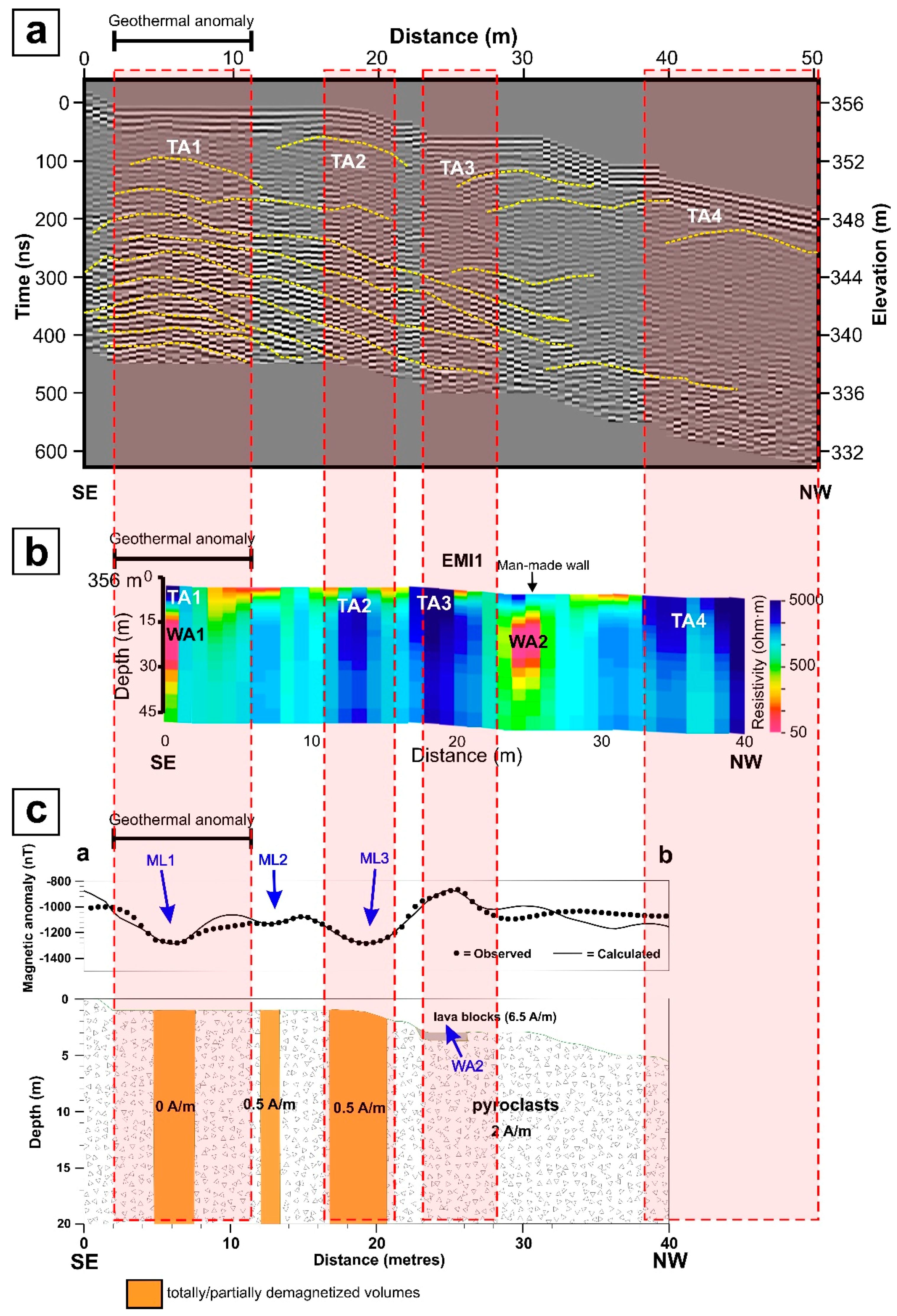
4.5. Joint Interpretation of GPR, EMI and Magnetic Data for the Detection of Shallow Geothermal Anomaly Areas
5. Conclusions
Author Contributions
Funding
Acknowledgments
Conflicts of Interest
References
- Muñoz, G. Exploring for Geothermal Resources with Electromagnetic Methods. Surv. Geophys. 2014, 35, 101–122. [Google Scholar] [CrossRef]
- DiPippo, R.; Renner, J.L. Geothermal Energy. In Future Energy, 2nd ed.; Letcher, T.M., Ed.; Elsevier: Waltham, MA, USA, 2014; pp. 211–223. [Google Scholar]
- Brown, D.W.; Duchane, D.V.; Heiken, G.; Hriscu, V.T. Mining the Earth’s Heat: Hot Dry Rock Geothermal Energy; Springer: Berlin/Heidelberg, Germany, 2012; p. 658. [Google Scholar]
- Coello, J.; Cantagrel, J.M.; Hernán, F.; Fúster, J.M.; Ibarrola, B.; Ancochea, E.; Casquet, C.; Jamond, C.; Díaz de Terán, J.R.; Cendrero, A. Evolution of the eastern volcanic ridge of the Canary Islands based on new K-Ar data. J. Volcanol. Geoth. Res. 1992, 53, 251–274. [Google Scholar] [CrossRef]
- Romero, C. La Erupción de Timanfaya (Lanzarote-1730–1736). Análisis Documental y Estudio Geomorfológico; Secretariado de Publicaciones de la Universidad de La Laguna, La Laguna: Tenerife, Spain, 1991; p. 136. [Google Scholar]
- Carracedo, J.C.; Rodríguez Badiola, E.R.; Soler, V. The 1730–1736 eruption of Lanzarote: An unusually long, high magnitude fissural basaltic eruption in the recent volcanism of the Canary Islands. J. Volcanol. Geoth. Res. 1992, 53, 239–250. [Google Scholar] [CrossRef]
- Ortiz, R.; Araña, V.; Astiz, M.; García, A. Magnetotelluric study of the Teide (Tenerife) and Timanfaya (Lanzarote) volcanic areas. J. Volcanol. Geoth. Res. 1986, 30, 357–377. [Google Scholar] [CrossRef]
- Díez Gil, J.L.; Araña, V.; Ortiz, R.; Yuguero, J. Stationary convection model for heat transport by means of geothermal fluids in post eruptive systems. Geothermics 1987, 15, 77–87. [Google Scholar] [CrossRef]
- Carracedo, J.C.; Troll, V. The Geology of Canary Islands; Elsevier: Amsterdam, The Netherlands, 2016; p. 621. [Google Scholar]
- Albert, J.F.; Diez Gil, J.L.; Valentin, M.A.; Torres, F. Evaluación de las anomalías geotérmicas de Lanzarote. In Serie Casa de los Volcanes; Garcia, A., Felpeto, A., Eds.; Servicio de publicaciones del Excmo, Cabildo Insular de Lanzarote: Lanzarote, Spain, 1994; Volume 3, pp. 41–60. [Google Scholar]
- Araña, V.; Díez Gil, J.L.; Ortiz, R.; Yuguero, J. Convection of geothermal fluids in the Timanfaya volcanic area (Lanzarote, Canary Islands). Bull. Volcanol. 1984, 47, 667–677. [Google Scholar] [CrossRef]
- García, A. Estudio magnetotelúrico del área volcánica de Timanfaya (Lanzarote). Anal. Fis. Ser. B 1986, 35–43. [Google Scholar]
- García, A. Modelos Corticales a Partir de Sondeos Magnetotelúricos. Aplicación a Zonas Volcánicas Activas. Master’s Thesis, University Complutense of Madrid, Madrid, Spain, 1983. [Google Scholar]
- Annan, P. GPR Principles, Procedures & Applications; Sensors and Software Inc.: Mississauga, ON, Canada, 2003; p. 278. [Google Scholar]
- Daniels, D.J. Ground Penetrating Radar; The institution of Electrical Engineers: London, UK, 2004; p. 726. [Google Scholar]
- Jol, H.M. Ground Penetrating Radar: Theory and Applications; Elsevier Science: Amsterdam, The Netherlands, 2009; p. 544. [Google Scholar]
- Sandmeier, K.J. ReflexW Version 8.5. Windows™ XP/7/8/10-program for the processing of seismic, acoustic or electromagnetic reflection, refraction and transmission data; Sandmeier: Karsruhe, Germany, 2018; p. 327. [Google Scholar]
- Tosti, F.; Slob, E. Determination, by using GPR, of the volumetric water content in structures, substructures, foundations and soils. In Civil Engineering Applications of Ground Penetrating Radar; Benedetto, A., Pajewski, L., Eds.; Springer: New Delhi, India, 2015; pp. 163–194. [Google Scholar]
- Aziz, Z.; van Geen, A.; Stute, M.; Versteeg, R.; Horneman, A.; Zheng, Y.; Goodbred, S.; Steckler, M.; Weinman, B.; Gavrieli, I.; et al. Impact of local recharge on arsenic concentrations in shallow aquifers inferred from the electromagnetic conductivity of soils in Araihazar, Bangladesh. Water Resour. Res. 2008, 44, 2007WR006000. [Google Scholar] [CrossRef]
- Paine, J.G. Determining salinization extent, identifying salinity sources, and estimating chloride mass using surface, borehole, and airborne electromagnetic induction methods. Water Resour. Res. 2003, 39, 1–10. [Google Scholar] [CrossRef]
- Everett, M.E.; Meju, M.A. Near-surface controlled-source electromagnetic induction: Background and recent advances. In Hydrogeophysics; Rubin, Y., Hubbard, S.S., Eds.; Springer: New York, NY, USA, 2005; pp. 157–183. [Google Scholar]
- Bobee, C.; Schmutz, M.; Camerlynck, C.; Robain, H. An integrated geophysical study of the western part of the Rochechouart-Chassenon impact structure, Charente, France. Near Surf. Geophys. 2010, 4, 259–270. [Google Scholar] [CrossRef]
- Valois, R.; Camerlynck, C.; Dhemaied, A.; Guerin, R.; Hovhannissian, G.; Plagnes, V.; Rejiba, F.; Robain, H. Assessment of doline geometry using geophysics on the Quercy plateau karst (South France). Earth Surf. Process. 2011, 36, 1183–1192. [Google Scholar] [CrossRef]
- McNeill, J.D. Electromagnetic Terrain Conductivity Measurement at Low Induction Numbers; Technical Note TN-6; Geonics Ltd.: Mississauga, ON, Canada, 1980; p. 15. [Google Scholar]
- UBC-GIF, 2000. EM1DFM: A Program Library for Forward Modelling and Inversion of Frequency Domain Electromagnetic Data over 1D Structures. 2000. Available online: https://em1dfm.readthedocs.io/en/latest/ (accessed on 22 January 2019).
- Farquharson, C.G.; Oldenburg, D.W.; Rough, P.S. Simultaneous 1D inversion of loop-loop electromagnetic data for magnetic susceptibility and electrical conductivity. Geophysics 2003, 68, 1857–1869. [Google Scholar] [CrossRef]
- Hunt, C.P.; Moskowitz, B.M.; Banerjee, S.K. Magnetic properties of rocks and minerals. In Rock Physics and Phase Relations, A Handbook of Physical Constants; Ahrens, T.J., Ed.; American Geophysical Union: Washington, DC, USA, 1995; Volume 3, pp. 189–204. [Google Scholar]
- Hildenbrand, T.G.; Rosenbaum, J.G.; Kauahikaua, J.P. Aeromagnetic study of the island of Hawaii. J. Geophys. Res. 1993, 98, 4099–4119. [Google Scholar] [CrossRef]
- Blanco, I.; García, A.; Torta, J.M. Magnetic study of the Furnas caldera (Azores). Ann. Geophys. 1997, 40, 341–359. [Google Scholar]
- Hoechstein, M.P.; Soengkono, S. Magnetic anomalies associated with high temperature reservoirs in the Taupo Volcanic Zone (New Zealand). Geothermics 1997, 26, 1–24. [Google Scholar] [CrossRef]
- Caratori Tontini, F.; de Ronde, C.E.J.; Scott, B.J.; Soengkono, S.; Stagpoole, V.; Timm, C.; Tivey, M. Interpretation of gravity and magnetic anomalies at Lake Rotomahana: Geological and hydrothermal implications. J. Volcanol. Geoth. Res. 2016, 314, 84–94. [Google Scholar] [CrossRef]
- Paoletti, V.; Passaro, S.; Fedi, M.; Marino, C.; Tamburrino, S.; Ventura, G. Sub-circular conduits and dikes offshore the Somma-Vesuvius volcano revealed by magnetic and seismic data. Geophys. Res. Lett. 2016, 43, 9544–9551. [Google Scholar] [CrossRef]
- Finlay, C.C.; Maus, S.; Beggan, C.D.; Bondar, T.N.; Chambodut, A.; Chernova, T.A.; Chulliat, A.; Golovkov, V.P.; Hamilton, B.; Hamoudi, M.; et al. International Geomagnetic Reference Field: The eleventh generation. Geophys. J. Int. 2010, 183, 1216–1230. [Google Scholar]
- Baranov, V. A New Method for Interpretation of Aeromagnetic Maps, Pseudo-Gravimetric Anomalies. Geophysics 1957, 22, 359–363. [Google Scholar] [CrossRef]
- Calvo-Rathert, M.; Morales-Contreras, J.; Carrancho, A.; Gogichaishvili, A. A comparison of Thellier-type and multispecimen paleointensity determinations on Pleistocene and historical flows from Lanzarote (Canary Islands, Spain). Geochem. Geophys. Geosyst. 2016, 17, 3638–3654. [Google Scholar] [CrossRef]
- Conyers, L.B. Ground-Penetrating Radar for Archaeology; AltaMira Press: Walnut Creek, CA, USA, 2004; p. 203. [Google Scholar]
- Olhoeft, G.R. Electrical, magnetic, and geometric properties that determine ground penetrating radar performance. In Proceedings of the 7th International Conference on Ground Penetrating Radar (GPR’98), Lawrence, KS, USA, 27–30 May 1998; pp. 477–483. [Google Scholar]
- Valentín, A. La Fase Gaseosa Relacionada con la Actividad Volcánica y Tectónica. Master’s Thesis, University of Barcelona, Barcelona, Spain, 1988. [Google Scholar]
- Riccardi, U.; Arnoso, J.; Benavent, M.; Vélez, E.; Tammaroe, U.; Montesinos, F.G. Exploring deformation scenarios in Timanfaya volcanic area (Lanzarote, Canary Islands) from GNSS and ground based geodetic observations. J. Volcanol. Geoth. Res. 2018, 357, 14–24. [Google Scholar] [CrossRef]
- Pettinelli, E.; Beaubien, S.E.; Lombardi, S.; Annan, A.P. GPR, TDR, and geochemistry measurements above an active gas vent to study near surface gas-migration pathways. Geophysics 2008, 73, A11–A15. [Google Scholar] [CrossRef]
- Dougherty, A.J.; Lynne, B.Y. A novel geophysical approach to imagine sinter deposits and other subsurface geothermal features utilizing ground penetrating radar. Geoth. Res. Trans. 2010, 34, 857–863. [Google Scholar]
- Dougherty, A.J.; Lynne, B.Y. Utilizing Ground Penetrating Radar and Infrared Thermography to Image Vents and Fractures in Geothermal Environments. Geoth. Res. Trans. 2011, 35, 743–750. [Google Scholar]
- Hersir, G.P.; Björnsson, A. Geophysical Exploration for Geothermal Resources, Principles and Application; UNU-GTP, report 15: Reykjavik, Iceland, 1991; p. 94. [Google Scholar]
- Spichak, V.; Manzella, A. Electromagnetic Sounding of Geothermal Zones. J. Appl. Geophys. 2009, 68, 459–478. [Google Scholar] [CrossRef]
- Börner, J.H.; Bär, M.; Spitzer, K. Electromagnetic methods for exploration and monitoring of enhanced geothermal systems—A virtual experiment. Geothermics 2015, 55, 78–87. [Google Scholar] [CrossRef]
- Spichak, V.; Zakharova, O.; Goidina, A. A new conceptual model of the Icelandic crust in the Hengill geothermal area based on the indirect electromagnetic geothermometry. J. Volcanol. Geoth. Res. 2013, 257, 99–112. [Google Scholar] [CrossRef]
- Lumb, J.T.; Macdonald, W.J.P. Near-surface resistivity surveys of geothermal areas using the electromagnetic method. Geothermics 1970, 2, 311–317. [Google Scholar] [CrossRef]
- Risk, G.F.; Caldwell, T.G.; Bibby, H.M. Tensor time domain electromagnetic resistivity measurements at Ngatamariki geothermal field, New Zealand. J. Volcanol. Geoth. Res. 2003, 127, 33–54. [Google Scholar] [CrossRef]
- Simpson, M.P.; Bignall, G. Undeveloped high-enthalpy geothermal fields of the Taupo Volcanic Zone, New Zealand. Geothermics 2016, 59, 325–346. [Google Scholar] [CrossRef]
- Gailler, L.S.; Bouchot, V.; Martelet, G.; Thinon, I.; Coppo, N.; Baltassat, J.M.; Bourgeois, B. Contribution of multi-method geophysics to the understanding of a high-temperature geothermal province: The Bouillante area (Guadeloupe, Lesser Antilles). J. Volcanol. Geoth. Res. 2014, 275, 34–50. [Google Scholar] [CrossRef]
- Spichak, V.; Zakharova, O. Constructing the Deep Temperature Section of the Travale Geothermal Area in Italy, with the use of an Electromagnetic Geothermometer. Izv. Phys. Solid Earth 2015, 51, 87–94. [Google Scholar] [CrossRef]
- Rodríguez, F.; Pérez, N.M.; Padrón, E.; Melián, G.; Piña-Varas, P.; Dionis, S.; Barrancos, J.; Padilla, G.D.; Hernández, P.A.; Marrero, R.; et al. Surface geochemical and geophysical studies for geothermal exploration at the southern volcanic rift zone of Tenerife, Canary Islands, Spain. Geothermics 2015, 55, 195–206. [Google Scholar] [CrossRef]
- Roberts, J.J.; Duba, A.G.; Bonner, B.P.; Kasameyer, P.W. The effects of capillarity on electrical resistivity during boiling in metashale from scientific corehole SB-15-D, The Geysers, California, USA. Geothermics 2001, 30, 235–254. [Google Scholar] [CrossRef]
- Hochstein, M.P.; Hunt, T.M. Seismic, gravity and magnetic studies, Broadlands geothermal field, New Zealand. Geothermics 1970, 2, 333–346. [Google Scholar] [CrossRef]
- Soengkono, S. Magnetic anomalies over the Ngatamariki Geothermal Field, Taupo Volcanic Zone, New Zealand. In Proceedings of the 14th New Zealand Geothermal Workshop, University of Auckland, New Zealand, 4–6 November 1992; pp. 241–246. [Google Scholar]
- Gómez-Ortiz, D.; Montesinos, F.; Martín-Crespo, T.; Solla, M.; Arnoso, J.; Vélez, E. Combination of geophysical prospecting techniques into areas of high protection value: Identification of shallow volcanic structures. J. Appl. Geophys. 2014, 109, 15–26. [Google Scholar] [CrossRef]
- Byrdina, S.; Vandemeulebrouck, J.; Cardellini, C.; Legaz, A.; Camerlynckc, C.; Chiodini, G.; Lebourg, T.; Gresse, M.; Bascoua, P.; Motos, G.; et al. Relations between electrical resistivity, carbon dioxide flux, and self-potential in the shallow hydrothermal system of Solfatara (Phlegrean Fields, Italy). J. Volcanol. Geoth. Res. 2014, 283, 172–182. [Google Scholar] [CrossRef]
- Rinaldi, A.P.; Todesco, M.; Vandemeulebrouck, J.; Revil, A.; Bonafede, M. Electrical conductivity, ground displacement, gravity changes, and gas flow at Solfatara crater (Campi Flegrei caldera, Italy): Results from numerical modeling. J. Volcanol. Geoth. Res. 2011, 207, 93–105. [Google Scholar] [CrossRef]
- Chambefort, I.; Buscarlet, E.; Wallis, I.C.; Sewell, S.; Wilmarth, M. Ngatamariki Geothermal Field, New Zealand: Geology, geophysics, chemistry and conceptual model. Geothermics 2016, 59, 266–280. [Google Scholar] [CrossRef]
- Antoine, A.; Finizola, A.; Lopez, T.; Baratoux, D.; Rabinowicz, M.; Delcher, E.; Fontaine, F.R.; Fontaine, F.J.; Saracco, G.; Bachèlery, P.; et al. Electric potential anomaly induced by humid air convection within Piton de La Fournaise volcano, La Réunion Island. Geothermics 2017, 65, 81–98. [Google Scholar] [CrossRef]


| Step | Filter | Parameters |
|---|---|---|
| 1 | Time-zero correction | --- |
| 2 | Subtract-mean (dewow) | Time window: 10 ns |
| 3 | Energy decay | Scaling value: 0.5 |
| 4 | Subtracting average | Average traces: 100 |
| 5 | Band-pass (butterworth) | Low pass: 40 MHz; high pass: 150 MHz |
| 6 | Topographic correction | Velocity: 0.08 m/ns |
| Site and Lithology | Magnetic Susceptibility (SI) | Induced Magnetization (A/m) | Remanent Magnetization, NRM | Q | |||
|---|---|---|---|---|---|---|---|
| Intensity (A/m) | Declination (°) | Inclination (°) | α95 | ||||
| TM1 (lava flow 1) | 0.011 ± 0.007 | 0.35 ± 0.22 | 22.5 ± 14.8 | 331.8 | 63.4 | 24.3 | 64 |
| TM2 (lava flow 2) | 0.019 ± 0.018 | 0.58 ± 0.57 | 10.4 ± 4.1 | 346.0 | 52.9 | 11.9 | 18 |
| TM3 (lava flow 3) | 0.020 ± 0.014 | 0.62 ± 0.42 | 15.2 ± 9.3 | 2.8 | 59.2 | 8.9 | 24 |
| TM4 (lava flow 4) | 0.025 ± 0.013 | 0.78 ± 0.40 | 12.9 ± 1.5 | 321.4 | 62.3 | 22.4 | 17 |
© 2019 by the authors. Licensee MDPI, Basel, Switzerland. This article is an open access article distributed under the terms and conditions of the Creative Commons Attribution (CC BY) license (http://creativecommons.org/licenses/by/4.0/).
Share and Cite
Gomez-Ortiz, D.; Blanco-Montenegro, I.; Arnoso, J.; Martin-Crespo, T.; Solla, M.; Montesinos, F.G.; Vélez, E.; Sánchez, N. Imaging Thermal Anomalies in Hot Dry Rock Geothermal Systems from Near-Surface Geophysical Modelling. Remote Sens. 2019, 11, 675. https://doi.org/10.3390/rs11060675
Gomez-Ortiz D, Blanco-Montenegro I, Arnoso J, Martin-Crespo T, Solla M, Montesinos FG, Vélez E, Sánchez N. Imaging Thermal Anomalies in Hot Dry Rock Geothermal Systems from Near-Surface Geophysical Modelling. Remote Sensing. 2019; 11(6):675. https://doi.org/10.3390/rs11060675
Chicago/Turabian StyleGomez-Ortiz, David, Isabel Blanco-Montenegro, Jose Arnoso, Tomas Martin-Crespo, Mercedes Solla, Fuensanta G. Montesinos, Emilio Vélez, and Nieves Sánchez. 2019. "Imaging Thermal Anomalies in Hot Dry Rock Geothermal Systems from Near-Surface Geophysical Modelling" Remote Sensing 11, no. 6: 675. https://doi.org/10.3390/rs11060675
APA StyleGomez-Ortiz, D., Blanco-Montenegro, I., Arnoso, J., Martin-Crespo, T., Solla, M., Montesinos, F. G., Vélez, E., & Sánchez, N. (2019). Imaging Thermal Anomalies in Hot Dry Rock Geothermal Systems from Near-Surface Geophysical Modelling. Remote Sensing, 11(6), 675. https://doi.org/10.3390/rs11060675