Assessment of the X- and C-Band Polarimetric SAR Data for Plastic-Mulched Farmland Classification

Abstract

We present a classification of plastic-mulched farmland (PMF) and other land cover types using full polarimetric RADARSAT-2 data and dual polarimetric (HH, VV) TerraSAR-X data, acquired from a test site in Hebei, China, where the main land covers include PMF, bare soil, winter wheat, urban areas and water. The main objectives were to evaluate the outcome of using high-resolution TerraSAR-X data for classifying PMF and other land covers and to compare classification accuracies based on different synthetic aperture radar bands and polarization parameters. Initially, different polarimetric indices were calculated, while polarimetric decomposition methods were used to obtain the polarimetric decomposition components. Using these polarimetric components as input, the random forest supervised classification algorithm was applied in the classification experiments. Our results show that in this study full-polarimetric RADARSAT-2 data produced the most accurate overall classification (94.81%), indicating that full polarization is vital to distinguishing PMF from other land cover types. Dual polarimetric data had similar levels of classification error for PMF and bare soil, yielding mapping accuracies of 53.28% and 59.48% (TerraSAR-X), and 59.56% and 57.1% (RADARSAT-2), respectively. We found that Shannon entropy made the greatest contribution to accuracy in all three experiments, suggesting that it has great potential to improve agricultural land use classifications based on remote sensing.

1. Introduction

Mulching farmland with plastic films can effectively reduce soil moisture evaporation and improve the efficiency of water use. Therefore, plastic-mulched farmland (PMF) has become an important agricultural landscape in recent years [1]. Accurately monitoring changes to the PMF distribution pattern and area is relevant to both current and future agricultural management in order to meet the growing demand for high-quality, sustainable agriculture [2].

Mulching farmland with plastic films has a positive effect on agricultural productivity because it can raise soil temperature and keep soil moisture. However, residues of plastic film in fields are beginning to have a negative effect on agricultural environments. Clearly, such large areas of PMF will inevitably have an impact on the surface energy balance and will put further pressure on agricultural environments [3]. Therefore, accurate monitoring of spatial and temporal changes to PMF distributions is also very relevant to the study of environmental change.

Remote sensing encompasses large scales of observation. It provides a convenient way to analyze the distribution of ground objects on a large scale, making it a feasible approach for monitoring PMF to determine its scale of impact on the environment and climate. In recent years, several studies have carried out the mapping of PMF using remote sensing. Lu et al. [3] showed that the decision-tree classifier is an effective method for extracting PMF over large geographic areas from Landsat-5 TM data, making it feasible to map spatial-temporal dynamics of PMF. Picuno et al. [4] employed the parallelepiped method to extract mulched fields from Landsat TM imagery, as well as synthetic aperture radar (SAR) imagery to validate their detection accuracy. Levin et al. [5] claimed that white and transparent plastic-mulch films have three absorption peaks, centered on 1218 nm, 1732 nm, and 2313 nm wavelengths that are unaffected by dust, rinses, and other surface factors. Lanorte et al. [6] mapped agricultural plastic waste from Landsat 8 satellite images using the support vector machine method. Novelli et al. [7] compared the performance of the Sentinel-2 multi-spectral instrument and Landsat-8 operational land imager for greenhouse detection. Carvajal et al. [8] proposed an artificial intelligence neural network to detect greenhouses using QuickBird imagery. Agüera and Liu [9] proposed an algorithm to detect greenhouses based on QuickBird and IKONOS imagery. Hasituya et al. [10] used spectral and textural features of Landsat-8 operational land imagery to monitor PMF and obtained satisfactory results. Yang et al. [11] proposed a new plastic greenhouse index (PGI) based on spectral, sensitivity, and separability analyses of greenhouses using medium spatial resolution images. They examined the effectiveness and capability of the proposed PGI, showing that plastic greenhouses in Landsat Enhanced Thematic Mapper Plus images could be successfully detected using the PGI.

However, optical remote sensing data remain affected by fog, rain and snow, making it difficult to guarantee their quality. In contrast, SAR remote sensing can function throughout the day in all types of weather. SAR also can penetrate specific targets. Recently, SAR remote sensing has been widely used for crop identification. Rabiger et al. [12] used TerraSAR-X and RADARSAT-2 for crop classification and acreage estimation in Canada; they clearly demonstrated the potential of X-Band data for crop identification. Ma et al. [13] investigated the potential of multi-temporal polarimetric RADARSAT-2 data for crop classification in an urban/rural fringe area. Skakun et al. [14] assessed the efficiency of multi-temporal C-band RADARSAT-2 intensity and Landsat-8 surface reflectance satellite imagery for crop classification in the Ukraine. They explored different combinations of optical and SAR images, as well as SAR modes and polarizations, for a better discrimination of crops. Jiao et al. [15] assessed the accuracy of an object-oriented classification of polarimetric SAR (PolSAR) data to map and monitor crops using 19 RADARSAT-2 fine beam polarimetric (FQ) images of an agricultural area in northeastern Ontario, Canada. Sonobe et al. [16] applied the random forest (RF) classifier as well as the classification and regression tree (CART) to evaluate the potential of multi-temporal dual-polarimetric (dual-pol) TerraSAR-X data, on strip-map mode, for the classification of crop types. Li et al. [17] used RADARSAT-2 quad PolSAR and dual-pol TerraSAR-X data to monitor agriculture crop growth stages. They found that entropy, the mean eigenvector (λ) and differential reflectivity of both data had similar sensitivities to crop growth stages over their common coverage period.

In the research of monitoring PMF using SAR data, Hasituya et al. [18] and Lu et al. [19] did some studies, however the potential of multi-band multi-polarization SAR data in the extraction of PMF has not been fully explored. In this paper, we evaluate the outcome of using different SAR data for classifying PMF and other land cover types. High-resolution dual-pol X-band TerraSAR-X data, C-band dual-pol RADARSAT-2 data and full-polarimetric (full-pol) RADARSAT-2 data were used to explore classifications based on different bands and different SAR data. The organizational structure of this paper is as follows: Section 2 introduces the test site, field investigations, pol SAR decomposition principles and the methods used in this study; Section 3 presents the experimental results of the classification of PMF and other land use types and a discussion of the results while our conclusions are presented in Section 4.

2. Materials and Methods

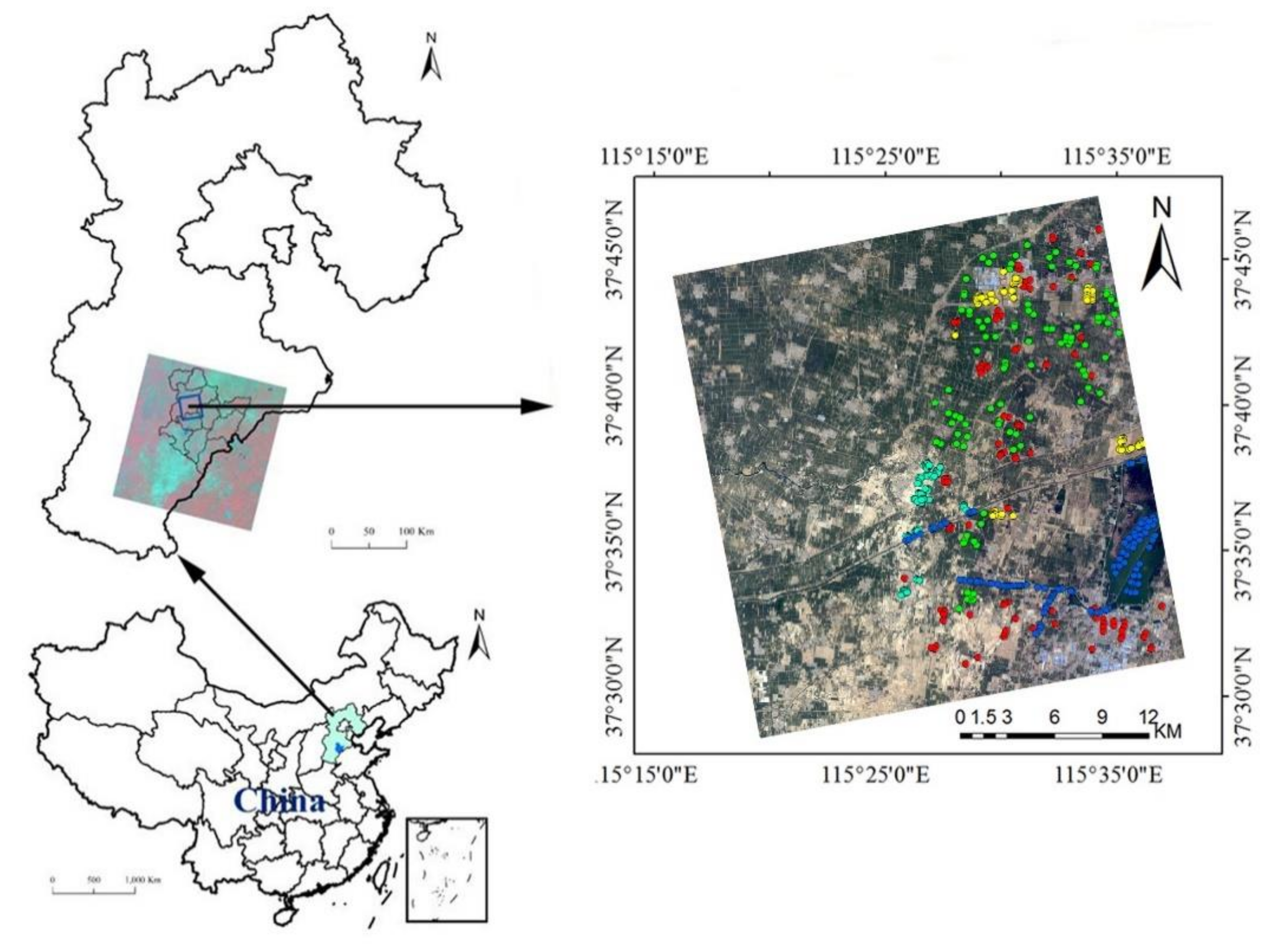
2.1. Test Site and Data

The experimentation area (115°15′–115°35′E, 37°30′–37°45′N; Figure 1) is situated in Jizhou, within the southeastern part of Hebei Province, China. The terrain is flat and open, forming a low plain, with an elevation of approximately 23–29 m and a total area of 8815 km². It has a semi-humid continental monsoon climate. The average annual temperature is 12–13 °C, and the frost-free period lasts approximately 170–220 days. The average annual precipitation is approximately 500–900 mm.

The main land use types are agricultural, where croplands have one or two crops a year. In addition to PMF, four land cover types cover the study area: winter wheat, bare soil, water and built-up areas. The main crop type in the study area is winter wheat, which comprises approximately 75% of the total agricultural land. Cotton is the main crop type in the areas covered with PMF and the phenological stage of it is emergence. The specific phenological periods of winter wheat are shown in

Table 1. The specific phenological periods of winter wheat in Jizhou.

Seeding Emergence Stage	Tillering Stage	Overwintering Period	Turning Green Stage	Jointing Stage	Heading and Flowering Stage	Milk Ripening Period	Mature Period
Early October–Middle October	Late October	Early December–Late December	Early March–Late March	Early April–Middle April	Late April–Early May	Middle May–Early Jun	Early Jun

.

RADARSAT-2 was launched in December 2007. This commercial radar satellite offers powerful technical options that enhance environmental monitoring, resource management and mapping worldwide. Full-pol RADARSAT-2 data were used for our analysis in ascending orbit, acquired on 3 May 2018. The incidence angle of the image was 26.6° and the pixel resolution was 4.73 m × 4.74 m (Azimuth × Range). The images have a swath of 25 km × 25 km.

Meanwhile, the German government and industries developed the TerraSAR-X radar satellite. It works within the X-band, with a central frequency of 9.6 GHZ. The data used in this study were dual copolarized (HH, VV) X-band SAR acquisitions of TerraSAR-X in descending orbit, because its quad-pol mode is still an experimental one and its acquisitions are not available to commercial users. The acquisition time of the data used for our classification experiment was 17 May 2018. The grid size of the geocoded images in this study was assigned to 3 m × 3 m. The incidence angle of the image was 33.75° and the swath of the image was 15 km × 50 km.

PolSARPro software (open source toolbox; European Space Agency, 2003) was used for the polarimetric analysis. The data were geometrically corrected using NEST software (The NEST Initiative, 2014). The Refined-Lee speckle filter with a 7 × 7 grid was applied to remove speckles.

2.2. Sampling

Apart from agricultural land, the two other common land cover types at the test site were urban and water areas. The urban area mainly consists of buildings, roads, and sparse vegetation. A ground quadrat of different ground classes was obtained using a global positioning system. The specific area depended on the natural boundary of the crop field. We collected ground sample data according to the satellite transition times. In the process of data collection, both systematic sampling and random sampling were adopted. After collecting field point samples, we digitized these polygon samples based on the location of field point samples on high spatial resolution (2 m) GF-1 satellite images. The samples were enlarged to polygon samples with a size of 30 m × 30 m. In total, 100 sample parcels were collected for each type, among them 70 were used for training and 30 were used for verification. Figure 1 shows the location of test site and the distribution of surface features on the GF-1 satellite image.

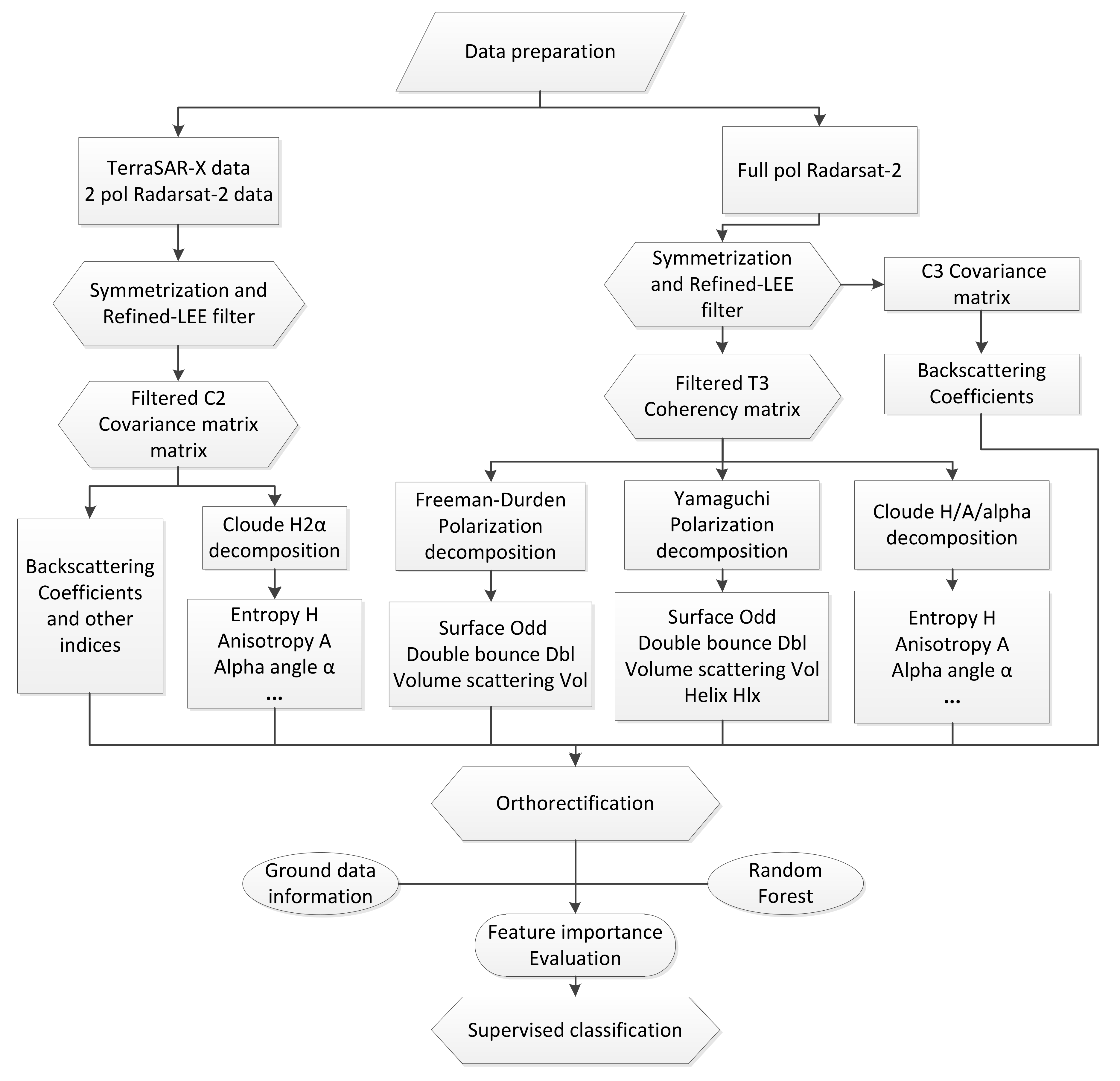
2.3. Principles and Methods

2.3.1. Dual Polarimetry and Its Scattering Parameters

We analyzed 26 dual-pol (HH, VV) parameters for the classification of PMF and other land cover types. These parameters are presented in

Table 2. Overview of the 26 parameters derived from the dual-polarimetric TerraSAR-X and RADARSAT-2 data.

Number	Parameter	Abbreviation
1	H-A-combination 1	HA
2	H-A-combination 2	H1mA
3	H-A-combination 3	1mHA
4	H-A-combination 4	1mH1mA
5	Probability 1	p1
6	Probability 2	p2
7	The mean eigenvector	lambda
8	The first eigenvector	l1
9	The second eigenvector	l2
10	Entropy_Shannon	SEdual
11	Entropy	Hdual
12	The mean scattering delta angle	delta
13	The first scattering delta angle	delta1
14	The second scattering delta angle	delta2
15	Anisotropy	Adual
16	The mean scattering alpha angle	alpha
17	The first scattering alpha angle	alpha1
18	The second scattering alpha angle	alpha2
19	The coherence amplitude	$\left|{\gamma }_{HHVV}\right|$
20	Backscattering coefficient of VV channel	${\mathsf{\sigma }}_{VV}$
21	HHVV phase difference	$\angle \langle S_{VV}{S}_{HH}^{*}\rangle$
22	Amplitude of $\langle S_{\mathrm{HH}}{S}_{\mathrm{VV}}^{*}\rangle$	$\left|\langle ,S_{VV}{S}_{HH}^{*},\rangle \right|$
23	Backscattering coefficient of HH channel	${\mathsf{\sigma }}_{HH}$
24	Backscattering coefficient ratio HH/VV	${\mathsf{\sigma }}_{HH/VV}$
25	Backscattering coefficient HH minus Backscattering coefficient of VV	${\mathsf{\sigma }}_{HH-VV}$
26	Backscattering coefficient HH plus Backscattering coefficient of VV	${\mathsf{\sigma }}_{HH+VV}$

.

In this study, the mathematical entropy/anisotropy/alpha (H/A/α) decomposition method proposed by Cloud and Pettier [20] was used to analyze the scattering mechanisms. The (H/A/$\mathsf{\alpha }$) quad-pol decomposition was later transferred by Cloude to an entropy/alpha (H2$\mathsf{\alpha }$) decomposition for dual-pol data [21]. For this study, we used the modified version of the (H2$\mathsf{\alpha }$) decomposition for the 2 × 2 Covariance matrix, [C₂], defined as follows, where v_i represent the characteristic vector of a matrix.

$$\langle \left[{\mathrm{C}}_2\right]\rangle =\left[\begin{array}{cc}\langle {\left|S_{XX}\right|}^2\rangle & \langle S_{XX}{S}_{YY}^{*}\rangle \\ \langle S_{YY}{S}_{XX}^{*}\rangle & \langle {\left|S_{YY}\right|}^2\rangle \end{array}\right]$$

(1)

$$\langle \left[{\mathrm{C}}_2\right]\rangle ={\displaystyle \sum }_{i=1}^2{\lambda }_i\underset{¯}{{\nu }_i} \underset{¯}{v_i^{T*}}={\lambda }_1{\left[{\mathrm{C}}_2\right]}_1+{\lambda }_2{\left[{\mathrm{C}}_2\right]}_2$$

(2)

We calculated different indices based on the HH and VV backscattering coefficients, as well as the dual-pol [C₂], including the coherence amplitude ($\left|{\gamma }_{HHVV}\right|$), backscattering coefficient of VV channel (${\mathsf{\sigma }}_{VV}$), HHVV phase difference ($\angle S_{VV}{S}_{HH}^{*}$), amplitude of $\langle S_{HH}{S}_{VV}^{*}\rangle$ ($\left|\langle ,S_{VV}{S}_{HH}^{*},\rangle \right|$), backscattering coefficient of the HH channel (${\mathsf{\sigma }}_{HH}$), backscattering coefficient ratio HH/VV (${\mathsf{\sigma }}_{HH/VV}$), backscattering coefficient of HH minus backscattering coefficient of VV (${\mathsf{\sigma }}_{HH-VV}$) and the backscattering coefficient HH plus backscattering coefficient of VV (${\mathsf{\sigma }}_{HH+VV}$).

According to the Cloude decomposition, each unitary eigenvector of the [C₂] may be parameterized using two real angular variables.

$$\underset{¯}{{\nu }_i}={\left[\cos {\alpha }_i,\sin {\alpha }_i{e}^{j{\delta }_i}\right]}^t$$

(3)

In this way, the estimate of the mean polarimetric parameter set is given by:

$$\left(\overline{\alpha },\overline{\delta }\right)={\displaystyle \sum }_{i=1}^2{p}_i\left({\alpha }_i,{\delta }_i\right)$$

(4)

Based on the modified Cloude decomposition of the [C₂], we obtained the eigenvalues l1 and l2 and their corresponding eigenvectors u1 and u2. The H-A-combination 1 (HA), H-A-combination 2 (H1mA), H-A-combination 3 (1mHA), H-A-combination 4 (1mH1mA), probability 2 (p2), probability 1 (p1), the mean eigenvector (λ), the second eigenvector (l2), the first eigenvector (l1), Shannon entropy (SE_dual), entropy (H_dual), the mean scattering delta angle (δ), the second scattering delta angle (δ2), the first scattering delta angle (δ1), anisotropy (A_dual), the mean scattering alpha angle (α), the second scattering alpha angle (α2) and the first scattering alpha angle (α1) were calculated using equations defined below.

Pseudo-probabilities of the [C₂] expansion elements are defined as:

$$p_i=\frac{{\lambda }_i}{{{\displaystyle \sum }}_{i=1}^2{\lambda }_i}=\frac{{\lambda }_i}{span}$$

(5)

The entropy (H) indicates the degree of statistical disorder of the scattering phenomenon:

$$H_{dual}={\displaystyle \sum }_{i=1}^2{p}_{i}lo{g}_3{p}_i$$

(6)

The anisotropy (A) is defined as the relative importance of the secondary scattering mechanisms:

$$A_{dual}=\frac{P_1-P_2}{P_1+P_2}$$

(7)

The dual-pol coherence between HH and VV channels is given by Equation (8), yielding a complex number. The coherence amplitude $\left|{\gamma }_{HHVV}\right|$ was used in this study [22].

$$\left|{\gamma }_{HHVV}\right|=\frac{\langle S_{VV}{S}_{HH}^{*}\rangle }{\sqrt{{\langle \left|S_{HH}\right|}^2\rangle \langle {\left|S_{VV}\right|}^2\rangle }}$$

(8)

SE_dual characteristic parameter of the H/α polarization decomposition is calculated using Equations (9)–(11), where Tr represents the trace of a matrix [23,24].

$$S{E}_{dual}=S{E}_I+S{E}_P$$

(9)

$$S{E}_I=2\log \left(\frac{\pi eTr\left[{\mathrm{C}}_2\right]}{2}\right)$$

(10)

$$S{E}_p=\log \left(4\frac{det\left[{\mathrm{C}}_2\right]}{Tr{\left[{\mathrm{C}}_2\right]}^2}\right)$$

(11)

2.3.2. Full Polarimetry and Its Scattering Parameters

Full-pol data contain all four polarization modes, which provide more information than dual-pol SAR data and can be used to analyze more complex scattering mechanisms. In this study, we analyzed 25 full-pol (HH, HV, VH and VV) parameters. These parameters are presented in

Table 3. Overview of the 25 parameters derived from the full-polarimetric RADARSAT-2 data.

Number	Parameter	Abbreviation
1	Yamaguchi_vol	Y_vol
2	Yamaguchi_odd	Y_odd
3	Yamaguchi_hlx	Y_hlx
4	Yamaguchi_dbl	Y_dbl
5	Probability 1	P1
6	Probability 2	P2
7	Probability 3	P3
8	The mean eigenvector	Lambda
9	The first eigenvector	l1
10	The second eigenvector	l2
11	The third eigenvector	l3
12	The gamma parameter	Gamma
13	Entropy_Shannon	SEfull
14	Entropy	Hfull
15	Double bounce Eigenvalue Relative Difference	Derd
16	The mean scattering delta angle	Delta
17	The beta parameter	Beta
18	Anisotropy	Afull
19	The mean scattering alpha angle	Alpha
20	Freeman_vol	F_vol
21	Freeman_odd	F_odd
22	Freeman_dbl	F_dbl
23	Backscattering coefficient of HV channel	${\mathsf{\sigma }}_{HV}$
24	Backscattering coefficient of VV channel	${\mathsf{\sigma }}_{VV}$
25	Backscattering coefficient of HH channel	${\mathsf{\sigma }}_{HH}$

.

We calculated different indices based on different polarimetric backscattering coefficients, including the backscattering coefficient of the HV channel (${\mathsf{\sigma }}_{HV}$), backscattering coefficient of the VV channel (${\mathsf{\sigma }}_{VV}$) and the backscattering coefficient of the HH channel (${\mathsf{\sigma }}_{HH}$).

For the full-pol data, the mathematically based entropy/anisotropy/alpha (H/A/α) decomposition proposed by Cloude and Pottier [20] was also selected for the scattering mechanisms analysis; it uses an eigenvalue/eigenvector analysis of the 3 × 3 Coherency matrix, [T₃], where v_i represent the characteristic vector of a matrix.

$${\mathrm{T}}_3=\left[\begin{array}{ccc}\langle \frac{1}{2}{\left|S_{HH}+S_{VV}\right|}^2\rangle & \langle \frac{1}{2}\left(S_{HH}+S_{VV}\right){\left(S_{HH}-S_{VV}\right)}^{*}\rangle & \left(\langle S_{HH}+S_{VV}\right)S_{HV}{}^{*}\rangle \\ \frac{1}{2}\langle {\left(S_{HH}+S_{VV}\right)}^{\ast }\left(S_{HH}-S_{VV}\rangle \right)& \langle \frac{1}{2}{\left|S_{HH}-S_{VV}\right|}^2\rangle & \langle \left(S_{HH}-S_{VV}\right)S_{HV}{}^{*}\rangle \\ \langle {\left(S_{HH}+S_{VV}\right)}^{*}{S}_{HV}\rangle & \langle {\left(S_{HH}-S_{VV}\right)}^{*}{S}_{HV}\rangle & \langle 2{\left|S_{HV}\right|}^2\rangle \end{array}\right]$$

(12)

$$\langle \left[{\mathrm{T}}_3\right]\rangle ={\displaystyle \sum }_{i=1}^3{\lambda }_i\underset{¯}{{\nu }_i} \underset{¯}{v_i^{T*}}={\lambda }_1{\left[{\mathrm{T}}_3\right]}_1+{\lambda }_2{\left[{\mathrm{T}}_3\right]}_2+{\lambda }_3{\left[{\mathrm{T}}_3\right]}_3$$

(13)

According to the Cloude decomposition, each unitary eigenvector of [T₃] may be parameterized using four real angular variables.

$$\underset{¯}{{\nu }_i}={\left[\cos {\alpha }_i,\sin {\alpha }_i\cos {\beta }_i{e}^{j{\delta }_i},\sin {\alpha }_i\cos {\beta }_i{e}^{j{\gamma }_i}\right]}^t$$

(14)

In this way, the estimate of the mean polarimetric parameter set is given by:

$$\left(\overline{\alpha },\mathsf{\beta }¯,\overline{\delta },\overline{\gamma }\right)={\displaystyle \sum }_{i=1}^3{p}_i\left({\alpha }_i,{\beta }_i,{\delta }_i,\gamma \right)$$

(15)

Based on the Cloude decomposition of [T₃], many useful parameters can be calculated, including probability 3 (p3), probability 2 (p2), probability 1 (p1), the mean eigenvector (lλ), the third eigenvector (l3),the second eigenvector (l2), the first eigenvector (l1), the gamma parameter (γ), Shannon entropy (SE_full), entropy (H), double-bounce eigenvalue relative difference (derd), the mean scattering delta angle (δ), the beta parameter (β), anisotropy (A) and the mean scattering alpha angle (α). The main full-pol parameters used in this study are defined as follows:

Probabilities of the [T₃] expansion elements are defined as:

$$p_i=\frac{{\lambda }_i}{{{\displaystyle \sum }}_{i=1}^3{\lambda }_i}=\frac{{\lambda }_i}{span}$$

(16)

The entropy (H) indicates the degree of statistical disorder of the scattering phenomenon:

$$H={\displaystyle \sum }_{i=1}^3{p}_{i}lo{g}_3{p}_i$$

(17)

The anisotropy (A) is defined as the relative importance of the secondary scattering mechanisms:

$$A=\frac{P_2-P_3}{P_2+P_3}$$

(18)

SE_full characteristic parameters of the (H/A/$\mathsf{\alpha }$) polarization decomposition are calculated using Equations (19)–(21), where Tr represents the trace of a matrix [23,24].

$$S{E}_{full}=S{E}_I+S{E}_P$$

(19)

$$S{E}_I=3\log \left(\frac{\pi eTr\left[{\mathrm{T}}_3\right]}{3}\right)$$

(20)

$$S{E}_p=\log \left(27\frac{det\left[{\mathrm{T}}_3\right]}{Tr{\left[{\mathrm{T}}_3\right]}^3}\right)$$

(21)

In terms of physical model-based polarimetric decomposition, the Freeman–Durden decomposition and Yamaguchi decomposition methods were selected for scattering mechanism analysis and feature extraction. The Freeman–Durden decomposition is based on a physical scattering model, it is very traditional and widely used. It decomposes the backscatter response into the three categories of volume scattering (Freeman-vol), double-bounce scattering (Freeman-dbl), and surface or single-bounce scattering (Freeman-odd) [25]. Yamaguchi et al. [26] extends the Freeman–Durden decomposition method by adding a helix scattering mechanism as the fourth component for the non-reflection symmetric scattering case. The measured coherency matrix is expanded into four sub-matrices which correspond to surface (Yamaguchi-odd), double-bounce (Yamaguchi-dbl), volume (Yamaguchi-vol), and helix (Yamaguchi-hlx) scattering mechanisms for the more general scattering case encountered in complicated geometric scattering structures.

2.3.3. Random Forest Classification Method

In this study, the RF algorithm was used for the classification of PMF and other land cover types. The algorithm uses many decision trees as basic classifiers; the classification results of the random forest output are determined by simple voting on the classification results of each decision tree [27,28,29].

The RF algorithm has many advantages in classification, especially when processing big data sets, because it can deal with a large number of input variables. It is not easy to over-fit and it has a shorter running time when training high-dimensional data. The RF algorithm has been widely used in remote sensing classification [30,31,32]. Two parameters, the number of trees and the number of variables, were set beforehand. A total number of 100 trees and the square root of the input features number were set in this study. After the trees were generated, their different classification results for input were compared and the most popular class (“majority vote”) was assigned as the classification output. Another advantage of the RF algorithm is the possibility to assess the importance of each classification parameter (variable) in the classification [28,29]. The importance of a variable is usually given as the mean decrease in the accuracy of the classification. In this study, we calculated the importance values of different polarization parameters to the classification using the RF algorithm.

The main flowchart for the polarimetric SAR data processing is shown in Figure 2, in which symmetrization means to transform the 4-D polarimetric coherency T₄ and covariance C₄ matrices to 3-D polarimetric coherency T₃ and covariance C₃ matrices.

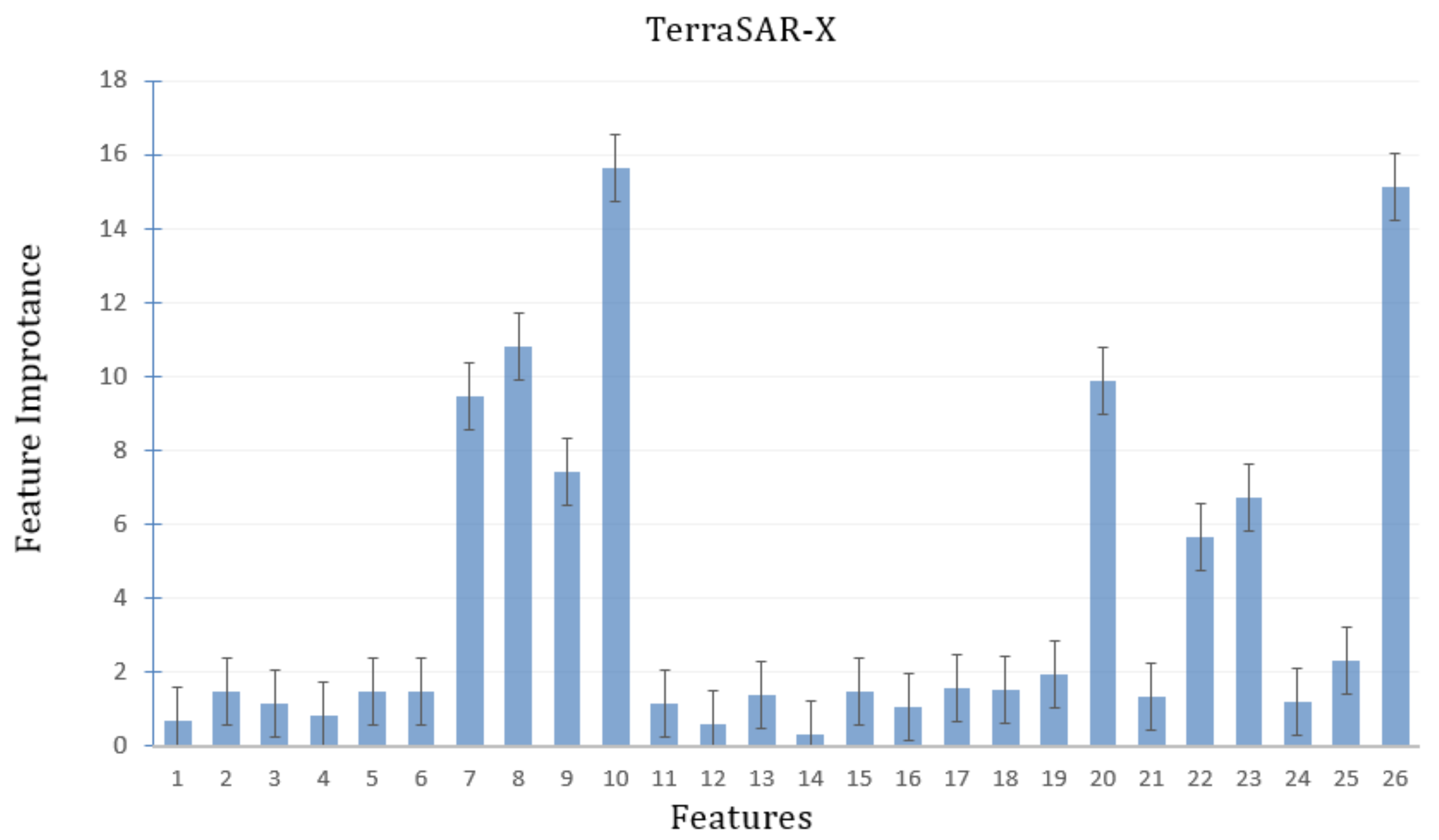
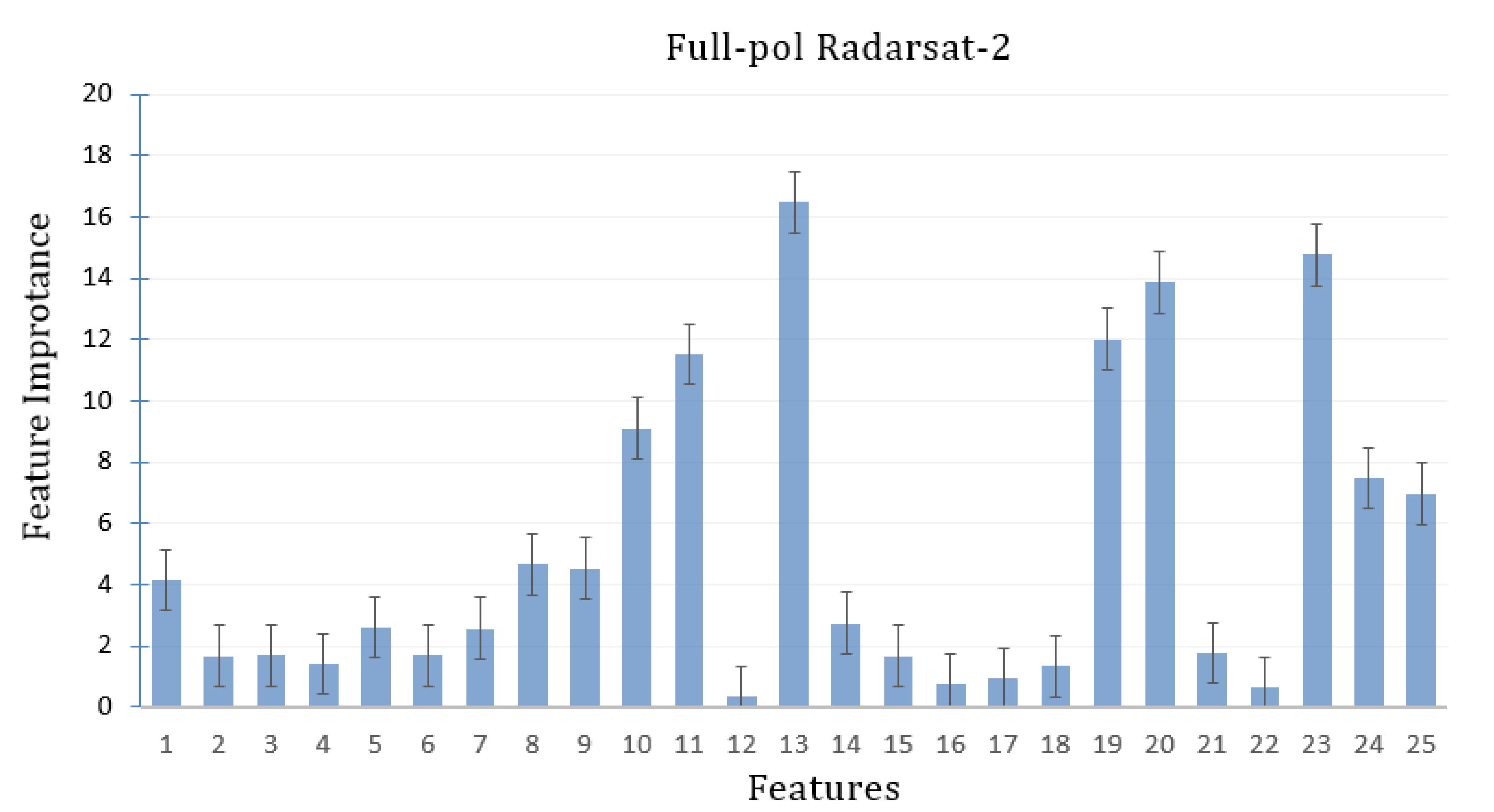
3. Results and Discussion

First, the full-pol data were filtered to eliminate coherent noise. Next, we applied the polarimetric decomposition methods to obtain the polarimetric decomposition components.

Using the different backscattering coefficients and their combinations, as well as different polarimetric components as inputs, we executed a supervised classification. The classification of the polarimetric SAR images was performed using the RF algorithm implemented in R.

Based on the ground data, regions of interest corresponding to winter wheat, PMF, bare soil, urban, and water areas were selected as training areas. A total of 100 samples were collected for each land use type, among them 70% (2520 pixels) and 30% (1080 pixels) were randomly assigned to either training or testing sets, ensuring there was no overlap between the training and testing data.

Using dual-pol SAR data, we carried out both X-band and C-band classification experiments; while both dual-pol and full-pol RADARSAT-2 data were also tested. Classification results obtained for TerraSAR-X, dual-pol RADARSAT-2 and full-pol RADARSAT-2 data are shown in Figure 3, Figure 4 and Figure 5.

To compare the importance of various parameters in this study, we selected the “mean decrease in accuracy” as a measure of importance because it considers the impact of each predictor variable. It is calculated during the out-of-bag error calculation phase of the RF classification and represents the difference between the prediction accuracy before and after permuting the variable of interest. The mean decrease in accuracy is given for each class separately [22,27,33]. The RF algorithm was used to evaluate the importance of these variables, including the backscattering coefficients of different polarizations, their combinations and the different polarimetric decomposition components. Because the importance of these variables may vary with each experimental run, we applied the RF classifier 10 times and used the average values in our analysis.

The importance of TerraSAR-X variables for mapping PMF and other land cover types in Jizhou was ranked as follows: SE_dual, ${\mathsf{\sigma }}_{HH+VV}$, l1, ${\mathsf{\sigma }}_{VV}$, λ, l2, ${\mathsf{\sigma }}_{HH}$, $\left|\langle S_{VV}{S}_{HH}^{*}\rangle \right|$, ${\mathsf{\sigma }}_{HH-VV}$, $\left|{\gamma }_{HHVV}\right|$, α1, α2, p1, A_dual, H1mA, p2, δ1, $\angle \langle S_{VV}{S}_{HH}^{*}\rangle$, ${\mathsf{\sigma }}_{HH/VV}$, 1mHA, H_dual, α, 1mH1mA, HA, δ and δ2. The importance of each of these 26 variables is shown in a bar graph (including their standard deviations) for TerraSAR-X data, as assessed by the RF algorithm (Figure 6).

The importance of dual-pol RADARSAT-2 variables for mapping PMF and other land cover types in Jizhou was ranked as follows: SE_dual, ${\mathsf{\sigma }}_{HH}$, l2, ${\mathsf{\sigma }}_{HH+VV}$, α1, α2, ${\mathsf{\sigma }}_{VV}$, l1, $\left|\langle {\gamma }_{HHVV}\rangle \right|$, ${\mathsf{\sigma }}_{HH-VV}$, λ, α, ${\mathsf{\sigma }}_{HH/VV}$, $\left|\langle S_{VV}{S}_{HH}^{*}\rangle \right|$, H1mA, p1, p2, A_dual, 1mHA, H, HA, 1mH1mA, $\angle \langle S_{VV}{S}_{HH}^{*}\rangle$, δ1, δ and δ2. The importance of each of these 26 variables is shown in a bar graph (including their standard deviations) for dual-pol RADARSAT-2 data, as assessed by the RF algorithm (Figure 7).

The importance of full-pol RADARSAT-2 variables to mapping PMF and other land cover types in Jizhou was ranked as follows: SE_full, ${\mathsf{\sigma }}_{HV}$, F_vol, α, l3, l2, ${\mathsf{\sigma }}_{VV}$, ${\mathsf{\sigma }}_{HH}$, λ, l1, Y_vol, H_full, P₁, P₃, F_odd, P₂, Y_hlx, derd, Y_odd, Y_dbl, A_full, β, δ, F_dbl and γ. The importance of each of these 25 variables is shown in a bar graph (including the standard deviation) for full-pol RADARSAT-2 data, as assessed by the RF algorithm (Figure 8).

Analysis of variable importance (Figure 6, Figure 7 and Figure 8) suggests that the Shannon entropy is the most important variable for classification in all three mapping experiments. Furthermore, the Shannon entropy of the five land cover types was calculated from different SAR data types and compared in Figure 9.

Clearly, the Shannon entropy value of PMF was smaller than that of bare soil in all three data types. Physically, Shannon entropy is a measure of randomness. Both PMF and bare soil are dominated by surface scattering. When PMF is covered, the ground needs to be leveled, and the geometric structure of the ground is changed. After plastic mulching, the randomness of the bare soil declines, making the Shannon entropy value of these two targets different.

It can be seen that Shannon entropy has a similar performance in other studies. Magdalena et al. studied the suitability of the Shannon Entropy for wetland mapping and found that the partially flooded grasslands could be identified and mapped through the Shannon Entropy decomposition [34]. Deng et al. found that three polarimetric features (entropy, Shannon entropy, T11 Coherency Matrix element) and one TF feature (HH intensity of coherence) were most helpful in urban area classification [35]. Chen et al. studied the influence of polarimetric parameters and an object-based approach on land cover classification in coastal wetlands and found that Shannon entropy greatly improved the classification results [36].

The classification accuracy was verified using the confusion matrix method. In this case, the confusion matrix for the classification result corresponding to each method was calculated. The accuracies of the classifications of all five land cover types using different SAR data are provided in

Table 4. The accuracies of the classification of the five land cover types using different SAR data.

SAR Data Type	Mapping Accuracy (%)					User Accuracy (%)					Overall Accuracy (%)	Kappa Coefficient
	PMF	Bare Soil	Wheat	Urban Areas	Water	PMF	Bare Soil	Wheat	Urban Areas	Water
TerraSAR-X	53.28	59.48	93.34	88.27	99.20	64.92	59.82	88.44	85.63	99.38	90.15	0.8464
RADARSAT-2 (HH,VV)	59.56	57.1	91.78	93.79	98.81	56.85	55.98	98.81	92.80	97.82	90.71	0.8545
Full-pol RADARSAT-2	72.56	75.90	98.07	99.93	98.24	70.01	74.51	98.19	96.26	99.86	94.81	0.9189

, including the values for overall accuracy, user accuracy, mapping accuracy and the kappa coefficient, which together describe the classification accuracy from various perspectives.

There are many studies which use decomposition parameters to do land use classification. In the articles using decomposition parameters, there are fewer studies aimed to distinguish between PMF and other ground objects, especially in the comparison of multi-band SAR data.

Our results show that the accuracy of the overall classification of PMF and other land cover types was higher than 90% for all three SAR data types, although the full-pol data had the highest classification accuracy. Both dual-pol TerraSAR-X and RADARSAT-2 data had nearly the same overall accuracy and kappa coefficient values.

Specifically, the classification results based on the TerraSAR-X data show that its mapping accuracies were approximately 53% for PMF, 60% for bare soil, 93% for winter wheat, 88% for urban areas and 99% for water. The kappa coefficient computed for this classification was 0.85. This shows that despite the TerraSAR-X data having a relatively high resolution, they still were not able to distinguish between PMF and bare soil.

The mapping results based on the dual-pol RADARSAT-2 data gave a slightly higher overall accuracy of 90.71%. Its mapping accuracies were approximately 60% for PMF, 57% for bare soil, 92% for winter wheat, 94% for urban areas and 99% for water. These data also could not discriminate effectively between PMF and bare soil. Their kappa coefficient was 0.86.

In contrast, the mapping results based on the full-pol RADARSAT-2 data gave an overall accuracy of 95%. Mapping accuracies based on these data were approximately 73% for PMF, 76% for bare soil, 94% for winter wheat, 98% for urban areas and 99.9% for water. The kappa coefficient for this classification was 0.92, which indicates that it was very good. In Table 4, misclassification of pixels mainly occurred because of confusion between PMF and bare soil. Such misclassification reflected the similar responses of these land covers to SAR signals.

4. Conclusions

The development of polarization decomposition technology has allowed polarization decomposition to be more widely used for remote sensing image classification. However, few studies have systematically compared classifications based on different SAR bands, especially when applied to the remote sensing classification of PMF.

In this study, we evaluated the classification of PMF and other land cover types using the features obtained from the decomposition components of three SAR data types (i.e., TerraSAR-X, dual-pol RADARSAT-2 and full pol RADARSAT-2) for a study area in Jizhou, China. Overall, in this study the accuracy of classification using the full-pol SAR data was higher than both dual-pol data types. We showed that the classification accuracy of PMF using the full-pol RADARSAT-2 SAR data was higher than 70%. Analysis of the importance of polarization parameters showed that the Shannon entropy made the greatest contribution to mapping accuracy.

References

1. Bai, L.; Hai, J.; Han, Q.; Jia, Z. Effects of mulching with different kinds of plastic film on growth and water use efficiency of winter wheat in Weibei Highland. Agric. Res. Arid Areas 2010, 28, 135–139. [Google Scholar]
2. Yan, C.; Mei, X.; He, W.; Zheng, S. Present situation of residue pollution of mulching plastic film and controlling measures. Trans. Chin. Soc. Agric. Eng. 2006, 22, 269–272. [Google Scholar]
3. Lu, L.; Di, L.; Ye, Y. A Decision-Tree Classifier for Extracting Transparent Plastic-Mulched Landcover from Landsat-5 TM Images. IEEE J.-STARS 2014, 7, 4548–4558. [Google Scholar] [CrossRef]
4. Picuno, P.; Tortora, A.; Capobianco, R.L. Analysis of plasticulture landscapes in southern Italythrough remote sensing and solid modeling techniques. Landsc. Urban Plan. 2011, 100, 45–56. [Google Scholar] [CrossRef]
5. Levin, N.; Lugassi, R.; Ramon, U.; Braun, O.; Ben-Dor, E. Remote sensing as a tool formonitoring plasticulture in agricultural landscapes. Int. J. Remote Sens. 2007, 28, 183–202. [Google Scholar] [CrossRef]
6. Lanorte, A.; De Santis, F.; Nolè, G.; Blanco, I.; Loisi, R.V.; Schettini, E.; Vox, G. Agricultural plastic waste spatial estimation by landsat 8 satellite images. Comput. Electron. Agric. 2017, 141, 35–45. [Google Scholar] [CrossRef]
7. Novelli, A.; Aguilar, M.A.; Nemmaoui, A.; Aguilar, F.J.; Tarantino, E. Performance evaluation of object based greenhouse detection from sentinel-2 msi and landsat 8 oli data: A case study from almería (Spain). Int. J. Appl. Earth Obs. Geoinf. 2016, 52, 403–411. [Google Scholar] [CrossRef]
8. Carvajal, F.; Crisanto, E.; Aguilar, F.J.; Aguera, F.; Aguilar, M.A. Green-houses detection using an artificial neural network with a very high resolution satellite image. In Proceedings of the ISPRS Technical Commission II Symposium, Vienna, Austria, 12–14 July 2006; pp. 37–42. [Google Scholar]
9. Agüera, F.; Liu, J.G. Automatic greenhouse delineation from quickbird and ikonos satellite images. Comput. Electron. Agric. 2009, 66, 191–200. [Google Scholar] [CrossRef]
10. Hasituya; Chen, Z.; Wang, L.; Wu, W.; He, L. Monitoring plastic-mulched farmland by landsat-8 oli imagery using spectral and textural features. Remote Sens. 2016, 8, 353. [Google Scholar] [CrossRef]
11. Yang, D.; Jin, C.; Yuan, Z.; Xiang, C.; Chen, X.; Xin, C. Mapping plastic greenhouse with medium spatial resolution satellite data: Development of a new spectral index. Isprs J. Photogramm. Remote Sens. 2017, 128, 47–60. [Google Scholar] [CrossRef]
12. Mcnairn, H.; Shang, J.; Champagne, C.; Jiao, X. Terrasar-x and RADARSAT-2 for crop classification and acreage estimation. In Proceedings of the 2009 IEEE International Geoscience and Remote Sensing Symposium, Cape Town, South Africa, 12–17 July 2009. [Google Scholar]
13. Qin, M.; Wang, J.; Shang, J.; Peng, W. Assessment of multi-temporal RADARSAT-2 polarimetric sar data for crop classification in an urban/rural fringe area. In Proceedings of the 2013 Second International Conference on Agro-Geoinformatics (Agro-Geoinformatics), Fairfax, VA, USA, 12–16 August 2013. [Google Scholar]
14. Skakun, S.; Kussul, N.; Shelestov, A.Y.; Lavreniuk, M.; Kussul, O. Efficiency assessment of multitemporal c-band RADARSAT-2 intensity and landsat-8 surface reflectance satellite imagery for crop classification in ukraine. IEEE J. Sel. Top. Appl. Earth Obs. Remote Sens. 2016, 9, 3712–3719. [Google Scholar] [CrossRef]
15. Jiao, X.; Kovacs, J.M.; Shang, J.; Mcnairn, H.; Dan, W.; Ma, B.; Geng, X. Object-oriented crop mapping and monitoring using multi-temporal polarimetric RADARSAT-2 data. Isprs J. Photogramm. Remote Sens. 2014, 96, 38–46. [Google Scholar] [CrossRef]
16. Sonobe, R.; Tani, H.; Wang, X.; Kobayashi, N.; Shimamura, H. Random forest classification of crop type using multi-temporal terrasar-x dual-polarimetric data. Remote Sens. Lett. 2014, 5, 157–164. [Google Scholar] [CrossRef]
17. Li, Y.; Lampropoulos, G. RADARSAT-2 and terrasar-x polarimetric data for crop growth stages estimation. In Proceedings of the 2016 IEEE International Geoscience and Remote Sensing Symposium (IGARSS), Beijing, China, 10–15 July 2016. [Google Scholar]
18. Hasituya; Chen, Z.; Li, F.; Hong, M. Mapping Plastic-Mulched Farmland with C-Band Full Polarization SAR Remote Sensing Data. Remote Sens. 2017, 9, 1264. [Google Scholar] [CrossRef]
19. Lu, L.; Tao, Y.; Di, L. Object-based plastic-mulched landcover extraction using integrated Sentinel-1 and Sentinel-2 data. Remote Sens. 2018, 10, 1820. [Google Scholar] [CrossRef]
20. Cloude, S.; Pottier, E. An entropy based classification scheme for land applications of polarimetric SAR. IEEE Trans. Geosci. Remote Sens. 1997, 35, 68–78. [Google Scholar] [CrossRef]
21. Cloude, S. The Dual Polarization Entropy/Alpha Decomposition: A PALSAR Case Study. In Proceedings of the 3rd International Workshop on Science and Applications of SAR Polarimetry and Polarimetric Interferometry, Frascati, Italy, 22–26 January 2007; pp. 1–6. [Google Scholar]
22. Heine, I.; Jagdhuber, T.; Itzerott, S. Classification and monitoring of reed belts using dual-polarimetric terrasar-x time series. Remote Sens. 2016, 8, 552. [Google Scholar] [CrossRef]
23. Morio, J.; Refregier, P.; Goudail, F.; Dubois-Fernandez, P.C.; Dupuis, X. Information theory-based approach for contrast analysis in polarimetric and/or interferometric sar images. IEEE Trans. Geosci. Remote Sens. 2008, 46, 2185–2196. [Google Scholar] [CrossRef]
24. Philippe, R.; Jérôme, M. Entropy-Shannon of partially polarized and partially coherent light with gaussian fluctuations. J. Opt. Soc. Am. A Opt. Image Sci. Vis. 2006, 23, 3036–3044. [Google Scholar]
25. Freeman, A.; Durden, S.L. A three-component scattering model for polarimetric sar data. IEEE Trans. Geosci. Remote Sens. 1998, 36, 963–973. [Google Scholar] [CrossRef]
26. Yamaguchi, Y.; Moriyama, T.; Ishido, M.; Yamada, H. Four-component scattering model for polarimetric sar image decomposition. Tech. Rep. Ieice Sane 2005, 104, 1699–1706. [Google Scholar] [CrossRef]
27. Breiman, L. Random forests. Mach. Learn. 2001, 45, 5–32. [Google Scholar] [CrossRef]
28. Gislason, P.O.; Benediktsson, J.A.; Sveinsson, J.R. Random Forests for land cover classification. Pattern Recognit. Lett. 2006, 27, 294–300. [Google Scholar] [CrossRef]
29. Rodriguez-Galiano, V.F.; Chica-Olmo, M.; Abarca-Hernandez, F.; Atkinson, P.M.; Jeganathan, C. Random Forest classification of Mediterranean land cover using multi-seasonal imagery and multi-seasonal texture. Remote Sens. Environ. 2012, 121, 93–107. [Google Scholar] [CrossRef]
30. Dabboor, M.; Montpetit, B.; Howell, S. Assessment of the high resolution sar mode of the radarsat constellation mission for first year ice and multiyear ice characterization. Remote Sens. 2018, 10, 594. [Google Scholar] [CrossRef]
31. Tong, S.; Liu, X.; Chen, Q.; Zhang, Z.; Xie, G. Multi-feature based ocean oil spill detection for polarimetric sar data using random forest and the self-similarity parameter. Remote Sens. 2019, 11, 451. [Google Scholar] [CrossRef]
32. Chen, W.; Li, X.; He, H.; Wang, L. Assessing different feature sets’ effects on land cover classification in complex surface-mined landscapes by ziyuan-3 satellite imagery. Remote Sens. 2017, 10, 23. [Google Scholar] [CrossRef]
33. Loosvelt, L.; Peters, J.; Skriver, H.; Baets, B.D.; Verhoest, N.E.C. Impact of reducing polarimetric sar input on the uncertainty of crop classifications based on the random forests algorithm. IEEE Trans. Geosci. Remote Sens. 2012, 50, 4185–4200. [Google Scholar] [CrossRef]
34. Mleczko, M.; Mróz, M. Wetland mapping using sar data from the sentinel-1a and tandem-x missions: A comparative study in the biebrza floodplain (poland). Remote Sens. 2018, 10, 78. [Google Scholar] [CrossRef]
35. Lei, D.; Yan, Y.N.; Wang, C. Improved polsar image classification by the use of multi-feature combination. Remote Sens. 2015, 7, 4157–4177. [Google Scholar]
36. Chen, Y.; He, X.; Jing, W.; Xiao, R. The influence of polarimetric parameters and an object-based approach on land cover classification in coastal wetlands. Remote Sens. 2014, 6, 12575–12592. [Google Scholar] [CrossRef]
Figure 1. The location of the study area and the distribution of samples. Detail is shown on a GF-1 satellite image of the study area. The five land cover classes sampled were: plastic-mulched farmland (cyan dots), buildings (red dots), bare soil (yellow dots), winter wheat (green dots) and water (blue dots).
Remotesensing 11 00660 g001
Figure 2. Flowchart for polarimetric SAR data processing.
Remotesensing 11 00660 g002
Figure 3. Classification map based on dual-polarimetric TerraSAR-X data.
Remotesensing 11 00660 g003
Figure 4. Classification map based on dual-polarimetric RADARSAT-2 data.
Remotesensing 11 00660 g004
Figure 5. Classification map based on full-polarimetric RADARSAT-2 data.
Remotesensing 11 00660 g005
Figure 6. Bar graph of the average and standard deviation values of the importance of each variable to mapping of plastic-mulched farmland and other land cover types in Jizhou using dual-polarimetric TerraSAR-X data, as assessed by the random forest algorithm. Values 1–26 reflect their listing in Table 2.
Remotesensing 11 00660 g006
Figure 7. Bar graph of the average and standard deviation values of the importance of each variable to mapping of plastic-mulched farmland and other land cover types in Jizhou using dual-polarimetric RADARSAT-2 data, as assessed by the random forest algorithm. Values 1–26 reflect their listing in Table 2.
Remotesensing 11 00660 g007
Figure 8. Bar graph of the average and standard deviation values of the importance of each variable to mapping of plastic-mulched farmland and other land cover types in Jizhou using full-polarimetric RADARSAT-2 data, as assessed by the random forest algorithm. Values 1–25 reflect their listing in Table 3.
Remotesensing 11 00660 g008
Figure 9. Shannon entropy of all five land cover types calculated from different synthetic aperture radar data (i.e., full-polarimetric RADARSAT-2, dual-polarimetric RADARSAT-2 and dual-polarimetric TerraSAR-X).
Remotesensing 11 00660 g009