Author Contributions
Conceptualization, L.L.; Funding acquisition, J.X.; Project administration, J.X.; Supervision, J.X. and Y.W.; Validation, L.L., J.X. and Y.W.; Visualization, L.L.; Writing—original draft, L.L.; Writing—review & editing, J.X. and Y.W.
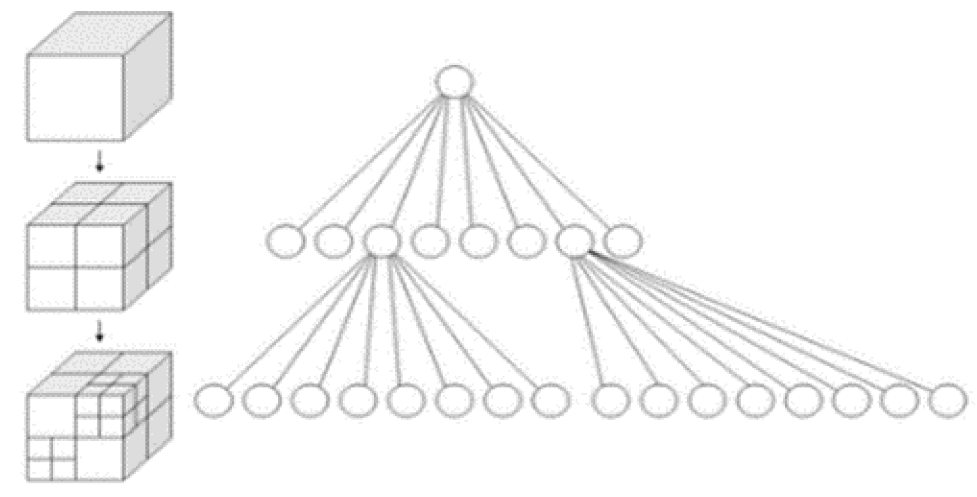
Figure 1.
Spatial grid structure
Figure 1.
Spatial grid structure
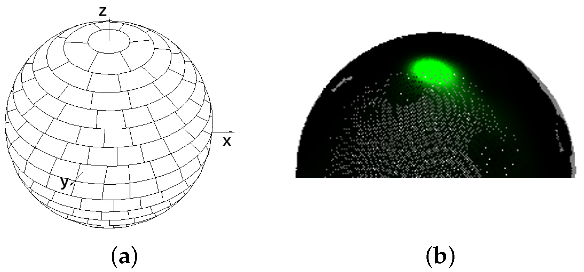
Figure 2.
The accumulator design. (a) Accumulator ball. (b) Result of voting.
Figure 2.
The accumulator design. (a) Accumulator ball. (b) Result of voting.
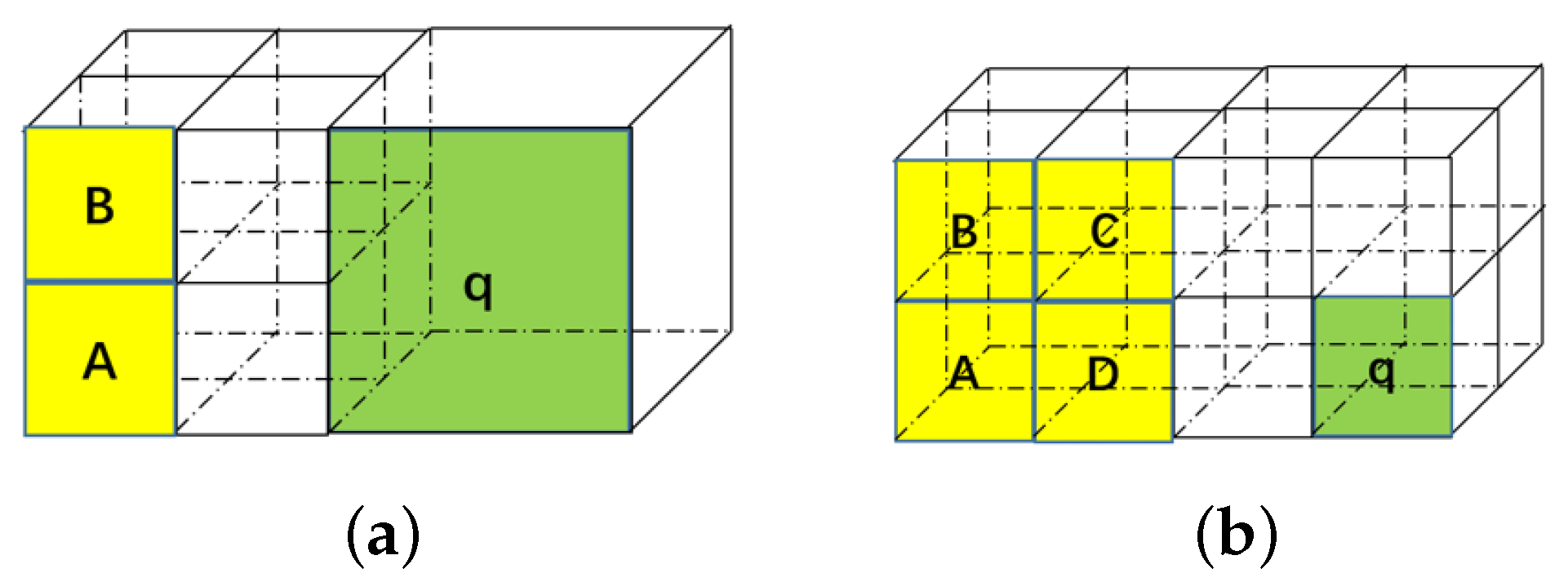
Figure 3.
The neighbor voxels of q, (a) q is a big-voxel, A and B are sub-voxels. The relationship between A (or B) and q is coplanar but not adjacent; (b) None of is the neighbor voxel of q.
Figure 3.
The neighbor voxels of q, (a) q is a big-voxel, A and B are sub-voxels. The relationship between A (or B) and q is coplanar but not adjacent; (b) None of is the neighbor voxel of q.
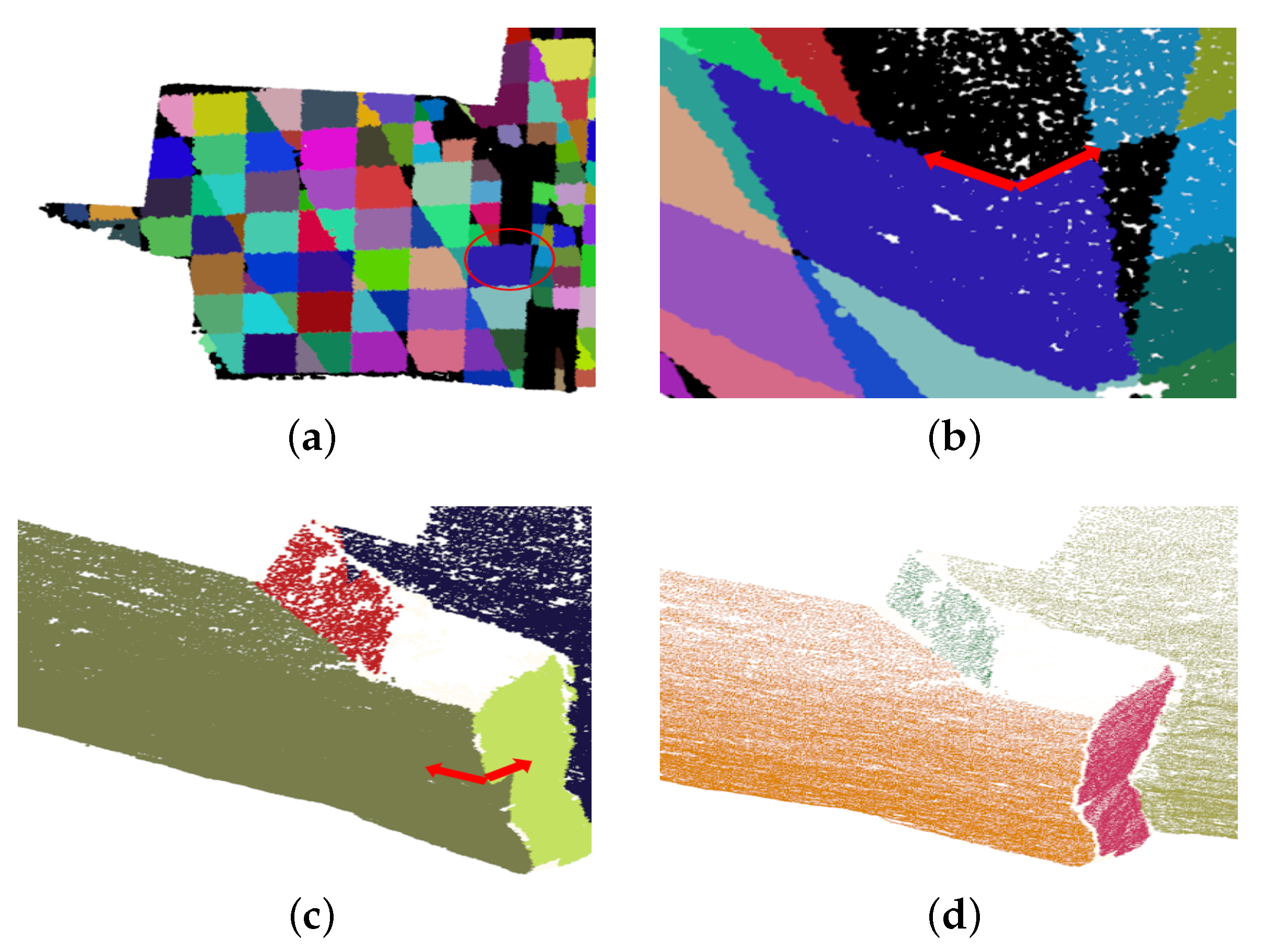
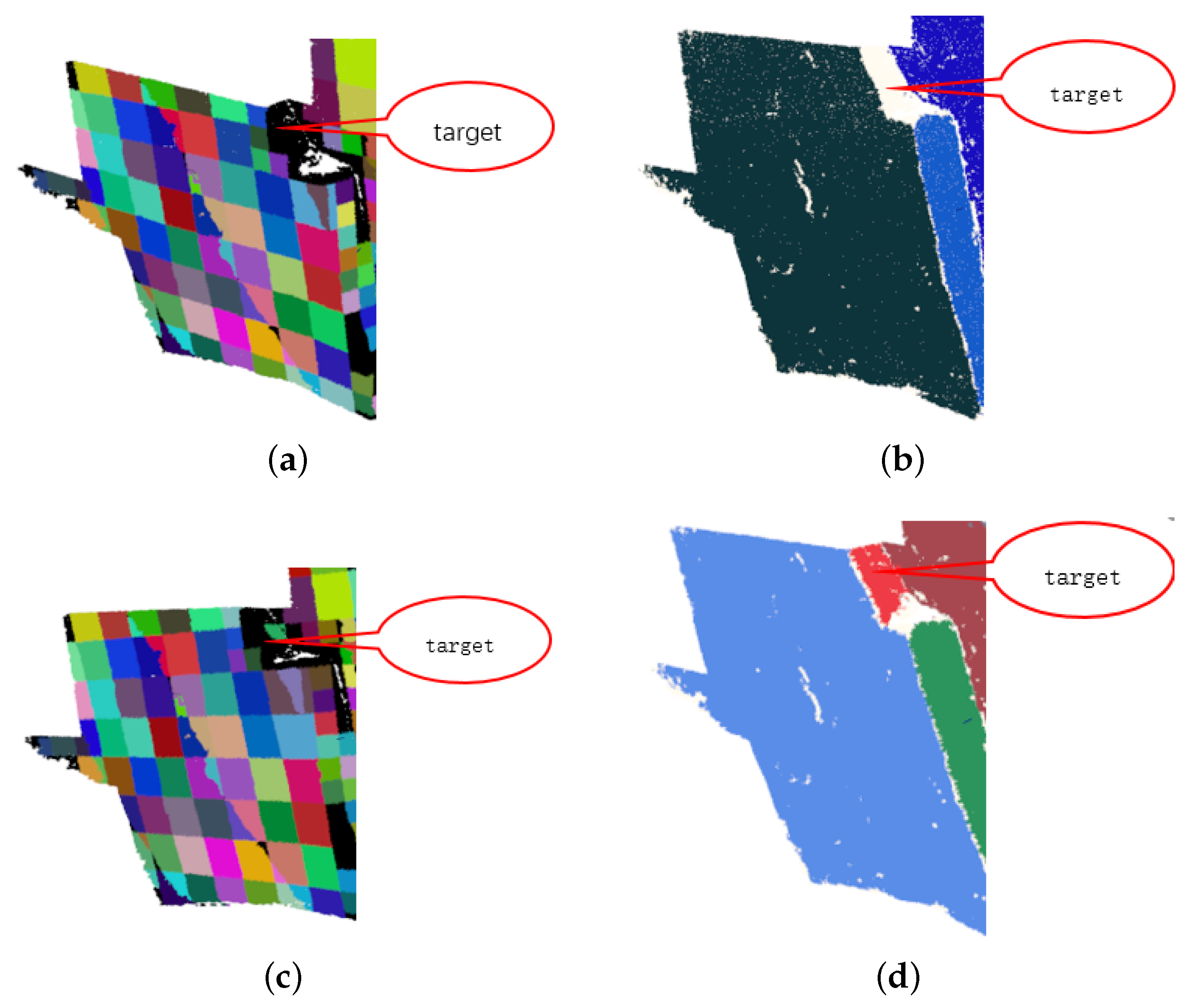
Figure 4.
The coplanar voxels may be not “really coplanar”. (a) The result of clustering; (b) The partial enlarged view of (a); (c) The finally result of surface extraction without considering the non-coplanar points in coplanar voxels; (d) The finally result of surface extraction with Algorithm 5.
Figure 4.
The coplanar voxels may be not “really coplanar”. (a) The result of clustering; (b) The partial enlarged view of (a); (c) The finally result of surface extraction without considering the non-coplanar points in coplanar voxels; (d) The finally result of surface extraction with Algorithm 5.
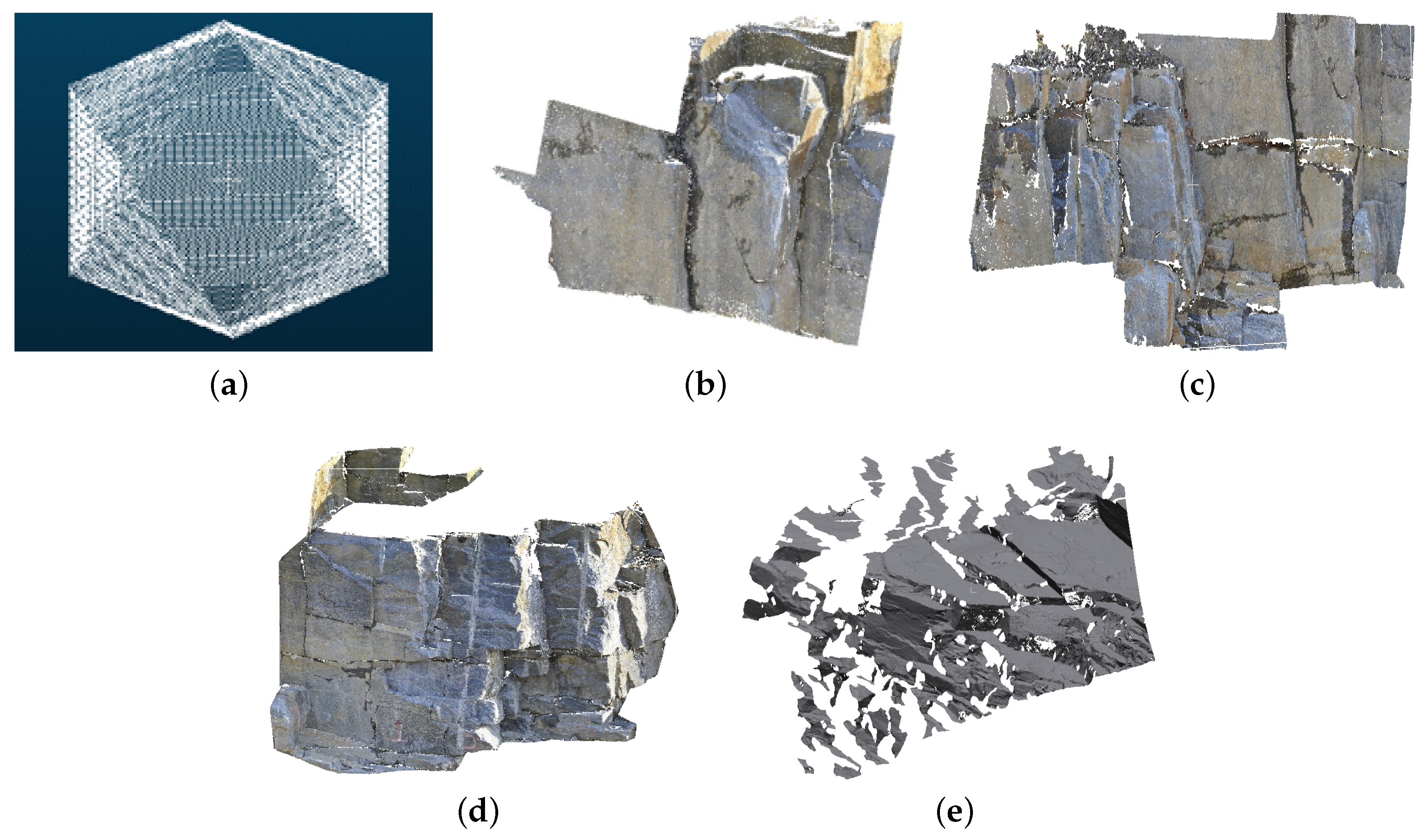
Figure 5.
The display of 5 point clouds. (a) Icosahedron; (b) Rock1; (c) Rock2; (d) Rock3 and (e) Rock4.
Figure 5.
The display of 5 point clouds. (a) Icosahedron; (b) Rock1; (c) Rock2; (d) Rock3 and (e) Rock4.
Figure 6.
The results of clustering and rock surface extraction with different parameters. (a,b) Results of clustering and rock surface extraction respectively (). (c,d) Results of clustering and rock surface extraction respectively ().
Figure 6.
The results of clustering and rock surface extraction with different parameters. (a,b) Results of clustering and rock surface extraction respectively (). (c,d) Results of clustering and rock surface extraction respectively ().
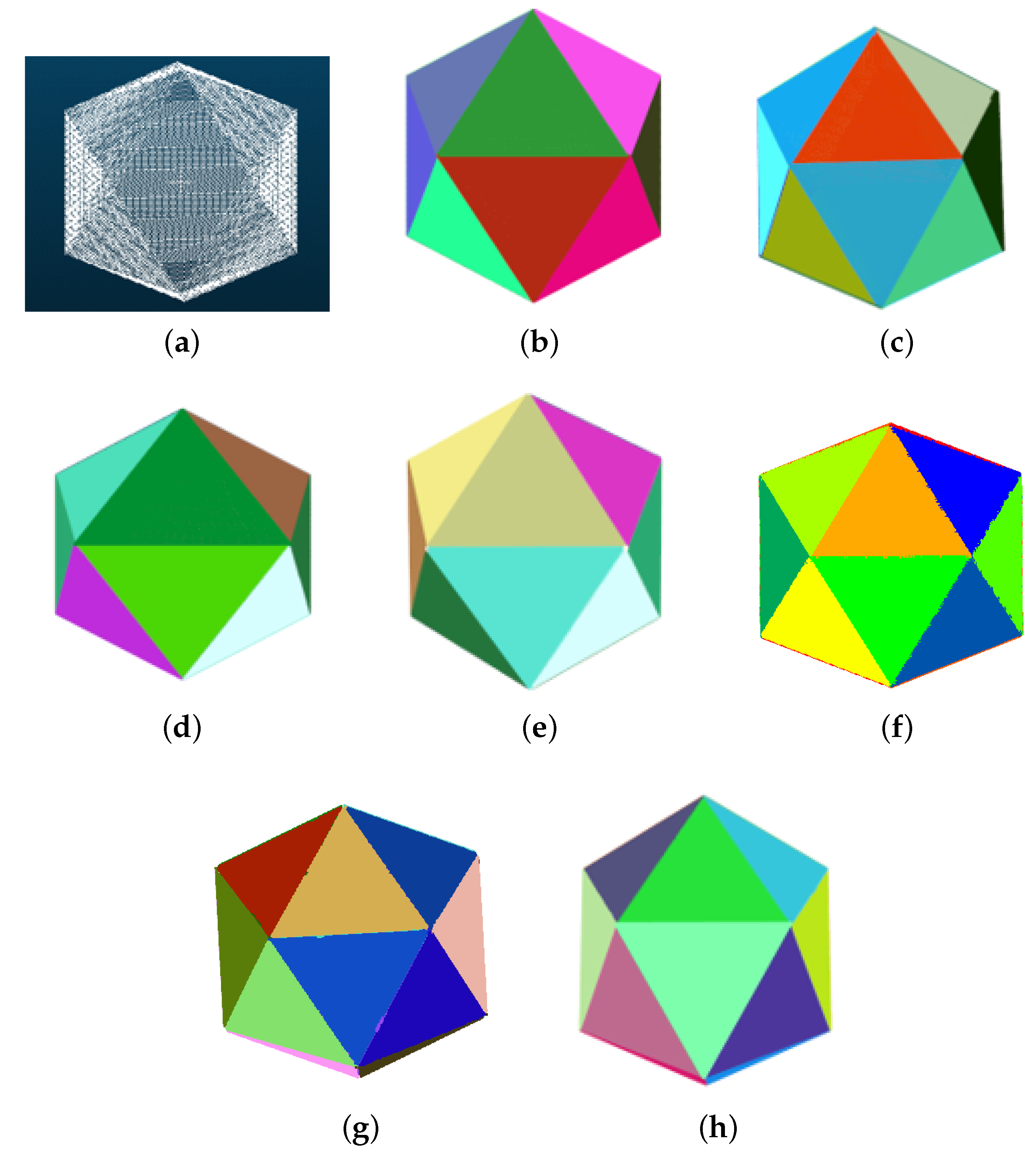
Figure 7.
The feature surface extraction results of 7 methods for icosahedron. (a) Original icosahedron point cloud; (b–h) Results of RHT, RG, RAN_PCL, RAN_CGAL, DSE, HT-RG and our method respectively.
Figure 7.
The feature surface extraction results of 7 methods for icosahedron. (a) Original icosahedron point cloud; (b–h) Results of RHT, RG, RAN_PCL, RAN_CGAL, DSE, HT-RG and our method respectively.
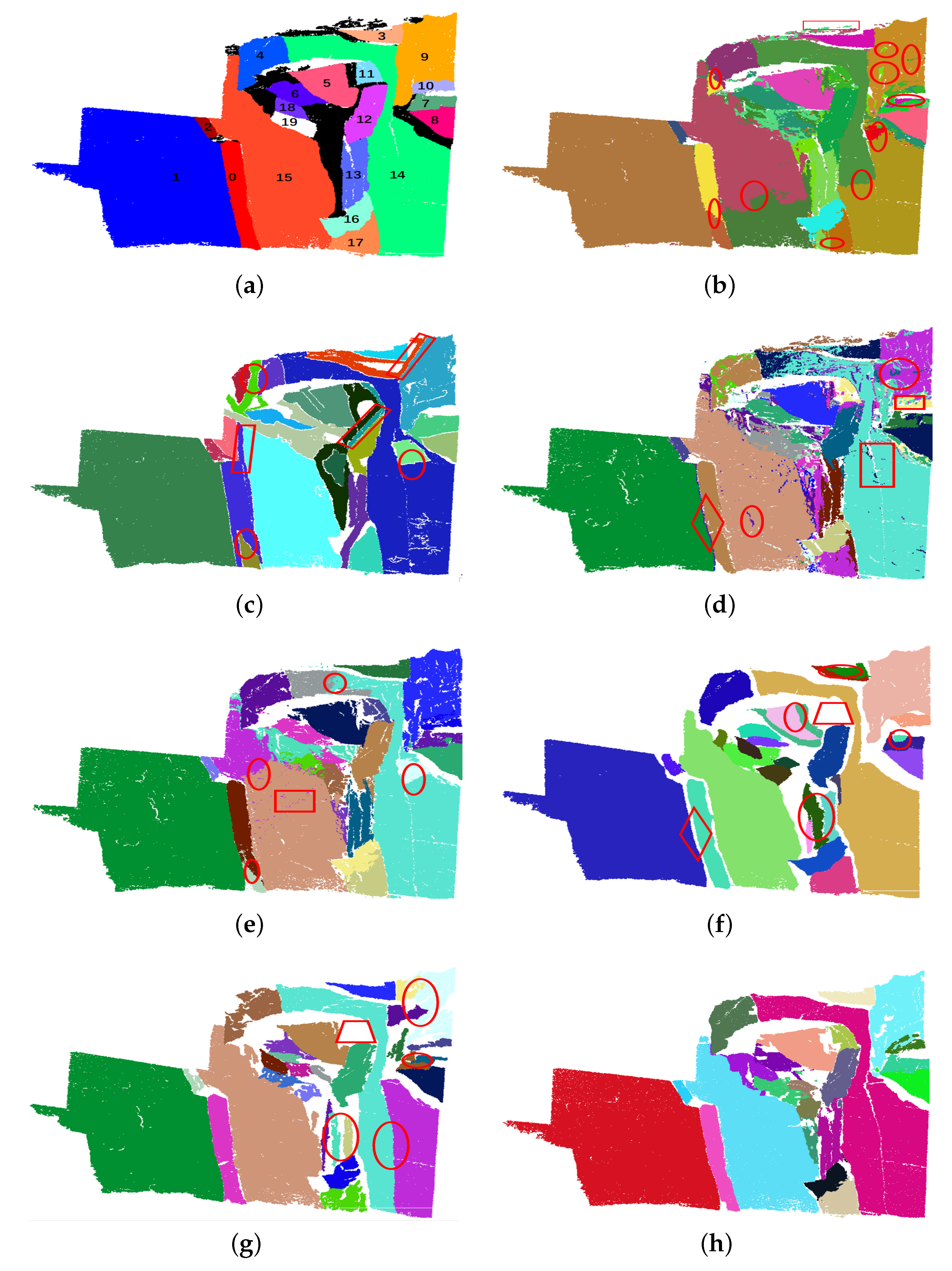
Figure 8.
The rock surface extraction results of seven different methods for Rock1. (a) The reference point cloud of Rock1. (b–h) Results of RHT, RG, RAN_PCL, RAN_CGAL, HT_RG, DSE and ours, respectively. Each color represents a surface. Notice that, we use red polygons to point out the deficiencies of each result. Ellipse indicates over-segmentation, rectangle represents discontinuity, parallelogram represents incorrect result, rhombus represent bad boundary and trapezoid represents missing detection.
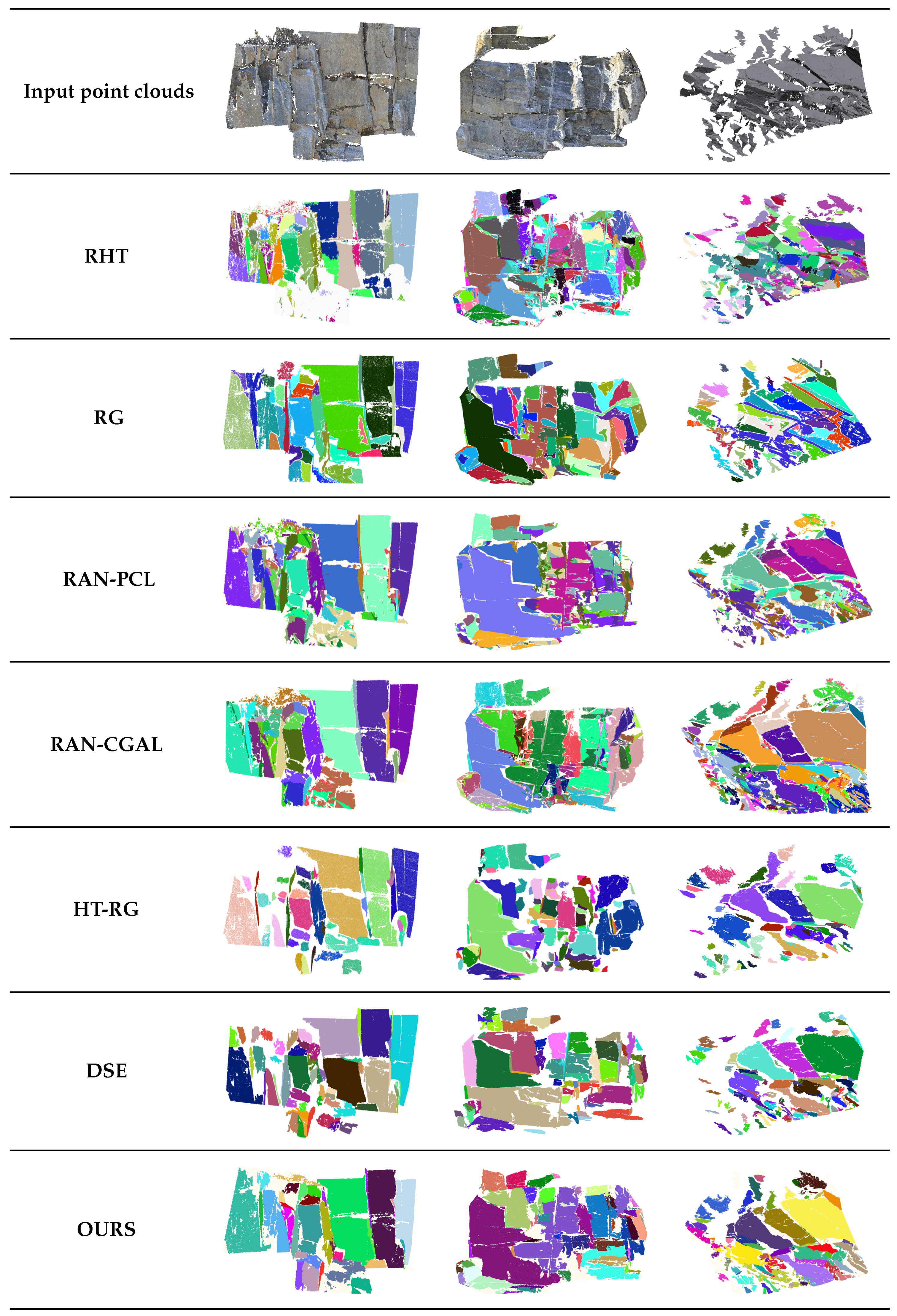
Figure 9.
The results of different methods for three other Rock-Mass point clouds.
Figure 9.
The results of different methods for three other Rock-Mass point clouds.
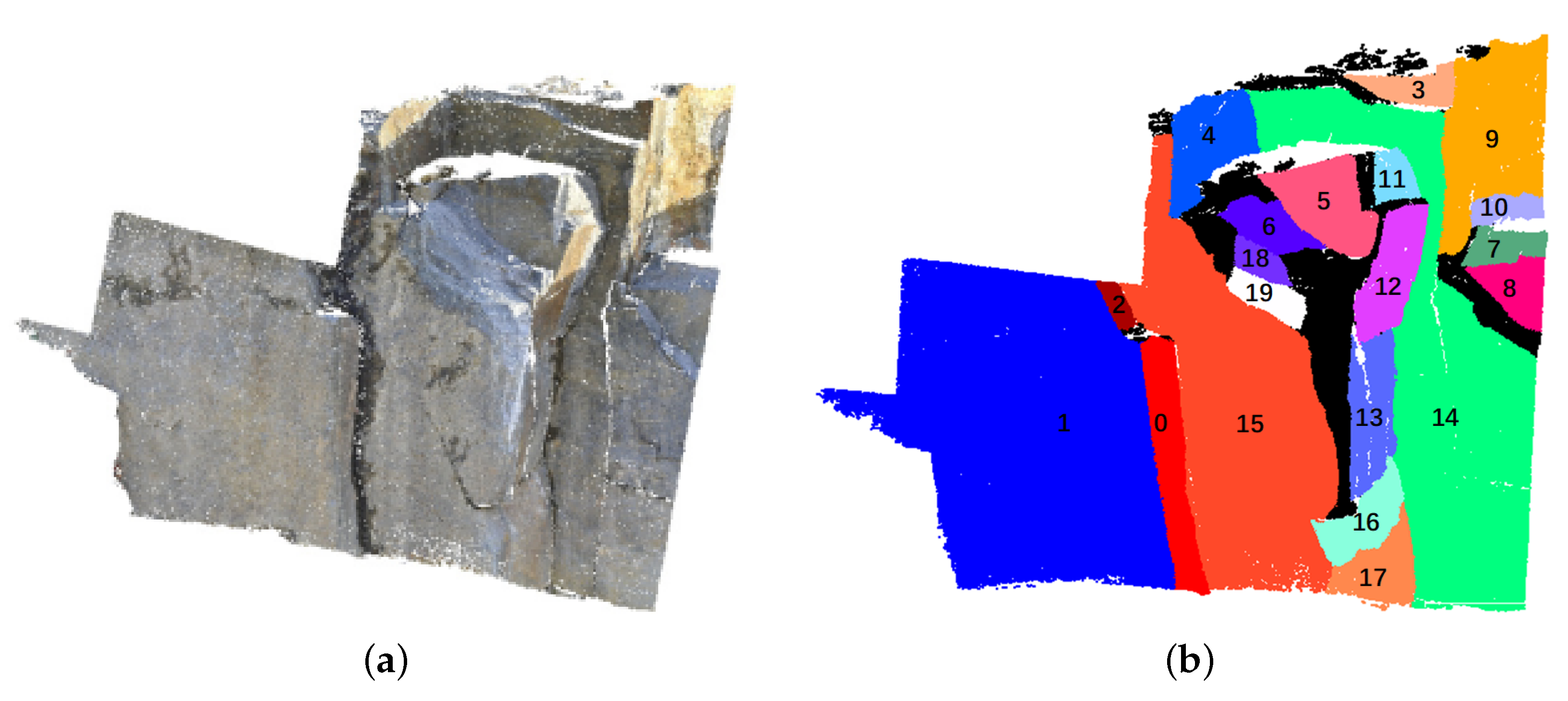
Figure 10.
The reference point cloud of rock mass. (a) The original point cloud of Rock1. (b) The reference point cloud of Rock1. In addition to black, each of the other colors represents a separated surface.
Figure 10.
The reference point cloud of rock mass. (a) The original point cloud of Rock1. (b) The reference point cloud of Rock1. In addition to black, each of the other colors represents a separated surface.
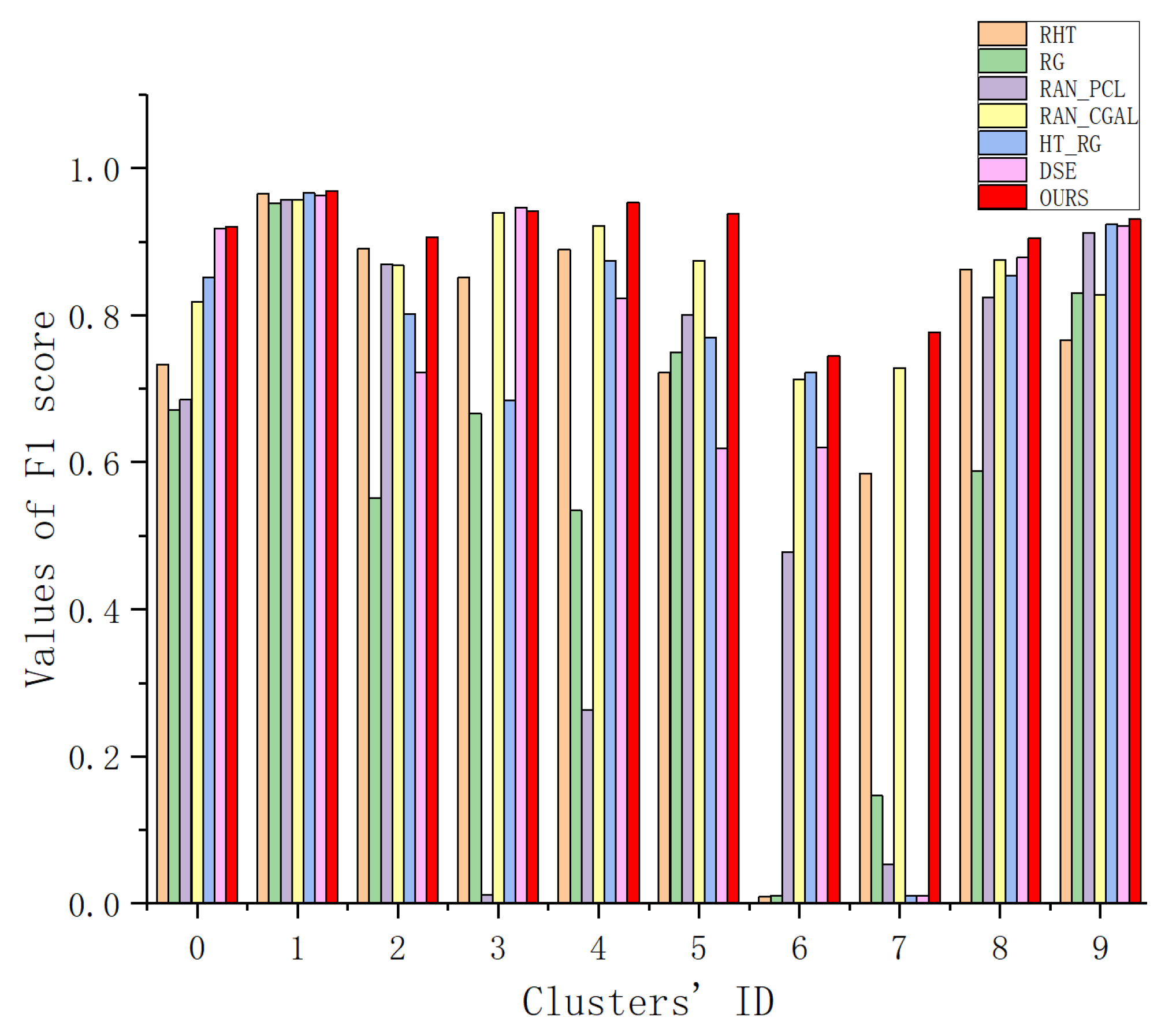
Figure 11.
F1 scores of Rock1’s feature surfaces for different methods.
Figure 11.
F1 scores of Rock1’s feature surfaces for different methods.
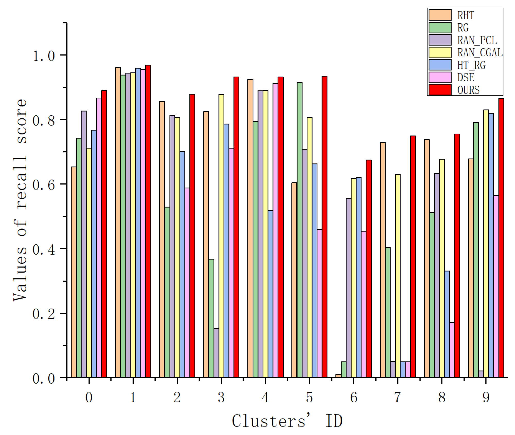
Figure 12.
Recall scores of Rock1’s feature surfaces for different methods.
Figure 12.
Recall scores of Rock1’s feature surfaces for different methods.
Table 1.
The information of 5 point clouds.
Table 1.
The information of 5 point clouds.
| Name | Number of Points | Maximum Point Spacing (m) | Minimum Point Spacing (m) | Average Point Spacing (m) | Bounding Box Size (m) |
|---|
| Icosahedron | 372,140 | 0.1308 | | 0.0634 | |
| Rock1 | 387,610 | 0.5167 | 0.0299 | 0.0396 | |
| Rock2 | 264,309 | 0.4663 | 0.0499 | 0.0639 | |
| Rock3 | 1,178,578 | 0.8016 | 0.0244 | 0.0311 | |
| Rock4 | 1,024,521 | 0.1728 | 0.0009 | 0.0191 | |
Table 2.
Summary of the parameters.
Table 2.
Summary of the parameters.
| Stage | ID | Parameters | Meaning | Configuration method |
|---|
| Clustering | 1 | knn | Neighbors for estimating the normal | Related to the spatial extent of feature surfaces. Set manually. |
| 2 | | The length of big voxel | Related to the spatial extend of feature surfaces. Set manually. |
| 3 | | Allowable maximum ratio about and | 20–40, related to the roughness of the surface. Set manually. |
| 4 | | Allowable maximum MSE value of coplanar voxels | 0.05–0.15, related to the roughness of the surface. Set manually. |
| 5 | | Minimum number of points in a big voxel | Related to the sample densities of the point cloud and . Set manually. |
| 6 | | Minimum number of points in a small voxel | Related to the sample densities of the point cloud and . Set manually. |
| Major orientation estimation | 1 | | The discretization of | Default is 180. |
| 2 | | The discretization of | Default is 360. |
| 3 | | The weight coefficient of the edge length of voxel | Default is 0.75. |
| 4 | | The weight coefficient of the points contained in voxel | Default is 0.25 . |
| 5 | | The size of sliding-window | Default is 8. |
| Rock surface extraction | 1 | | Allowable maximum distance between a point to a surface or a surface to another surface | Related to the roughness of the surface. Set manually. |
| 2 | | Allowable minimum number of points in a surface | Related to the spatial extent of feature surfaces. Set manually. |
| 3 | | Maximum angle between major orientation and the normal vector of voxel | |
| 4 | | Maximum angle between the normal vector of surface and the normal vector of neighbor voxel | |
| 5 | | Maximum angle between the normal vector of point and the normal vector of surface | . Default is |
Table 3.
The parameter setting of our method.
Table 3.
The parameter setting of our method.
| Parameter | Icosahedron | Rock1 | Rock2 | Rock3 | Rock4 |
|---|
| knn | 50 | 80 | 80 | 80 | 80 |
| 6 | 1.73 | 1.73 | 1.70 | 1.50 |
| 40 | 30 | 22.5 | 30 | 30 |
| 0.05 | 0.05 | 0.05 | 0.05 | 0.05 |
| 150 | 150 | 150 | 300 | 300 |
| 300 | 300 | 300 | 600 | 600 |
| 0.1 | 0.3 | 0.3 | 0.3 | 0.3 |
| 2000 | 900 | 900 | 1000 | 1000 |
| | | | | |
| | | | | |
Table 4.
Execution time of 7 different methods for icosahedron (in seconds).
Table 4.
Execution time of 7 different methods for icosahedron (in seconds).
| Method | Time (s) | Number of Detected Surfaces |
|---|
| RHT | 2.083 | 20 |
| RG | 7.678 | 20 |
| RAN_PCL | 19.068 | 20 |
| RAN_CGAL | 1.802 | 20 |
| DSE | 90.810 | 20 |
| HT-RG | 8.780 | 20 |
| Ours | 0.246 | 20 |
Table 5.
Execution time of 7 different methods for Rock1 (in seconds).
Table 5.
Execution time of 7 different methods for Rock1 (in seconds).
| Method | Time (s) | Number of Detected Surfaces |
|---|
| RHT | 7.312 | 25 |
| RG | 15.122 | 25 |
| RAN_PCL | 22.342 | 25 |
| RAN_CGAL | 2.869 | 26 |
| HT_RG | 59.606 | 29 |
| DSE | 108.684 | 30 |
| Ours | 0.445 | 23 |
Table 6.
Time distribution of our method (in seconds).
Table 6.
Time distribution of our method (in seconds).
| Date | Number of Points | Clustering | Major Orientation Estimation | Region Growing | Total |
|---|
| Icosahedron | 372,140 | 0.03644 | 0.08542 | 0.12414 | 0.24600 |
| Rock1 | 387,610 | 0.05572 | 0.12329 | 0.26621 | 0.44522 |
| Rock2 | 264,309 | 0.06060 | 0.12159 | 0.24291 | 0.42510 |
| Rock3 | 1,178,578 | 0.11082 | 0.18914 | 1.36345 | 1.66341 |
| Rock4 | 1,024,521 | 0.07757 | 0.13365 | 0.51241 | 0.72363 |
Table 7.
Rock1’s accuracy.
Table 7.
Rock1’s accuracy.
| Method | Precision | Recall | F1 |
|---|
| RHT | 74.23% | 77.53% | 75.85% |
| RG | 77.98% | 76.23% | 77.10% |
| RAN-PCL | 81.70% | 81.17% | 81.43% |
| RAN-CGAL | 85.42% | 83.66% | 84.53% |
| HT-RG | 91.18% | 86.37% | 88.71% |
| DSE | 81.28% | 74.77% | 77.89% |
| OURS | 91.92% | 91.67% | 91.80% |


