Fusion of Multispectral and Panchromatic Images via Spatial Weighted Neighbor Embedding

Abstract

Fusing the panchromatic (PAN) image and low spatial-resolution multispectral (LR MS) images is an effective technology for generating high spatial-resolution MS (HR MS) images. Some image-fusion methods inspired by neighbor embedding (NE) are proposed and produce competitive results. These methods generally adopt Euclidean distance to determinate the neighbors. However, closer Euclidean distance is not equal to greater similarity in spatial structure. In this paper, we propose a spatial weighted neighbor embedding (SWNE) approach for PAN and MS image fusion, by exploring the similar manifold structures existing in the observed LR MS images to those of HR MS images. In SWNE, the spatial neighbors of the LR patch are found first. Second, the weights of these neighbors are estimated by the alternative direction multiplier method (ADMM), in which the neighbors and their weights are determined simultaneously. Finally, the HR patches are reconstructed by the sum of HR patches corresponding to the LR patches multiplying with their weights. Due to the introduction of spatial structures in objective function, outlier patches can be eliminated effectively by ADMM. Compared with other methods based on NE, more reasonable neighbor patches and their weights are estimated simultaneously. Some experiments are conducted on datasets collected by QuickBird and Geoeye-1 satellites to validate the effectiveness of SWNE, and the results demonstrate a better performance of SWNE in spatial and spectral information preservation.

1. Introduction

With the progressive development of remote-sensing technology, many satellites are launched to provide both urban and rural observation for target recognition [1] and classification [2]. Due to physical limitations of sensors, it is difficult to achieve high resolution in both the spatial and spectral domain. However, the high spatial-resolution panchromatic (PAN) image and the low spatial resolution multispectral (LR MS) images can be acquired simultaneously, and the fusion of PAN and LR MS images, also named as panshaprpening [3], is an effective technology to generate high spatial-resolution MS (HR MS) images in the remote-sensing field [4].

Nowadays many methods have been proposed for LR MS and PAN images fusion [5]. These fusion methods can be generally classified into three categories: (1) component substitution (CS) based methods [6,7,8,9], (2) multiresolution analysis (MRA)-based methods [10,11,12,13], (3) degradation model (DM)-based methods [14,15,16,17,18,19,20,21,22]. For the first category, some transforms are considered, such as the intensity-hue–saturation (IHS) transform [6], principal component analysis (PCA) [6], and Gram–Schmidt (GS) transform [7]. These methods project interpolated LR MS images into a new space first, and then some components are substituted partly or entirely by the histogram-matched PAN image. Finally, the fused HR MS images are obtained by inverse transform. Methods based on CS are very popular because they have a low time complexity and simple principles. However, the spectral distortions produced by these methods cannot be neglected because the spectral responses of MS images cannot perfectly cover the bandwidth of PAN image. Therefore, some improved schemes are consequently proposed in terms of spectral fidelity [8,9]. In MRA-based methods, the assumption is that the missing spatial information in LR MS images can be inferred from the high-frequency components of the PAN image, which follows the paradigm of the Amélioration de la Résolution Spatiale par Injection de Structures (ARSIS) concept [10]. The spatial details are extracted by many effective tools, such as discrete wavelet transform (DWT) [11], support value transform (SVT) [12], contourlets transform (CT) [13], and then injected into LR MS images. Besides, spatial orientation feature matching is also proposed to extract similarity feature values, which can achieve higher correspondence ratios [14]. The MRA-based methods have a better performance in spectral information preservation but the spatial distortions appear in the fused HR MS images, because the injected components from PAN images are not exactly identical with those of LR MS images [15].

Some methods [16,17,18,19,20,21,22] based on DM are proposed by modeling the observation relationships among LR MS, PAN and HR MS images. In these methods, LR MS and PAN images are believed to obtain by down-sampling and filtering the HR MS image in spatial and spectral domains, respectively. Then, some efficient priors, such as similarity and sparsity, are considered to combine with the degradation models. For example, the local similarity captured by local autoregressive model is used to improve the spatial structure of the HR MS image in [16]. In [17], the Huber–Markov model [23] is considered to depict the second order gradient prior in HR MS images for the fusion of LR MS and PAN images. Besides, the non-negativity of pixel values is also employed [18]. Recently, sparse prior has also been introduced into the degradation models. For instance, a new pan-sharpening method based on compressed sensing [24] is presented in [19], which employs sparse prior to regularize the degradation model and obtain competitive fusion results. Then, Li et al. [20] proposed an image-fusion method based on sparse representation (SR) [25,26,27,28,29], which avoids the unavailability of HR MS images. Subsequently, SR is combined with the details injection model in [3] to further improve the quality of the fused results. In addition, the low-rank and sparse priors are simultaneously imposed on the degradation model in [21,22], which also achieve satisfying fusion results.

Recently, inspired by the sparse coding-based image super-resolution [29,30,31], HR MS images and observed MS images were considered to share the same sparse coding coefficients under two coupled dictionaries. For example, Zhu et al. presented a new pan-sharpening method named SparseFI [32]. A pair of HR/LR dictionaries are constructed from the PAN image and its degraded version, respectively. In order to further consider the structure correlation among bands in the MS image, J- SparseFI [33] is proposed to capture the joint sparse prior. In [34], a two-step sparse coding method with patch normalization (PN-TSSC) is also proposed by following the same scheme as that of SparseFI [32]. In [35], sparse tensor neighbor embedding based method is proposed recently, which employs N-way block pursuit [36] algorithm to calculate the weight coefficients. Although these methods are proved to have some improvements on performance, there are still some issues to be addressed: (1) the coding coefficients of LR patches are shared, which are used as the coefficients of HR patches to obtain the fusion images. However, it is not always valid because of the diversity of randomly generated image patches. Figure 1a shows a LR image patch $P_{LR}$ and five neighboring patches $\left\{P_{LR}^1,\dots ,P_{LR}^5\right\}$ found by the sparse coding in [32]. The second line shows five HR patches $\left\{P_C^1,\dots ,P_C^5\right\}$ that are corresponding to $\left\{P_{LR}^1,\dots ,P_{LR}^5\right\}$. Here, the subscript $C$ means that the HR patches in the second line correspond to the LR patches in the first line of Figure 1. Additionally, Figure 1b shows the corresponding HR image patch $P_{HR}$ of $P_{LR}$, and its five neighboring patches $\left\{P_{HR}^1,\dots ,P_{HR}^5\right\}$ directly found in HR patches by the sparse coding. Comparing Figure 1a with Figure 1b, we can see that the structures of $\left\{P_{HR}^1,\dots ,P_{HR}^5\right\}$ are very different to those of $\left\{P_C^1,\dots ,P_C^5\right\}$, which results in the mismatch of manifolds between HR/LR patches. (2) The recovery of HR MS images is a typically an ill-posed problem for the intrinsic one-to-many correspondence in the LR-to-HR mapping. Figure 2 shows five HR patches $\left\{P_{HR}^1,\cdot \cdot \cdot ,P_{HR}^5\right\}$ and their corresponding degraded LR patch $P_{LR}$. The degradation results of five patches are the same, so all the five HR patches could be partitioned into the coding in the representation of $P_{LR}$. However, it can be observed that the geometric structures of the five HR patches are very different, and only $P_{HR}^1$ has a similar geometric structure to $P_{LR}$. Consequently, this distorted spatial structure will appear in the synthesized MS images if the five patches are all involved into the coding step.

In this paper, we address these issues and advance a new spatial weighted neighbor embedding (SWNE) approach for LR MS and PAN image fusion. Considering the self-similarity structures in a local region of images, we cast an assumption in the proposed method that LR and HR image patches in a local region share the similar manifold structure in the LR MS images. That is, each LR MS image patch can be represented efficiently as a linear combination of its nearest spatial neighbors. Then a spatial low-dimensional embedding is introduced to estimate HR image patches by combining a few candidate HR patches selected from a neighborhood region. Moreover, a weighted embedding algorithm is utilized to find more accurate neighbors and assign appropriate weights to exclude some outliers. Here, the outlier is the patch whose Euclidean distance with the target patch is close but spatial structures in the patch are great variability compared with the target patch. Finally, the weights in low-dimensional embedding are shared to estimate the HR MS image patches by synthesizing the corresponding HR neighbors. Compared with the available sparse representation-based image-fusion methods, the proposed approach has the following contributions: (1) The mismatch in manifold among LR and HR patches is further analyzed and spatial neighbor low-dimensional embedding is proposed to find more accurate neighbors of the target patch; (2) The proposed method finds neighbors of the target patch in source images by self-similarity to avoid the construction of an extra dictionary; (3) In order to further exclude the outlier whose structure is not consistent with that of target patch, a weighted low-dimensional embedding algorithm is derived. Some experiments are conducted on QuickBird and Geoeye-1 satellite image datasets to validate the effectiveness of our proposed method, and the results show that SWNE can produce better fusion results.

The rest of the paper is structured as follows. In section II, the proposed method is described in detail and the rationality of the local similarity is analyzed. Here, local similarity means the spatial information of the target patch is similar to that of patches in adjacent spatial position. Then, MS and PAN image fusion based on SWNE is proposed. In section III, we investigate the performance of SWNE quantitatively and qualitatively, and compare the proposed method with some classical and related image-fusion methods on QuickBird and Geoeye-1 satellite image datasets. Conclusions are finally given in section IV.

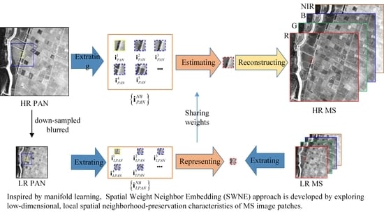
2. Spatial Weighted Neighbor Embedding (SWNE) for Image Fusion

In the following sections we will first discuss SWNE and then SWNE based image fusion method.

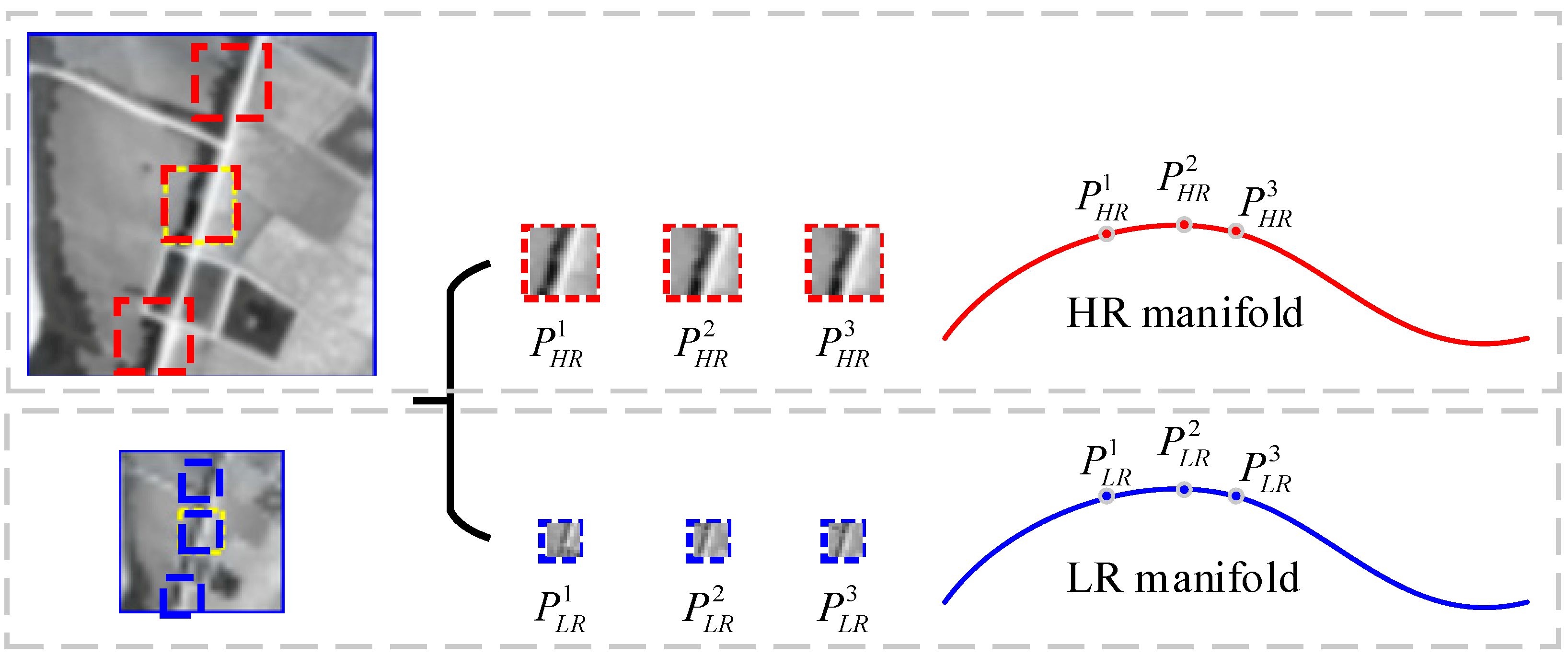
2.1. Spatial Weighted Neighbor Embedding (SWNE)

Inspired by manifold learning [37], in this section we develop a Spatial Weight Neighbor Embedding (SWNE) approach by exploring low-dimensional, local spatial neighborhood-preservation characteristics of MS image patches. In the following section we will first discuss SWNE and then SWNE based image-fusion method.

In the proposed method, the observed PAN image ${\mathbf{I}}_{PAN}$ is divided into small overlapped $\sqrt{v}\times \sqrt{v}$ patches ${\mathbf{i}}_{PAN}^k\in R^v$ $(k=1,\dots K)$, $v$ is the number of pixels in a patch. Each band of LR MS images ${\mathbf{I}}_L^p(p=R,G,B,NIR)$ is also divided into small overlapped $\sqrt{v/r^2}\times \sqrt{v/r^2}$ patches ${\mathbf{i}}_L^{p,k}\in R^{v/r^2}(p=R,G,B,NIR;k=1,\dots ,K)$. $r$ is the ratio of spatial resolution between LR MS and HR MS images. $K$ denotes the number of partitioned patches. The number of partitioned patches from the PAN image is equal to the number of patches of one band in the MS image. The number of bands in the MS image is $p$. For the bands in MS image, R, G, B and NIR stand for Red, Green, Blue and Near-Infrared. Similarly, each band of the fused HR MS images ${\mathbf{I}}_H^p(p=R,G,B,NIR)$ is divided into small overlapped patches ${\mathbf{i}}_H^{p,k}(p=R,G,B,NIR;k=1,\dots K)$. Both of the observed LR MS images patches ${\left\{{\mathbf{i}}_L^{p,k}\right\}}_{k=1}^K$ and PAN image patches ${\left\{{\mathbf{i}}_{PAN}^k\right\}}_{k=1}^K$ can be considered as the degradation results of the HR MS image patch ${\left\{{\mathbf{i}}_H^{p,k}\right\}}_{k=1}^K$, which can be written as,

$${\mathbf{i}}_L^{p,k}=H_1\left({\mathbf{i}}_H^{p,k}\right)$$

(1)

$${\mathbf{i}}_{PAN}^k=H_2\left({\mathbf{i}}_H^{p,k}\right)$$

(2)

where $H_1(\cdot )$ and $H_2(\cdot )$ denote the spatial and spectral degradation functions, respectively. For the image fusion task, the goal is to recover ${\left\{{\mathbf{i}}_H^{p,k}\right\}}_{k=1}^K$ from the observed ${\left\{{\mathbf{i}}_L^{p,k}\right\}}_{k=1}^K$ and ${\left\{{\mathbf{i}}_{PAN}^k\right\}}_{k=1}^K$.

In recent decades, manifold learning has been developed to discover low-dimensional nonlinear manifolds in high-dimensional data spaces, which have been applied to information retrieval and computer vision [38,39,40] successfully, such as neighbor embedding (NE) [38] proposed by Chang et al. [38], and local linear embedding (LLE) proposed by Roweis et al. [41,42]. As for image fusion, there are LR MS and PAN images to be merged. Although the spectral response of MS bands is different from that of the PAN image, the LR MS image patch and LR PAN image patch located at the same position will represent the same scene range for their consistent spatial resolution. Consequently, the structure of the LR MS image patch (named as a target patch) is similar to that of a set of LR PAN image patches whose spatial location is identical with or close to that of the target patch. This prior is called local structure similarity in the paper. Based on this local structure similarity prior, a new spatial weighted neighbor embedding is proposed to find more accurate embedding to recovery HR MS images.

In our method, we down-sample PAN image ${\mathbf{I}}_{PAN}$ to produce LR PAN image ${\mathbf{I}}_{LPAN}$ and consider the LR patch ${\mathbf{i}}_{LPAN}^j$ whose corresponding HR version is ${\mathbf{i}}_{PAN}^j$. The target LR MS image patches located at the same position are denoted as ${\mathbf{i}}_L^{p,j}(p=R,G,B,NIR)$. SWNE finds the nearest neighbors of ${\mathbf{i}}_L^{p,j}(p=R,G,B,NIR)$ from a local spatial neighborhood of ${\mathbf{i}}_{LPAN}^j$, to formulate a set of LR image patches $\left\{{\mathbf{i}}_{LPAN}^{j,NB}\right\}$. In SWNE, it is assumed that each image patches ${\mathbf{i}}_L^{p,j}$ and its spatial neighbors $\left\{{\mathbf{i}}_{LPAN}^{j,NB}\right\}$, are expected to lie on or close to a locally linear manifold. Moreover, their corresponding HR patches ${\mathbf{i}}_{HMS}^{p,j}$ and $\left\{{\mathbf{i}}_{PAN}^{NB}\right\}$ are assumed to share the similar manifold structure, as shown in Figure 3. Consequently, finding the atoms for representing a target patch ${\mathbf{i}}_L^{p,j}$ can be formulated as the selection of neighbors from a LR patches set $\left\{{\mathbf{i}}_{LPAN}^{j,NB}\right\}$. In SWNE, a local window is utilized to restrict the spatial locations of LR PAN patches $\left\{{\mathbf{i}}_{LPAN}^{j,NB}\right\}$. Due to the local structure similarity existing in images, it is assumed that the patches in the window partly or entirely lie in the same manifold as the target patch ${\mathbf{i}}_L^{p,j}$, and that their linear superposition can approximate ${\mathbf{i}}_{MS}^{p,j}$. That is, SWNE first finds the spatial neighbors of the LR patch. Secondly the weights of these neighbors can be estimated by the approximate error, in which the LR patch is reconstructed by these neighbors. Then, the weights of these neighbors are shared with their corresponding HR patches $\left\{{\mathbf{i}}_{PAN}^{NB}\right\}$. Finally, the HR patch ${\mathbf{i}}_H^{p,j}$ can be synthesized by the sum of HR patches $\left\{{\mathbf{i}}_{PAN}^{NB}\right\}$ multiplying with their corresponding weights.

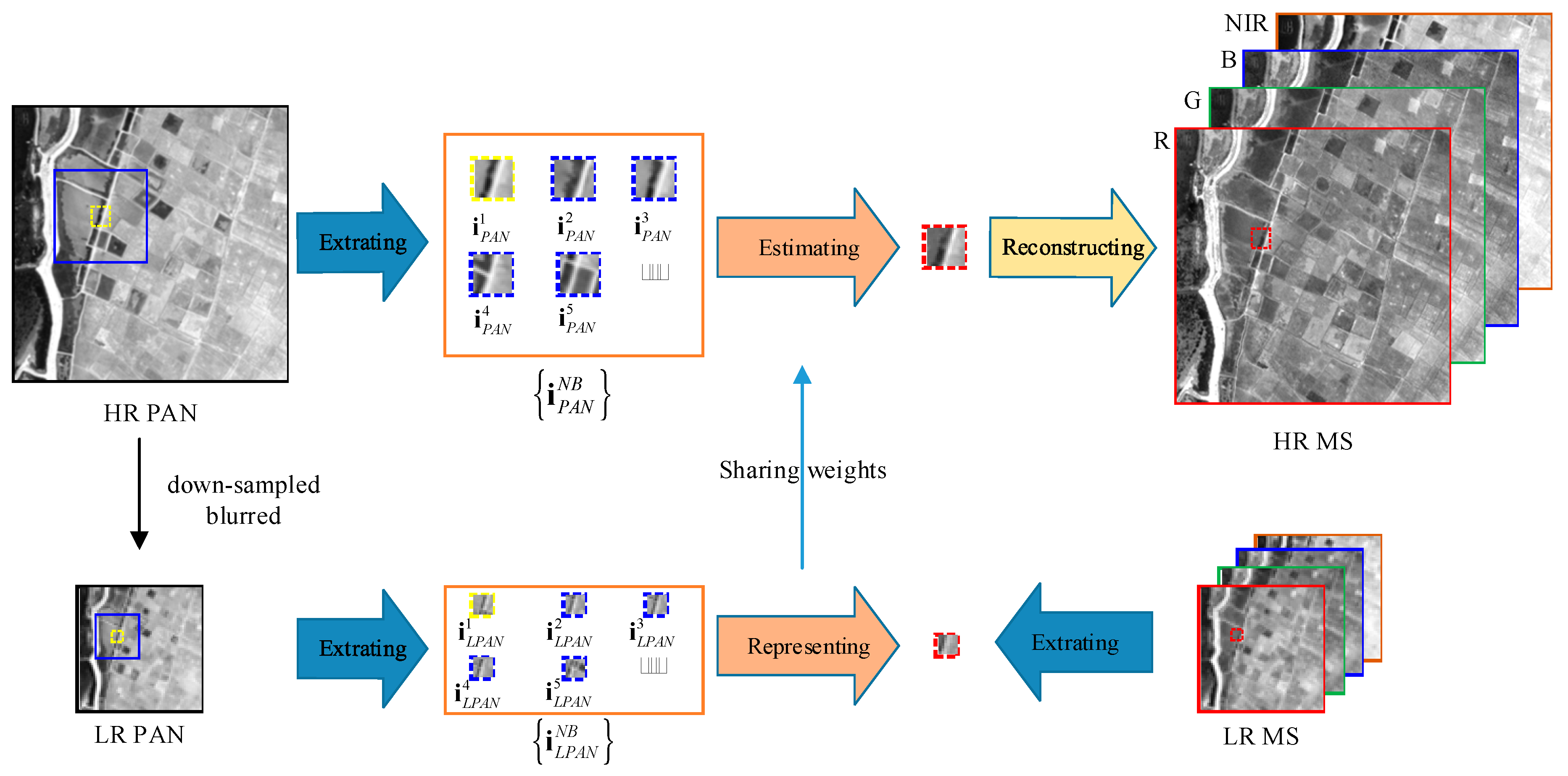
2.2. Multispectral (MS) and Panchromatic (PAN) Images Fusion Based on SWNE

Inspired by manifold learning [42], in this section we develop a SWNE approach by exploring low-dimensional, local spatial neighborhood-preservation characteristics of MS image patches. In the following section we will first discuss SWNE and then the SWNE-based image-fusion method.

The flowchart of the proposed method based on SWNE is reported in Figure 4. Firstly the observed PAN image is down-sampled by a fixed ratio $r$ to produce a LR PAN image. Secondly, the LR PAN image and the observed MS image are divided into small overlapped patches. Then, the neighbor patches found in LR PAN image patches are used to represent the LR MS image patch, in which the weight coefficients corresponding to the neighbors are estimated. Finally, the corresponding HR PAN image patches of these neighbors are multiplied with the weight coefficients whose results are added together to construct the desired HR MS image patch.

Given a LR image patch ${\mathbf{i}}_{LPAN}^j$ and its corresponding HR image patch ${\mathbf{i}}_{PAN}^j$, denoted by yellow square, as shown in Figure 4, the neighbors of a LR MS image patch ${\mathbf{i}}_L^{p,j}$ are selected from the local window in the LR PAN image, i.e., $\left\{{\mathbf{i}}_{LPAN}^{j,NB}\right\}$, to formulate a low-dimensional embedding. Selecting neighbors and evaluating weights are important in determining this low-dimensional embedding. It is obvious that there are different patches $\left\{{\mathbf{i}}_{LPAN}^{j,NB}\right\}$ in the local window, and some patches has similar structure to that of ${\mathbf{i}}_{PAN}^j$ while others should be excluded in the reconstruction of ${\mathbf{i}}_{PAN}^j$. In the proposed method, neighbors and weights are simultaneously determined. Assume that there are $N$ patches in the window, the estimation of weights can be formulated as:

$${\Vert \left[i_L^{p,j}-i_{LPAN}^1,\dots ,i_L^{p,j}-i_{LPAN}^i,\dots ,i_L^{p,j}-i_{LPAN}^N\right]w_k\Vert }_2\le \epsilon s.t.e^T{w}_k=1$$

(3)

where $\epsilon$ is the approximation error, ${\Vert \cdot \Vert }_2$ denotes the square distance; $w_k$ is a column vector of weights and $e$ is a column vector of ones with length $N$. In order to exclude the outliers, the vectors are normalized to reformulate (3) as,

$${\Vert \left[\frac{i_L^{p,j}-i_{LPAN}^1}{{\Vert i_L^{p,j}-i_{LPAN}^1\Vert }_2},\dots ,\frac{i_L^{p,j}-i_{LPAN}^i}{{\Vert i_L^{p,j}-i_{LPAN}^i\Vert }_2},\dots ,\frac{i_L^{p,j}-i_{LPAN}^N}{{\Vert i_L^{p,j}-i_{LPAN}^N\Vert }_2}\right]w_k\Vert }_2\le \epsilon s.t.e^T{w}_k=1$$

(4)

In this way, the contribution of patches which are far away from the target patch in Euclidean space is reduced, along with these patches not being identical to or similar with the target patch in spatial structure. Too many neighborhood patches will lead to the spatial distortions and blurring effects. Besides, it is not feasible to use all of the patches or a fixed number of patches in the local window [43] to represent a target patch [44], because the embedded manifold will have different curvature at different positions. Thus, the spatial structure of $i_L^{p,j}$ can be represented more reasonably by casting a weighted $L_1$ norm regularizer on the weight vector. The neighbors of each target patch can be selected from the local window adaptively. Finally, the weight optimization can be written as:

$$\{\begin{array}{l}\underset{w_k}{\min }{\Vert v\circ w_k\Vert }_1\\ s.t.{\Vert \left[\frac{i_L^{p,j}-i_{LPAN}^1}{{\Vert i_L^{p,j}-i_{LPAN}^1\Vert }_2},\dots ,\frac{i_L^{p,j}-i_{LPAN}^i}{{\Vert i_L^{p,j}-i_{LPAN}^i\Vert }_2},\dots ,\frac{i_L^{p,j}-i_{LPAN}^N}{{\Vert i_L^{p,j}-i_{LPAN}^N\Vert }_2}\right]w_k\Vert }_2\le \epsilon \\ e^T{w}_k=1\end{array}$$

(5)

where ${\Vert \cdot \Vert }_1$ is the $L_1$ norm. $v$ denotes a weighted vector and the element takes the form of $\frac{{\Vert i_L^{p,k}-i_{LPAN}^j\Vert }_2}{{\displaystyle \sum _{j=1}^N{\Vert i_L^{p,k}-i_{LPAN}^j\Vert }_2}}$. $\circ$ is the Hadamard product. In order to find the solution sufficiently, Equation (5) is optimized by the method of Lagrange multipliers. So (5) is reformulated as:

$$\{\begin{array}{l}\underset{w_k}{\min }{\Vert \left[\frac{i_L^{p,j}-i_{LPAN}^1}{{\Vert i_L^{p,j}-i_{LPAN}^1\Vert }_2},\dots ,\frac{i_L^{p,j}-i_{LPAN}^i}{{\Vert i_L^{p,j}-i_{LPAN}^i\Vert }_2},\dots ,\frac{i_L^{p,j}-i_{LPAN}^N}{{\Vert i_L^{p,j}-i_{LPAN}^N\Vert }_2}\right]w_k\Vert }_2+\lambda {\Vert v\circ w_k\Vert }_1\\ s.t.e^T{w}_k=1\end{array}$$

(6)

where $\lambda$ controls the number of neighbors. The above minimization problem is solved by the alternative direction multiplier method (ADMM) [45] in [44]. After the neighbors and their weights are determined simultaneously, the corresponding HR patch of HR MS image can be recovered from

$${\mathbf{i}}_H^{p,k}=\left[i_{PAN}^1,\dots ,i_{PAN}^j,\dots ,i_{PAN}^N\right]w_k$$

(7)

Note that the HR patch is denoted by the difference between the pixel values and the mean value of each HR patch. So the mean value of the corresponding LR patch should be added for reconstructing the target HR patch.

3. Experiments Results and Analysis

In this section, several experiments are taken to investigate the performance of the proposed method, including: (1) an investigation on the recovery result of SWNE; (2) analysis of the influence of parameter $\lambda$ on the performance of the proposed method; (3) analysis of the influences of patch size and window size on the performance of the proposed method; (4) an investigation on the fusion result of our proposed method and its counterparts.

3.1. Datasets and Experimental Conditions

The experiments were simulated on the QucikBird [46] and Geoeye-1 [47] satellite image datasets. The QuickBird image datasets used in this paper are from the Sundarbans, India, collected on 21 November 2002, which provides PAN images at 0.7 m resolution and MS images at 2.8 m resolution. The Geoeye-1 image datasets are from the Hobart, Australia, acquired on 24 February 2009. The spatial resolution of PAN images and MS images of Geoeye-1 are 0.5 m and 2 m respectively. For a comprehensive comparison, the experiments are conducted on reduced-scale and full-scale. The reduced-scale datasets are produced by down-sampling and filtering on the original LR MS images and PAN images. Therefore, the reference images are available. Then the resolution of PAN and MS images from QuickBird becomes 2.8 m and 11.2 m. Likewise, 2 m PAN and 8 m MS images are yielded from Geoeye-1. Finally, the simulated LR MS and PAN images are fused to produce HR MS image, which is compared directly with the original LR MS image according to the Wald protocol [48]. For the full-scale datasets, the fusion is implemented on the original source images and there are no reference images. Thus, the spatial resolution of the fused image is consistent with that of the original PAN image.

In subsequent experiments, the proposed method is compared with some classical methods, including generalized intensity–hue–saturation (GIHS) [49], PCA [6], proportional additive wavelet LHS (AWLP) [50], SVT [12] and SparseFI [32]. Additionally, an image-fusion method based on NE without local similarity is also reported to verify the rationality of spatial prior. The size of the LR MS images is $64\times 64\times 4$. Correspondingly, the size of PAN image is $256\times 256$. In order to enforce smoothness constraints between adjacent patches, proper parameters have to be preset, such as LR MS patch size and degree of overlap. We use $3\times 3$ patches with an overlap of 2 pixels in the proposed method and NE. The size of the window in the LR PAN image is set as $7\times 7$. Each target patch can select their neighbors from 25 patches in the local window. $\lambda$ is set as 60 and 50 for QucikBird and Geoeye-1 satellite image datasets, respectively. In NE, the number of neighbors is 5 and the first- and second-order gradient feature is used to choose neighbors. Besides, the LR and HR patch sets are constructed by the LR and HR PAN images. SparseFI adopts the parameters recommended in [32] and the patch size and overlap size are $7\times 7$ and $7\times 3$, respectively.

3.2. Evaluation Indexes

In order to evaluate the quality of fused images on different datasets, some indicators are calculated such as correlation coefficient (CC) [51], frequency comparison (FC) [52], Q4 [51], Erreur relative globale adimensionnelle de synthèse (ERGAS) [53], spectral angle mapper (SAM) [54]. These indicators are selected to assess the quality of the fused image from two perspectives: spatial information and spectral information. CC reflects the correlation between two single bands from the fused image and the reference image. Q4 is used to measure the spectral distortion of fused images compared with the reference image. ERGAS computes the spectral distortion in the image from the whole. SAM calculates the angle between the corresponding pixels of the fused and the reference images to measure the spectral distortions. FC evaluates the spatial details of the fused images. Among the five indexes, CC, FC and Q4 indicate better fusion results as they increase in the interval $[0,1]$, whose ideal values are 1. For ERGAS and SAM, a better result is indicated by a smaller value. The fusion results of full-scale datasets are assessed by $D_{\lambda }$, $D_S$ and QNR [55]. For QNR, the best value is 1. But the best value is 0 for $D_{\lambda }$ and $D_S$. Then, the above evaluation indexes are utilized to numerically and quantitatively assess the fused images of all methods.

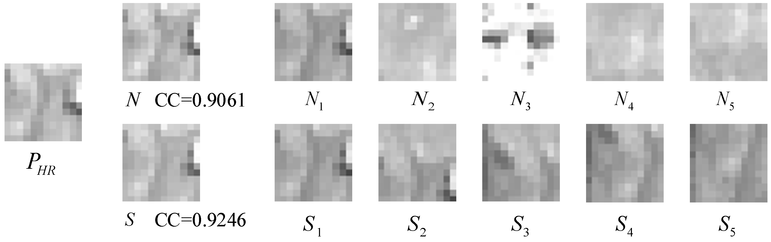
3.3. Investigation of SWNE

In this test, we compare the HR neighbors found by NE and SWNE. The NE selects the LR and HR neighbors from the sets constructed by the LR and HR PAN images, respectively. A $12\times 12$ target HR patch $P_{HR}$ is illustrated as an example. Figure 5 displays the neighbors $\left\{N_1,\dots ,N_5\right\}$ that are found from the HR patch set in NE method, and the neighbors $\left\{S_1,\dots ,S_5\right\}$ found by the SWNE method.

From Figure 5, it can be found that the neighbors $\left\{N_2,\dots ,N_5\right\}$ are very different with the target patch, because a global searching can find the nearest neighbors in Euclidean distance but the structural similarity cannot be guaranteed. We can see that the neighbors are more similar in structure and the Euclidean distance varies in an acceptable range simultaneously in $\left\{S_2,\dots ,S_5\right\}$. Therefore, these more reliable neighbors can provide a smaller bias to the image reconstruction, which will sharpen the spatial details. Besides, the target HR patches $N$ and $S$ are reconstructed by the neighbors from NE and SWNE, respectively. It is obvious that the patch $S$ is more similar to the patch $P_{HR}$ and provides a larger CC.

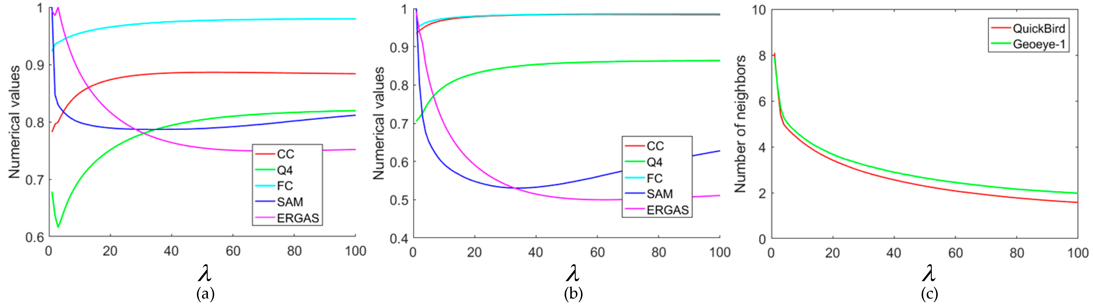
3.4. Investigation of $\lambda$

The parameter $\lambda$ controls the number of neighbors, which balances the spectral and spatial fidelity. In this experiment, we take the QuickBird image datasets and Geoeye-1 image datasets as examples to analyze how the parameter $\lambda$ affects the fusion results in different datasets. We use $3\times 3$ patches with an overlap of 2 pixels to implement the proposed method, and the local window is also portioned into patches in the same way. So there are 25 patches in a window with size $7\times 7$. The variations of all metrics on the QuickBird and Geoeye-1 image datasets is illustrated in Figure 6a,b, respectively. The values of ERGAS and SAM are normalized to $[0,1]$ for direction comparison. Figure 6a shows that CC, Q4 and FC increase and the other two metrics decrease with $\lambda$ increasing in $[0,60]$. In Figure 6a, SAM decreases with increasing $\lambda$. For ERGAS, it decreases dramatically first and then slowly increases. Unfortunately, the best values of ERGAS and SAM cannot be achieved on the same $\lambda$. Naturally, we have to choose a compromise value for $\lambda$ taking the tradeoff between SAM and ERGAS into consideration. Therefore, $\lambda$ is set as 60 by taking the overall performance of the proposed method for QuickBird image datasets. Similarly, the same trend of metrics can be found in Figure 6b. So $\lambda$ is set as 60 and 50 for the datasets from QuickBird and Geoeye-1 satellites, empirically. Besides, the average number of neighbors is computed for different $\lambda$, which is shown in Figure 6c. The decrease in the number of neighbors can be observed with $\lambda$ increasing. Only a few patches are used to denote the target. For a large number of neighbors, SWNE performs badly in terms of all metrics due to the use of some dissimilar patches. In fact, it implies most elements of the weight vector $w_k$ taking values close to zero while only few take significantly non-zero values. However, if only very limited patches are utilized, the spectral information will be reduced. Thus, SWNE can select adaptively the most similar neighbors to represent the target patch, which enhances the spatial details.

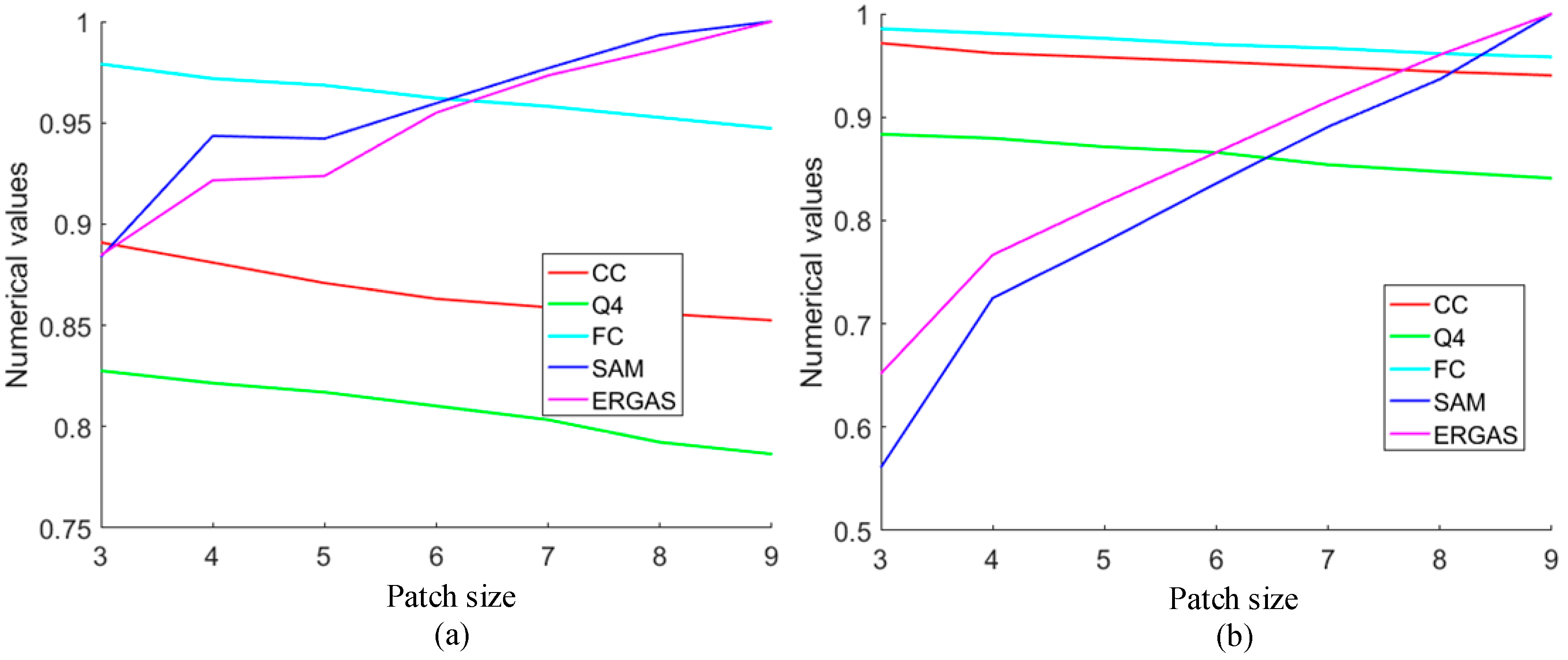
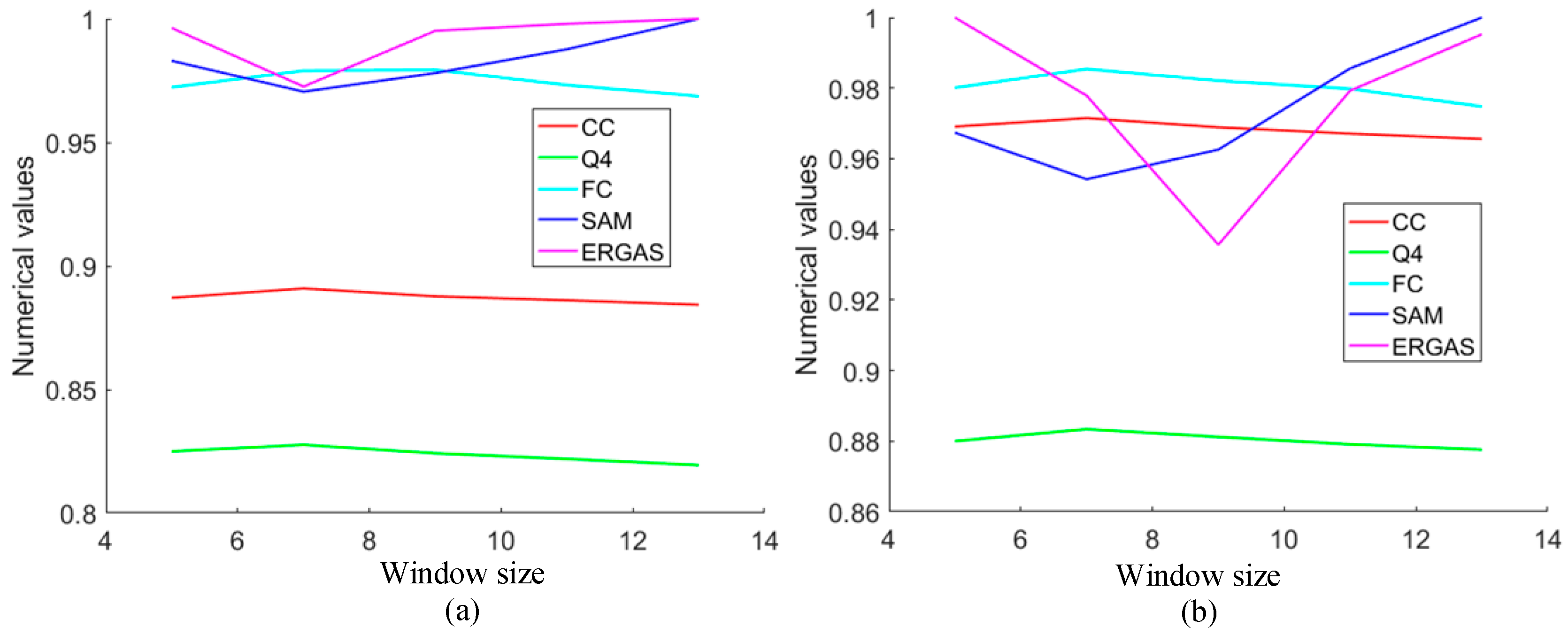
3.5. Investigation of Patch Size and Window Size

In the proposed method, patch size and window size have some influences on fusion results. We analyze the influences of patch size and window size on QuickBird and Geoeye-1 image datasets in this section. The numerical values of all indexes are displayed in Figure 7, where patch size varied from 3 to 9 with step 1. From, Figure 7a,b, we can see that the values of CC, Q4 and FC gradually decrease and SAM and ERGAS increase, which means the quality of fused images becomes worse. So, the patch size is set as $3\times 3$. In Figure 8, the influences of different window sizes are shown, in which window size varies from 5 to 13 with step 2. It can be observed that the best values of CC, Q4, SAM and ERGAS indexes are given in Figure 8a when the window size is $7\times 7$. For FC, competitive results are produced for windows with size $7\times 7$ and $9\times 9$. Therefore, the window size is set as $7\times 7$ for QuickBird image datasets by considering the overall performance. In Figure 8b, the best ERGAS is obtained with $9\times 9$ window, but the values of other indexes are achieved when the window size is $7\times 7$. For windows with larger size, the number of neighbor candidates is larger. Therefore, it is difficult to find accurate neighbor patches with a larger size window. However, the target patch cannot be represented effectively for fewer neighbors in the window with small size. Thus, the window size is set as $7\times 7$.

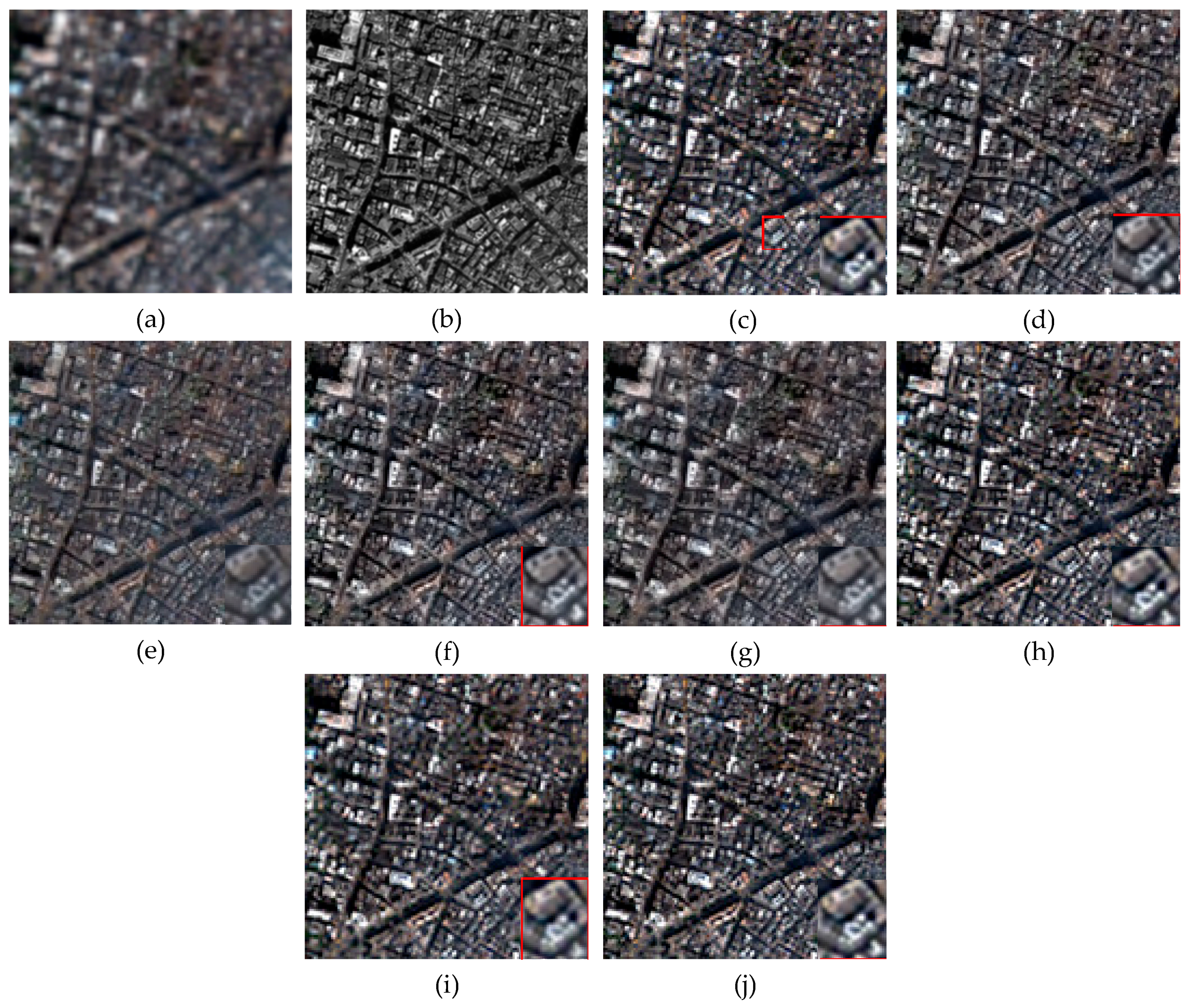
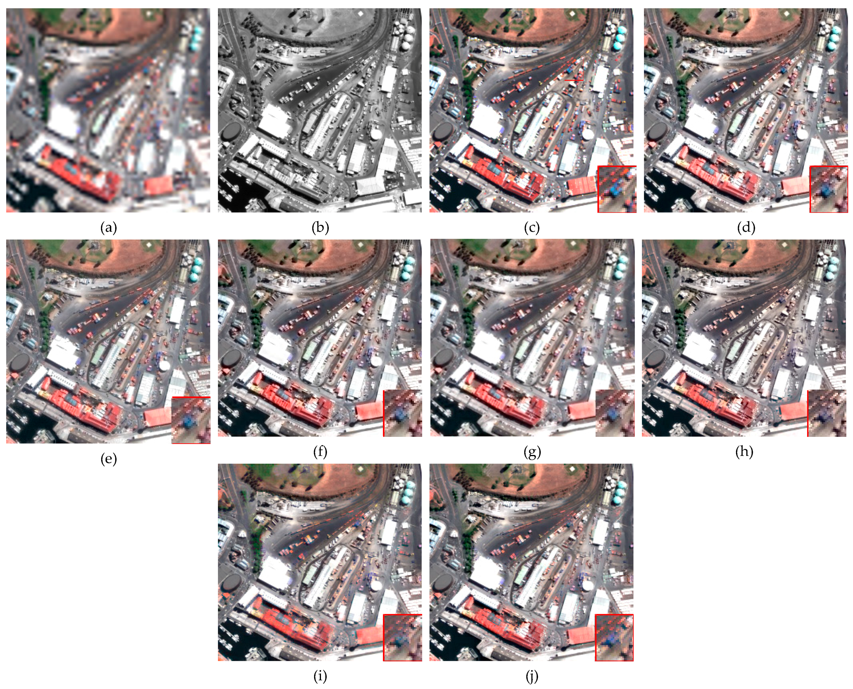
3.6. Experiments on Reduced-Scale Datasets

In this part, experiments were conducted on reduced-scale datasets. Two pairs of images from Quickbird and Geoeye-1 satellites are fused and the fusion results are compared with GIHS [49], PCA [6], AWLP [50], SVT [12] and SparseFI [32]. The experimental results of these methods on QuickBird image dataset are shown in Figure 9d–j. The source images to be fused are given in Figure 9a,b. The reference images are displayed in Figure 9c for visual comparison. It can be seen that the fusion results of all methods always have some differences compared with the reference images. For spatial details, the result of GIHS [49] behaves well, but some blur effects can be found in the result of PCA [6]. For MRA-based methods, AWLP [50] can provide clear spatial details but the spatial information is blurred in the result of SVT [12]. The spatial details in SparseFI [32], NE and SWNE are similar. For spectral information, obvious spectral distortions can be found in the results of PCA [6], AWLP [50] and SVT [12]. GIHS [49] can preserve the spectral information in the fused image well. NE and SWNE also can produce better results in spectral information preservation. However, the spectral information of the result of SparseFI [32] is more consistent with that of the reference image through visual comparison.

Table 1. Numerical results of each fused image shown in Figure 9.

Metric	GIHS [49]	PCA [6]	AWLP [50]	SVT [13]	SparseFI [32]	NE	SWNE
CC	0.8700	0.8563	0.8642	0.8705	0.8798	0.8830	0.8909
Q4	0.8187	0.6741	0.8019	0.7932	0.8328	0.7943	0.8276
FC	0.9730	0.9701	0.9778	0.9713	0.9750	0.9759	0.9790
SAM	9.7731	9.8995	10.6052	9.7133	9.4060	9.2355	9.1420
ERGAS	4.3984	5.3566	4.4717	4.4366	4.1915	4.2329	4.0089

reports the numerical results in Figure 9 and the best results for each quality metric are labeled in bold. We can see that the proposed method provides almost the best values in term of metrics CC, FC, SAM, and ERGAS. SWNE behaves best, followed by NE and SparseFI [32] in ERGAS. The value of FC is the best for the proposed method, which means the fusion result provides the best spatial quality. The proposed method also provides the best result in SAM. Q4 mainly reflects the spectral distortion of fused images. Larger Q4 means less spectral distortion. The proposed method is preferable to the other methods except SparseFI [32] for the Q4 index, which agrees with the analysis in Figure 9. The proposed method has a better performance as a whole.

The fusion results of all methods on Geoeye-1 image datasets are illustrated in Figure 10. The differences of all fused images are small by a visual comparison of spatial details. However, some differences can be found when all fused images are compared with the reference image especially in spectral information. From the magnified region, we can see that the spectral information in the results of AWLP [50], SVT [12] and SparseFI [32] are distorted obviously when compared with other methods by subjective visual analysis.

For more objective evaluation in spatial and spectral information, the numerical values are listed in

Table 2. Numerical results of each fused image shown in Figure 10.

Metric	GIHS [49]	PCA [6]	AWLP [50]	SVT [12]	SparseFI [32]	NE	SWNE
CC	0.9670	0.9632	0.9687	0.9693	0.9699	0.9691	0.9715
Q4	0.8939	0.8571	0.8965	0.8982	0.9021	0.8783	0.8834
FC	0.9798	0.9718	0.9850	0.9839	0.9791	0.9841	0.9854
SAM	4.1535	3.4104	4.7313	4.4978	4.2024	4.2186	4.0642
ERGAS	1.6761	1.7801	1.5507	1.5272	1.5033	1.5437	1.4631

. From the table, a competitive result can be seen. For CC, the proposed method gives the best values. For FC, the best value is from the proposed method and the second best FC is produced by AWLP. As for SAM, the best results are given by PCA [6], followed by AWLP [50] in Table 2. For Q4, SparseFI [32] offers the best results in the table. However, SWNE outperforms the other methods in ERGAS. The proposed method behaves well in CC and ERGAS.

3.7. Experiments on Full-Scale Datasets

In this part, two pairs of images at full scale from Quickbird and Geoeye-1 satellites are used for fusion and then the fused images of the proposed method are compared with those of GIHS [49], PCA [6], AWLP [50], SVT [12] and SparseFI [32]. The fusion results of all methods on QuickBird image datasets are illustrated in Figure 11. From Figure 11, we can see that the spatial details of all methods are enhanced well when compared with the LR MS image. However, obvious spectral information loss can be found from the result of PCA [6], in which the color of some areas is transformed into blue. The color of tree areas becomes grayish-green in the results of GIHS [49] and SVT [12]. Through subjective visual comparison, other methods have a comparable performance in spectral information preservation.

Besides, for more objective assessment of fusion results, the numerical results of all methods in Figure 11 are given in

Table 3. Numerical results of each fused image shown in Figure 1.

Metric	GIHS [49]	PCA [6]	AWLP [50]	SVT [12]	SparseFI [32]	NE	SWNE
FC	0.9519	0.9508	0.9679	0.9662	0.9599	0.9565	0.9690
$D_{\lambda }$	0.0820	0.0875	0.0669	0.0659	0.0476	0.0784	0.0838
$D_S$	0.0909	0.0977	0.0777	0.0843	0.0976	0.0678	0.0609
QNR	0.8346	0.8322	0.8606	0.8562	0.8594	0.8591	0.8604

. From Table 3, we can see that the best values of FC and $D_S$ are from SWNE. But the value of $D_{\lambda }$ of the proposed method is poor. Although, the best QNR is given by AWLP [49], but the second best value of QNR is achieved by the proposed method.

The fusion results on Geoeye-1 image dataset are displayed in Figure 12. From Figure 12, it can be observed that the spectral information of fused images from all methods is not consistent. The color of tree areas in the result of GIHS [49] and PCA [6] is dark green and some tree areas are over-enhanced in edges. For AWLP [50] and SVT [12], the color of tree areas is bright green and the spectral information of some buildings is distorted slightly. However, the color of tree areas is grayish-green for SparseFI [32], NE and SWNE. For the result of SparseFI, there are some spectral distortions for the color of road areas. Due to the unavailable reference image in full-scale datasets, it is difficult to analyze directly the spectral information in the fused images of all methods.

Therefore, the numerical evaluation results of all methods are listed in

Table 4. Numerical results of each fused image shown in Figure 12.

Metric	GIHS [49]	PCA [6]	AWLP [50]	SVT [12]	SparseFI [32]	NE	SWNE
FC	0.9436	0.9495	0.9576	0.9561	0.9557	0.9532	0.9569
$D_{\lambda }$	0.0944	0.1021	0.1295	0.1286	0.1086	0.1168	0.1071
$D_S$	0.1213	0.0892	0.0785	0.0567	0.0587	0.0628	0.0525
QNR	0.7957	0.8178	0.8022	0.8220	0.8390	0.8277	0.8460

for objective analysis. In Table 4, the fusion result of AWLP behaves best in FC. The second best FC is produced by the proposed method and the difference between AWLP and the proposed method SWNE is small for FC. Besides, the best value $D_{\lambda }$ is from GIHS [49], but the proposed method SWNE has the best performance in $D_S$ and QNR. Thus, the proposed method behaves better as a whole.

4. Conclusions

In this paper, an image-fusion method based on SWNE is proposed to obtain an HR MS image by merging the LR MS and PAN images. The local geometry of LR MS image patch over the neighbors is explored to develop a spatial low-dimensional embedding. HR image patches are then estimated by combining a few candidate HR patches selected from a neighborhood region. The reconstruction weights of HR neighbors are estimated by solving a weighted problem that is solved by ADMM to exclude some outliers. In the proposed method, patch size and window size play an important in fusion performance. An image patch with small size can efficiently capture the spatial and spectral information. The window with larger size has a great number of patches, but it is difficult to find accurate neighbors. Inversely, the window with small size has a limited representation ability because of fewer patches. $\lambda$ decides the number of neighbors. Larger $\lambda$ will select fewer neighbors to reconstruct the target patch, which is more likely to cause spectral distortion. Smaller $\lambda$ allows more neighbors for fusion, which may lead to smooth spatial information. Finally, the proposed method is compared with other image fusion methods on QuickBird and Geoeye-1 satellite image datasets. The experimental results show that the proposed method behaves better than other methods in spatial enhancement and spectral preservation. Although the proposed method produces some satisfactory fusion results, the time complexity cannot be ignored because the optimization of the proposed method is achieved by ADMM with a lot of iterations. Besides, noises in source images have certain influence on the selection of neighbor patches. The noises may result in the changes of structures in image patches. Thus, similar neighbor patches in spatial structure cannot be chosen. Therefore, a more efficient selection scheme of neighbor patches, such as in [56], will be considered in the future work to mitigate the issues about running time and noise.

References

1. Ji, S.; Wei, S.; Lu, M. Fully convolutional networks for multisource building extraction from an open aerial and satellite imagery data set. IEEE Trans. Geosci. Remote Sens. 2019, 57, 574–586. [Google Scholar] [CrossRef]
2. Wu, X.; Zhang, X.; Wang, N.; Cen, Y. Joint sparse and low-rank multi-task learning with extended multi-attribute profile for hyperspectral target detection. Remote Sens. 2019, 11, 150. [Google Scholar] [CrossRef]
3. Yin, H. Sparse representation based pansharpening with details injection model. Signal Process. 2015, 113, 218–227. [Google Scholar] [CrossRef]
4. Javan, F.D.; Samadzadegan, F.; Reinartz, P. Spatial quality assessment of pan-sharpened high resolution satellite imagery based on an automatically estimated edge based metric. Remote Sens. 2013, 5, 6539–6559. [Google Scholar] [CrossRef]
5. Vivone, G.; Alparone, L.; Chanussot, J.; Mura, D.M.; Garzelli, A.; Licciardi, A.G.; Restaino, R.; Wald, L. A critical comparison among pansharpening algorithms. IEEE Trans. Geosci. Remote Sens. 2015, 53, 2565–2586. [Google Scholar] [CrossRef]
6. Chavez, P.S.; Sides, S.C.; Anderson, J.A. Comparison of three different methods to merge multiresolution and multispectral data: Landsat TM and SPOT Panchromatic. Photogramm. Eng. Remote Sens. 1991, 57, 265–303. [Google Scholar]
7. Laben, C.A.; Brower, B.V. Process for Enhancing the Spatial Resolution of Multispectral Imagery Using Pan-Sharpening, Eastman Kodak Company. U.S. Patent 6011875, 4 January 2000. [Google Scholar]
8. Tu, T.M.; Su, S.C.; Shyu, H.C.; Huang, P.S. A new look at IHS-like image fusion methods. Inf. Fusion 2012, 3, 177–186. [Google Scholar] [CrossRef]
9. Strait, R.S.; Merkurjev, M.D.; Moeller, M.; Wittman, T. An adaptive IHS pan-sharpening method. IEEE Geosci. Remote Sens. Lett. 2010, 7, 746–750. [Google Scholar]
10. Ranchin, T.; Aiazzi, B.; Alparone, L.; Baronti, S.; Wald, L. Image fusion—The ARSIS concept and some successful implementation schemes. ISPRS J. Photogramm. Remote Sens. 2003, 58, 4–18. [Google Scholar] [CrossRef]
11. Pradhan, P.S.; King, R.L.; Younan, N.H.; Holcomb, D.W. Estimation of the number of decomposition levels for a wavelet-based multiresolution multisensor image fusion. IEEE Trans. Geosci. Remote Sens. 2006, 44, 3674–3686. [Google Scholar] [CrossRef]
12. Zheng, S.; Shi, W.Z.; Liu, J.; Tian, J. Remote sensing image fusion using multiscale mapped LS-SVM. IEEE Trans. Geosci. Remote Sens. 2008, 46, 1313–1322. [Google Scholar] [CrossRef]
13. Shah, V.P.; Younan, N.H.; King, R.L. An efficient pan-sharpening method via a combined adaptive PCA approach and contourlets. IEEE Trans. Geosci. Remote Sens. 2008, 46, 1323–1335. [Google Scholar] [CrossRef]
14. Kahaki, S.M.M.; Jan, N.M.; Ashtari, A.H.; Zahra, J.S. Deformation invariant image matching based on dissimilarity of spatial features. Neurocomputing 2016, 175, 1009–1018. [Google Scholar] [CrossRef]
15. Garzelli, A.; Aiazzi, B.; Alparone, L.; Lolli, S.; Vivone, G. Multispectral pansharpening with radiative transfer-based detail-injection modeling for preserving changes in vegetation cover. Remote Sens. 2018, 10, 1308. [Google Scholar] [CrossRef]
16. Wang, W.; Jiao, L.; Yang, S. Fusion of multispectral and panchromatic images via sparse representation and local autoregressive model. Inf. Fusion 2014, 20, 73–87. [Google Scholar] [CrossRef]
17. Zhang, L.; Shen, H.; Gong, W.; Zhang, H. Adjustable model-based fusion method for multispectral and panchromatic images. IEEE Trans. Syst. Man Cybern. B Cybern. 2012, 42, 1693–1704. [Google Scholar] [CrossRef] [PubMed]
18. Zhang, K.; Wang, M.; Yang, S.; Xing, Y.; Qu, R. Fusion of panchromatic and multispectral images via coupled sparse non-negative matrix factorization. IEEE J. Sel. Top. Appl. Earth Obs. Remote Sens. 2016, 9, 5740–5747. [Google Scholar] [CrossRef]
19. Li, S.; Yang, B. A new pan-sharpening method using a compressed sensing technique. IEEE Trans. Geosci. Remote Sens. 2011, 49, 736–746. [Google Scholar] [CrossRef]
20. Li, S.; Yin, H.; Fang, L. Remote sensing image fusion via sparse representations over learned dictionaries. IEEE Trans. Geosci. Remote Sens. 2013, 51, 4779–4789. [Google Scholar] [CrossRef]
21. Yin, H. A joint sparse and low-rank decomposition for pansharpening of multispectral images. IEEE Trans. Geosci. Remote Sens. 2017, 55, 4779–4789. [Google Scholar] [CrossRef]
22. Yang, S.; Zhang, K.; Wang, M. Learning low-rank decomposition for pan-sharpening with spatial-spectral offsets. IEEE Trans. Neural Netw. Learn. Syst. 2018, 29, 3647–3657. [Google Scholar] [PubMed]
23. Schultz, R.R.; Stevenson, R.L. Extraction of high-resolution frames from video sequences. IEEE Trans. Image Process. 1996, 5, 996–1011. [Google Scholar] [CrossRef] [PubMed]
24. Donoho, D.L. Compressed sensing. IEEE Trans. Inf. Theory 2006, 52, 1289–1306. [Google Scholar] [CrossRef]
25. Xue, J.; Zhao, Y.; Liao, W.; Chan, J.-W. Nonlocal tensor sparse representation and low-rank regularization for hyperspectral image compressive sensing reconstruction. Remote Sens. 2019, 11, 193. [Google Scholar] [CrossRef]
26. Ying, H.; Leung, Y.; Cao, F.; Fung, T.; Xue, J. Sparsity-based spatiotemporal fusion via adaptive multi-band constraints. Remote Sens. 2018, 10, 1646. [Google Scholar] [CrossRef]
27. Zhang, Y.; Wang, X.; Xie, X.; Li, Y. Salient object detection via recursive sparse representation. Remote Sens. 2018, 10, 652. [Google Scholar] [CrossRef]
28. Zhou, Z.; Wang, M.; Cao, Z.; Pi, Y. SAR image recognition with monogenic scale selection-based weighted multi-task joint sparse representation. Remote Sens. 2018, 10, 504. [Google Scholar] [CrossRef]
29. Yang, J.; Wright, J.; Huang, T.; Ma, Y. Image super-resolution via sparse representation. IEEE Trans. Image Process. 2010, 19, 2861–2873. [Google Scholar] [CrossRef] [PubMed]
30. Gao, D.; Hu, Z.; Ye, R. Self-dictionary regression for hyperspectral image super-resolution. Remote Sens. 2018, 10, 1574. [Google Scholar] [CrossRef]
31. Zhang, K.; Wang, M.; Yang, S.; Jiao, L. Convolution structure sparse coding for fusion of panchromatic and multispectral images. IEEE Trans. Geosci. Remote Sens. 2019, 57, 1117–1130. [Google Scholar] [CrossRef]
32. Zhu, X.X.; Bamler, R. A sparse image fusion algorithm with application to pan-sharpening. IEEE Trans. Geosci. Remote Sens. 2013, 51, 2827–2836. [Google Scholar] [CrossRef]
33. Zhu, X.X.; Grohnfeldt, C.; Bamler, R. Exploiting joint sparsity for pansharpening: The J-SparseFI algorithm. IEEE Trans. Geosci. Remote Sens. 2016, 54, 2664–2681. [Google Scholar] [CrossRef]
34. Jiang, C.; Zhang, H.; Shen, H.; Zhang, L. Two-step sparse coding for the pan-sharpening of remote sensing images. IEEE J. Sel. Top. Appl. Earth Obs. Remote Sens. 2014, 7, 1792–1805. [Google Scholar] [CrossRef]
35. Wang, M.; Zhang, K.; Pan, X.; Yang, S. Sparse tensor neighbor embedding based pan-sharpening via N-way block pursuit. Knowl. Based Syst. 2018, 149, 18–33. [Google Scholar] [CrossRef]
36. Caiafa, C.; Cichocki, A. Block sparse representations of tensors using Kronecker bases. IEEE Trans. Geosci. Remote Sens. 2012, 7, 1–5. [Google Scholar]
37. Lin, T.; Zha, H. Riemannian manifold learning. IEEE Trans. Pattern Anal. Mach. Intell. 2008, 30, 796–807. [Google Scholar] [PubMed]
38. Chang, H.; Yeung, D.; Xiong, Y. Super-resolution through neighbor embedding. In Proceedings of the 2004 IEEE Computer Society Conference on Computer Vision and Pattern Recognition (CVPR 2004), Washington, DC, USA, 27 June–2 July 2004; pp. 1–9. [Google Scholar]
39. Zhang, K.; Wang, M.; Yang, S. Multispectral and hyperspectral image fusion based on group spectral embedding and low-rank factorization. IEEE Trans. Geosci. Remote Sens. 2017, 55, 1363–1371. [Google Scholar] [CrossRef]
40. Sun, L.; Zhan, T.; Wu, Z.; Xiao, L.; Jeon, B. Hyperspectral mixed denoising via spectral difference-induced total variation and low-rank approximation. Remote Sens. 2018, 10, 1956. [Google Scholar] [CrossRef]
41. Roweis, S.T.; Saul, L.K. Nonlinear dimensionality reduction by locally linear embedding. Science 2000, 290, 2323–2326. [Google Scholar] [CrossRef] [PubMed]
42. Saul, L.K.; Roweis, S.T. Think globally, fit locally: Unsupervised learning of low dimensional manifolds. J. Mach. Learn. Res. 2003, 4, 119–155. [Google Scholar]
43. Yu, H.; Gao, L.; Liao, W.; Zhang, B. Group Sparse representation based on nonlocal spatial and local spectral similarity for hyperspectral imagery classification. Sensors 2018, 18, 1695. [Google Scholar] [CrossRef] [PubMed]
44. Ehsan, E.; Vidal, R. Sparse manifold clustering and embedding. In Proceedings of the Advances in Neural Information Processing Systems 24 (NIPS 2011), Granada, Spain, 12–15 December 2011; pp. 1–9. [Google Scholar]
45. Boyd, S.; Parikh, N.; Chu, E.; Peleato, B.; Eckstein, J. Distributed optimization and statistical learning via the alternating direction method of multipliers. Found. Treads Mach. Learn. 2011, 3, 1–122. [Google Scholar] [CrossRef]
46. Kahaki, S.M.M.; Arshad, H.; Nordin, M.J.; Ismail, W. Geometric feature descriptor and dissimilarity-based registration of remotely sensed imagery. PLoS ONE 2018, 13, 0200676. [Google Scholar] [CrossRef] [PubMed]
47. Fraser, C.; Ravanbakhsh, M. Georeferencing performance of Geoeye-1. Photogramm. Eng. Remote Sens. 2009, 75, 634–638. [Google Scholar]
48. Wald, L.; Ranchin, T.; Mangolini, M. Fusion of satellite images of different spatial resolutions: Assessing the quality of resulting images. Photogramm. Eng. Remote Sens. 1997, 63, 691–699. [Google Scholar]
49. Tu, T.M.; Huang, P.S.; Hung, C.L.; Chang, C.P. A fast Intensity–Hue–Saturation fusion technique with spectral adjustment for IKONOS imagery. IEEE Geosci. Remote Sens. Lett. 2004, 1, 309–312. [Google Scholar] [CrossRef]
50. Otazu, X.; Audicana, G.M.; Nunez, J. Introduction of sensor spectral response into image fusion methods. Application to wavelet-based methods. IEEE Trans. Geosci. Remote Sens. 2005, 43, 2376–2385. [Google Scholar] [CrossRef] [Green Version]
51. Alparone, L.; Baronti, S.; Garzelli, A.; Nencini, F. A global quality measurement of pan-sharpened multispectral imagery. IEEE Geosci. Remote Sens. Lett. 2004, 1, 313–317. [Google Scholar] [CrossRef]
52. Rodriguez-Esparragon, D.; Marcello-Ruiz, J.; Medina-Machín, A.; Eugenio-Gonzalez, F.; Gonzalo-Martín, C.; Garcia-Pedrero, A. Evaluation of the performance of spatial assessments of pansharpened images. In Proceedings of the IEEE Geoscience and Remote Sensing Symposium (IGARSS), Quebec City, QC, Canada, 13–18 July 2014; pp. 1619–1622. [Google Scholar]
53. Wang, Z.; Bovik, A.C. A universal image quality index. IEEE Signal Process. Lett. 2002, 9, 81–84. [Google Scholar] [CrossRef]
54. Yuhas, R.H.; Goetz, A.F.H.; Boardman, J.W. Discrimination among semi-arid landscape endmembers using the spectral angle mapper (SAM) algorithm. In Proceedings of the 4th JPL Airborne Earth Science Workshop, Pasadena, CA, USA, 1–5 June 1992; pp. 147–149. [Google Scholar]
55. Alparone, L.; Aiazzi, B.; Baronti, S.; Garzelli, A.; Nencini, F.; Selva, M. Multispectral and panchromatic data fusion assessment without reference. Photogramm. Eng. Remote Sens. 2008, 74, 193–200. [Google Scholar] [CrossRef]
56. Xiao, C.; Liu, M.; Nie, Y.; Dong, Z. Fast exact nearest patch matching for patch-based image editing and processing. IEEE Trans. Vis. Comput. Graph. 2011, 17, 1122–1134. [Google Scholar] [CrossRef] [PubMed]
Figure 1. Mismatch of coding pattern in HR/LR spaces. Because the mismatch of manifolds between HR/LR patches, the neighbors found for LR patches cannot be consistent with the neighbors for HR patches.
Remotesensing 11 00557 g001
Figure 2. The one-to-many relationship between the low spatial-resolution (LR) patch and high spatial-resolution (HR) patches. The same LR patch can be produced by the HR patches with different geometric structures through the same spatial degradation model.
Remotesensing 11 00557 g002
Figure 3. The manifold of HR and LR patches.
Remotesensing 11 00557 g003
Figure 4. The flowchart of the proposed spatial weighted neighbor embedding (SWNE) method. The proposed method consists of five steps: (1) Produce LR panchromatic (PAN) image from HR PAN image; (2) Divide the images into patches; (3) Find the neighbors from LR PAN patches of target LR MS patch; (4) Estimate the weight of each neighbor; (5) Multiply these weights with the corresponding HR PAN patches to reconstruct HR MS patch.
Remotesensing 11 00557 g004
Figure 5. Neighbors found by neighbor embedding (NE) and SWNE. The target HR patches N and S are reconstructed by the corresponding neighbors found by NE and SWNE and then the reconstruction performance is evaluated by correlation coefficient (CC) compared with the reference patch P H R .
Remotesensing 11 00557 g005
Figure 6. The variations of metrics and neighbors with different λ . (a) Performance influence of λ on QuickBird image datasets, (b) Performance influence of λ on Geoeye-1 image datasets, (c) Variations of neighbors with different λ on QuickBird and Geoeye-1 image datasets.
Remotesensing 11 00557 g006
Figure 7. The variations of metrics with different patch size. (a) Performance influence of patch size on QuickBird image datasets, (b) Performance influence of patch size on Geoeye-1 image datasets.
Remotesensing 11 00557 g007
Figure 8. The variations of metrics with different window size. (a) Performance influence of window size on QuickBird datasets, (b) Performance influence of window size on Geoeye-1 datasets.
Remotesensing 11 00557 g008
Figure 9. Fusion results of reduced-scale QuickBird images. (a) LR MS image, (b) PAN image, (c) reference image, (d) GIHS [49], (e) principal component analysis (PCA) [6], (f) AWLP [50], (g) support value transform (SVT) [12], (h) SparseFI [32], (i) NE, (j) SWNE.
Remotesensing 11 00557 g009
Figure 10. Fusion results of reduced-scale Geoeye-1 images. (a) LR MS image, (b) PAN image, (c) reference image, (d) GIHS [49], (e) PCA [6], (f) AWLP [50], (g) SVT [12], (h) SparseFI [32], (i) NE, (j) SWNE.
Remotesensing 11 00557 g010
Figure 11. Fusion results of full-scale QuickBird images. (a) LR MS image, (b) PAN image, (c) GIHS [49], (d) PCA [6], (e) AWLP [50], (f) SVT [12], (g) SparseFI [32], (h) NE, (i) SWNE.
Remotesensing 11 00557 g011
Figure 12. Fusion results of full-scale Geoeye-1 images. (a) LR MS image, (b) PAN image, (c) GIHS [49], (d) PCA [6], (e) AWLP [50], (f) SVT [12], (g) SparseFI [32], (h) NE, (i) SWNE.
Remotesensing 11 00557 g012