Leveraging Machine Learning to Extend Ontology-Driven Geographic Object-Based Image Analysis (O-GEOBIA): A Case Study in Forest-Type Mapping


Abstract
1. Introduction
- Why is multi-sensor data fusion necessary in O-GEOBIA?
- How can spatial features be incorporated for accurate classification in O-GEOBIA?
- How can relevant features be extracted to construct rules required when identifying classes for O-GEOBIA?
- How can semantic similarity be used to characterise thematic classes in an ontological environment?
- It presents a methodology for improving classification accuracy using feature selection from fused multi-sensor data.
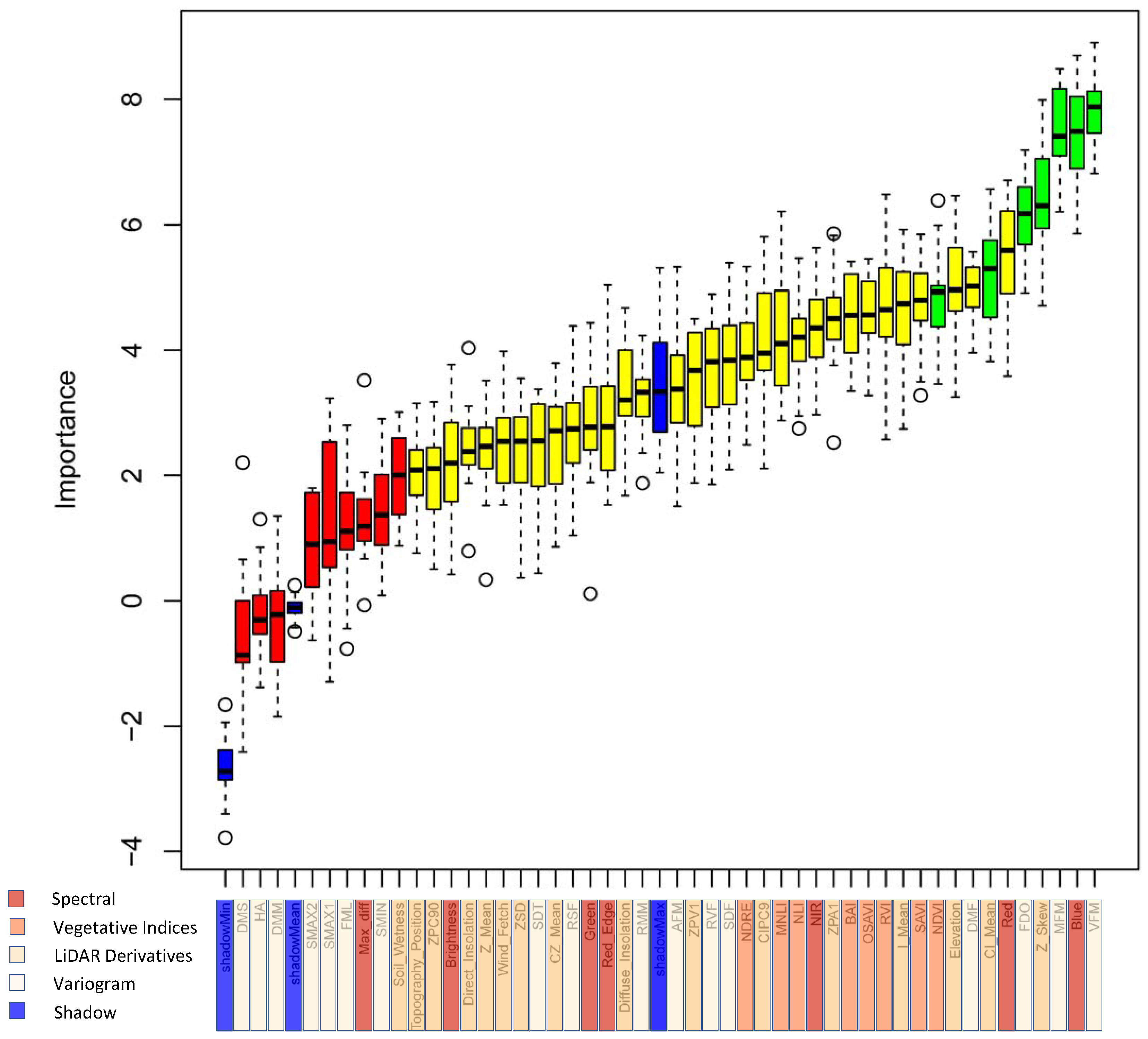
- It evaluates the employment of semivariogram features alongside image-based spectral indices and point-cloud based airborne LiDAR derivatives.
- It presents a methodology for the selection of semantic similarities for semantic characterisation.
2. Background
3. Methodology
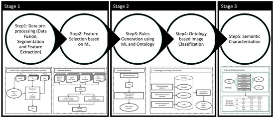
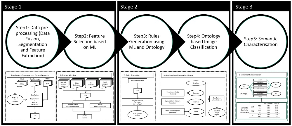
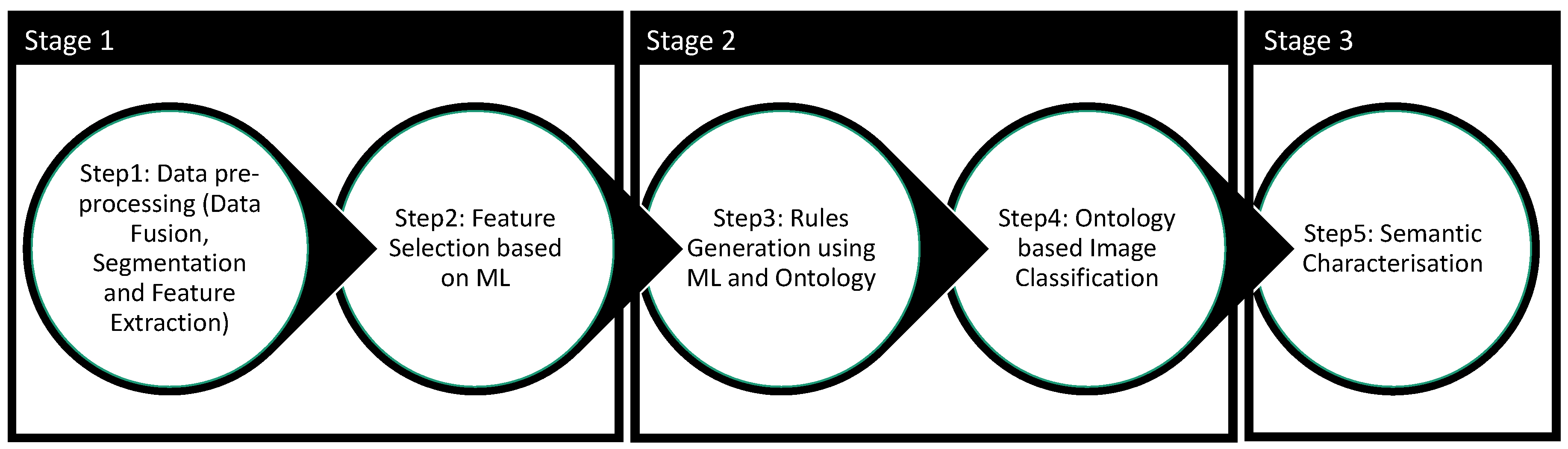
3.1. Extension of an Ontology-Driven Geographic Object-Based Image Analysis (O-GEOBIA) Framework
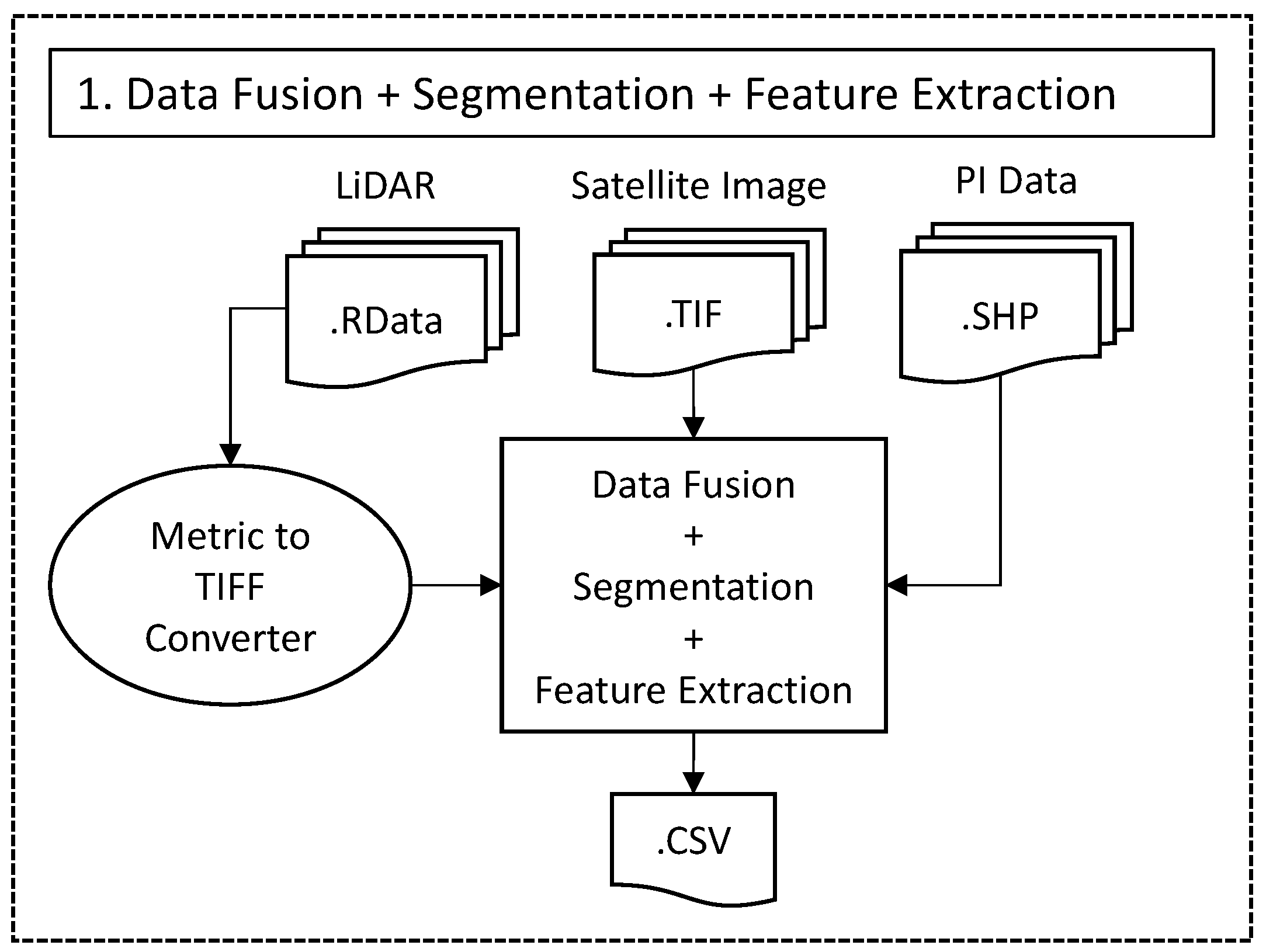
- Step 1
- Data pre-processingThis component comprises a fusion of multi-sensor data, image segmentation and feature extraction. Different multi-sensor data such as satellite imagery and LiDAR are fused, resulting in a new group of features. Image segmentation is carried out to delineate image objects. For each image object, their underlying features value is calculated. Depending on the kind of data used for fusion, different feature variables, such as spectral and spatial, are extracted. The output of this module are extracted feature variables from multi-sensor data, which are input for the next module.
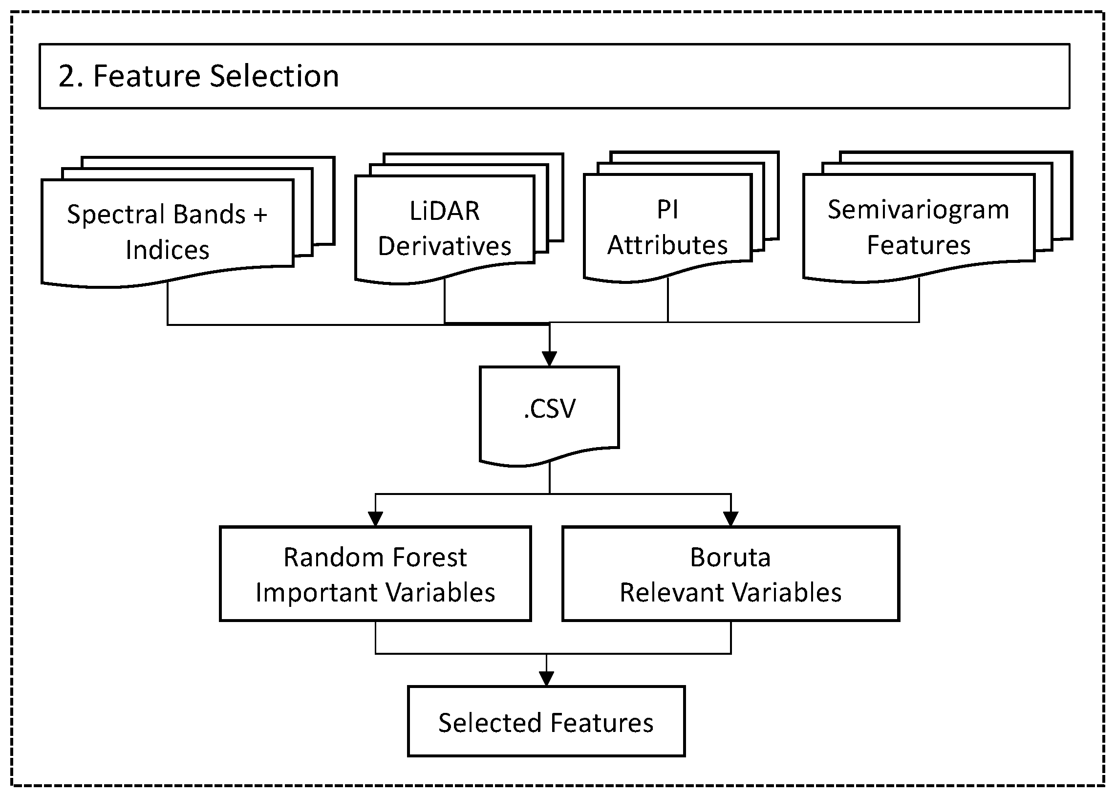
- Step 2
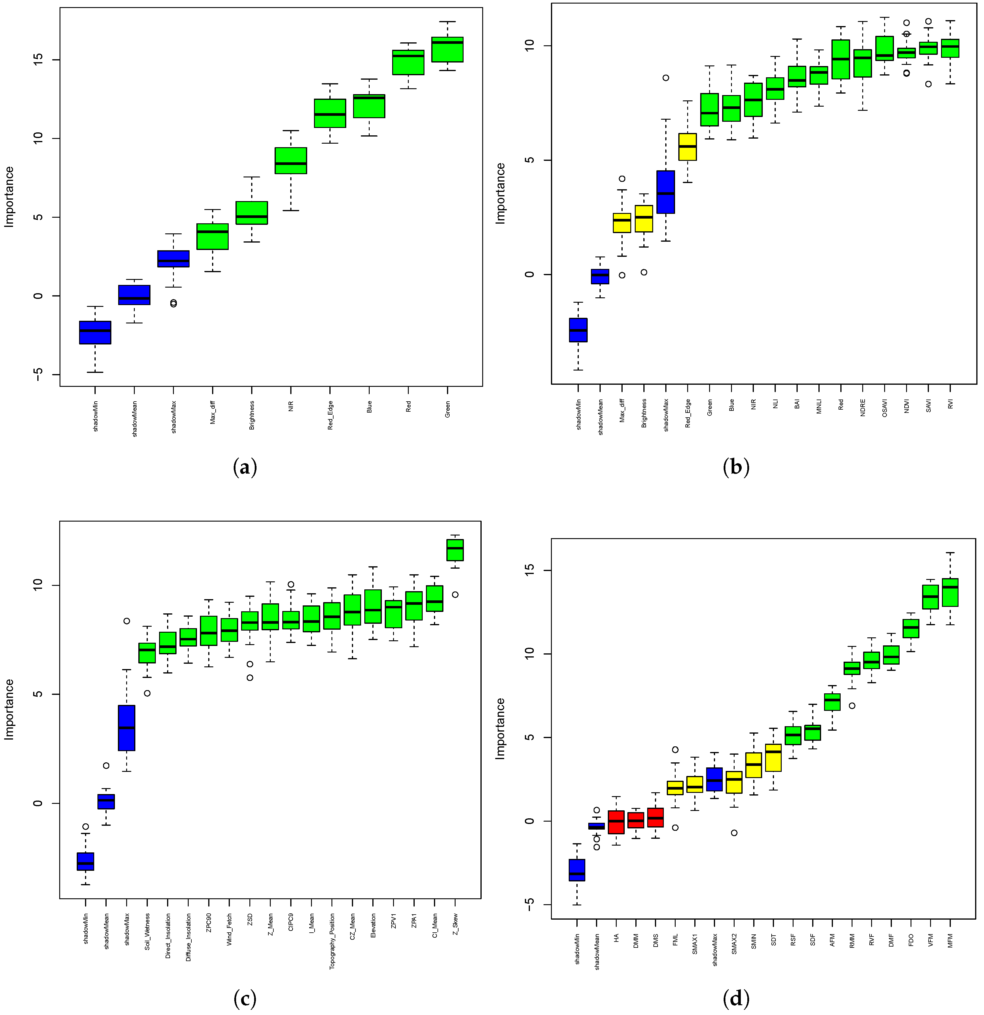
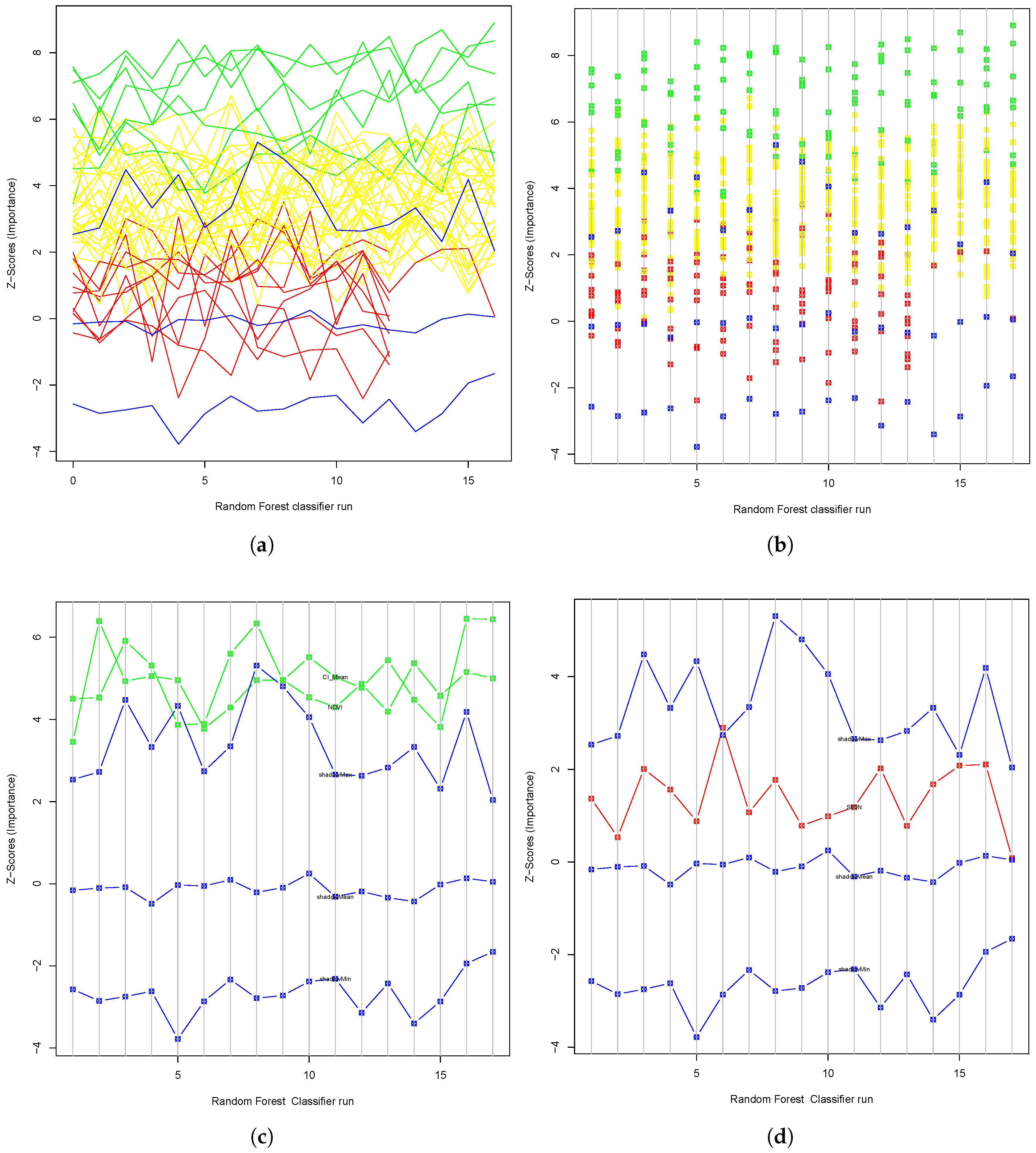
- Feature selection based on MLWith data fusion, a high number of features are available. In this component, we select relevant features using machine learning techniques. To achieve this, we use the Boruta algorithm developed as a wrapper around the Random Forest classifier for identification of important and relevant variables. In this work, we aim to illustrate the importance of feature selection in multi-sensor data with experimental results.
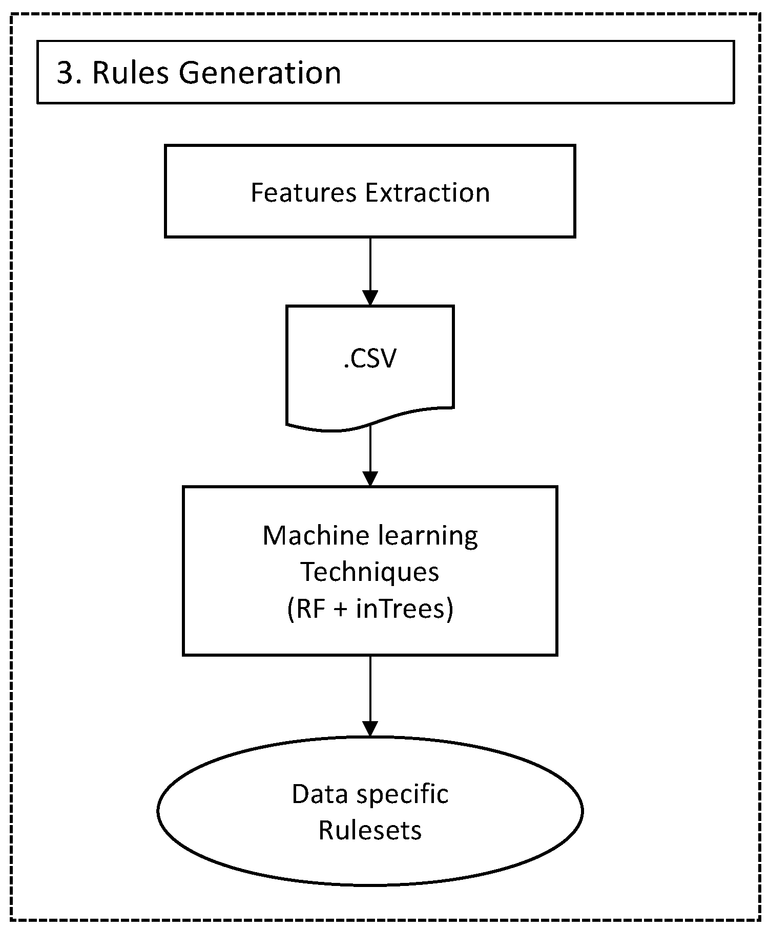
- Step 3
- Rules generation using ML and OntologyAfter selection of features, we use the inTrees (interpretable Trees) framework for automatic extraction of classification rules from the datasets. These rules are added to an ontology along with the expert-defined rules from the next module.
- Step 4
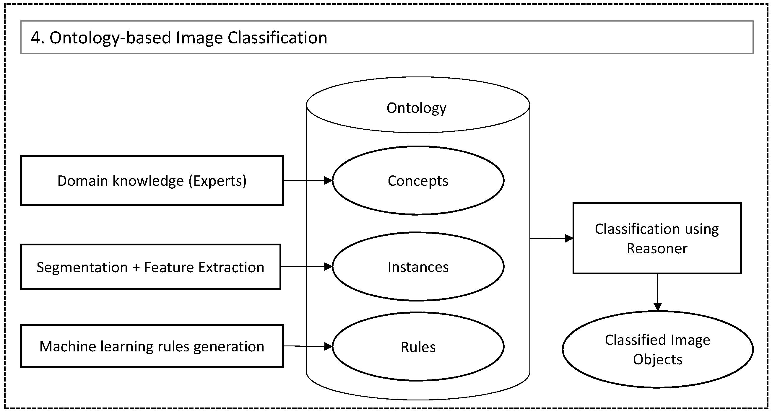
- Ontology based image classificationFor image classification, the ontological framework proposed in [6] is adopted. The classification experiments are based on spectral, LiDAR and variogram based features.
- Step 5
- Semantic characterisationFinally, for semantic characterisation, semantic similarities between the different domain classes, as defined in an ontology, are measured. Based on semantic distances, a semantic variogram is calculated for the characterisation of domain classes. The semantic variogram is used as a metric to characterise the variability between classes based on semantic distances.
3.2. Contextual Experimental Design
- The feature attributes approach helps in the creation of classification rules but ignores spatial relationships. The measurement data used in this approach include spectral and LiDAR data.
- The spatial relationships approach addresses spatial relationships and specifically contributes to the classification using measures of autocorrelation. A variogram is used in this approach.
- The semantic relations approach is based on the semantic relations between classes and uses an ontology. A semantic variogram is used for this approach.
3.2.1. Feature Attributes
3.2.2. Spatial Relations
3.2.3. Semantic Relations
3.2.4. Semantic Similarities
- Hierarchy-basedThe hierarchy-based similarity measure is a distance-based similarity measure that uses the conceptual hierarchy to calculate the distance between concepts. This distance is a count of the number of edges on the path or a count of the number of nodes in the path linking the two concepts. Thus it is also known as the path-based similarity or edge-counting similarity measures [39,55]. The semantic distance is measured by calculating the number of edges or the number of nodes that have to be traversed in a hierarchy from one concept to other. In Wu and Palmer’s hierarchy-based measure [56], the similarity is calculated using the distance from the root to the common subsumer of and using the equation below.In Equation (3), is Wu and Palmer’s [56] hierarchy-based similarity measure, and are the concepts whose semantic similarities are measured, is the common subsumer of and , root is the top concept in the hierarchy, and len(root, ) is the number of nodes on the path from concept to the root concept.
- Information-content-basedInformation content (IC) based similarity measures use a measure of how specific a concept is in a given ontology. If a concept is more specific, there will be high information content and inversely less information content with the more general concept. The ontology-based IC uses the ontology structure itself [57] which is defined in Equation (4) as below.where is the Similarity based on Information Content (IC), is the number of descendants for concept C and is the maximum number of concepts in the ontology.
- Feature-basedIn an ontology, a class can be treated equivalent to another class if both classes have the same number of equivalent attributes. This means that the two classes are more highly similar when more common attributes exist between the classes. Thus the feature-based similarity measure is a degree of class similarity to another class. It is measured using the number of attributes that match between two classes. This approach consists of combining feature-based similarities within an ontology. The Tversky index is used to measure similarity based on the distinct features of class A to B, distinct features of class B to A, and common features of class A and B [58].where, and are the sets of attributes of classes and ; |∩| is the total number of formal attributes shared by and , || and || represent the number of formal attributes of and ; = = 1 which is equivalent to Jaccard index.
4. Experiment: Case Study on Tasmanian Forests
4.1. Tasmanian Forest-Type Mapping
4.2. Assumptions
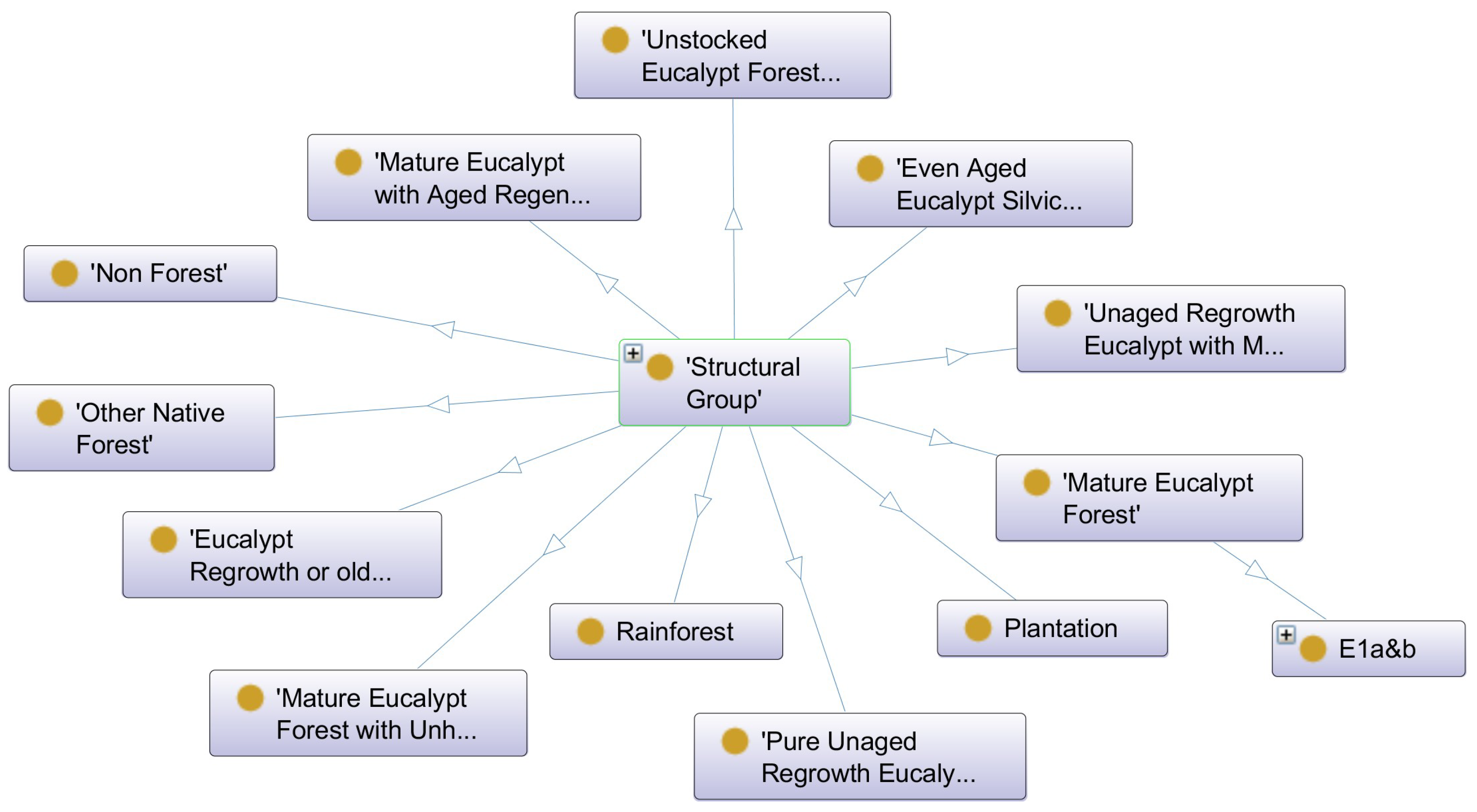
4.3. Ontology for Forest-Type Mapping
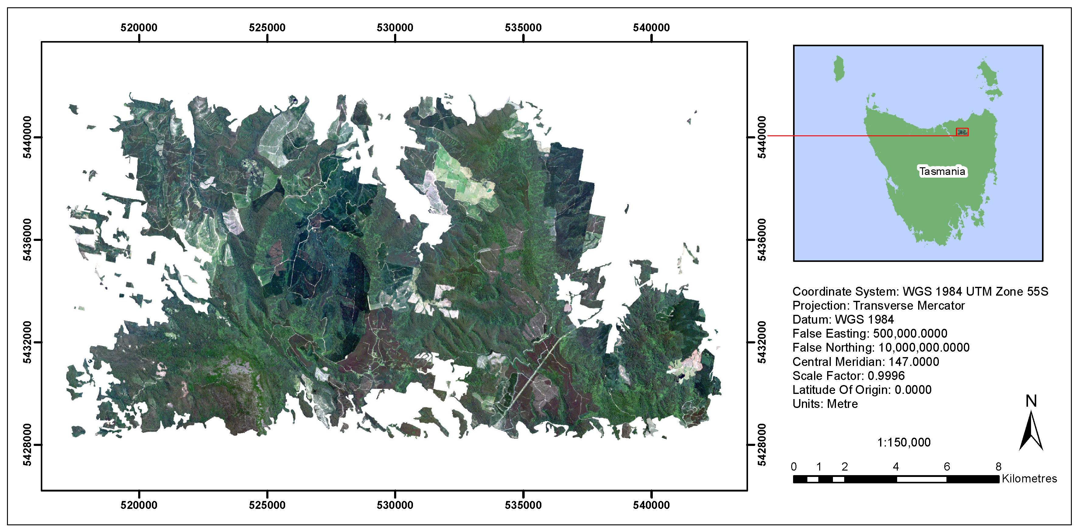
4.4. Study Area
4.5. Data
4.5.1. Satellite Image Data
4.5.2. LiDAR Data
4.5.3. Photo Interpretation (PI) Data
5. Implementation
5.1. Data Fusion, Segmentation and Feature Extraction of Multi-Sensor Data
5.2. Feature Selection
5.3. Rules Generation
5.4. Ontology-Based Image Classification
6. Results
6.1. Feature Selection
6.2. Classification Accuracy Assessment
6.3. Semantic Similarity Assessment
7. Discussion
7.1. Importance of Feature Selection in the Fused Multi-Sensor Data
7.2. Evaluation of Semivariogram Features
7.3. Selection of Semantic Similarities for Multi-Sensor Remote Sensing Data
7.4. Limitations
8. Conclusions
Author Contributions
Funding
Acknowledgments
Conflicts of Interest
Abbreviations
| DEM | Digital Elevation Model |
| DSM | Digital Surface Model |
| FC2011 | Forest Class 2011 |
| GEOBIA | Geographic Object-Based Image Analysis |
| IC | Information Content |
| inTrees | interpretable Trees |
| LAS file | LASer file |
| LiDAR | Light Detection and Ranging |
| MAT | Mature Eucalypt Forest |
| ML | Machine Learning |
| MZSA | Maximum Z Score |
| O-GEOBIA | Ontology-driven Geographic Object-Based Image Analysis |
| OWL | Web Ontology Language |
| PI | Photo Interpretation |
| REG | Pure Unaged Regrowth Eucalypt Forest |
| r2VIM | Recurrent relative variable importance |
| RF | Random Forests |
| SIL | Even Aged Eucalypt Silvicultural Regeneration forest |
| SWRL | Semantic Web Rule Language |
| UTM | Universal Transverse Mercator |
| WGS84 | World Geodetic System 1984 |
References
- Blaschke, T.; Hay, G.J.; Kelly, M.; Lang, S.; Hofmann, P.; Addink, E.; Queiroz Feitosa, R.; van der Meer, F.; van der Werff, H.; van Coillie, F.; et al. Geographic Object-Based Image Analysis - Towards a new paradigm. ISPRS J. Photogramm. Remote Sens. 2014, 87, 180–191. [Google Scholar] [CrossRef] [PubMed]
- Addink, E.A.; Van Coillie, F.M.B.; De Jong, S.M. Introduction to the GEOBIA 2010 special issue: From pixels to geographic objects in remote sensing image analysis. Int. J. Appl. Earth Observ. Geoinf. 2012, 15, 1–6. [Google Scholar] [CrossRef]
- Argyridis, A.; Argialas, D.P. Building change detection through multi-scale GEOBIA approach by integrating deep belief networks with fuzzy ontologies. Int. J. Image Data Fusion 2016, 7, 148–171. [Google Scholar] [CrossRef]
- Arvor, D.; Durieux, L.; Andrés, S.; Laporte, M.A. Advances in Geographic Object-Based Image Analysis with ontologies: A review of main contributions and limitations from a remote sensing perspective. ISPRS J. Photogramm. Remote Sens. 2013, 82, 125–137. [Google Scholar] [CrossRef]
- Rajbhandari, S.; Aryal, J.; Osborn, J.; Lucieer, A.; Musk, R. Employing Ontology to Capture Expert Intelligence within GEOBIA: Automation of the Interpretation Process. In Remote Sensing and Cognition: Human Factors in Image Interpretation; White, R., Coltekin, A., Hoffman, R., Eds.; Book Section 8; CRC Press: Boca Raton, FL, USA, 2018; pp. 151–170. [Google Scholar]
- Rajbhandari, S.; Aryal, J.; Osborn, J.; Musk, R.; Lucieer, A. Benchmarking the Applicability of Ontology in Geographic Object-Based Image Analysis. ISPRS Int. J. Geo-Inf. 2017, 6, 386. [Google Scholar] [CrossRef]
- Schmitt, M.; Zhu, X.X. Data Fusion and Remote Sensing: An ever-growing relationship. IEEE Geosci. Remote Sens. Mag. 2016, 4, 6–23. [Google Scholar] [CrossRef]
- Dong, J.; Zhuang, D.; Huang, Y.; Fu, J. Advances in Multi-Sensor Data Fusion: Algorithms and Applications. Sensors 2009, 9, 7771–7784. [Google Scholar] [CrossRef] [PubMed]
- Lu, M.; Chen, B.; Liao, X.; Yue, T.; Yue, H.; Ren, S.; Li, X.; Nie, Z.; Xu, B. Forest Types Classification Based on Multi-Source Data Fusion. Remote Sens. 2017, 9, 1153. [Google Scholar] [CrossRef]
- Sadjadi, F. Comparative Image Fusion Analysais. In Proceedings of the 2005 IEEE Computer Society Conference on Computer Vision and Pattern Recognition (CVPR’05)—Workshops, San Diego, CA, USA, 21–23 September 2005; p. 8. [Google Scholar]
- Zhang, J. Multi-source remote sensing data fusion: Status and trends. Int. J. Image Data Fusion 2010, 1, 5–24. [Google Scholar] [CrossRef]
- Johansen, K.; Tiede, D.; Blaschke, T.; Arroyo, L.A.; Phinn, S. Automatic Geographic Object Based Mapping of Streambed and Riparian Zone Extent from LiDAR Data in a Temperate Rural Urban Environment, Australia. Remote Sens. 2011, 3, 1139–1156. [Google Scholar] [CrossRef]
- Kempeneers, P.; Sedano, F.; Seebach, L.; Strobl, P.; San-Miguel-Ayanz, J. Data Fusion of Different Spatial Resolution Remote Sensing Images Applied to Forest-Type Mapping. IEEE Trans. Geosci. Remote Sens. 2011, 49, 4977–4986. [Google Scholar] [CrossRef]
- Tönjes, R.; Growe, S.; Bückner, J.; Liedtke, C.E. Knowledge-based interpretation of remote sensing images using semantic nets. Photogramm. Eng. Remote Sens. 1999, 65, 811–821. [Google Scholar]
- Durand, N.; Derivaux, S.; Forestier, G.; Wemmert, C.; Gancarski, P.; Boussaid, O.; Puissant, A. Ontology-based object recognition for remote sensing image interpretation. In Proceedings of the 19th IEEE International Conference on Tools with Artificial Intelligence, Patras, Greece, 29–31 October 2007; pp. 472–479. [Google Scholar]
- Costa, G.; Feitosa, R.; Fonseca, L.; Oliveira, D.; Ferreira, R.; Castejon, E. Knowledge-based interpretation of remote sensing data with the InterIMAGE system: Major characteristics and recent developments. In Proceedings of the 3rd GEOBIA, Ghent, Belgium, 29 June–2 July 2010. [Google Scholar]
- Mundy, J.L.; Dong, Y.; Gilliam, A.; Wagner, R. The Semantic Web and Computer Vision: Old AI Meets New AI. In Proceedings of the Automatic Target Recognition XXVIII, Orlando, FL, USA, 30 April 2018; Volume 10648, p. 8. [Google Scholar]
- Belgiu, M.; Hofer, B.; Hofmann, P. Coupling formalized knowledge bases with object-based image analysis. Remote Sens. Lett. 2014, 5, 530–538. [Google Scholar] [CrossRef]
- Gu, H.; Li, H.; Yan, L.; Liu, Z.; Blaschke, T.; Soergel, U. An Object-Based Semantic Classification Method for High Resolution Remote Sensing Imagery Using Ontology. Remote Sens. 2017, 9, 329. [Google Scholar] [CrossRef]
- Bittner, T.; Winter, S. On Ontology in Image Analysis; Integrated Spatial Databases; Springer: Berlin/Heidelberg, Germany, 2000; pp. 168–191. [Google Scholar]
- Frank, A.U. Tiers of ontology and consistency constraints in geographical information systems. Int. J. Geogr. Inf. Sci. 2001, 15, 667–678. [Google Scholar] [CrossRef]
- Winter, S. Ontology: Buzzword or paradigm shift in GI science? Int. J. Geogr. Inf. Sci. 2001, 15, 587–590. [Google Scholar] [CrossRef]
- Kuhn, W. Ontologies in support of activities in geographical space. Int. J. Geogr. Inf. Sci. 2001, 15, 613–631. [Google Scholar] [CrossRef]
- Agarwal, P. Ontological considerations in GIScience. Int. J. Geogr. Inf. Sci. 2005, 19, 501–536. [Google Scholar] [CrossRef]
- Blaschke, T.; Lang, S.; Lorup, E.; Strobl, J.; Zeil, P. Object-oriented image processing in an integrated GIS/remote sensing environment and perspectives for environmental applications. Environ. Inf. Plan. Politics Public 2000, 2, 555–570. [Google Scholar]
- Mezaris, V.; Kompatsiaris, I.; Strintzis, M.G. An ontology approach to object-based image retrieval. In Proceedings of the 2003 International Conference on Image Processing (Cat. No.03CH37429), Barcelona, Spain, 14–17 September 2003; Volume 2, p. II-511. [Google Scholar]
- Hay, G.J.; Castilla, G. Geographic Object-Based Image Analysis (GEOBIA): A new name for a new discipline. In Object-Based Image Analysis: Spatial Concepts for Knowledge-Driven Remote Sensing Applications; Blaschke, T., Lang, S., Hay, G.J., Eds.; Book Section Chapter 4; Lecture Notes in Geoinformation and Cartography; Springer: Berlin/Heidelberg, Germany, 2008; pp. 75–89. [Google Scholar]
- Andrés, S.; Pierkot, C.; Arvor, D. Towards a Semantic Interpretation of Satellite Images by Using Spatial Relations Defined in Geographic Standards. In Proceedings of the Fifth International Conference on Advanced Geographic Information Systems, Applications, and Services, Nice, France, 24 February–1 March 2013. [Google Scholar]
- Gruber, T.R. A translation approach to portable ontology specifications. Knowl. Acquis. 1993, 5, 199–220. [Google Scholar] [CrossRef]
- Pohl, C.; Van Genderen, J.L. Review article Multisensor image fusion in remote sensing: Concepts, methods and applications. Int. J. Remote Sens. 1998, 19, 823–854. [Google Scholar] [CrossRef]
- Huete, A.R. Vegetation indices, remote sensing and forest monitoring. Geogr. Compass 2012, 6, 513–532. [Google Scholar] [CrossRef]
- Wu, X.; Peng, J.; Shan, J.; Cui, W. Evaluation of semivariogram features for object-based image classification. Geo-Spatial Inf. Sci. 2015, 18, 159–170. [Google Scholar] [CrossRef]
- Kohavi, R.; John, G.H. Wrappers for feature subset selection. Artif. Intell. 1997, 97, 273–324. [Google Scholar] [CrossRef]
- Blum, A.L.; Langley, P. Selection of relevant features and examples in machine learning. Artif. Intell. 1997, 97, 245–271. [Google Scholar] [CrossRef]
- Kursa, M.B.; Rudnicki, W.R. Feature selection with the Boruta package. J. Stat. Softw. 2010. [Google Scholar] [CrossRef]
- Breiman, L. Random Forests. Mach. Learn. 2001, 45, 5–32. [Google Scholar] [CrossRef]
- Langley, P.; Simon, H.A. Applications of machine learning and rule induction. Commun. ACM 1995, 38, 54–64. [Google Scholar] [CrossRef]
- Ben-David, A.; Mandel, J. Classification Accuracy: Machine Learning vs. Explicit Knowledge Acquisition. Mach. Learn. 1995, 18, 109–114. [Google Scholar] [CrossRef]
- Sánchez, D.; Batet, M.; Isern, D.; Valls, A. Ontology-based semantic similarity: A new feature-based approach. Expert Syst. Appl. 2012, 39, 7718–7728. [Google Scholar] [CrossRef]
- Cross, V.; Xueheng, H. Fuzzy set and semantic similarity in ontology alignment. In Proceedings of the 2012 IEEE International Conference on Fuzzy Systems, Brisbane, QLD, Australia, 10–15 June 2012; pp. 1–8. [Google Scholar]
- Pearson, R.L.; Miller, L.D. Remote mapping of standing crop biomass for estimation of the productivity of the shortgrass prairie. In Proceedings of the Eighth International Symposium on Remote Sensing of Environment, Ann Arbor, MI, USA, 2–6 October 1972; p. 1355. [Google Scholar]
- Rouse, J.W., Jr. Monitoring the Vernal Advancement and Retrogradation (Green Wave Effect) of Natural Vegetation; FAO: Rome, Italy, 1973. [Google Scholar]
- Gitelson, A.; Merzlyak, M.N. Spectral Reflectance Changes Associated with Autumn Senescence of Aesculus hippocastanum L. and Acer platanoides L. Leaves. Spectral Features and Relation to Chlorophyll Estimation. J. Plant Physiol. 1994, 143, 286–292. [Google Scholar] [CrossRef]
- Huete, A.R. A soil-adjusted vegetation index (SAVI). Remote Sens. Environ. 1988, 25, 295–309. [Google Scholar] [CrossRef]
- Rondeaux, G.; Steven, M.; Frederic, B. Optimization of Soil-Adjusted Vegetation Indices. Remote Sens. Environ. 1996, 55, 95–107. [Google Scholar] [CrossRef]
- Goel, N.S.; Qin, W. Influences of canopy architecture on relationships between various vegetation indices and LAI and FPAR: A computer simulation. Remote Sens. Rev. 1994, 10, 309–347. [Google Scholar] [CrossRef]
- Yang, Z.J.; Tsubakihara, H.; Kanae, S.; Wada, K.; Su, C.Y. A novel robust nonlinear motion controller with disturbance observer. IEEE Trans. Control Syst. Technol. 2008, 16, 137–147. [Google Scholar] [CrossRef]
- Chuvieco, E.; Martín, M.P.; Palacios, A. Assessment of different spectral indices in the red-near-infrared spectral domain for burned land discrimination. Int. J. Remote Sens. 2002, 23, 5103–5110. [Google Scholar] [CrossRef]
- Balaguer, A.; Ruiz, L.A.; Hermosilla, T.; Recio, J.A. Definition of a comprehensive set of texture semivariogram features and their evaluation for object-oriented image classification. Comput. Geosci. 2010, 36, 231–240. [Google Scholar] [CrossRef]
- Powers, R.P.; Hermosilla, T.; Coops, N.C.; Chen, G. Remote sensing and object-based techniques for mapping fine-scale industrial disturbances. Int. J. Appl. Earth Observ. Geoinf. 2015, 34, 51–57. [Google Scholar] [CrossRef]
- Atkinson, P.M.; Lewis, P. Geostatistical classification for remote sensing: An introduction. Comput. Geosci. 2000, 26, 361–371. [Google Scholar] [CrossRef]
- Ahlqvist, O.; Shortridge, A. Spatial and semantic dimensions of landscape heterogeneity. Landsc. Ecol. 2010, 25, 573–590. [Google Scholar] [CrossRef]
- Ahlqvist, O.; Shortridge, A. Characterizing Land Cover Structure with Semantic Variograms. In Progress in Spatial Data Handling: 12th International Symposium on Spatial Data Handling; Riedl, A., Kainz, W., Elmes, G.A., Eds.; Springer: Berlin/Heidelberg, Germany, 2006; pp. 401–415. [Google Scholar]
- Gan, M.; Dou, X.; Jiang, R. From Ontology to Semantic Similarity: Calculation of Ontology-Based Semantic Similarity. Sci. World J. 2013, 2013, 11. [Google Scholar] [CrossRef] [PubMed]
- Cross, V.; Yu, X.; Hu, X. Unifying ontological similarity measures: A theoretical and empirical investigation. Int. J. Approx. Reason. 2013, 54, 861–875. [Google Scholar] [CrossRef]
- Wu, Z.; Palmer, M. Verbs Semantics and Lexical Selection. In Proceedings of the 32nd Annual Meeting on Association for Computational Linguistics (ACL ’94), Stroudsburg, PA, USA, 27–30 June 1994; pp. 133–138. [Google Scholar]
- Seco, N.; Veale, T.; Hayes, J. An intrinsic information content metric for semantic similarity in WordNet. In Proceedings of the 16th European Conference on Artificial Intelligence, Valencia, Spain, 22–27 August 2004; pp. 1089–1090. [Google Scholar]
- Tversky, A. Features of similarity. Psychol. Rev. 1977, 84, 327–352. [Google Scholar] [CrossRef]
- Stone, M.G. Forest-type mapping by photo-interpretation: A multi-purpose base for Tasmania’s forest management. Tasforests 1998, 10, 1–15. [Google Scholar]
- Ruiz, L.A.; Recio, J.A.; Fernández-Sarría, A.; Hermosilla, T. A feature extraction software tool for agricultural object-based image analysis. Comput. Electron. Agric. 2011, 76, 284–296. [Google Scholar] [CrossRef]
- Nilsson, R.; Peña, J.M.; Björkegren, J.; Tegnér, J. Consistent Feature Selection for Pattern Recognition in Polynomial Time. J. Mach. Learn. Res. 2007, 8, 589–612. [Google Scholar]
- Kursa, M.B.; Rudnicki, W.R. R Package ‘Boruta’. Available online: https://cran.r-project.org/web/packages/Boruta/Boruta.pdf (accessed on 4 August 2018).
- Deng, H. Interpreting Tree Ensembles with inTrees; Springer: Berlin, Germany, 2014. [Google Scholar]
- Horrocks, I.; Patel-Schneider, P.F.; Boley, H.; Tabet, S.; Grosof, B.; Dean, M. SWRL: A semantic web rule language combining OWL and RuleML. W3C Memb. Submiss. 2004, 21, 79. [Google Scholar]
- Motik, B.; Patel-Schneider, P.F.; Parsia, B.; Bock, C.; Fokoue, A.; Haase, P.; Hoekstra, R.; Horrocks, I.; Ruttenberg, A.; Sattler, U. OWL 2 web ontology language: Structural specification and functional-style syntax. W3C Recomm. 2009, 27, 159. [Google Scholar]
- Sirin, E.; Parsia, B.; Grau, B.C.; Kalyanpur, A.; Katz, Y. Pellet: A practical OWL-DL reasoner. Web Semant. Sci. Serv. Agents World Wide Web 2007, 5, 51–53. [Google Scholar] [CrossRef]
- Altmann, A.; Toloşi, L.; Sander, O.; Lengauer, T. Permutation importance: A corrected feature importance measure. Bioinformatics 2010, 26, 1340–1347. [Google Scholar] [CrossRef] [PubMed]
- Szymczak, S.; Holzinger, E.; Dasgupta, A.; Malley, J.D.; Molloy, A.M.; Mills, J.L.; Brody, L.C.; Stambolian, D.; Bailey-Wilson, J.E. r2VIM: A new variable selection method for random forests in genome-wide association studies. BioData Min. 2016, 9, 7. [Google Scholar] [CrossRef] [PubMed]
- Janitza, S.; Celik, E.; Boulesteix, A.L. A computationally fast variable importance test for random forests for high-dimensional data. Adv. Data Anal. Classif. 2016. [Google Scholar] [CrossRef]
- Degenhardt, F.; Seifert, S.; Szymczak, S. Evaluation of variable selection methods for random forests and omics data sets. Brief. Bioinformat. 2017. [Google Scholar] [CrossRef] [PubMed]
- Belgiu, M.; Drăguţ, L. Random forest in remote sensing: A review of applications and future directions. ISPRS J. Photogramm. Remote Sens. 2016, 114, 24–31. [Google Scholar] [CrossRef]
- St-Onge, B.A.; Cavayas, F. Automated forest structure mapping from high resolution imagery based on directional semivariogram estimates. Remote Sens. Environ. 1997, 61, 82–95. [Google Scholar] [CrossRef]
- Yue, A.; Zhang, C.; Yang, J.; Su, W.; Yun, W.; Zhu, D. Texture extraction for object-oriented classification of high spatial resolution remotely sensed images using a semivariogram. Int. J. Remote Sens. 2013, 34, 3736–3759. [Google Scholar] [CrossRef]
- Murray, H.; Lucieer, A.; Williams, R. Texture-based classification of sub-Antarctic vegetation communities on Heard Island. Int. J. Appl. Earth Observ. Geoinf. 2010, 12, 138–149. [Google Scholar] [CrossRef]
- Blaschke, T. Object based image analysis for remote sensing. ISPRS J. Photogramm. Remote Sens. 2010, 65, 2–16. [Google Scholar] [CrossRef]
- Lang, S. Object-based image analysis for remote sensing applications: Modeling reality—Dealing with complexity. In Object-Based Image Analysis: Spatial Concepts for Knowledge-Driven Remote Sensing Applications; Blaschke, T., Lang, S., Hay, G.J., Eds.; Springer: Berlin/Heidelberg, Germany, 2008; pp. 3–27. [Google Scholar]
- Akmal, S.; Shih, L.H.; Batres, R. Ontology-based similarity for product information retrieval. Comput. Ind. 2014, 65, 91–107. [Google Scholar] [CrossRef]
- Snchez, D.; Moreno, A. Learning non-taxonomic relationships from web documents for domain ontology construction. Data Knowl. Eng. 2008, 64, 600–623. [Google Scholar] [CrossRef]
Sample Availability: The codes developed in R language are available upon request to the corresponding author for testing the replicability of this research. |


| Type | Name |
|---|---|
| Spectral | Brightness |
| Blue | |
| Green | |
| NIR | |
| Red | |
| Red Edge | |
| LiDAR | Canopy Height (CH) |
| Height | |
| Canopy Intensity (CI) | |
| Intensity | |
| Elevation | |
| Soil Wetness | |
| Wind Fetch | |
| PI data | FC2011 |
| Name | Equation | Notes | References |
|---|---|---|---|
| RVI | Ratio Vegetation Index | Pearson & Miller (1972) [41] | |
| NDVI | Normalised Difference Vegetative Index | Rouse, J.W., Jr. (1974) [42] | |
| NDRE | Normalised Difference Red Edge Index | Gitelson et al. (1994) [43] | |
| SAVI | Soil Adjusted Vegetation Index | Huete, A.R. (1988) [44] | |
| OSAVI | Optimised Soil Adjusted Vegetation Index | Rondeaux et al. (1996) [45] | |
| NLI | Non Linear Index | Goel & Qin (1994) [46] | |
| MNLI | Modified Non Linear Index | Yang et al. (2008) [47] | |
| BAI | Burn Area Index | Chuvieco et al. (2002) [48] |
| Name | Equation | Notes |
|---|---|---|
| RVF | Ratio between total variance and first semivariance | |
| RSF | Ratio between the first and the second semivariance | |
| FDO | First derivative near the origin | |
| SDT | Second derivative at third lag | |
| FML | First maximum lag value | |
| MFM | Mean of the semivariogram values up to the first maximum | |
| VFM | Variance of the semivariogram values up to the first maximum | |
| DMF | Difference between MFM and the first semivariance | |
| RMM | Ratio between the first local maximum semivariance and MFM | |
| SDF | Second-order difference between first lag and first maximum | |
| AFM | Second-order difference between first lag and first maximum | |
| DMS | Distance between the first and the second local maxima | |
| DMM | Distance between the first local maximum and the first local minimum | |
| HA | Hole area |
| Code | Name | Description |
|---|---|---|
| Y | Young Regeneration | Young native regeneration less than 20 years old. |
| R | Regrowth | Regrowth or regeneration older than 20 years. |
| M | Mature or Senescing | Mature or senescent (over-mature) forest. |
| U | Unknown | Unknown growth stage. |
| N | Not Applicable | Not applicable. |
| Code | Name/Description |
|---|---|
| MAT | Mature Eucalypt Forest, (with neither Regrowth nor aged eucalypt Regeneration) |
| MUR | Mature Eucalypt Forest with Unheighted Regrowth (and without aged eucalypt regeneration) |
| MAR | Mature Eucalypt with Aged Regeneration (from partial logging) |
| RGM | Unaged Regrowth Eucalypt with Mature (and without aged eucalypt regeneration) |
| REG | Pure Unaged Regrowth Eucalypt (and without mature or aged eucalypt regeneration) |
| RGA | Eucalypt Regrowth or older Aged Regeneration, with younger Aged Regeneration (from partial logging) |
| SIL | Even Aged Eucalypt Silvicultural Regeneration (An aged regeneration element, whether heighted or not, with no other mature or unaged eucalypt regrowth or aged eucalypt regeneration present) |
| UST | Unstocked Eucalypt Forest |
| RNF | Rainforest |
| ONF | Other Native Forest |
| PLN | Plantation |
| NOF | Non Forest |
| Bands | Range |
|---|---|
| blue | (0.44–0.51 μm) |
| green | (0.52–0.59 μm) |
| red | (0.63–0.685 μm) |
| red-edge | (0.69–0.73 μm) |
| near-infra-red | (0.76–0.85 μm) |
| Class | Spectral | Spectral + Indices | LiDAR | Variogram | All | ||||||||||
|---|---|---|---|---|---|---|---|---|---|---|---|---|---|---|---|
| M | R | S | M | R | S | M | R | S | M | R | S | M | R | S | |
| M (MAT) | 3 | 4 | 0 | 4 | 3 | 0 | 6 | 9 | 0 | 2 | 3 | 0 | 6 | 2 | 0 |
| R (REG) | 20 | 81 | 1 | 19 | 82 | 1 | 17 | 74 | 1 | 21 | 82 | 1 | 17 | 83 | 1 |
| S (SIL) | 0 | 0 | 0 | 0 | 0 | 0 | 0 | 2 | 0 | 0 | 0 | 0 | 0 | 0 | 0 |
| OA | 77.06% | 78.90% | 73.39% | 77.06% | 81.65% | ||||||||||
| Class | All Available Variables | Relevant Variables | ||||
|---|---|---|---|---|---|---|
| M | R | S | M | R | S | |
| M (MAT) | 6 | 2 | 0 | 8 | 3 | 0 |
| R (REG) | 17 | 83 | 1 | 15 | 82 | 1 |
| S (SIL) | 0 | 0 | 0 | 0 | 0 | 0 |
| OA | 81.65% | 82.57% | ||||
| Wu & Palmer | Tversky | ||
|---|---|---|---|
| MAT | REG | 0.25 | 0.72 |
| SIL | 0.25 | 0.17 | |
| REG | MAT | 0.25 | 0.72 |
| SIL | 0.25 | 0.17 | |
| SIL | MAT | 0.25 | 0.17 |
| REG | 0.25 | 0.17 |
© 2019 by the authors. Licensee MDPI, Basel, Switzerland. This article is an open access article distributed under the terms and conditions of the Creative Commons Attribution (CC BY) license (http://creativecommons.org/licenses/by/4.0/).
Share and Cite
Rajbhandari, S.; Aryal, J.; Osborn, J.; Lucieer, A.; Musk, R. Leveraging Machine Learning to Extend Ontology-Driven Geographic Object-Based Image Analysis (O-GEOBIA): A Case Study in Forest-Type Mapping. Remote Sens. 2019, 11, 503. https://doi.org/10.3390/rs11050503
Rajbhandari S, Aryal J, Osborn J, Lucieer A, Musk R. Leveraging Machine Learning to Extend Ontology-Driven Geographic Object-Based Image Analysis (O-GEOBIA): A Case Study in Forest-Type Mapping. Remote Sensing. 2019; 11(5):503. https://doi.org/10.3390/rs11050503
Chicago/Turabian StyleRajbhandari, Sachit, Jagannath Aryal, Jon Osborn, Arko Lucieer, and Robert Musk. 2019. "Leveraging Machine Learning to Extend Ontology-Driven Geographic Object-Based Image Analysis (O-GEOBIA): A Case Study in Forest-Type Mapping" Remote Sensing 11, no. 5: 503. https://doi.org/10.3390/rs11050503
APA StyleRajbhandari, S., Aryal, J., Osborn, J., Lucieer, A., & Musk, R. (2019). Leveraging Machine Learning to Extend Ontology-Driven Geographic Object-Based Image Analysis (O-GEOBIA): A Case Study in Forest-Type Mapping. Remote Sensing, 11(5), 503. https://doi.org/10.3390/rs11050503