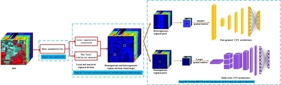
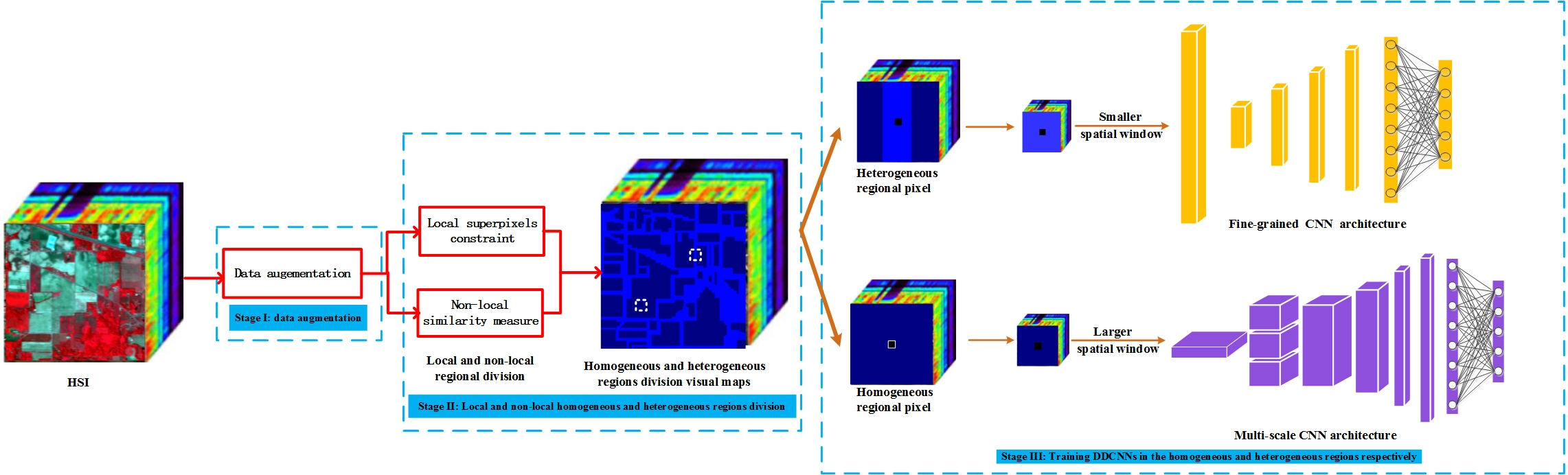
Article

Divide-and-Conquer Dual-Architecture Convolutional Neural Network for Classification of Hyperspectral Images

Key Laboratory of Intelligent Perception and Image Understanding of Ministry of Education, Xidian University, Xi’an 710071, China
*
Author to whom correspondence should be addressed.
Remote Sens. 2019, 11(5), 484; https://doi.org/10.3390/rs11050484
Submission received: 25 January 2019 / Revised: 19 February 2019 / Accepted: 22 February 2019 / Published: 27 February 2019
(This article belongs to the Special Issue Robust Multispectral/Hyperspectral Image Analysis and Classification)

Abstract

:
Convolutional neural network (CNN) is well-known for its powerful capability on image classification. In hyperspectral images (HSIs), fixed-size spatial window is generally used as the input of CNN for pixel-wise classification. However, single fixed-size spatial architecture hinders the excellent performance of CNN due to the neglect of various land-cover distributions in HSIs. Moreover, insufficient samples in HSIs may cause the overfitting problem. To address these problems, a novel divide-and-conquer dual-architecture CNN (DDCNN) method is proposed for HSI classification. In DDCNN, a novel regional division strategy based on local and non-local decisions is devised to distinguish homogeneous and heterogeneous regions. Then, for homogeneous regions, a multi-scale CNN architecture with larger spatial window inputs is constructed to learn joint spectral-spatial features. For heterogeneous regions, a fine-grained CNN architecture with smaller spatial window inputs is constructed to learn hierarchical spectral features. Moreover, to alleviate the problem of insufficient training samples, unlabeled samples with high confidences are pre-labeled under adaptively spatial constraint. Experimental results on HSIs demonstrate that the proposed method provides encouraging classification performance, especially region uniformity and edge preservation with limited training samples.

Graphical Abstract

1. Introduction

With the rapid development of hyperspectral sensors, hyperspectral remote sensing images have become more available. Hyperspectral images (HSIs) often contain hundreds of narrow and contiguous spectral bands in the same scene, with wavelengths spanning the visible to infrared spectrum [1]. The detailed spectral information provided by hyperspectral sensors improves the capacity to differentiate the interesting land-cover classes. It makes HSI classification one of the most promising techniques in many practical applications, including agriculture [2], military [3], astronomy [4], mineralogy [5], surveillance [6], and environmental sciences [7,8].
HSI classification involves two key aspects: feature extraction and classification. Feature extraction is crucial in addressing the “Hughes phenomenon” [9] caused by high-dimensional spectral bands of HSIs. In the early stage of HSI feature extraction, various spectral-based methods were proposed, such as principal component analysis (PCA) [10,11], independent component analysis (ICA) [12,13], manifold learning [14], sparse graph learning [15], and local Fisher's discriminant analysis (LFDA) [16]. These methods are implemented by transforming original high-dimensional data into an appropriate low-dimensional space. However, it is difficult to precisely distinguish different land-cover classes only by spectral information. To address this issue, some researchers make use of spatial information to extract features, such as Gabor filters [17], wavelets [18,19], extended morphological profiles [20], morphological attribute profiles [21], and extended multi-attribute profiles (EMAPs) [22]. Besides, multitask learning has powerful feature extraction ability due to its ability to incorporate shared information across multiple tasks. In one study [23], the kernel low-rank multitask method is proposed to capture multiple features from the 2-D variational mode decomposition domain for multi-/hyperspectral image classification.
A series of representative machine learning-based classification methods are used as classifiers, including k- nearest neighbors [24], logistic regression (LR) [25], extreme learning machine [26], sparse representation-based classification [27,28,29], support vector machine (SVM) [30,31], etc. Among these methods, SVM maximizes the margin among different classes in a kernel-induced feature space. It achieves outstanding performance for HSI classification, especially with small-sized training set.
The mentioned-above methods complete feature extraction and classification individually. Besides, these methods adopt manually-extracted features, which involve massive effort in feature engineering. In 2006, Geoffery Hinton proposed deep learning [32], and deep learning obtained a great success in computer vision [33,34,35,36,37]. Compared with traditional methods, deep learning-based methods extract hierarchical features and train the classifier simultaneously. Moreover, these deep learning-based methods adopt two or more hidden layers to extract more abstract and invariant features of data automatically.
A series of deep learning-based models have been introduced into the classification of HSIs. In one study [38], the stacked autoencoder (SAE) was proposed to extract deep features from hierarchical architecture. Subsequently, sparse SAE [39], denoising SAE [40], and Laplacian SAE [41] were successively proposed. In another study [42], Chen et al. presented a deep belief network (DBN) by learning the restricted Boltzmann machine network layer-by-layer. However, these methods cannot make full use of spatial information, since flattening training samples destroys the spatial structure in HSIs. Besides, there are so many parameters produced by full connection (FC) in these networks that a large number of available training samples are required.
Compared with SAE and DBN, convolutional neural network (CNN) [33] exploits local connections to effectively extract the spatial feature representation and shared weights to significantly decrease the number of parameters. Inspired by these properties, a series of CNN methods [43,44,45,46,47,48,49,50,51,52,53,54] have emerged for HSI classification. Hu et al. proposed a 1-dimensional (1D) CNN-based method to learn hierarchical spectral features of HSIs [50]. Makantasis et al. combined randomized PCA and CNN to encode spatial information of HSIs [51]. However, these two methods only exploit spectral information or spatial information, respectively. Later, some joint spectral-spatial CNN-based methods were proposed [48,51,52]. A dual-channel CNN (DCNN) was constructed to extract spectral and spatial features by 1D-CNN and 2D-CNN separately, then extracted spectral and spatial features were concatenated together [51]. Chen et al. presented another type of joint spatial-spectral feature extraction, where a 3-dimensional (3D) CNN (3DCNN) model was adopted to extract spectral and spatial information simultaneously [52]. However, the performance of these CNN methods depends on the quantity of training samples greatly. Generally, the collection of training samples is difficult in HSIs. Recently, Li et al. proposed a pixel-pair CNN (PPF-CNN) method by reorganizing and relabeling existing training samples [53]. Besides, in several studies [55,56,57], tensor-based models significantly reduced the number of weight parameters required to train the model via tensor decomposition. When the number of training data is limited, tensor-based classification models can perform well. Makantasis et al. proposed tensor-based linear and nonlinear models for HSI classification [55]. The data from all the sensors was fused into a tensor, and damage-sensitive features were extracted for classification in tensor-based models [56]. Recently, some other deep learning models are introduced for HIS [58,59]. A new fully CNN was proposed to extract the deep features of HSIs. Then, the optimized extreme learning machine is used for classification [58].
All the mentioned CNN-based methods [43,44,45,46,47,48,49,50,51,52,53,54] adopt a single fixed network structure for HSI classification. The single network structure ignores the complex land-cover distributions of HSIs. In heterogeneous regions, a large-sized spatial window input covers some samples coming from different classes. These neighbor samples with different classes may lead to misclassification of samples located around the boundaries. In this case, spectral information is mainly required for heterogeneous regions. On the contrary, in homogeneous regions, neighbor samples have similar spectral signatures. A small spatial window input may lack enough contextual information for classification. In this case, spatial and spectral information are required to analyze homogeneous regions simultaneously. Therefore, single fixed network structure may hinder the excellent performance of CNNs for HSI pixel-wise classification.
To address this problem, a novel divide-and-conquer dual-architecture CNN (DDCNN) method is designed for HSI classification. In DDCNN, a new regional division strategy based on local and non-local decisions is devised to divide HSIs into homogeneous and heterogeneous regions, respectively. The non-local decision is performed to search the superpixel-pair similarity in the whole image, while the local decision is made by spatially adjacent samples in the superpixels. For the homogeneous regions, larger-sized spatial windows are selected to extract adequately contextual information. A multi-scale CNN architecture with larger spatial windows is constructed to learn joint spectral-spatial features. For the heterogeneous regions, smaller spatial windows are selected to guarantee the samples belonging to the same class. A fine-gained CNN architecture with smaller spatial windows is constructed to learn hierarchical spectral features. Then, to alleviate the problem of insufficient training samples, unlabeled samples are selected by measuring the spectral similarity under adaptively spatial constraint. The samples with high confidences on the spectral similarity are pre-labeled to expand the training set.
The main contributions of this paper can be summarized as follows. (1) A novel dual-architecture CNN is designed instead of traditional single architecture considering various land-cover distributions of HSIs. In DDCNN, a multi-scale CNN architecture is constructed to improve the uniformity of homogeneous regions, and a fine-grained CNN architecture is constructed to avoid edge over-smoothness. (2) Regional division method-based local and non-local decisions are designed to divide the homogeneous and heterogeneous regions effectively, where superpixel-to-superpixel similarity is utilized in the non-local searching. (3) DDCNN devises a new sample augmentation method based on spectral similarity under adaptively spatial constraints, which alleviates the over-fitting problem of CNNs caused by the imbalance between insufficient training samples and numerous parameters.
The rest of this paper is organized as follows. Section 2 reviews the CNN briefly. Section 3 describes the procedure of the proposed DDCNN method in detail. Then, the experimental validation and corresponding analysis on several hyperspectral datasets are discussed in Section 4. Finally, some concluding remarks and suggestions are provided for further work in Section 5.

2. The Review of Convolutional Neural Networks

CNN, one of the deep leaning models, gains outstanding performance in computer vision tasks, such as classification, detection, and recognition. The architecture of CNN is based on the inspirations from neuroscience [60]. In the biological visual system, the cells in the cortex are sensitive to small regions, known as receptive fields. The strong capability of cells within receptive fields is used to exploit the local spatial correlation in images.
In contrast to other deep learning models, CNN possesses three core ideas: local connections, shared weights, and pooling. Local connections can extract local spatial features effectively corresponding to the receptive fields. Shared weight—that is, the connections between neurons—are replicated across the entire layer, which can significantly reduce the parameters of deep networks. Pooling is also known as downsampling, which extracts more robust features in the translation and deformation.
A traditional CNN is constructed by stacking several convolutional layers, pooling layers, and full connection layers to form deep architecture, where the output of each layer is provided as the input of the next layer. In the convolutional layer, the value of a neuron v i j x y at position ( x , y ) of the j th feature map in the i th layer is denoted as follows:
v i j x y = g ( b i j + m p = 0 P i 1 q = 0 Q i 1 w i j m p q v ( i 1 ) m ( x + p ) ( y + q ) )
g ( x ) = R e L u ( x ) = max ( x , 0 )
where m indexes the feature map in the i 1 th layer connected to the current feature map, w i j m p q is the weights of position ( p , q ) connected to the m th feature map, P i and Q i are the height and width of the spatial window, and b i j is the bias of the j th feature map in the j th layer.

3. Divide-and-Conquer Dual-Architecture CNN(DDCNN)

The flowchart of the proposed DDCNN method is shown in Figure 1. As shown in Figure 1, DDCNN consists of three stages: regional division with local and non-local decisions, dual-architecture CNN-based classification, and data augmentation based on spectral similarity under adaptively spatial constraint. A HSI dataset contains M training samples X t r a i n = { x 1 , , x m , , x M } in an d × 1 feature space, where d is the number of spectral bands, and 1 m M . The class label of training samples is represented by Y = { y 1 , , y m , , y M } ; y m { 1 , , k , , K } , where K is the number of classes, and 1 k K . At the regional division stage, the HSIs are divided into homogeneous and heterogeneous regions by using local and non-local decisions. Then, for the homogeneous regions, a multi-scale CNN architecture with larger-sized spatial window inputs is constructed to learn joint spectral-spatial features. For the heterogeneous regions, a fine-grained CNN architecture with smaller-sized inputs is constructed to learn hierarchical spectral features. Moreover, unlabeled samples with high confidences are selected to expand the training set by measuring the spectral similarity under the adaptive spatial constraint.

3.1. Superpixel Segmentation Based on Entropy Rate

In the superpixel segmentation, the images are divided into many superpixels. Each of them consists of spatially adjacent pixels with similar texture, color, brightness, or other characteristics [61]. Compared with pixel-based methods, superpixel-based methods utilize the spatial structure of the images and show good regional uniformity.
In this paper, the entropy rate method [62] is adopted to generate a 2-D superpixel map in HSIs. Compared with other superpixel segmentation methods, the entropy rate method is a graph-based clustering algorithm. It favors compact and homogenous nonoverlapping clusters, and has a fast computation speed approximated as O ( | V | log | V | ) , where V is the number of superpixels. More details of the entropy rate algorithm can be found in [62]. As shown in Figure 2, the first principal component of HSIs extracted by PCA is utilized as the base image for the superpixel segmentation. Then the base image is divided into V superpixels with adaptive sizes and shapes, denoted as { π 1 , π 2 , , π V } . Each π v   ( 1 v V ) represents the v th superpixels. The segmentation result will be utilized in the regional division and data augmentation methods.

3.2. Regional Division with Local and Non-local Decisions

Most of CNN-based HSI classifications [43,44,45,46,47,48,50,51,52] are designed to exploit the spatial correlation in the neighborhood around the central pixel. That is, hyperspectral neighboring pixels in a spatial window are jointly represented by the CNN model for feature extraction. These CNN models commonly adopt a fixed-size spatial window as the input for feature extraction (e.g., 5 × 5, 27 × 27, etc.). This type of input hinders the excellent performance of CNNs for HSI classification. A large-sized spatial window input may include between-class samples in the heterogeneous regions, and a small-sized input may lead to extracting insufficient contextual information in the homogeneous regions.
Figure 3 illustrates an example for these two situations. In Figure 3, i and j are two samples in the HSIs. These two samples locate in the homogeneous and heterogeneous regions, respectively. Both them belong to the “GREEN” class. For the sample i, a larger spatial window (i.e., black box) contains some samples belonging to “BLUE”, “PURPLE”, and “YELLOW” classes instead of “GREEN” class. In this case, the sample i may be easily misclassified as the “BLUE”, “PURPLE”, or “YELLOW” class. If a smaller spatial window (i.e., red box) is selected, all the samples in the window belong to the “GREEN” class. For the sample j, all the samples in both larger and smaller spatial windows (i.e., black and red boxes) belong to the “GREEN” class. In the case, a larger spatial widow contains more adequately contextual information for feature extraction.
To deal with these two situations, novel regional division method-based local and non-local decisions are designed to divide the HSIs into homogeneous and heterogeneous regions, where different CNN architectures are designed for homogeneous and heterogeneous regions, respectively. The divide and conquer strategy with homogeneous and heterogeneous regions is inspired by a visual attention-based model. Doulamis et al. proposed a fuzzy representation of video content [63]. The divide and conquer concept was first proposed in the multiresolution recursive shortest spanning tree algorithm for video summarization and content-based retrieval [63]. Then, a neural network based scheme was used to select adaptive regions of interest (ROI) [64]. Then, a ROI-based motion-compensated discrete consine transform coder was proposed to extract foreground objects from background in videophones. Derived from the pioneering work on ROI [64], a neurobiological model of visual attention was proposed for video compression [65]. Later, visual attention based model was introduced into hyperspectral image processing [66,67].
(1) Regional Division with Local Decision: In the local decision, entropy rate-based superpixel segmentation is used to generate some homogeneous superpixels. Similar to the masking of edge detection, we choose a square frame (e.g., 3 × 3, 5 × 5) as the filter. If all the samples in the filter are within the same superpixel, the central sample is judged to be in the homogeneous regions. If these samples are divided into multiple superpixels, the central sample is located in the heterogeneous regions of the superpixel segmentation map. Actually, since the superpixel segmentation over-segments the HSIs, the central sample may be uncertain in the ground truth. It may belong to either the homogeneous or heterogeneous region.
Figure 4 illustrates the local regional division based on superpixel segmentation. Take the Indian Pines HSI as an example. Figure 4a shows the ground truth of the Indian Pines HSI. Figure 4b shows the results of entropy rate-based superpixel segmentation on the Indian Pines HSI. The samples i, j, and k represent the central samples located in the different regions. Figure 4c–e corresponds to the filters of the samples i, j, and k. In Figure 4d, since all neighbor samples in the filter belong to the same superpixel, the central sample i is judged to be in the homogeneous regions. In Figure 4c,e, the neighbor samples of the central samples j and k in the filters come from different superpixels. In the superpixel-based local decision, both sample j and k are judged to be in the heterogeneous regions. Actually, the sample k is located at the boundary area of superpixel segmentation map in Figure 4b rather than that of ground truth in Figure 4a. This is the “false boundary” phenomenon caused by the superpixel segmentation map. In the superpixel segmentation map, the samples belonging to the same class may be divided into several superpixels.
Let x i be a central sample and N i be the filter of x i . If all the neighbor samples belong to the same superpixel π v , the central sample x i is judged to be in the homogeneous regions, and vice versa. The regional division based on local decision is formulated as follows:
x i { X H o   if   N i π v ( x i ) X H e   else
where π v ( x i ) denotes the superpixel that the sample x i belongs to. X H o represents the sample set in the homogeneous regions, and X H e represents the sample set in the heterogeneous regions of superpixel segmentation map.
(2) Regional Division with Non-Local Decision: To alleviate the misdivision caused by the false boundary, a novel regional division based on non-local decisions is devised. In the HSIs, local information is used on the assumption that the samples in a local region belong to the same class. However, non-local information is also vital for HSI classification [68,69], since the samples belonging to the same class may be located in different regions.
In the non-local decision, pixel-similarity is extended to superpixel-similarity, which considers the structural information of current samples. For the samples judged in the heterogeneous regions by local decisions, the similarities of the neighbor samples and the current sample are calculated, where the current sample is represented by the samples with the same class in the global searching. Then, the similarities are compared with a calculated adaptive threshold. If the similarities of all the neighbors are larger than the threshold, the current sample is judged to be in the homogeneous region, and vice versa.
Let x i represent a sample judged in heterogeneous regions by local decision, denoted as x i X H e . The filter N i corresponding to x i is divided into L i small patches N i = l = 1 L i N i l . The similarities of the neighbor samples and the current sample are calculated by superpixel-to-superpixel similarity S S ( π v ( x i ) , π v ( N i l ) ) . π v ( N i l ) , which represents the superpixel π v containing the sample set N i l . If all the similarities are larger than the threshold T k of the k th category, the sample x i is judged to be in the homogeneous regions, and vice versa. T k is a set as the minimum superpixel-based similarity of the samples in the k th category. If x i is the unlabeled sample, k is set as the label of the training samples with most similarity. The regional division with non-local decisions is defined as follows:
x i {   X H o   if   S S ( π v ( x i ) , π v ( N i l ) ) T k , 1 i l L i X H e   else T k = min { S S ( π v ( x i ) , π v ( x j ) ) | x i , x j ψ k }
where x j is the sample in the k th category, and π v ( x j ) represents the superpixel correspond the sample x j ; ψ k is the set of training samples in the k th category.
To measure the similarity of two superpixels, the average pooling strategy is applied to exploit the most significant information of superpixels. The similarity of two superpixels is calculated as:
S S ( π v ( x p ) , π v ( x q ) ) = S ( 1 | π v | x p π v x p , 1 | π v | x q π v x q )
where π v ( x p ) and π v ( x q ) represent two different superpixels corresponding to the samples x p an x q , respectively. The similarity measure is calculated by the heat kernel S ( x , x ) = exp ( x x 2 δ 2 ) .
Combining the local and global decisions (3) and (4), the sample is divided into homogeneous and heterogeneous regions according to (6):
x i { X H o   if   N i π v ( x i )   or   S S ( π v ( x i ) , π v ( N i l ) ) T k X H e   else T k = min { S S ( π v ( x i ) , π v ( x j ) ) | x i , x j ψ k }
where X H e is the set of samples in the heterogeneous regions.

3.3. Multi-Scale CNN Architecture

In the HSIs, the spectral signatures of samples in the same class may be different due to varied imaging conditions, e.g., changes in illumination, various environments, different atmospheric conditions, and temporal conditions. Therefore, spatial contexture information is critical for HSI classification. For the samples in the homogenous regions, a multi-scale CNN architecture with larger-sized spatial window inputs is constructed to extract joint spatial and spectral features. The multi-scale convolution consists of 1 × 1, 3 × 3, and 5 × 5 convolutional filters, where a 1 × 1 convolutional filter is used to extract spectral features, while 3 × 3 and 5 × 5 filters are utilized to extract various spatial contextual features.
In the multi-scale CNN architecture, a multi-scale convolutional filter is inspired by the Inception module [35]. The Inception module is used to exploit diverse local spatial structures of the input image, which enables the network to get deeper and wider and achieves state-of-the-art performance in image classification. The effectiveness of the inception module has been demonstrated in the large scale visual recognition challenge (LSVRC) 2014 [35]. The multi-scale convolutional filter is used to extract joint spectral-spatial features for HSI classification in this paper.
The architecture of multi-scale CNN network is shown in Figure 5. The input of multi-scale CNN architecture is larger-sized spatial windows with several principle components of PCA. A multi-scale filter is used in the first convolutional layer to jointly extract spatial structure and spectral correlation. Three feature maps are employed to perform cascade connection to form a joint spectral-spatial feature map. Subsequently, three convolutional layers are stacked one by one to extract hierarchical abstract features of HSIs. Then the extracted feature maps are flattened to a one-dimensional vector used as the input to two full connection layers. Finally, the extracted features are fed into the last soft-max classification layer.
In this model, some regularization methods, data augmentation, dropout, early stop, and batch normalization (BN) are introduced to alleviate the over-fitting problem of CNNs. A new sample augmentation method is devised by pre-labeling the unlabeled samples based on spectral similarity under adaptive spatial constraint. Dropout is used in the second and third convolutional layers by preventing complex co-adaptations. It is used as the regularization technique to relieve the over-fitting problem. Early stop relieves the over-fitting problem by limiting the number of iterations. In addition, batch normalization is used in all the convolutional layers to accelerate the training of networks and reduce the internal covariate shift [70].

3.4. Fine-Grained CNN Architecture

For the samples in the heterogeneous regions, the spatial information is hard to use due to the distribution of different land-cover classes. The distinction for these samples mainly depends on hundreds of contiguous and narrow spectral bands. For these samples, a fine-grained CNN architecture with smaller-sized spatial window inputs is constructed to extract spectral information, where 1 × 1 convolution is used in all the convolutional layers.
The architecture of the fine-grained CNN network is shown in Figure 6. In the fine-grained CNN network, all the spectral bands are retained. The input of fine-grained CNN architecture is smaller-sized spatial windows with all the spectral bands. The 1 × 1 convolution is used in all the four convolutional layers. The 1 × 1 convolutional filter is proposed in Network In Network (NIN) [71], which allows complex and learnable interactions of cross channel information. Furthermore, it is also used to adjust the dimensionality of the feature maps. Here, 1 × 1 convolution is used to learn spectral correlations in the proposed network. Two full connection layers are stacked one by one after the convolutional layers. Finally, the extracted spectral features are fed into the soft-max classification layer. Similar to multi-scale CNN architecture, BN and dropout are used in the same position.

3.5. Data Augmentation Based on Spectral Similarity under the Adaptively Spatial Constraint

Deep learning models depend on a large quantity of training data due to the models being heavily parameterized. However, only limited training samples are available in HSI data. The CNN model tends to be over-fitting for HSI classification. To conquer this issue, a novel data augmentation method based on spectral similarity under adaptive spatial constraint is devised.
In the data augmentation method, superpixels with adaptive sizes and shapes are used for the spatial constraint. In the spatial constraint, unlabeled samples located in the same superpixel with training samples are considered as candidates. Then, unlabeled candidate samples with high confidence, which have the most spectral similarity with training samples, are selected. Finally, these selected unlabeled samples are pre-labeled as the same class with training samples, which are used to expand the training set.
Specifically, x u denotes a current unlabeled sample, and π v ( x u ) represents the superpixel where the sample x u is located. For all the training samples { x m | x m π v } in the superpixel π v , the similarities of current unlabeled sample x u and all the training samples { x m | x m π i } are calculated. Then, the similarities are compared with a calculated threshold T π v , which is calculated by any two training samples in the superpixel π v . If all the similarities are larger than the threshold, the current unlabeled sample is selected, and vice versa. The selected unlabeled samples are pre-labeled as the same label as the training samples { x m | x m π v } , which is formulated as (7). These pre-labeled samples are used to expand the training set.
y u = { arg max k x m π v I ( y m = k )   if   min { S ( x u , x m ) | x u , x m π v } T π v 0 else T π v = min { S ( x m , x n ) | x m , x n π v , 1 m , n M , m n }
where I ( · ) is the indictor function, and y u = 0 represents that the unlabeled sample y u , it is not selected to expand the training set.

3.6. The Procedure of DDCNN

The proposed DDCNN method uses the divide-and-conquer strategy to break the HSI classification into pixel-wise classification based on homogeneous and heterogeneous regions. Then, we solve the classification problems by two well-designed CNN networks separately and combine these solutions with the original classification problem. The proposed DDCNN method guarantees regional uniformity for homogeneous regions and edge preservation for heterogeneous regions of HSIs simultaneously. The procedure of DDCNN can be summarized in Table 1.

4. Experimental Results

In this section, we validate the proposed DDCNN method on three benchmark HSI datasets. We investigate the performance of the proposed method from the following aspects: classification performance, running time, sensitivity analysis to the number of training samples, and sensitivity analysis of free parameters.

4.1. Data Description

In this study, we adopt three HSI datasets for the experiment: the Indian Pines, Pavia University, and Salinas.
(1) The Indian Pines dataset is a mixed vegetation site over the Indian Pines test area in Northwestern India. It was acquired by the Airborne Visible/Infrared Imaging Spectrometer (AVIRIS) sensor, with the size of 145 × 145 pixels. There are 220 spectral bands in the wavelenth range of 0.4–2.5 μm in the visible and infrared spectrum. However, 200 spectral bands are preserved after 20 lower signal-to-noise ratio bands being diacarded. The dataset contains 16 different land-cover classes. The false-color composite image (bands 50, 27, 17) is shown in Figure 7a.
(2) The Pavia University dataset was gathered by the Reflective Optics System Imaging Spectrometer (ROSIS-3) sensor in an urban site over the city of Pavia, Italy. There are 610 × 340 pixels and 103 spectral bands after 20 water absorption bands beingremoved. The ROSIS tensor generates the spectral bands in the wavelength ranging from 0.43μm to 0.86μm. There are 9 different land-cover classes, and the false-color image (bands 53, 31, 8) is shown in Figure 7b.
(3) The Salinas dataset was collected by the AVIRIS sensor over Salinas Valley, California. The dataset comprises 512 × 217 pixels. It has the spatial resolution of 3.7m per pixel. The sensor system generates 224 bands in wavelength range of 0.4–2.5μm. In the experiments, 204 bands are preserved after 20 water absorption bands being omitted. The image contains 16 classes. The false-color composite image (bands 50, 170, 190) is shown in Figure 7c.

4.2. Experimental Setting

The performance of the proposed DDCNN method is compared with some state-of-the-art HSI classification approaches, which includes five representative deep learning-based methods, SAE [39], DBN [42], CNN [49], PPF-CNN [53], 3D-CNN [52], and a classical SVM method with radial basis function (RBF-SVM) [30]. The classification performance of all the methods is measured by three common measurements: overall accuracy (OA), average accuracy (AA), and kappa coefficient (Kappa) [72]. The experiments are impemented over 20 independent runs with a random division of training and test sets. The average classification accuracy and the corresponding standard deviation over 20 independent runs are calucated. When the training samples change by using the random selection, the sample augmentation, regional division, and DDCNN model are affected. In this way, the robustness of the proposed method is validated. All the experiments are carried out using Python language and TensorFlow [73] library on a NVIDIA 1080Ti graphics card. TensorFlow is an open source software library for numerical computation using data flow graphs.
For RBF-SVM, one-against-all strategy is used to deal with multi-classification. The penalty and gamma parameters in RBF-SVM are determined by five-fold cross validation. For SAE and DBN, the radius of the spatial neighborhood window is set as 7. As suggested by the literature [49], the input of the spatail window is set as 5 × 5. For PPF-CNN, the size of block window of neighboring pixels is set to the default value in [53]. For 3DCNN, the spatial window size of 3-D input is resized to 27 × 27 × 100 [52]. For DDCNN, the size of spatial window for dual architecture network will be investigated in the next subsection.
Besides, there are also several important parameters in the deep learning models, such as learning rate, epochs, and the number of layers. For the learning rate, we set all the models as 0.01. For the epochs, SAE, DBN, CNN, and DDCNN are trained with 1000 epochs. We train PPF-CNN with 300 epochs while we train 3DCNN with 500 epochs. SAE and DBN consist of 4 hidden layers. CNN, 3DCNN, and DDCNN include 3 convolutional layers and 2 full connection layers, while PPF-CNN consists of 8 convolutional layers and 2 full connection layers.

4.3. Classification Results of Hyperspectral Datasets

(1) Classification Results of the Indian Pines Dataset: The Indian Pines dataset is randomly divided into 5% training set and 95% test set. The numbers of training and test samples for each class are listed in Table 2. Table 3 records the class-specific accuracy, overall accuracy (OA), average accuracy (AA), and Kappa of all seven methods. The best classification results in the seven algorithms are emphasized in gray regions. Compared with RBF-SVM, deep learning-based methods SAE, DBN, CNN, PPF-CNN, 3DCNN, and DDCNN obtain better classification results due to hierarchical nonlinear feature extraction. Compared with SAE and DBN, CNN, PPF-CNN, 3DCNN, and DDCNN are superior by making full use of the spatial information in HSI. Among the seven methods, DDCNN achieves the best classification results in the majority of classes due to the power feature extraction capability of dual-architecture CNN for various land-cover distributions. Furthermore, DDCNN improves the classification performance more than the best baseline by 4.1% in the OA index, 7.2% in the AA index, and 4.4% in the Kappa index.
Figure 8 shows the classification maps of the seven algorithms on the Indian Pines dataset. As shown in Figure 8b–d,f, there are massive noisy scattered points in SVM, SAE, DBN, and PPF-CNN, especially in the corn-notill, corn-mintill, soybean-notill, and soybean-mintill classes. Compared with these methods, CNN, 3DCNN, and DDCNN improve the region uniformity significantly. Howerer, edge over-smoothness occurs in the visual maps of CNN and 3DCNN. Compared with CNN and 3DCNN, DDCNN obtains better boundary localization of the soybean-notill and soybean-mintill classes.
(2) Classification results of the Pavia University dataset: The Pavia University dataset is randomly divided into a 3% training set and 97% test set. The numbers of training and test samples for each class are listed in Table 4. Table 5 records the classification results for the Pavia University dataset.
As shown in Table 5, compared with other methods, DDCNN gains a certain degree of improvement in most classes, especially in the gravel and bitumen classes. DDCNN improves 38.2% more than SVM in the gravel class, and improves 24.8% than DBN in the bitumen class. For all the classes, the proposed DDCNN method improves by 8.2%, 6.1%, 6.6%, 5.5%, 1.6%, and 3.3% more than the other six methods in the OA index.The visual classification maps of the Pavia University dataset are shown in Figure 9. As shown in Figure 9b–f, many samples belonging to the bitumen class are misclassified as the asphalt class because of similar spectral signatures. The proposed DDCNN method provides a better distinction for these two classes. Besides, the samples in the gravel class are misclassified as the class of the self-blocking bricks by SVM, SAE, and DBN, and as the class of the asphalt by 3DCNN. Compared with them, DDCNN obtains better classification performance for the gravel class. Compared with the other methods, DDCNN achieves better region uniformity in the bare soil class, and obtains better boundary localization in the gravel and bitumen classes.
(3) Classification results of the Salinas dataset: The Salinas dataset is randomly divided into 1% for training and 99% for testing. The numbers of training and test samples for each class are listed in Table 6. The classifcation results of all seven algorithms on the Salinas dataset are summarized in Table 7. It can be seen that many samples in the grapes_untrained and vinyard_untrained classes are misclassified by RBF-SVM, SAE, DBN, CNN, and PPF-CNN. Compared with these methods, DDCNN obviously improves the classification results. For the vinyard_untrained class, DDCNN improves by 42.6%, 20.7%, 27.1%, 16.5%, and 23.7%. For the broccoli_green_weeds_1 class, DDCNN achieves completely correct classification result. Among all the seven methods, DDCNN obtains the best classification performance by OA=98.8%, AA=98.6%, and Kappa=98.6%.
Figure 10 shows the classification visual maps of the seven algorithms on the Salinas dataset. As shown in Figure 10b–f, many samples belonging to the grapes_untrained and vinyard_untrained classes are confused by RBF-SVM, SAE, DBN, CNN, and PPF-CNN. Compared with them, 3DCNN and DDCNN provide better distinction for these two classes. Compared with 3DCNN, DDCNN obtains better boundary localization for these two classes.

4.4. Investigation on Running Time and Parameters

Table 8, Table 9 and Table 10 list the training and test times of the seven methods on the Indian Pines, Pavia University, and Salinas datasets, respectively. Futhermore, the number of parameters involved with the seven methods are listed. As shown in Table 8, Table 9 and Table 10, compared with RBF-SVM, six deep learning-based methods, SAE, DBN, PPF-CNN, CNN, 3DCNN, and DDCNN, cost more training time due to heavily parameterized models. Among all the comparison methods, 3DCNN costs lots of time in the training process because three-dimensional convolution operation involves a large number of parameters. PPF-CNN is time-consuming due to the expansion of a large number of training samples, especially when the number of training samples is large. DDCNN involve two CNN architectures, which cost more time than CNN but less time than 3DCNN and PPF-CNN. The number of parameters for DDCNN is almost 376,000, where multi-scale CNN has nearly 347,000 paremeters and fine-grained CNN has nearly 29,000 parameters. In the testing procedure, DDCNN is more time-consuming than SAE, DBN, and CNN due to the computation burden in double CNN architectures. Compared with PPF-CNN and 3D-CNN, DDCNN has obvious advantage because PPF-CNN uses the voting strategy with the adjacent samples and 3D-CNN uses a complex 3D convolution operation. DDCNN costs 0.7s, 2.3s, and 4.7s on the Indian Pines, Pavia University, and Salinas datasets, respectively.

4.5. Sensitivity to the Number of Training Samples

Figure 11 shows the classification performance with different numbers of training samples. The classification performance of deep learning-based methods depends on the number of training samples greatly. Thus, it’s necessary to investigate the sensitivity to the number of training samples. In the experiment, the number of training samples per class is changed from 1% to 9% with an interval of 2% on the Indian Pines dataset, 1% to 5% with an interval of 1% on the Pavia University dataset, and 1% to 3% with an interval of 0.5% on the Salinas dataset. Generally, deep learning-based methods are usually heavily parameterized and a large number of training samples are required to guarantee the performance. When the ratio of training samples is larger than 9% on the Indian Pines, 5% on the Pavia University, and 3% on the Salinas, the training samples are sufficient to estimate the models. CNN-based methods, CNN, PPF-CNN, 3DCNN, and DDCNN, perform better than the other three methods. When the ratio of training samples decreases, the classification performance of all the seven algorithms declines. In this case, deep learning-based methods SAE, DBN, and CNN have no obvious advantage over RBF-SVM. Compared with them, 3D-CNN, PPF-CNN, and DDCNN show better classification performance for the small-sized sample set. Among these methods, DDCNN consistently provides superior performance with different ratios of training samples. DDCNN improves by at least 6.8%, 5.6%, and 2.9% on the Indian Pines, Pavia University, and Salinas datasets, respectively, when the ratio of training sample is 1%. Thus, DDCNN is a better choice when the number of training samples is limited.

4.6. Comparison with Other Classification Techniques

Table 11 shows the classification results of different methods on three HSI datasets. RPCA-RNN obtains better classification results than CNN because RPCA-RNN makes full use of spatial information. Compared with CNN and RPCA-CNN, DCNN improves the classification performance by extracting joint spatial-spectral features. Compared with RPCA-CNN and DCNN, DDCNN obtains better classification results by using divide-and-conquer dual-architecture CNN and effective sample augmentation. It increases by 17.4% and 3.5% on the Indian Pines datasets, 19.7% and 7.1% on the Pavia University dataset, and 7.1% and 4.3% on the Salinas dataset in terms of OA index.

4.7. Effectiveness Analysis to Dual-Architecture CNN and Data Augmentation in DDCNN

To verify the effectiveness of data augmentation, we have added the proposed method without data augmentation (DDCNN-WDA) as the comparison method. To validate the structure effectiveness of the proposed dual-architecture CNN method, a multi-scale CNN (MCNN) and a fine-gained CNN (FCNN) have been added as the comparison methods. The experimental results on the Indian Pines, Pavia University, and Salinas datasets are recorded in Table 12.
As shown in Table 12, compared with FCNN, DDCNN increases by 3.6%, 1.1%, and 2.5% on the Indian Pines, Pavia University, and Salinas datasets. Compared with MCNN, DDCNN increases by 1.1%, 0.7%, and 1.7% on three HSI datasets. It is shown that dual-architecture is more effective than single network architecture for HSI classification. DDCNN exploits dual-architecture CNN to improve the classification performance of HSIs. Compared with DDCNN-WDA, DDCNN increases by 1.0%, 0.8%, and 0.4% on the Indian Pines, Pavia University, and Salinas datasets. It is shown that data augmentation is effective for HSI classification. DDCNN improves the classification performance of HSIs by exploiting the data augmentation.

4.8. Analysis of Free Parameters in DDCNN

There are two important parameters w 1 and w 2 in DDCNN; w 1 and w 2 represent the size of spatial window in multi-scale CNN and fine-grained CNN, respectively. In Figure 12, w 1 is set to [23, 25, 27, 29, 31], while w 2 is set to [1, 3, 5, 7, 9]; w 1 and w 2 control the input size of samples in the homogeneous and heterogeneous regions. Figure 12a–c shows the OA results of DDCNN on the Indian Pines, Pavia University, and Salinas datasets under different parameters w 1 and w 2 . As shown in Figure 12, when w 1 and w 2 are selected as 27 and 7 on the Indian Pines, 31 and 9 on the Pavia University, and 31 and 9 on the Salinas, the classification performance reaches the peak values. The Pavia University and Salinas dataset have higher spatial resolution than the Indian Pines dataset. Therefore, the sizes of w 1 and w 2 in the Pavia University and Salinas datasets are larger than that in the Indian Pines dataset.
The depth of the network plays an important role because it determines the quality of extracted features. Table 13 shows the classification results of DDCNN as the number of convolutional layers increases from 1 to 5. The experimental results show that the model achieves the best classification results when 4 convolutional layers are chosen for hyperspectral datasets. When the number of layers is large enough, the model extracts abstract and invariant features.
The number of superpixel is an important free parameter. The superpixel segmentation is utilized in the regional division and data augmentation of DDCNN. As shown in Table 14, DDCNN obtains the best classification performance when the number of superpixels is set as 100 on the Indian Pines dataset and Salinas dataset, and 1000 on the Pavia University dataset. The number of superpixels on the Pavia University dataset is larger than that on other datasets due to more complex distribution on the Pavia University dataset. When the number of superpixels is too small, the same superpixel may contain different classes. In this case, the classification results would deteriorate due to misdivision of homogeneous and heterogeneous regions. On the contrary, when the number of superpixels is too large, fewer unlabeled samples are pre-labeled to augment the data. In this case, DDCNN has limited ability to alleviate the overfitting problem.

4.9. Analysis of the Thresholds in DDCNN

There are two thresholds, T k and T π v , involved in the proposed method. T k is a threshold involved in the regional division with non-local decision. The threshold T k is not empirically set. It can be calculated by the equation T k = min { S S ( π v ( x i ) , π v ( x j ) ) | x i , x j ψ k } . T k is the minimum value of similarities between any two superpixels containing the training samples of the k th category. For each class, an adaptive threshold T k can be obtained by considering all the training samples of this class. When the value of T k is too large or small, the classification performance would degrade due to misdivision of homogeneous and heterogeneous regions. Compared with empirical setting, the proposed adaptive calculation is a better choice due to considering data distribution.
T π v is a threshold involved in the data augmentation. It is calculated as the minimum value of the similarities between any two training samples in the superpixel π v . For three hyperspectral datasets, T π v is calculated as 0.921, 0.903, and 0.915 in the experiment. We have added the analysis of classification performance under different thresholds T π v in Figure 13. In Figure 13, the OA results of DDCNN on three hyperspectral datasets are shown as T π v increases from 0.5 to 1.0. When the value of T π v is too large, the spatial constraint of sample augmentation becomes strict. Fewer unlabeled samples are selected to pre-label. In this case, DDCNN has limited ability to alleviate the overfitting problem. Conversely, when the value of T π v is too small, unlabeled samples having low confidence may be selected. In this case, pre-labeled unlabeled samples would deteriorate the classification performance. When T π v is in the range of [0.88, 0.93], DDCNN can obtain promising classification results on three hyperspectral datasets. On three hyperspectral datasets, T π v is calculated as 0.921, 0.903, and 0.915 in the experiment. It can be seen that the calculated values of T π v fall within this range.

5. Conclusions

In this paper, a novel divide-and-conquer dual-architecture CNN (DDCNN) method is proposed for HSI classification. In DDCNN, a regional division method based on local and non-local decisions is designed to divide the HSIs into homogeneous and heterogeneous regions, respectively. A multi-scale CNN architecture and a fine-grained CNN architecture are constructed to learn spectral-spatial features on the homogeneous and heterogeneous regions. Dual-architecture CNN guarantees region uniformity and edge preservation of HSI classification simultaneously. Moreover, to alleviate the problem of insufficient training samples, the unlabeled samples with high confidence are selected under adaptive spatial constraints. The experimental results on several hyperspectral datasets demonstrated the effectiveness of the proposed method for HSI classification.
In the future, more varied CNN architecture will be considered in DDCNN for complex land-cover distributions in HSIs.

Author Contributions

Conceptualization, J.F. and L.W.; Methodology, J.F. and L.W.; Software, H.Y. and L.W.; Validation, H.Y., L.W. and L.J.; Formal Analysis, X.Z.; Investigation, X.Z.; Resources, L.J.; Data Curation, L.J.; Writing-Original Draft Preparation, J.F. and L.W.; Writing-Review & Editing, J.F. and L.W.; Visualization, H.Y.; Supervision, L.J. and J.F.; Project Administration, X.Z.; Funding Acquisition, L.J. and J.F.

Funding

This work was supported in part by the National Natural Science Foundation of China under Grant 61871306, Grant 61772400, and Grant 61773304, in part by the Project Funded by China Postdoctoral Science Foundation under Grant 2015M570816 and Grant 2016T90892, in part by the State Key Program of National Natural Science of China under Grant 61836009, in part by the Open Research Fund of Key Laboratory of Spectral Imaging Technology, Chinese Academy of Sciences, under Grant LSIT201803D, in part by the Fundamental Research Funds for the Central Universities under Grant JBX181707, in part by the Postdoctoral Research Program in Shaanxi Province of China, and in part by the Joint Fund of the Equipment Research of Ministry of Education.

Acknowledgments

The authors would like to thank the Editor who handled our paper and the three anonymous reviewers for providing truly outstanding comments and suggestions that significantly helped us improve the technical quality and presentation of our paper.

Conflicts of Interest

The authors declare no conflict of interest.

References

  1. Chang, C.I. Hyperspectral Data Exploitation: Theory and Applications; Wiley: Hoboken, NJ, USA, 2007; pp. 441–442. ISBN 9780471746973. [Google Scholar]
  2. Gevaert, C.M.; Suomalainen, J.; Tang, J.; Kooistra, L. Generation of spectral–temporal response surfaces by combining multispectral satellite and hyperspectral UAV imagery for precision agriculture applications. IEEE J. Sel. Top. Appl. Earth Obs. Remote Sens. 2015, 8, 3140–3146. [Google Scholar] [CrossRef]
  3. Makki, I.; Younes, R.; Francis, C.; Bianchi, T.; Zucchetti, M. A survey of landmine detection using hyperspectral imaging. ISPRS J. Photogramm. Remote Sens. 2017, 124, 40–53. [Google Scholar] [CrossRef]
  4. Brown, A.J.; Walter, M.R.; Cudahy, T.J. Hyperspectral imaging spectroscopy of a Mars analogue environment at the North Pole Dome, Pilbara Craton, Western Australia. Aust. J. Earth Sci. 2005, 52, 353–364. [Google Scholar] [CrossRef] [Green Version]
  5. Meer, F.V.D. Analysis of spectral absorption features in hyperspectral imagery. Int. J. Appl. Earth Obs. Geoinf. 2004, 5, 55–68. [Google Scholar] [CrossRef]
  6. Yuen, P.W.; Richardson, M. An introduction to hyperspectral imaging and its application for security, surveillance and target acquisition. Imaging Sci. J. 2010, 58, 241–253. [Google Scholar] [CrossRef]
  7. Malthus, T.J.; Mumby, P.J. Remote sensing of the coastal zone: An overview and priorities for future research. Int. J. Remote Sens. 2003, 24, 2805–2815. [Google Scholar] [CrossRef] [Green Version]
  8. Bioucas-Dias, J.M.; Plaza, A.; Camps-Valls, G.; Scheunders, P.; Nasrabadi, N.; Chanussot, J. Hyperspectral remote sensing data analysis and futurechallenges. IEEE Geosci. Remote Sens. Mag. 2013, 1, 6–36. [Google Scholar] [CrossRef]
  9. Hughes, G.F. On the mean accuracy of statistical pattern recognizers. IEEE Trans. Inf. Theory 1968, 14, 55–63. [Google Scholar] [CrossRef]
  10. Kang, X.D.; Xiang, X.L.; Li, S.T.; Benediktsson, J.A. PCA-based edge-preserving features for hyperspectral image classification. IEEE Trans. Geosci. Remote Sens. 2017, 55, 7140–7151. [Google Scholar] [CrossRef]
  11. Agarwal, A.; El-Ghazawi, T.; El-Askary, H.; Le-Moigne, J. Efficient hierarchical-PCA dimension reduction for hyperspectral imagery. In Proceedings of the IEEE International Symposium on Signal Processing and Information Technology, Giza, Egypt, 15–18 December 2007; pp. 353–356. [Google Scholar]
  12. Villa, A.; Benediktsson, J.A.; Chanussot, J.; Jutten, C. Hyperspectral image classification with independent component discriminant analysis. IEEE Trans. Geosci. Remote Sens. 2011, 49, 4865–4876. [Google Scholar] [CrossRef]
  13. Wang, J.; Chang, C.-I. Independent component analysis-based dimensionality reduction with applications in hyperspectral image analysis. IEEE Trans. Geosci. Remote Sens. 2006, 44, 1586–1600. [Google Scholar] [CrossRef] [Green Version]
  14. Xu, C.; Lu, C.; Gao, J.; Zheng, W.; Wang, T.; Yan, S. Discriminative analysis for symmetric positive definite matrices on lie groups. IEEE Trans. Circuits Syst. Video Technol. 2015, 25, 1576–1585. [Google Scholar] [CrossRef]
  15. Chen, P.H.; Jiao, L.C.; Liu, F. Dimensionality reduction of hyperspectral imagery using sparse graph learning. IEEE J. Sel. Top. Appl. Earth Obs. Remote Sens. 2017, 10, 1165–1181. [Google Scholar] [CrossRef]
  16. Bandos, T.V.; Bruzzone, L.; Camps-Valls, G. Classification of hyperspectral images with regularized linear discriminant analysis. IEEE Trans. Geosci. Remote Sens. 2009, 47, 862–873. [Google Scholar] [CrossRef]
  17. Rajadell, O.; García-Sevilla, P.; Pla, F. Spectral–spatial pixel characterization using gabor filters for hyperspectral image classification. IEEE Geosci. Remote Sens. Lett. 2013, 10, 860–864. [Google Scholar] [CrossRef]
  18. Shen, L.; Jia, S. Three-dimensional Gabor wavelets for pixel-based hyperspectral imagery classification. IEEE Trans. Geosci. Remote Sens. 2011, 49, 5039–5046. [Google Scholar] [CrossRef]
  19. Tang, Y.Y.; Lu, Y.; Yuan, H. Hyperspectral image classification based on three-dimensional scattering wavelet transform. IEEE Trans. Geosci. Remote Sens. 2015, 53, 2467–2480. [Google Scholar] [CrossRef]
  20. Fauvel, M.; Benediktsson, J.A.; Chanussot, J.; Sveinsson, J.R. Spectral and spatial classification of hyperspectral data using SVMs and morphological profiles. IEEE Trans. Geosci. Remote Sens. 2008, 46, 3804–3814. [Google Scholar] [CrossRef]
  21. Mura, M.D.; Benediktsson, J.A.; Waske, B.; Bruzzone, L. Extended profiles with morphological attribute filters for the analysis of hyperspectral data. Int. J. Remote Sens. 2010, 31, 5975–5991. [Google Scholar] [CrossRef]
  22. Ghamisi, P.; Benediktsson, J.A.; Cavallaro, G.; Plaza, A. Automatic framework for spectral–spatial classification based on supervised feature extraction and morphological attribute profiles. IEEE J. Sel. Top. Appl. Earth Obs. Remote Sens. 2014, 7, 2147–2160. [Google Scholar] [CrossRef]
  23. Zhi, H.; Li, J.; Liu, K.; Liu, L.; Tao, H. Kernel low-rank multitask learning in variational mode decomposition domain for multi-/hyperspectral classification. IEEE Trans. Geosci. Remote Sens. 2018, 56, 4193–4208. [Google Scholar]
  24. Cariou, C.; Chehdi, K. Unsupervised nearest neighbors clustering with application to hyperspectral images. IEEE J. Sel. Top. Signal Process. 2015, 9, 1105–1116. [Google Scholar] [CrossRef]
  25. Khodadadzadeh, M.; Li, J.; Plaza, A.; Bioucas-Dias, J.M. A Subspace-Based Multinomial Logistic Regression for Hyperspectral Image Classification. IEEE Geosci. Remote Sens. Lett. 2014, 11, 2105–2109. [Google Scholar] [CrossRef]
  26. Li, W.; Chen, C.; Su, H.; Du, Q. Local binary patterns and extreme learning machine for hyperspectral imagery classification. IEEE Trans. Geosci. Remote Sens. 2015, 53, 3681–3693. [Google Scholar] [CrossRef]
  27. Liu, J.; Wu, Z.; Wei, Z.; Xiao, L.; Sun, L. Spatial-spectral kernel sparse representation for hyperspectral image classification. IEEE J. Sel. Top. Appl. Earth Obs. Remote Sens. 2013, 6, 2462–2471. [Google Scholar] [CrossRef]
  28. Chen, Y.; Nasrabadi, N.M.; Tran, T.D. Hyperspectral image classification using dictionary-based sparse representation. IEEE Trans. Geosci. Remote Sens. 2011, 49, 3973–3985. [Google Scholar] [CrossRef]
  29. Wang, Q.; He, X.; Li, X. Locality and Structure Regularized Low Rank Representation for Hyperspectral Image Classification. IEEE Trans. Geosci. Remote Sens. (T-GRS) 2019, 57, 911–923. [Google Scholar] [CrossRef]
  30. Melgani, F.; Bruzzone, L. Classification of hyperspectral remote sensing images with support vector machines. IEEE Trans. Geosci. Remote Sens. 2004, 42, 1778–1790. [Google Scholar] [CrossRef] [Green Version]
  31. Gualtieriand, J.A.; Chettri, S. Support vector machines for classification of hyperspectral data. In Proceedings of the IEEE International Geoscience and Remote Sensing Symposium (IGARSS), Honolulu, HI, USA, 24–28 July 2000; pp. 813–815. [Google Scholar]
  32. Hinton, G.E.; Osindero, S.; Teh, Y. A fast learning algorithm for deep belief nets. Neural Comput. 2016, 18, 1527–1554. [Google Scholar] [CrossRef] [PubMed]
  33. Krizhevsky, A.; Sutskever, I.; Hinton, G.E. ImageNet Classification with Deep Convolutional Neural Networks. In Proceedings of the Neural Information Processing Systems Conference NIPS, Lake Tahoe, NV, USA, 3–6 December 2012. [Google Scholar]
  34. Simonyan, K.; Zisserman, A. Very deep convolutional networks for large-scale image recognition. In Proceedings of the International Conference on Learning Representations ICLR, San Diego, CA, USA, 7–9 May 2015. [Google Scholar]
  35. Szegedy, C.; Liu, W.; Jia, Y.; Sermanet, P.; Reed, S.; Anguelov, D.; Erhan, D.; Vanhoucke, V.; Rabinovich, A. Going deeper with convolutions. In Proceedings of the CVPR, Boston, MA, USA, 7–12 June 2015. [Google Scholar]
  36. He, K.; Zhang, X.; Ren, S.; Sun, J. Deep residual learning for image recognition. In Proceedings of the IEEE Conference on Computer Vision and Pattern Recognition, Las Vegas, NV, USA, 27–30 June 2016; pp. 770–778. [Google Scholar]
  37. Huang, G.; Liu, Z.; Weinberger, K.Q.; van der Maaten, L. Densely connected convolutional networks. arXiv, 2016; arXiv:1608.08993. [Google Scholar]
  38. Chen, Y.S.; Lin, Z.H.; Zhao, X. Deep learning-based classification of hyperspectral data. IEEE J. Sel. Top. Appl. Earth Obs. Remote Sens. 2014, 7, 2094–2107. [Google Scholar] [CrossRef]
  39. Ng, A. Sparse autoencoder. CS294A Lect. Notes 2011, 72, 1–9. [Google Scholar]
  40. Vincent, P.; Larochelle, H.; Lajoie, I.; Bengio, Y.; Manzagol, P.-A. Stacked denoising autoencoders: Learning useful representations in a deep network with a local denoising criterion. J. Mach. Learn. Res. 2010, 11, 3371–3408. [Google Scholar]
  41. Jia, K.; Sun, L.; Gao, S.; Song, Z.; Shi, B.E. Laplacian auto-encoders: An explicit learning of nonlinear data manifold. Neurocomputing 2015, 160, 250–260. [Google Scholar] [CrossRef]
  42. Chen, Y.; Zhao, X.; Jia, X. Spectral–spatial classification of hyperspectral data based on deep belief network. IEEE J. Sel. Top. Appl. Earth Obs. Remote Sens. 2015, 8, 2381–2392. [Google Scholar] [CrossRef]
  43. Ghamisi, P.; Chen, Y.S.; Zhu, X.X. A self-improving convolution neural network for the classification of hyperspectral data. IEEE Trans. Geosci. Remote Sens. 2016, 13, 1537–1541. [Google Scholar] [CrossRef]
  44. Paoletti, M.E.; Haut, J.M.; Plaza, J.; Plaza, A. A new deep convolutional neural network for fast hyperspectral image classification. ISPRS J. Photogramm. Remote Sens. 2018, 145, 120–147. [Google Scholar] [CrossRef]
  45. Zhao, W.Z.; Du, S.H. Learning multiscale and deep representations for classifying remotely sensed imagery. ISPRS J. Photogramm. Remote Sens. 2016, 113, 155–165. [Google Scholar] [CrossRef]
  46. Jia, P.Y.; Zhang, M.; Yu, W.B. Convolutional neural networks based classification for hyperspectral data. In Proceedings of the IEEE International Geoscience and Remote Sensing Symposium, Beijing, China, 10–15 July 2016. [Google Scholar]
  47. Yu, S.Q.; Jia, S.; Xu, C.Y. Convolutional neural networks for hyperspectral image classification. Neurocomputing 2017, 219, 88–98. [Google Scholar] [CrossRef]
  48. Zhou, Y.C.; Wei, Y.T. Learning hierarchical spectral–spatial features for hyperspectral image classification. IEEE Trans. Geosci. Remote Sens. 2016, 46, 1667–1678. [Google Scholar] [CrossRef] [PubMed]
  49. Hu, W.; Huang, Y.; Wei, L.; Zhang, F.; Li, H. Deep convolutional neural networks for hyperspectral image classification. J. Sens. 2015. [Google Scholar] [CrossRef]
  50. Makantasis, K.; Karantzalos, K.; Doulamis, A.; Doulamis, N. Deep supervised learning for hyperspectral data classification through convolutional neural networks. In Proceedings of the IEEE International Geoscience and Remote Sensing Symposium IGARSS, Milan, Italy, 26–31 July 2015; pp. 4959–4962. [Google Scholar]
  51. Zhang, H.; Li, Y.; Zhang, Y.; Shen, Q. Spectral-spatial classification of hyperspectral imagery using a dual-channel convolutional neural network. Remote Sens. Lett. 2017, 8, 438–447. [Google Scholar] [CrossRef] [Green Version]
  52. Chen, Y.S.; Jiang, H.L.; Li, C.Y. Deep feature extraction and classification of hyperspectral images based on convolutional neural networks. IEEE Trans. Geosci. Remote Sens. 2016, 54, 6232–6251. [Google Scholar] [CrossRef]
  53. Li, W.; Wu, G.D.; Zhang, F. Hyperspectral image classification using deep pixel-pair features. IEEE Trans. Geosci. Remote Sens. 2016, 55, 844–853. [Google Scholar] [CrossRef]
  54. Wang, Q.; Yuan, Z.; Li, X. GETNET: A general end-to-end two-dimensional CNN framework for hyperspectral image change detection. IEEE Trans. Geosci. Remote Sens. (T-GRS) 2019, 57, 3–13. [Google Scholar] [CrossRef]
  55. Makantasis, K.; Doulamis, A.D.; Doulamis, N.D.; Nikitakis, A. Tensor-based classification models for hyperspectral data analysis. IEEE Trans. Geosci. Remote Sens. 2018, 56, 6884–6898. [Google Scholar] [CrossRef]
  56. Anaissi, A.; Braytee, A.; Naji, M. Gaussian kernel parameter optimization in one-class support vector machines. In Proceedings of the International Joint Conference on Neural Networks (IJCNN), Rio, Brazil, 8–13 July 2018; pp. 1–8. [Google Scholar]
  57. Ghamisi, P.; Plaza, J.; Chen, Y.; Li, J.; Plaza, A.J. Advanced spectral classifiers for hyperspectral images: A review. IEEE Geosci. Remote Sens. Mag. 2017, 5, 8–32. [Google Scholar] [CrossRef]
  58. Li, J.; Zhao, X.; Li, Y.; Du, Q.; Xi, B.; Hu, J. Classification of Hyperspectral Imagery Using a New Fully Convolutional Neural Network. IEEE Geosci. Remote Sens. Lett. 2018, 15, 292–296. [Google Scholar] [CrossRef]
  59. Wang, Q.; Liu, S.; Chanussot, J.; Li, X. Scene Classification with Recurrent Attention of VHR Remote Sensing Images. IEEE Trans. Geosci. Remote Sens. (T-GRS) 2019, 57, 1155–1167. [Google Scholar] [CrossRef]
  60. Kruger, N.; Janssen, P.; Kalkan, S.; Lappe, M.; Leonardis, A.; Piater, J.; Rodriguez-Sanchez, A.J.; Wiskott, L. Deep hierarchies in primate visual cortex what can we learn for computer vision. IEEE Trans. Pattern Anal. Mach. Intell. 2013, 35, 1847–1871. [Google Scholar] [CrossRef] [PubMed]
  61. Achanta, R.; Shaji, A.; Smith, K.; Lucchi, A.; Fua, P.; Süsstrunk, S. SLIC superpixels compared to state-of-the-art superpixel methods. IEEE Trans. Pattern Anal. Mach. Intell. 2012, 34, 2274–2282. [Google Scholar] [CrossRef] [PubMed]
  62. Liu, M.-Y.; Tuzel, O.; Ramalingam, S.; Chellappa, R. Entropy rate superpixel segmentation. In Proceedings of the IEEE Conference on Computer Vision and Pattern Recognition (CVPR), Colorado Springs, CO, USA, 20–25 June 2011. [Google Scholar]
  63. Doulamis, A.D.; Doulamis, N.D.; Kollias, S.D. A fuzzy video content representation for video summarization and content-based retrieval. Signal Process. 2000, 80, 1049–1067. [Google Scholar] [CrossRef] [Green Version]
  64. Itti, L. Automatic foveation for video compression using a neurobiological model of visual attention. IEEE Trans. Image Process. 2004, 13, 1304–1318. [Google Scholar] [CrossRef]
  65. Doulamis, N.; Doulamis, A.; Kalogeras, D.; Kollias, S. Low bit-rate coding of image sequences using adaptive regions of interest. IEEE Trans. Circuits Syst. Video Technol. 1998, 8, 928–934. [Google Scholar] [CrossRef]
  66. Liu, D.; Wang, L. Visual attention based hyperspectral imagery visualization. In Proceedings of the 2012 Symposium on Photonics and Optoelectronics, SOPO 2012, Shanghai, China, 21–23 May 2012. [Google Scholar]
  67. Yan, H.; Zhang, Y.; Wei, W.; Zhang, L.; Li, Y. Salient object detection in hyperspectral imagery using spectral gradient contrast. In Proceedings of the International Geoscience and Remote Sensing Symposium (IGARSS), Beijing, China, 10–15 July 2016; pp. 1560–1563. [Google Scholar]
  68. Zhang, H.; Li, J.; Huang, Y.; Zhang, L. A nonlocal weighted joint sparse representation classification method for hyperspectral imagery. IEEE J. Sel. Top. Appl. Earth Obs. Remote Sens. 2014, 7, 2056–2065. [Google Scholar] [CrossRef]
  69. Jia, M.; Gong, M.; Zhang, E.; Li, Y.; Jiao, L. Hyperspectral image classification based on nonlocal means with a novel class-relativity measurement. IEEE Geosci. Remote Sens. Lett. 2014, 11, 1300–1304. [Google Scholar]
  70. Ioffe, S.; Szegedy, C. Batch normalization: Accelerating deep network training by reducing internal covariate shift. In Proceedings of the International Conference on Machine Learning ICML, Lille, France, 6–11 July 2015. [Google Scholar]
  71. Lin, M.; Chen, Q.; Yan, S. Network in network. In Proceedings of the International Conference on Learning Representations ICLR, Banff, AB, Canada, 14–16 April 2014. [Google Scholar]
  72. Foody, G.M. Status of land cover classification accuracy assessment. Remote Sens. Environ. 2002, 80, 185–201. [Google Scholar] [CrossRef]
  73. Abadi, M.; Agarwal, A.; Barham, P.; Brevdo, E.; Chen, Z.; Citro, C.; Corrado, G.S.; Davis, A.; Dean, J.; Devin, M.; et al. TensorFlow: Large-Scale Machine Learning on Heterogeneous Systems. 2015. Software. Available online: https://arxiv.org/ 867abs/1603.04467 (accessed on 26 February 2019).
Figure 1. The flowchart of proposed divide-and-conquer dual-architecture convolutional neural network (DDCNN).
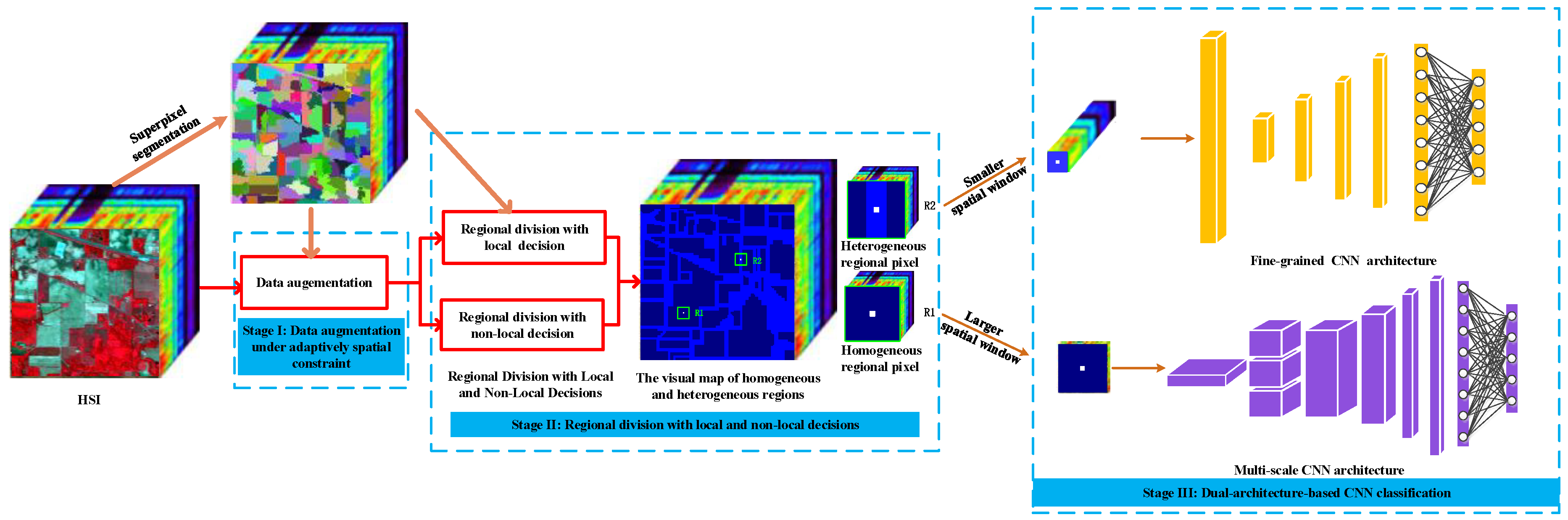
Remotesensing 11 00484 g001
Figure 2. Procedure of the superpixel segmentation.
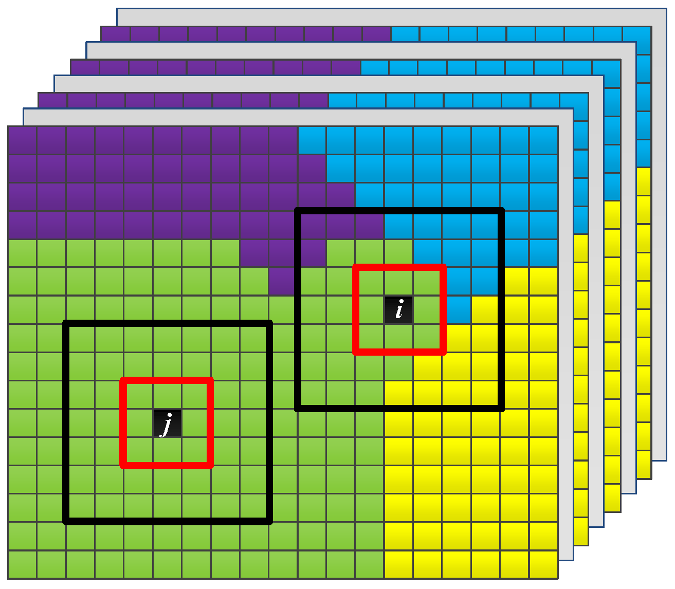
Remotesensing 11 00484 g002
Figure 3. Illustration of samples in the homogeneous and heterogeneous regions.
Remotesensing 11 00484 g003
Figure 4. Illustration of local regional division based on superpixel segmentation: (a) ground truth; (b) superpixel segmentation map; (c) the filter of samples in the homogeneous region; (d) the filter of samples in the heterogeneous region; (e) the filter of samples in the “false boundary”.
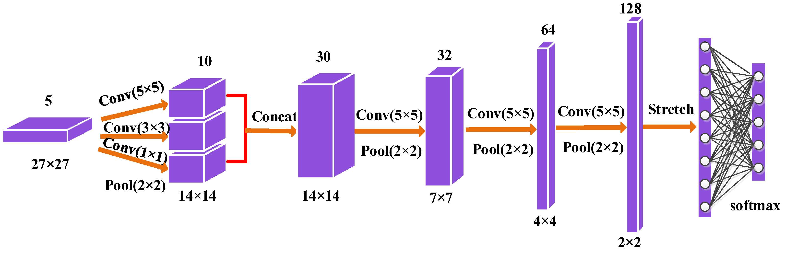
Remotesensing 11 00484 g004
Figure 5. The construction of multi-scale convolutional neural network (CNN).
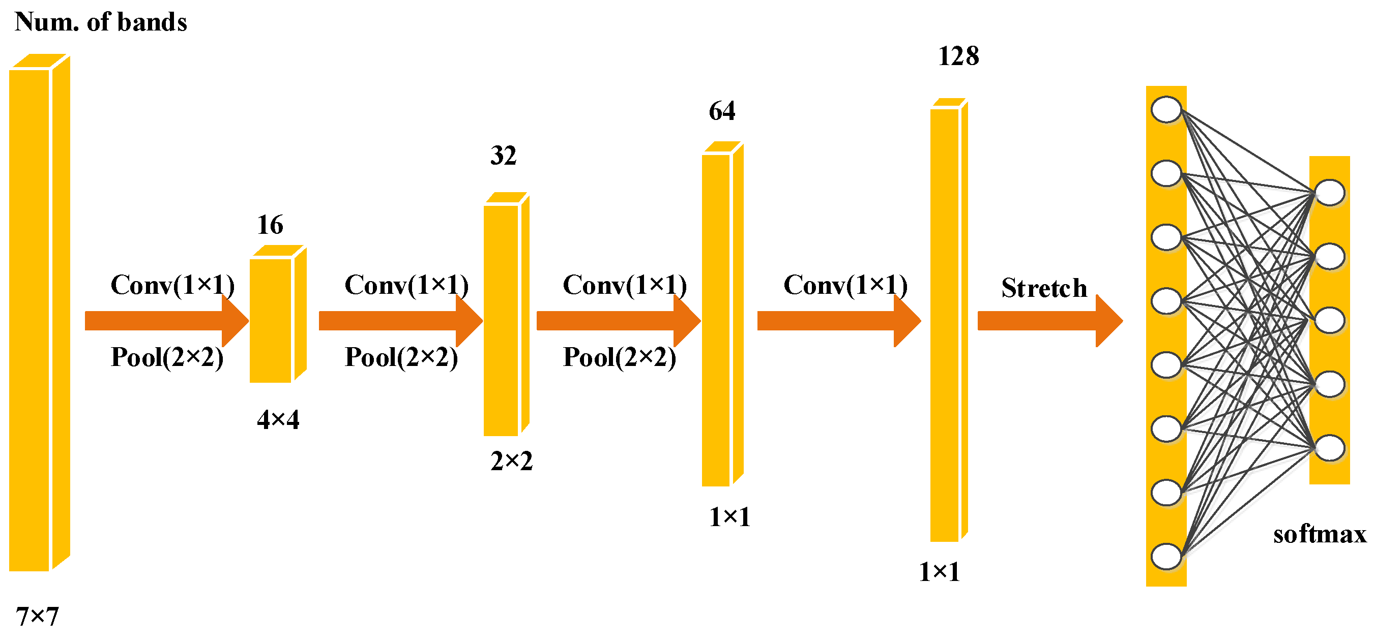
Remotesensing 11 00484 g005
Figure 6. The construction of fine-grained CNN.
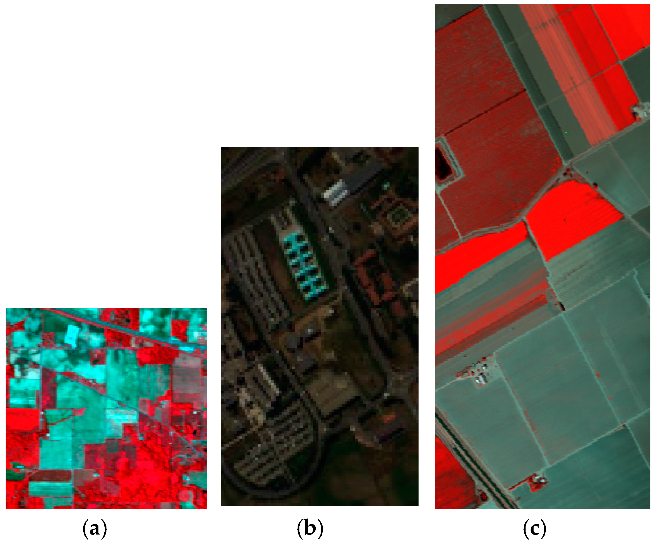
Remotesensing 11 00484 g006
Figure 7. The false-color composite images of (a) the Indian Pines; (b) the Pavia University; (c) the Salinas valley.
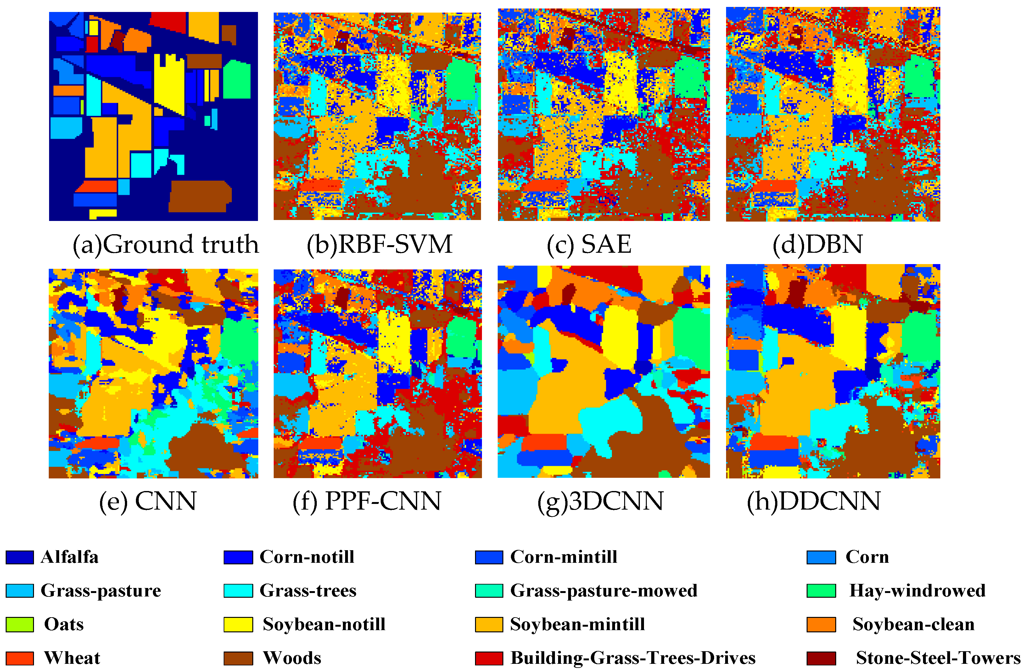
Remotesensing 11 00484 g007
Figure 8. (a) Ground truth and (bh) classification visual maps of the Indian Pines dataset by RBF-SVM, SAE, DBN, PPF-CNN, CNN, 3DCNN, and DDCNN, respectively.
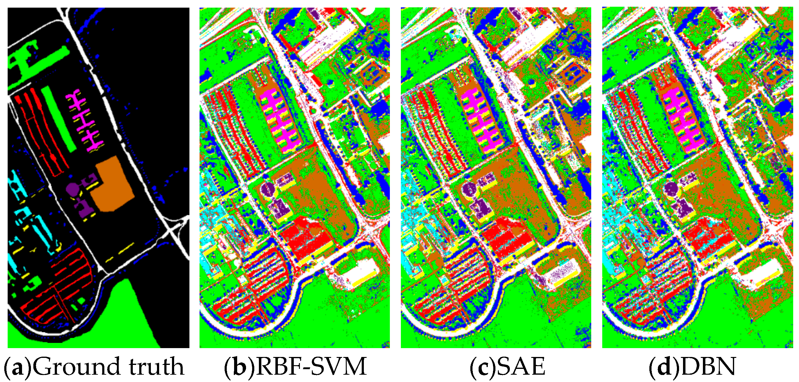
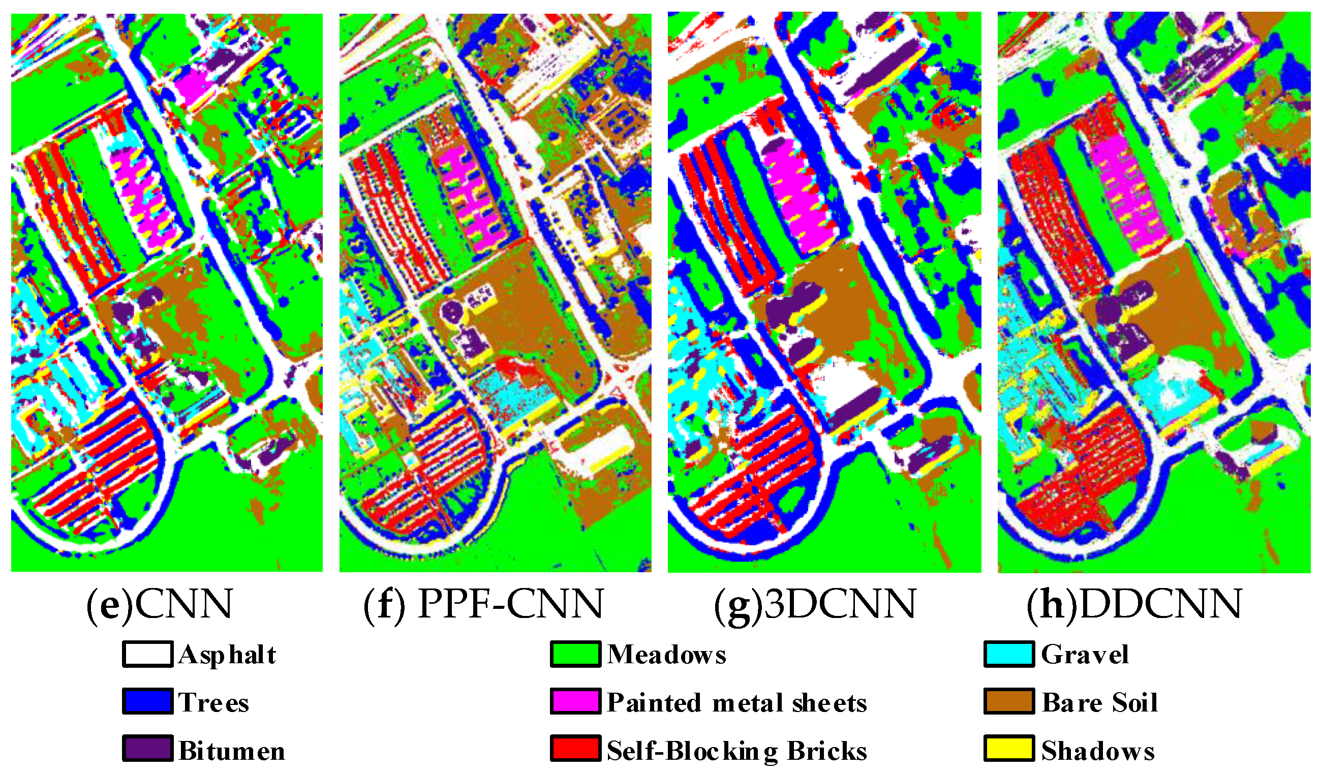
Remotesensing 11 00484 g008
Figure 9. (a) Ground truth and (b–h) classification visual maps of the Pavia University dataset by RBF-SVM, SAE, DBN, CNN, PPF-CNN, 3DCNN, and DDCNN, respectively.
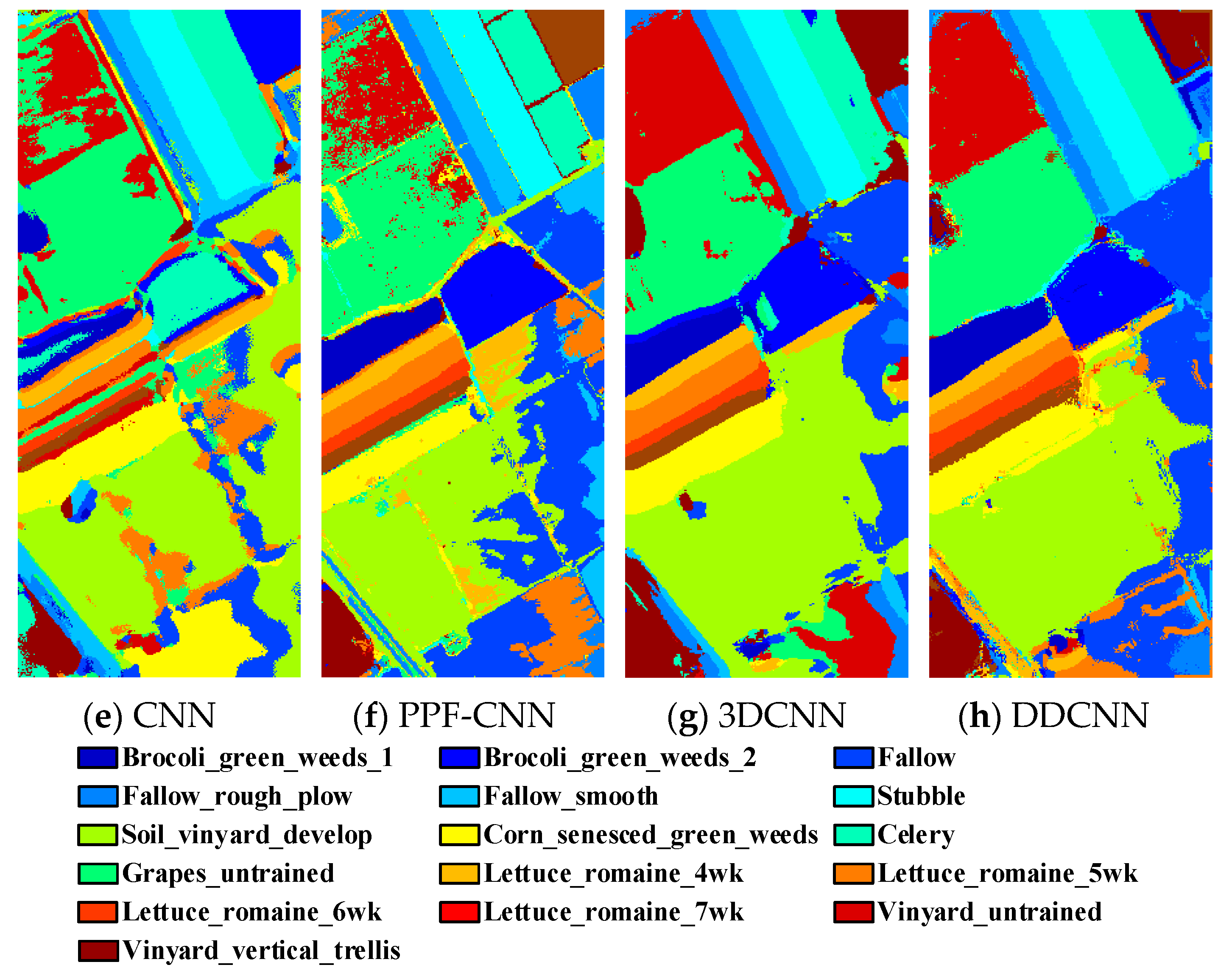
Remotesensing 11 00484 g009aRemotesensing 11 00484 g009b
Figure 10. (a) Ground truth and (b–h classification visual maps of the Salinas dataset by RBF-SVM, SAE, DBN, CNN, PPF-CNN, 3DCNN, and DDCNN, respectively.
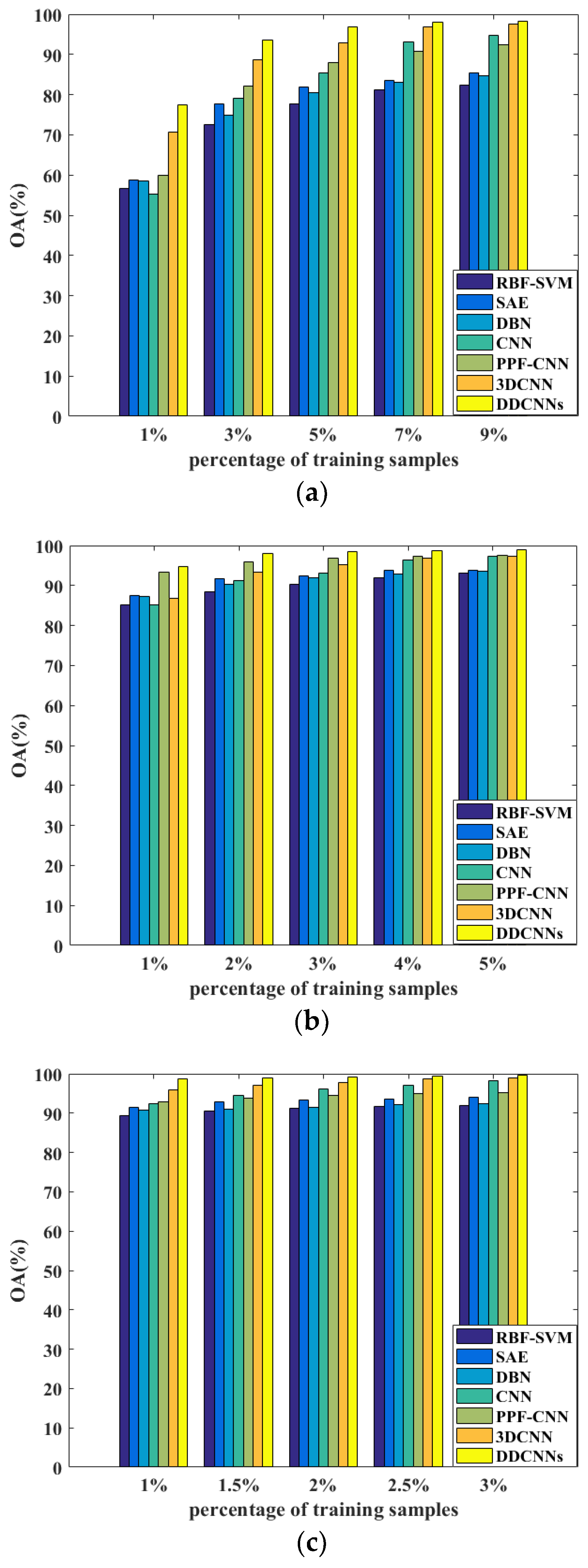
Remotesensing 11 00484 g010aRemotesensing 11 00484 g010b
Figure 11. The OA results of RBF-SVM, SAE, DBN, CNN, PPF-CNN, 3DCNN, and DDCNN with different ratios of training samples on the (a) Indian Pines, (b) Pavia University, and (c) Salinas datasets.
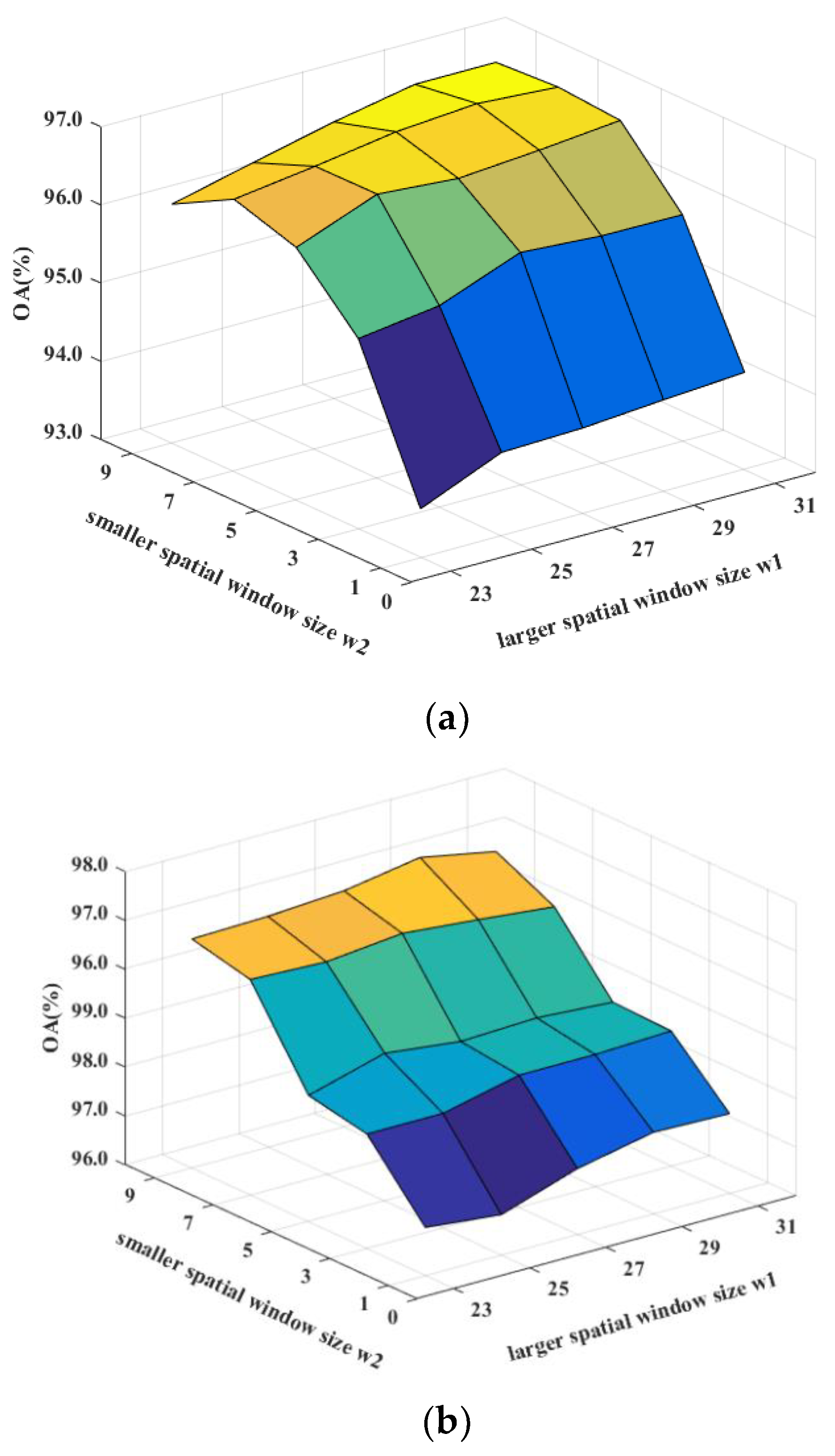
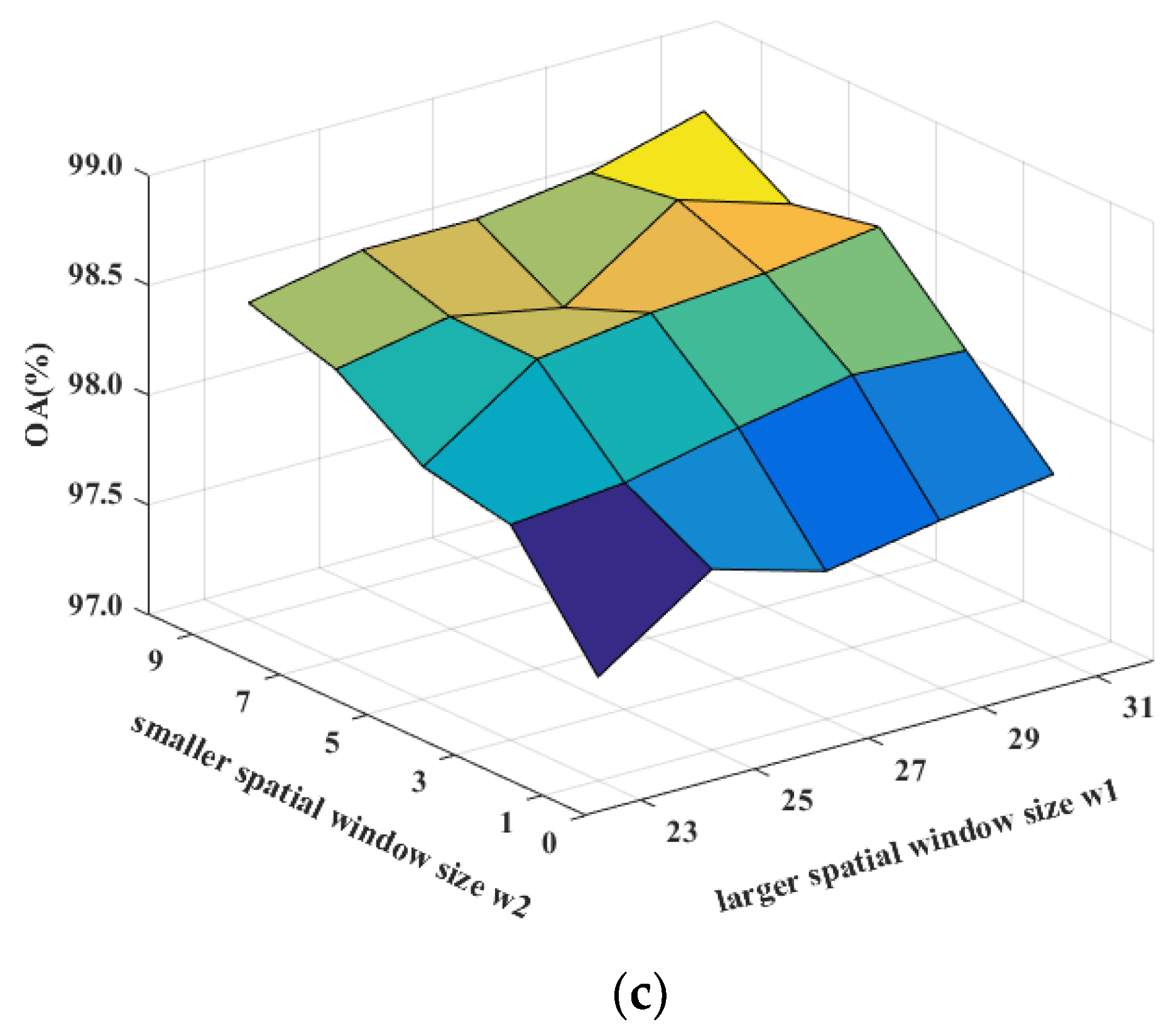
Remotesensing 11 00484 g011
Figure 12. Sensitivity analysis to the spatial window sizes w1 and w2 for DDCNN on (a) the Indian Pines, (b) the Pavia University, and (c) the Salinas datasets.
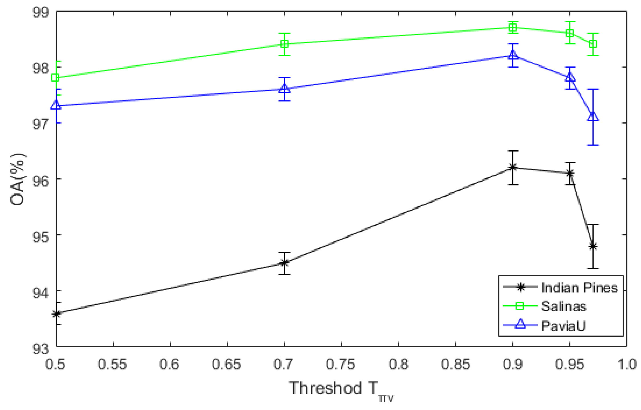
Remotesensing 11 00484 g012aRemotesensing 11 00484 g012b
Figure 13. The sensitivity analysis of DDCNN to the threshold T π v .
Remotesensing 11 00484 g013
Table 1. The procedure of the proposed DDCNN method.
  • INPUT: The training samples X t r a i n and test samples X t e s t from K classes, the class labels of training samples, mini-batch size n, the number of training epochs E
  • Begin
  • Segment the whole HSI into V superpixels { π 1 , π 2 , , π V }
  • The training samples X t r a i n are expanded to new training samples X t r a i n by (7)
  • Training samples X t r a i n are divided into X t r a i n H o and X t r a i n H e , and test samples X t e s t are divided into X t e s t H o and X t e s t H e by (6)
  • initialize all the weight matrices and biases
  • Input the training samples X t r a i n H o
  • for every epoch
  •   for n training sample of every mini-batch
  •    compute the objective function l H o by the cross-entropy loss function
  •    update the parameters of the multi-scale CNN by minimizing loss function
  •   end for
  • end for
  • Input the training samples X t r a i n H e
  • for every epoch
  •   for n training sample of every mini-batch
  •    compute the objective function l H e by the cross-entropy loss function
  •    update the parameters of the multi-scale CNN by minimizing loss function
  •   end for
  • end for
  • Count the labels Y t e s t by Y t e s t H o and Y t e s t H e
  • END
  • OUTPUT: the labels of the test samples classified by the trained DDCNN
Table 2. The 16 Classes of the Indian Pines dataset and the numbers of training and test samples for each class.
ClassNumber of Samples
NoNameTrainingTest
1Alfalfa242
2Corn-notill711286
3Corn-mintill42746
4Corn12213
5Grass-pasture24435
6Grass-trees36658
7Grass-pasture-mowed126
8Hay-windrowed24430
9Oats118
10Soybean-notill49874
11Soybean-mintill1232209
12Soybean-clean30533
13Wheat10185
14Woods631139
15Buildings-Grass-Trees-Drives19348
16Stone-Steel-Towers583
Total5129225
Table 3. Classification results of RBF-SVM, SAE, DBN, CNN, PPF-CNN, 3DCNN, and DDCNN on the Indian Pines dataset.
ClassRBF-SVMSAEDBNCNNPPF-CNN3DCNNDDCNN
16.1±11.210.0±6.413.6±5.678.4±10.250.4±8.483.8±13.499.3±1.6
272.9±3.679.7±2.379.8±2.975.4±2.489.2±2.192.7±3.594.3±2.5
358.0±3.674.9±4.870.5±2.282.8±3.377.1±2.787.2±10.499.0±0.8
439.0±15.062.8±8.371.3±6.689.2±3.587.7±3.783.4±8.395.0±3.3
587.0±4.584.2±3.380.1±4.169.0±4.692.7±1.084.0±5.792.7±2.8
692.4±2.094.3±1.794.2±2.492.8±2.593.1±1.993.4±2.598.8±0.8
70±024.4±18.828.1±22.651.1±12.30±097.2±4.8100.0±0.0
898.1±1.498.8±0.498.5±1.597.1±1.699.6±0.397.4±2.899.8±0.6
90±011.1±10.19.5±2.441.6±9.90±077.0±11.197.8±5.4
1065.8±3.773.6±3.873.2±4.781.0±2.685.6±2.893.3±5.093.8±1.2
1185.3±2.983.4±2.082.7±2.287.2±1.583.8±1.694.9±2.798.1±1.3
1269.6±6.570.4±8.062.0±5.884.4±2.390.4±3.189.8±4.394.4±2.5
1392.3±4.194.2±4.389.7±10.683.1±4.297.8±0.992.8±5.999.9±0.2
1496.6±1.094.2±1.594.4±1.698.2±0.895.5±1.198.3±1.399.5±0.4
1541.7±7.066.1±5.664.2±6.584.7±4.578.0±2.477.8±13.495.7±2.6
1675.2±9.087.6±8.180.5±13.276.0±8.197.3±1.388.4±5.389.7±9.4
OA (%)77.8±0.881.9±0.180.6±0.185.4±0.887.9±0.892.8±0.896.9±0.6
AA (%)61.3±1.469.4±1.968.3±1.779.4±1.676.5±0.689.4±1.496.6±0.7
Kappa (%)74.5±1.079.3±1.177.8±1.384.3±2.986.3±0.991.9±0.996.3±0.8
Table 4. 9 Classes of the Pavia University dataset and the numbers of training and test samples for each class.
ClassNumber of Samples
NoNameTrainingTest
1Asphalt1996233
2Meadows55917531
3Gravel631973
4Trees922880
5Painted metal sheets401265
6Bare Soil1514727
7Bitumen401250
8Self-Blocking Bricks1103462
9Shadows28891
Total128240212
Table 5. Classification results of RBF-SVM, SAE, DBN, CNN, PPF-CNN, 3DCNN, and DDCNN on the Pavia University dataset.
ClassRBF-SVMSAEDBNCNNPPF-CNN3DCNNDDCNN
190.7±1.192.3±1.191.6±0.893.1±1.498.0±0.195.5±1.297.8±1.1
296.8±0.797.6±0.397.4±0.497.6±0.999.2±0.299.4±0..399.5±0.1
360.2±5.472.1±3.569.7±6.077.9±4.584.9±1.892.6±5.498.4±0.9
490.8±2.090.9±1.491.2±1.486.4±3.695.8±0.875.2±4.995.9±1.1
598.8±0.498.7±0.498.6±0.698.5±1.499.8±0.195.4±4.399.4±0.5
679.5±4.986.9±1.985.6±2.291.0±2.896.4±0.399.4±0.699.7±0.3
774.3±5.178.1±4.974.8±4.881.2±2.989.2±0.891.5±3.499.6±0.4
888.8±2.287.8±1.488.2±1.392.5±2.293.7±1.294.8±1.497.8±1.3
999.8±0.199.5±0.399.6±0.179.0±4.198.5±0.777.4±2.887.9±2.5
OA (%)90.3±0.692.4±0.391.9±0.393.0±0.696.9±0.295.2±0.798.5±0.2
AA (%)86.6±0.989.3±0.788.5±0.888.6±0.895.1±0.291.2±1.197.3±0.4
Kappa (%)87.1±0.889.9±0.489.2±0.490.7±0.796.0±0.293.8±0.998.1±0.2
Table 6. The 16 Classes of the Salinas dataset and the numbers of training and test samples for each class.
CategoryNumber of samples
NoNameTrainingTest
1Brocoli_green_weeds_1201969
2Brocoli_green_weeds_2373652
3Fallow201936
4Fallow_rough_plow141366
5Fallow_smooth272624
6Stubble403879
7Celery363507
8Grapes_untrained11311045
9Soil_vinyard_develop626079
10Corn_senesced_green333212
11Lettuce_romaine_4wk111046
12Lettuce_romaine_5wk191889
13Lettuce_romaine_6wk9898
14Lettuce_romaine_7wk111048
15Vinyard_untrained737122
16Vinyard_vertical181771
Total54353043
Table 7. Classification results of RBF-SVM, SAE, DBN, CNN, PPF-CNN, 3DCNN, and DDCNN on the Salinas dataset.
ClassRBF-SVMSAEDBNCNNPPF-CNN3DCNNDDCNN
197.4±1.597.9±0.598.5±0.893.3±8.798.5±0.588.6±3.5100.0±0.0
299.7±0.299.1±0.598.9±0.297.4±1.299.7±0.294.5±2.999.8±0.2
393.7±1.595.3±0.697.5±0.186.4±4.199.8±0.191.4±4.799.7±0.4
497.8±1.399.5±0.699.0±0.398.2±1.899.7±0.296.8±2.198.3±0.8
597.5±1.198.5±0.497.5±0.298.1±1.096.8±0.296.7±2.799.3±0.5
699.5±0.399.9±0.199.3±0.199.9±0.299.8±0.398.5±1.299.9±0.2
799.3±0.299.2±0.199.0±0.399.0±0.999.5±0.298.0±1.399.9±0.1
888.9±2.982.7±0.783.0±1.488.4±2.889.9±0.992.3±1.199.4±0.3
999.2±0.399.2±0.199.0±0.195.1±0.7 99.8±0.298.9±0.499.9±0.1
1088.8±1.988.9±0.992.8±0.193.6±2.488.3±2.799.1±0.895.3±1.2
1187.5±4.693.6±7.091.7±0.197.6±1.093.4±2.997.6±2.199.8±0.2
1298.0±2.398.6±1.099.0±0.198.9±1.199.7±0.796.6±2.798.6±0.9
1398.0±0.899.2±0.799.3±0.294.7±2.498.6±0.790.9±0.799.7±0.2
1489.6±2.694.8±0.292.0±7.492.5±3.992.3±1.798.2±1.093.8±1.8
1553.9±7.675.9±2.469.5±0.280.1±5.372.9±2.598.6±0.896.6±0.5
1690.8±5.096.1±1.996.1±2.593.6±2.695.7±1.896.3±3.098.0±1.0
OA (%)89.3±0.791.5±0.190.8±0.692.3±1.292.8±0.495.9±0.298.8±0.2
AA (%)92.5±0.694.9±0.294.5±0.894.2±0.995.5±0.795.8±0.298.6±0.2
Kappa (%)88.0±0.890.6±0.489.7±0.791.4±1.491.9±0.495.5±0.298.6±0.2
Table 8. Running time and Parameters of RBF-SVM, SAE, DBN, CNN, PPF-CNN, 3DCNN, and DDCNN on the Indian Pines dataset.
DatasetMethodTraining Time (s)Test Time (s)Parameters
Indian PinesRBF-SVM0.4±0.11.2±0.1200
SAE76.3±8.40.2±0.126160
DBN114.3±20.10.2±0.124060
CNN220.7±27.90.5±0.181408
PPF-CNN2056.0±36.75.3±0.361870
3DCNN2690.2±57.916.0±0.144961792
DDCNN587.2±22.70.7±0.1376932
Table 9. Running time and Parameters of RBF-SVM, SAE, DBN, CNN, PPF-CNN, 3DCNN, and DDCNN on the Pavia University dataset.
DatasetMethodTraining Time (s)Test Time (s)Parameters
Pavia UniversityRBF-SVM0.5±0.13.5±0.1200
SAE82.2±5.30.3±0.119920
DBN147.0±10.60.4±0.221420
CNN371.8±15.31.2±0.161249
PPF-CNN4367.9±29.57.2±0.461310
3DCNN1979.0±12.631.4±5.55866224
DDCNN682.1±10.62.3±0.1375140
Table 10. Running time and Parameters of RBF-SVM, SAE, DBN, CNN, PPF-CNN, 3DCNN, and DDCNN on the Salinas dataset.
DatasetMethodTraining Time (s)Test Time (s)Parameters
SalinasRBF-SVM0.4±0.12.7±0.1204
SAE70.1±2.40.6±0.126160
DBN102.6±9.10.5±0.224060
CNN165.1±2.10.7±0.182216
PPF-CNN1940.1±17.464.6±1.561870
3DCNN1157.7±25.728.1±0.45867520
DDCNN657.2±20.64.7±0.2376932
Table 11. Classification results of CNN, RPCA-CNN, DCNN, and DDCNN on the Indian Pines, Pavia University, and Salinas Datasets.
Data setClassification IndexCNNRPCA-CNNDCNNDDCNN
Indian Pines DatasetOA (%)85.4±0.888.6±0.693.4±0.596.9±0.6
AA (%)79.4±1.682.6±2.389.5±1.796.6±0.7
Kappa (%)84.3±2.986.1±0.792.5±0.596.3±0.8
Pavia University DatasetOA (%)93.0±0.694.2±0.295.7±0.898.5±0.2
AA (%)88.6±0.891.6±0.295.3±0.897.3±0.4
Kappa (%)90.7±0.792.4±0.595.2±0.998.1±0.2
Salinas DatasetOA (%)92.3±1.292.9±0.694.5±0.698.8±0.2
AA (%)94.2±0.994.2±0.994.5±0.698.6±0.2
Kappa (%)91.4±1.491.4±1.493.9±0.798.6±0.2
Table 12. Classification results of DDCNN, MCNN, FCNN, and DDCNN-WDA on the Indian Pines, Pavia University, and Salinas Datasets.
Data setClassification IndexDDCNNFCNNMCNN DDCNN-WDA
Indian Pines DatasetOA (%)96.9±0.693.3±0.795.8±0.595.9±0.7
AA (%)96.6±0.790.6±2.192.6±1.993.2±2.0
Kappa (%)96.3±0.892.4±0.895.3±0.695.3±0.8
Pavia University DatasetOA (%)98.5±0.297.4±0.297.8±0.497.7±0.9
AA (%)97.3±0.495.9±0.595.5±1.195.9±0.9
Kappa (%)98.1±0.296.6±0.397.1±0.596.9±1.3
Salinas DatasetOA (%)98.8±0.296.3±0.797.1±1.598.4±0.3
AA (%)98.6±0.297.4±0.597.1±1.797.7±0.6
Kappa (%)98.6±0.295.9±0.996.8±1.797.9±1.4
Table 13. The sensitivity analysis of numbers of convolutional layers.
DatasetClassification Indexthe Number of Convolutional Layers
12345
Indian Pines DatasetOA (%)93.6±0.495.5±0.496.0±0.196.9±0.696.4±0.3
AA (%)91.6±1.194.5±0.395.5±0.396.6±0.795.3±0.7
Kappa (%)92.8±0.494.9±0.495.4±0.196.3±0.895.8±0.4
Pavia University DatasetOA (%)95.8±0.197.4±0.298.7±0.198.5±0.298.4±0.1
AA (%)95.1±0.496.7±0.398.3±0.197.3±0.498.2±0.2
Kappa (%)94.5±0.196.6±0.398.4±0.298.1±0.297.8±0.1
Salinas DatasetOA (%)94.3±0.295.5±0.698.5±0.298.8±0.298.6±0.2
AA (%)96.2±0.397.1±0.598.5±0.298.6±0.298.5±0.3
Kappa (%)93.7±0.395.1±0.798.4±0.298.6±0.298.5±0.2
Table 14. The sensitivity analysis of numbers of superpixels in DDCNN.
DatasetClassification IndexThe Number of Superpixels
5010050010005000
Indian Pines DatasetOA (%)94.7±0.496.9±0.696.3±0.393.7±0.392.7±0.5
AA (%)92.1±1.696.6±0.795.4±0.991.6±1.891.1±1.3
Kappa (%)94.0±0.496.3±0.895.8±0.392.8±0.491.4±0.9
Pavia University DatasetOA (%)97.1±0.297.5±0.298.3±0.198.5±0.297.3±0.3
AA (%)95.5±0.496.9±0.297.8±0.197.3±0.496.3±0.2
Kappa (%)96.4±0.396.7±0.397.8±0.198.1±0.296.4±0.5
Salinas DatasetOA (%)97.2±0.498.8±0.297.3±0.495.9±0.994.9±0.5
AA (%)96.5±1.098.6±0.296.7±0.494.5±1.692.9±0.8
Kappa (%)96.9±0.598.6±0.297.0±0.495.5±0.994.9±0.5

