The 2014–2015 Lava Flow Field at Holuhraun, Iceland: Using Airborne Hyperspectral Remote Sensing for Discriminating the Lava Surface

Abstract

The Holuhraun lava flow was the largest effusive eruption in Iceland for 230 years, with an estimated lava bulk volume of ~1.44 km³ and covering an area of ~84 km². The six month long eruption at Holuhraun 2014–2015 generated a diverse surface environment. Therefore, the abundant data of airborne hyperspectral imagery above the lava field, calls for the use of time-efficient and accurate methods to unravel them. The hyperspectral data acquisition was acquired five months after the eruption finished, using an airborne FENIX-Hyperspectral sensor that was operated by the Natural Environment Research Council Airborne Research Facility (NERC-ARF). The data were atmospherically corrected using the Quick Atmospheric Correction (QUAC) algorithm. Here we used the Sequential Maximum Angle Convex Cone (SMACC) method to find spectral endmembers and their abundances throughout the airborne hyperspectral image. In total we estimated 15 endmembers, and we grouped these endmembers into six groups; (1) basalt; (2) hot material; (3) oxidized surface; (4) sulfate mineral; (5) water; and (6) noise. These groups were based on the similar shape of the endmembers; however, the amplitude varies due to illumination conditions, spectral variability, and topography. We, thus, obtained the respective abundances from each endmember group using fully constrained linear spectral mixture analysis (LSMA). The methods offer an optimum and a fast selection for volcanic products segregation. However, ground truth spectra are needed for further analysis.

1. Introduction

Lava flow emplacement is an important constructive geological process that contributes to reshaping natural landscapes [1,2,3]. To assess the hazards and long-term impacts posed by lava flows, it is vital to understand aspects such as the return period of effusive eruptions, to map the areas covered by eruptions in the past and to characterize the evolution of lava flow surfaces after emplacement [4,5]. In high eruption frequency areas, lava flows often overlap each other. If the overlapping lava flows erupt within a short time span and have similar chemical and surface characteristics, discrimination will be further complicated by their similar spectral signatures. Spectral reflectance plays an important role in visible and shortwave infrared (VIS-SWIR) remote sensing. Each material absorbs and reflects the incoming radiation in a characteristic way. In the 400–2500 nm range, minerals display absorption features due to the interaction of light with cations (Fe, Mg, Al) and anions (OH, CO₃) [6]. Reflectance spectra provide information about the specific material and their composition. They are used for different applications such as classification of remotely sensed data, identification of mineral features of rock, and environmental assessment [7,8]. The interest in reflectance spectra of volcanic rocks has increased recently as they can play an important role as planetary analogues. In fact, these spectra can be used to identify compounds by data acquired by ongoing solar system exploration missions [9,10].

Characterization of surface spectral reflectance by satellite remote sensing is constrained by the spectral range and resolution (i.e., number of spectral bands) as well as by the spatial resolution of the imagery. Whereas multispectral imagery can be acquired at very high spatial resolution (e.g., WorldView [11,12]); the spatial resolution of hyperspectral satellite data remains low (e.g., EO-1 Hyperion with a ground resolution of 30 m x 30 m); and spectral mixing is thus a major issue [13]. The spectral reflectance of lava of different compositions has also been documented using laboratory spectrometry with decimeter-size samples [14]. For accessible volcanic terrains, field spectrometry offers a useful alternative approach for characterizing the spectral reflectance of contrasted lava surfaces and for documenting its spatial variation at different spatial scales [5,14]. The great variety of morphologies observed in the 2014–2015 Holuhraun lava flows [1,15] encouraged a detailed study of their spectral characteristics, to obtain information about lava composition and detect possible differences in the spectra of the flow. In spectroscopy, the identification of the mineral constituents of major rock types is typically approached using spectral unmixing methods [5,16]. Usually, in the visible and near-infrared spectral range, mafic rocks are characterized by very low reflectance due to the presence of large amounts of dark mafic minerals [14]. The 2014–2015 lava flow at Holuhraun in NE Iceland offers an excellent diverse surface environment for investigating and characterizing lava deposits. Its intense volcanic activity [1,17,18,19], geomorphological complexity [20], and well-documented flank eruptions [1] perplex the remote sensing monitoring of the bulk volcanic edifice. However, the detailed field mapping of lithologies is frequently obstructed by difficulties in accessibility, the scale of lava flow fields, topography, while remote sensing has become increasingly important in mapping volcanic terrains and specifically in mapping lava flows. Mapping individual lava flows using satellite remote sensing is challenging for at least three reasons: vegetation cover, spatial overlapping, and spectral similarity [3,4]. Moreover, a high eruption frequency often leads to lava flows overlapping each other. If the overlapping lava flows are erupted within a short period and have similar chemical and surface characteristics, discrimination will be further complicated by their similar spectral signatures.

Hyperspectral remote sensing provides information on hundreds of distinct and contiguous channels of the electromagnetic spectrum, thus enabling the identification of multiple ground objects through their detailed spectral profiles. However, restrictions on the spatial resolution of hyperspectral data, the multiple scattering of the incident light between objects, and microscopic material mixing form the mixed pixel problem. Pixels are identified as mixed when they are composed of the spectral signatures of more than one ground object. Therefore, we adopted linear spectral mixture analysis (LSMA) techniques [8,21], which model the pixel spectra as a combination of pure components (endmembers) weighted by the fractions (abundances) that contribute to the total reflectance of the mixed pixel [22]. Ideally, each selected endmember from the hyperspectral image under study has the maximum possible abundance of a single physical material present and minimum abundance of the rest of the physical materials. Spectral unmixing typically consists of two main substages: (a) endmember extraction; and (b) abundance estimation [22]. In this paper, we focus on both endmember extraction and estimation of fractional abundances of the lava field products on 2014–2015 Holuhraun lava fields. For this purpose, an airborne hyperspectral image with an AisaFENIX sensor on board a NERC Airborne Research Facility (Natural Environment Research Council Airborne Research Facility) campaign was acquired at Holuhraun after the eruption and for the sub-pixel analysis we used the sequential maximum angle convex cone (SMACC) algorithm to identify the spectral image endmembers while the LSMA method was employed to retrieve the abundances. Our approach was narrowed to the eruptive fissure vent part since it is considered to have a more diverse surface. The resulting abundances from the LSMA method were both quantitatively and qualitatively compared with the spectral indices technique, aerial and field photographs, respectively. The objective was to retrieve the main lava surface type contributing to the signal recorded by airborne hyperspectral at the very top surface of Holuhraun.

2. The 2014–2015 Eruption at Holuhraun

The eruption took place in the tectonic fissure swarm between the Bárðarbunga-Veiðivötn and the Askja volcanic systems (Figure 1a). It lasted about six months (31 August 2014 to 27 February 2015) and produced a bulk volume ~1.44 km³ of basaltic lava [1]. Lava effusion rates during the eruption period range from 320 to 10 m³/s. Averaged values are ∼250, 100, and 50 m³/s during the initial (August–September 2014), intermediate (October–December 2014) and final phase (December 2014 to February 2015), respectively [1,17] (Figure 1b). The lava was emplaced on the sandur plains (glacial outwash sediment plains) north of the Vatnajökull/Dyngjujökull glacier, partially covering the previous two Holuhraun lava flow fields south of the Askja caldera [1]. The area is gently sloping (average inclination <0.5%; i.e., ∼0.3°) to the east-northeast. The shallow gradient resulted in low topographic forcing of the flow and, therefore, rather slow lava flow advance. During its emplacement history, the lava field was initially dominated by channels and horizontal expansion. Then it transitioned to grow in volume primarily by inflation, tube-fed flow (i.e., transport of lava through roofed over partially or filled channels) and vertical stacking of lava-lobes. The 2014–2015 effusive eruption products originate from intense activity in the vent, in which high oxidation occurs in this area. The main lava channel shows significant inflation (5–10 m). Lava advancement rates were generally low ∼0.0167 m/s during the initial eruption phase [1] and dropped to ∼0.0017 m/s during the middle of November 2014 [23]. The six-month-long effusive eruption features diverse surface structures and morphologies. The 2014–2015 lava flow at Holuhraun in NE Iceland offers an excellent diverse surface environment to investigate and characterize lava deposits.

3. Spectral Unmixing on Lava

Various spectroscopy studies [2,5,7,14,25] over the volcanic area have examined the mineralogical composition of the extensive lava fields. Usually, in the visible (VIS) and near-infrared (NIR) spectral range, mafic rocks are characterized by very low reflectance due to the presence of large amounts of dark mafic minerals [14]. Spectral indices provide the first efficient way to emphasize subtle spectral variations at the surface [26]. More elaborate methods have been developed to discriminate and quantify mixtures of mafic minerals. They have been used to derive composition maps of mafic minerals [27,28,29]. However, some lava flows can have a similar chemical/mineralogical composition but dissimilar spectral behaviour due to the different grain size, surface texture, and presence of weathering [13,14]. The main components of igneous rocks do not display any peculiar spectral features in the visible and near infrared spectral range. In the case of basalts, the only spectral feature commonly found is an absorption peak, due to iron, located around 1000 nm [26]. However, in the case of hydrothermal alteration, hydroxyl bearing minerals show distinctive absorption features in the 2000–2500 nm spectral region [30]. Because of the heterogeneity of the lava surface, mixed pixels are very common which is illustrated in Figure 2a,b.

Spectral Mixing Analysis (SMA) has been specifically developed to account for mixtures [10]. Analysis of the data sample can simply be performed on these abundance fractions rather than the sample itself. This method is well-suited for spectroscopic analysis because most of the spectral shapes are due to different materials. The signal detected by a sensor at a single pixel is frequently a combination of numerous disparate signals. Unmixing techniques were applied to the volcano of Nyamuragira for discriminating lava flows of different ages by Li et al. [5]. The most recent study by Daskalopoulou et al. [16], used unmixing techniques to segregate lava flows and related products from the historical Mt. Etna. Nonetheless, there are no findings concerning lava flow delineation through unmixing in Iceland.

4. Data Acquisitions and Methods

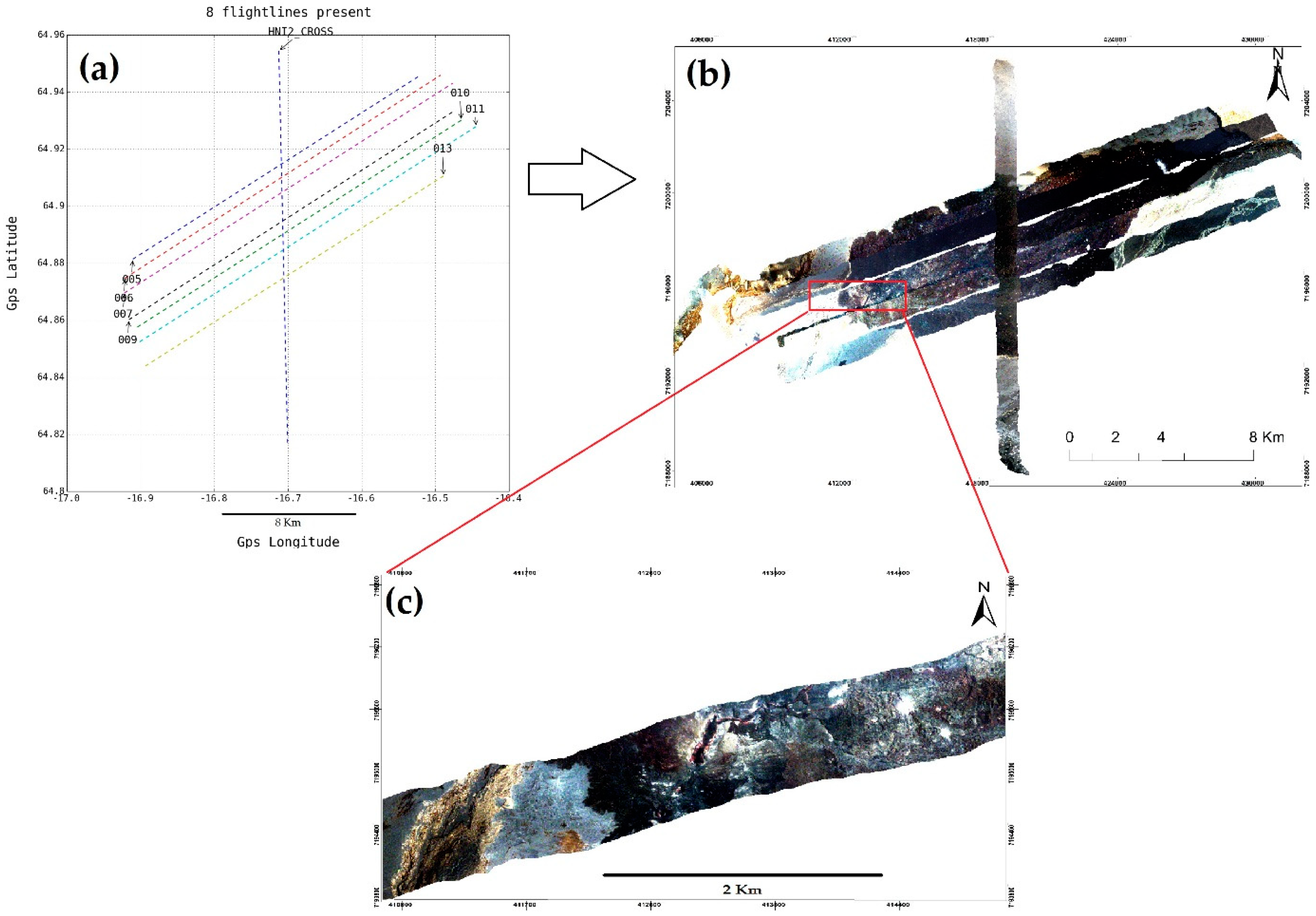
4.1. Airborne Hyperspectral Data Acquisitions

Airborne hyperspectral data were acquired on 4 September 2015 between 16.56 and 17.58 (local time) with an AisaFENIX sensor (Specim, Spectral Imaging Ltd, http://www.specim.fi) [31] on board a NERC Airborne Research Facility (Natural Environment Research Council Airborne Research Facility http://www.bas.ac.uk/nerc-arf) aircraft [32]. Pushbroom VNIR and SWIR sensor, are two separate detectors with common fore-optics. The hyperspectral data contain 622 channels with spectral range from ~400 nm to 2500 nm (break at ~970 nm). The pixel size of this data is explained in Section 4.2.2. In total, eight flights were acquired at the Holuhraun lava flow during this period with an average altitude of 2.4 km (Figure 3a). The data are delivered as level 1b ENVI BIL format files which means that radiometric calibration algorithms have been applied and navigation information has been synced to the image data (Figure 3b). In this study, we subset the data to focus on the area around the eruptive fissures vent (Figure 3c) which is thought to have a diverse surface and has field photographs. Very high-resolution aerial photographs of the lava field (0.5 m spatial resolution) from Loftmyndir ehf (http://www.loftmyndir.is/) [33] were used for comparison and validation of the unmixing results.

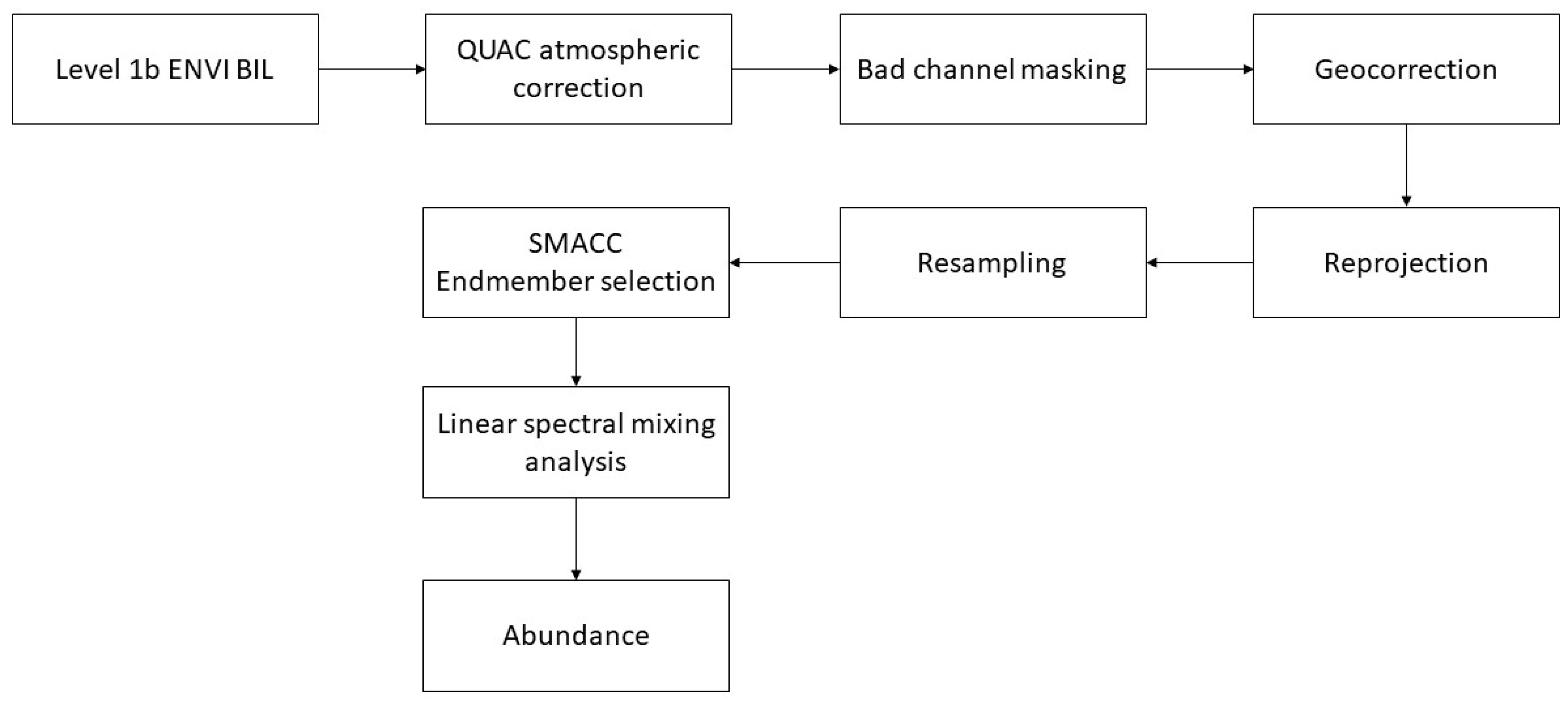
4.2. Spectral Unmixing and Abundance Retrieval

The processing workflow towards unmixing and generating abundance consists of four steps: (1) Atmospheric correction to retrieve surface reflectance; (2) Data masking, geocorrection, reprojection, and resampling; (3) An endmember selection algorithm was adopted to select the endmembers; then a linear spectral mixing analysis method was employed to retrieve the abundance (Figure 4).

4.2.1. Atmospheric Correction

Remote-sensing applications require removing the atmospheric effect from the imagery, to retrieve the spectral reflectance of the surface materials. In this study, the data were atmospherically corrected using the quick atmospheric correction (QUAC) algorithm [34,35], since we had no prior knowledge to perform empirical calibration [36,37]. QUAC is an in-scene approach, requiring only an approximate specification of sensor band locations (i.e., central wavelengths) and their radiometric calibration; no additional metadata is required [35]. QUAC does not involve first principles radiative transfer calculations, and therefore it is significantly faster than physics-based methods; however, it is also more approximate [35].

4.2.2. Data Masking, Geocorrection, Reprojection, and Resampling

In this study, we use the Airborne Processing Library (APL) software for processing the data [38]. The first step of the APL processing is to apply the mask of bad channels to atmospherically corrected data, creating a new file with bad channels set to zero (Appendix A on Figure A1). The next step uses the navigation file, the view vector file, and the digital elevation file (DEM) to calculate the ground position for each pixel then change the projection to UTM (Universal Transverse Mercator) Zone 28N [38]. We used satellite-based ASTER sensor for the DEM. In the final step we resampled output pixel size to ~3.5 m according to the height above ground level (AGL) that is given by the theoretical pixel size chart that can be found in Appendix A on Figure A2 (https://nerc-arf-dan.pml.ac.uk/trac/wiki/Processing/PixelSize) [39].

4.2.3. Endmembers Selection

The conventional image-based endmember selection approach based on scatterplots of the image bands may not be effective in identifying a sufficient number of endmembers. In this paper, we employed the sequential maximum angle convex cone (SMACC) algorithm [34] to identify spectral image endmembers. Endmembers are spectra that represent pure surface materials in a spectral image. The extreme points were used to determine a convex cone, which defined the first endmember. A constrained oblique projection was applied to the existing cone to derive the next endmember. The cone was then increased to include a new endmember [8,40]. This process was repeated until a projection derived an endmember that already existed within the convex cone, or until a specified number of endmembers was satisfied [21]. When implemented with SMACC, the output endmember number was set as 5, 10, 15, 20, and 30 respectively. Better endmembers could be identified easily from the 15 endmembers output (more detail in Section 6.2). Then, we used the selected 15 endmembers for deriving the abundance.

4.2.4. Linear Spectral Mixture Analysis

The linear spectral mixture analysis (LSMA) approach was adopted to calculate the abundance of endmembers for each pixel. LSMA assumes that the spectrum measured by a sensor is a linear combination of the spectra of all components (endmembers) within the pixel, and the spectral proportions of the endmembers (i.e., their abundance) reflect the proportion of area covered by distinct features on the ground [8,21]. The general equation for linear spectral mixing can be expressed as:

$${\mathit{R}}_{\mathit{i}\mathit{j},\mathit{\lambda }}={\displaystyle \sum _{\mathit{n}=1}^{\mathit{N}}{\mathit{p}}_{\mathit{i}\mathit{j},\mathit{n}}{\mathit{R}}_{\mathit{n},\mathit{\lambda }}+{\mathit{E}}_{\mathit{\lambda }}}$$

(1)

where R_ij,λ is the measured reflectance at wavelength λ for pixel ij, where i is the column pixel number, and j is the line pixel number; p_ij,n is the fraction of endmembers n contributing to the image spectrum of pixel ij; N is the total number of endmembers; R_n,λ is the reflectance of endmember n at wavelength λ; and E_λ is the error at wavelength λ of the fit of N spectral endmembers. The fraction p_ij,n can be solved using a least-square method with fully constrained unmixing. Fully constrained unmixing means that the sum of the endmember fractional (abundance) values for each pixel must equal unity, which requires a complete set of endmembers. Therefore, it should meet the following two conditions:

$$0\le {\mathit{p}}_{\mathit{i}\mathit{j},\mathit{n}}\le 1$$

(2)

$${\displaystyle \sum _{\mathit{n}=1}^{\mathit{N}}{\mathit{p}}_{\mathit{i}\mathit{j},\mathit{n}}=1}$$

(3)

In the majority of cases, the unmixing is only partially constrained because the extracted endmember set is incomplete for the image and only term (2) (i.e., Equation (2)) is satisfied. In this study, fully constrained LSMA were applied to the FENIX image to obtain the abundance result and both SMACC and LSMA were executed by ENVI 5.3 and IDL 8.5 language programming.

5. Results

5.1. Endmember Groups

The approximate locations of the 15 endmembers selected are shown in Figure 5a. SMACC first finds the brightest spectral in the image and defines it as the first endmember. In this study, the first endmember (endmember 1) represented saturated hot material. We grouped these 15 endmembers into six groups; (1) basalt; (2) hot material; (3) oxidized surface; (4) sulfate mineral; (5) water; and (6) noise (Figure 5b–g). These groups were based on the similar shape of the endmembers with the USGS spectral library; however, the amplitude of the endmembers within a group vary due to illumination conditions, spectral variability, and topography. We added up the abundances within the group to derive the abundance according to this endmembers group.

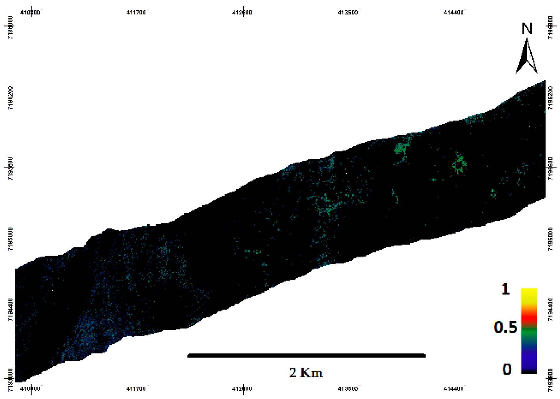
5.2. Basalt Abundance

Figure 6a indicates the presence of the dominant basalt abundance pixel throughout the image. This abundance is associated with endmember 8 which is characterized by very low reflectance (Figure 5b) due to the presence of large amounts of dark mafic rock since the study area is dominated by basaltic lava (Figure 6b).

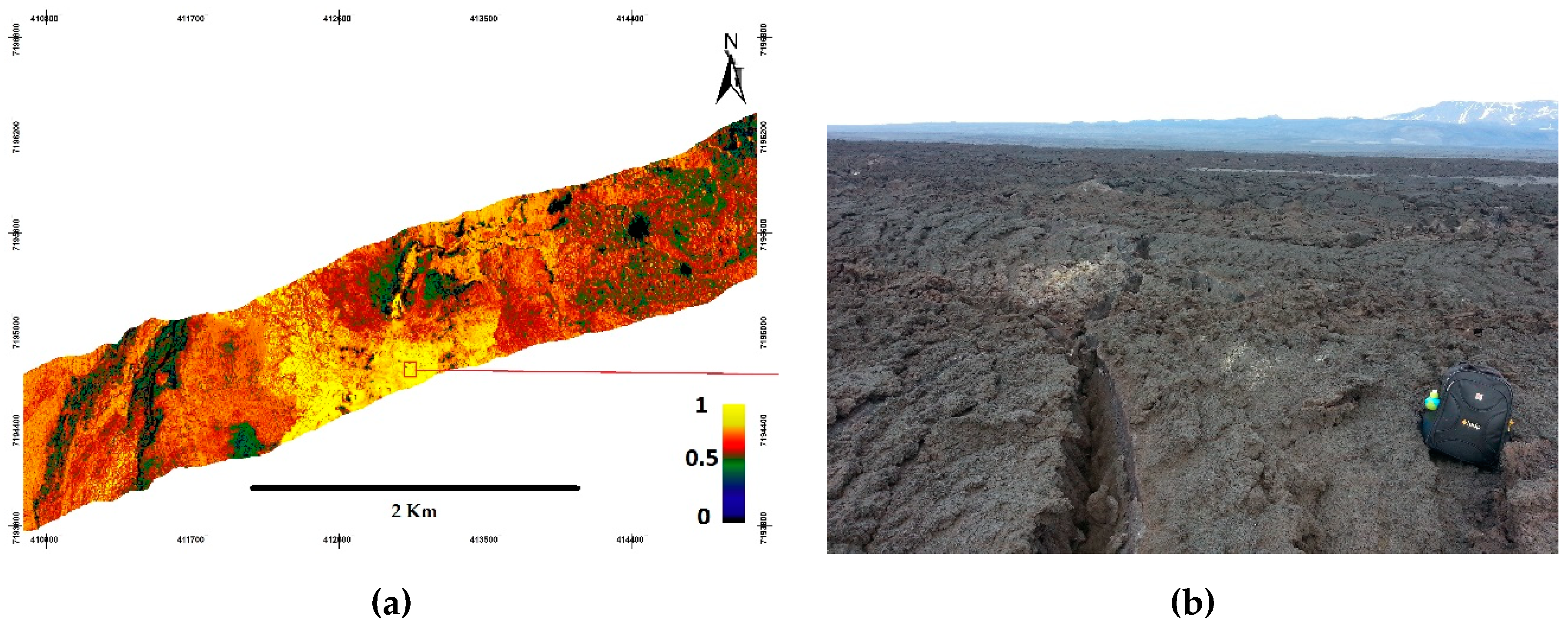
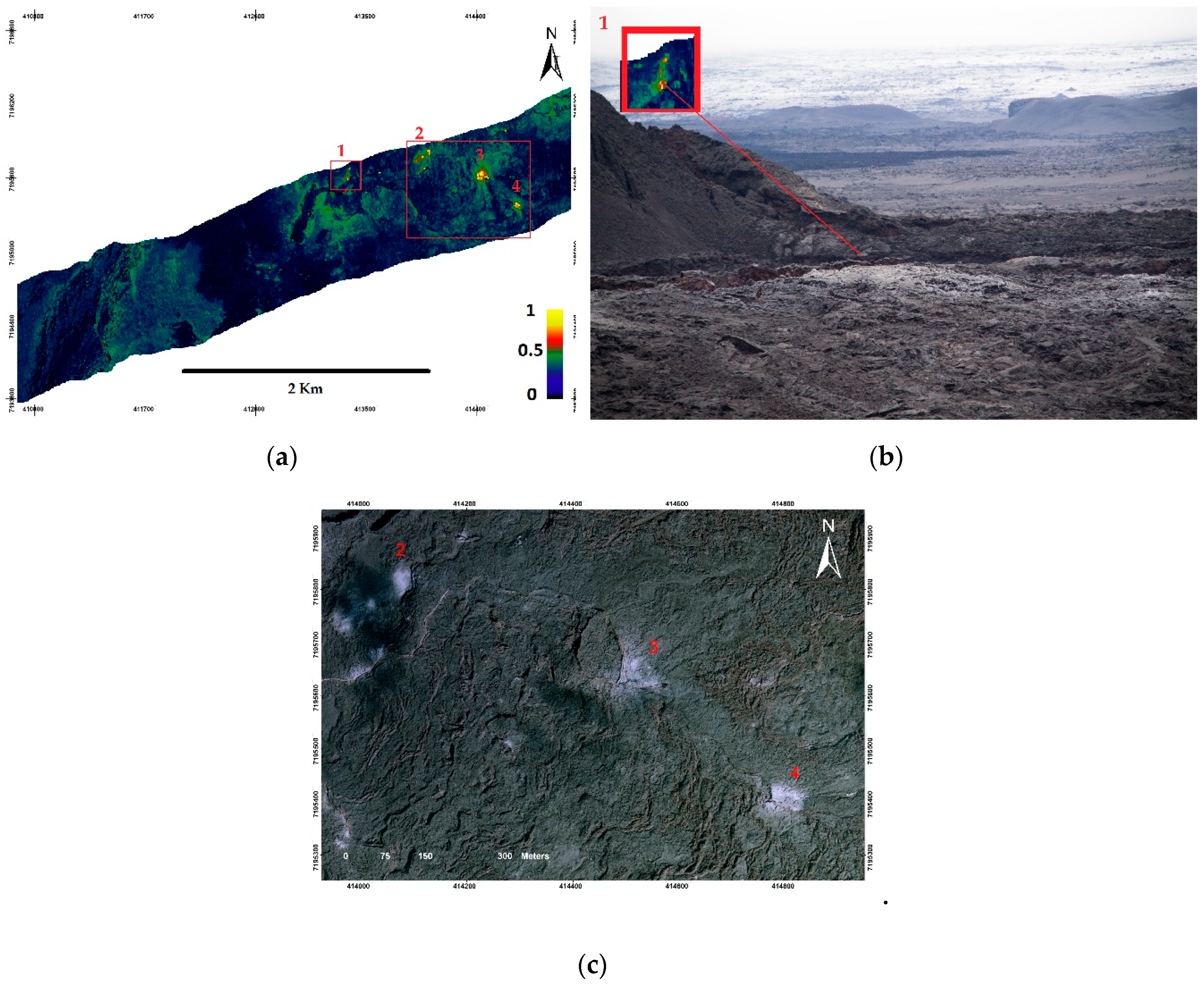
5.3. Hot Material Abundance

As shown in Figure 7a, the hot material abundance map is very sparse. This abundance is described as blends of the endmember 1, 4, 5, and 13 which are characterized by very high reflectance in the SWIR due to the presence of hot material (Figure 5c). Figure 5a shows that endmembers 1, 4, 5, and 13 are located in the lower right corner and the upper part of the image, Figure 7b shows a false color (NIR-SWIR) image which agrees with the abundance map, i.e., some patches of hot material (red-yellow color) exist in the area. The false color image is created by stacking R: 2200 nm; G: 1600 nm, and B: 896 nm. This indicates that the lava field is still emitting hot material during the data acquisition.

5.4. Oxidized Surface Abundance

The oxidized surface endmembers (3, 6, and 12) have the highest abundance fraction at the vent as shown in Figure 8a. This agrees with a field observation shown in Figure 8b which highlights the matching dominant oxidized surface at the vent wall.

5.5. Sulfate Mineral Abundance

The sulfate mineral endmembers (2, 7, 10, 11, and 15) have the highest abundance fraction around the lava pond and there are four most prominent areas for the sulfate (Figure 9a). This surface mineral looked as if it had been dusted by snow (white color) commonly identified as thernadite (Na₂SO₄) [41]. This can be directly seen from a true color image. This mineral formed as the flow cooled, a thin sublimate coating formed on the surface of the lava [41]. Figure 9b,c shows the thernadite formed in surface lava at Holuhraun.

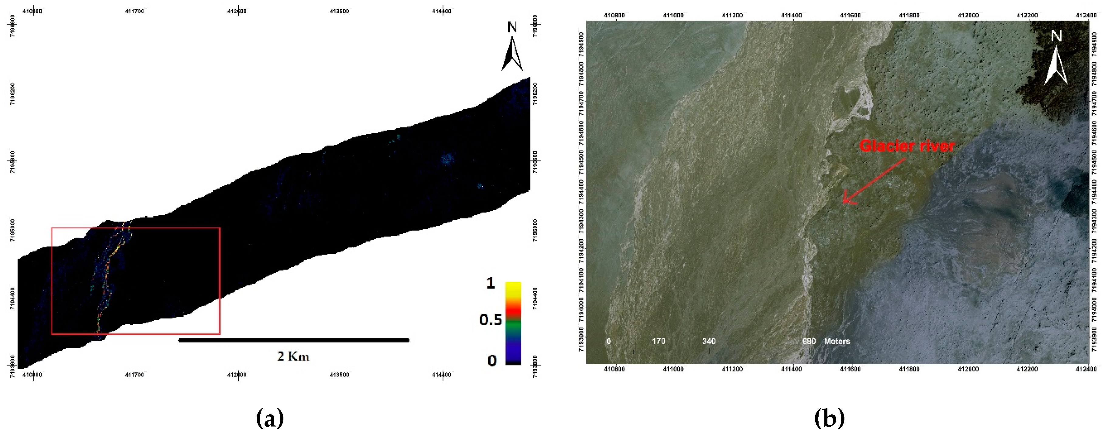
5.6. Water Abundance

The water abundance (Figure 10a) has the highest abundance fraction at the location mainly recognized as a glacial river (Figure 10b). Endmember 14 represents water which is characterized by a relatively low reflectance and has the highest reflectance in the blue wavelength. Water has high absorption and virtually no reflectance in the NIR-SWIR wavelengths range (Figure 5f).

5.7. Noise Abundance

Figure 11 shows the abundance map corresponding to endmember 9. We consider this endmember as representing noise due to an unrecognized spectral signature since this spectrum is characterized by saturated reflectance in channels ~2000 nm and ~2400 nm (Figure 5g). The saturated reflectance could be due to corrupted bands in some pixels.

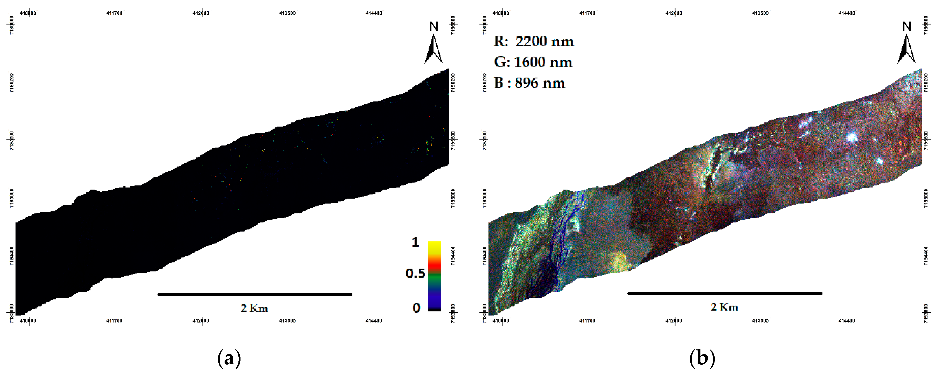
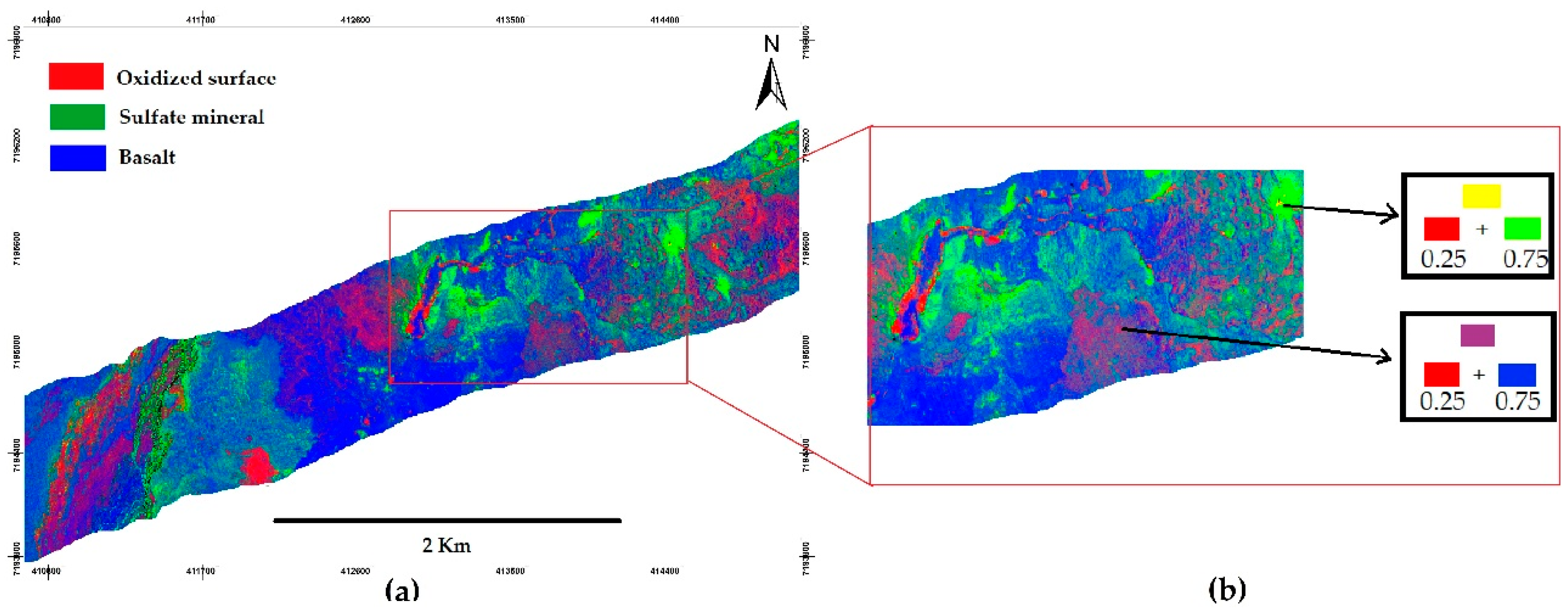
5.8. False Color Abundance

The abundance results depicted as false color (R: Oxidized surface; G: Sulfate mineral; B: Basalt) images show that the majority of rocks or minerals in the study area are dominated by basalt as shown in the blue color in Figure 12a. The other colors such as magenta and yellow indicate a mixture. The mixture phenomenon is illustrated in Figure 12b, as the surface has 0.25 oxidized surface mix with 0.75 basalt resulting in the magenta color; and 0.25 oxidized surface mix with 0.75 sulfate mineral resulting in the yellow color pixel.

5.9. Validation

The very high-resolution aerial photograph was used for ground truth. The aerial photograph was classified into oxidized surface, sulfate, basalt, and water using visual image interpretation and used for validation of the unmixing results. We only validate three endmembers for basalt—oxidized, sulfate, and water—since the noise and hot material cannot be detected based on visual interpretation. We classified the endmembers that have fractional abundance > 0.5. Validation was based on 150 randomly generated point samples within each class.

Table 1. Validation of the endmembers that have abundance > 0.5.

Class	Overall Accuracy	Kappa Index	Mean Overall Accuracy	Mean Kappa Index
Basalt/Non-Basalt	70%	0.62	79%	0.73
Sulfate/Non-Sulfate	93%	0.89
Oxidized/Non-Oxidized	77%	0.72
Water/Non-Water	76%	0.70

show the validation results, with a resulting mean overall accuracy 79% and mean Kappa index of 0.73. This result shows that the abundances have moderate agreement with the sample points.

6. Discussion

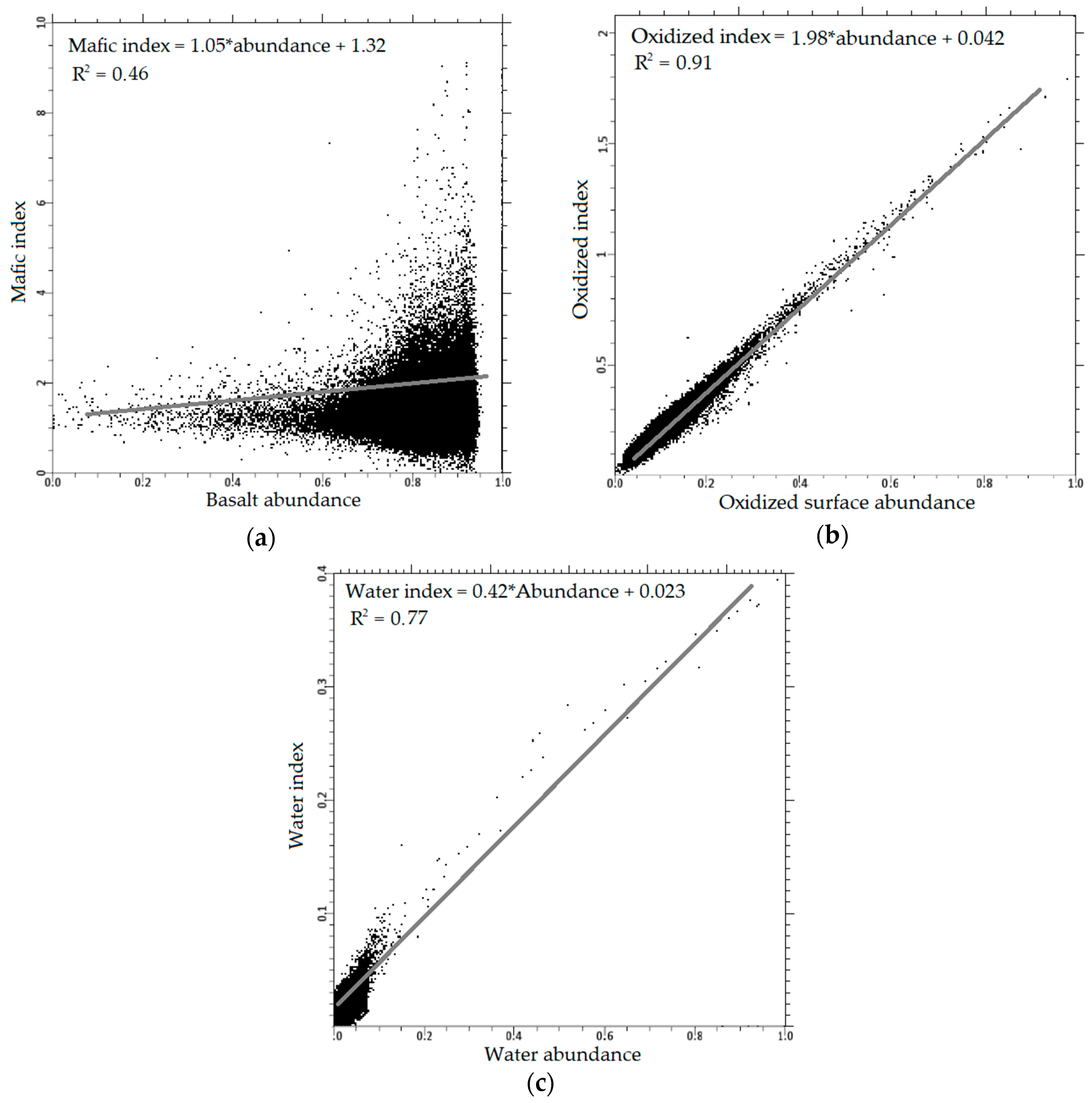
6.1. Comparison with the Existing Spectral Index Technique

The correlation between the spectral index images and the abundance image was analyzed. We only correlated the three endmembers since there are no reference spectral indices for sulfate mineral, hot material, and noise. Here we compared the basalt, oxidized, and water abundance images with the mafic, oxidized, and water index images proposed by Inzana et al., Podwysocki et al. and Xu respectively [42,43,44] (Appendix B). We applied these indices to the hyperspectral image and compared them with the result from each abundance. Figure 13a–c shows the scatter plots results. The R² values were 0.46, 0.91, and 0.77 for the basalt, oxidized surface, and water, respectively. The oxidized surface and water indicate a good correlation with the indices (Figure 13b,c). This suggests that both oxidation and water generated from a spectral index are properly validated [2,44]. Meanwhile, basalt shows a low correlation with the mafic index (Figure 13a) suggesting that the estimates of the basalt surface from the unmixing technique is an overestimation, since the basalt abundance shows the older lava flows as mafic with a relatively high fraction compared to the mafic index that only showed for fresh lava flow. This being due to a full spectrum of hyperspectral can easily differentiate between basalt surface and non-basalt.

6.2. Number of Endmembers

The determination of the number of endmembers is critical, since underestimation may result in a poor representation of the mixed pixels, whereas overestimation may result in an overly segregated area [16].

Table 2. Comparison number of pixels that have abundance >0.5, $\overline{R^2}$ and number of endmembers.

Number of Endmembers	Number of Pixels Abundance						$\overline{R^2}$
	Oxidized Surface	Sulfate Mineral	Hot Material	Water	Noise	Basalt
5	19	57	19	0	0	522481	0.27
10	86	115	19	0	2	522406	0.35
15	91	215	34	373	2	522266	0.71
20	95	232	36	373	5	522046	0.67
30	97	250	40	373	7	521707	0.69

shows the relationship between the number of endmember and the number of pixels that have fractional abundance > 0.5 and the mean correlation with mafic, oxidized, and water index. We considered abundance >0.5 as high abundance. As the number of endmembers increase, the number of pixels also increases for an oxidized surface, sulfate mineral, water, and noise abundances, respectively. This is due to an increase of endmembers that is detected for each group. Meanwhile, the basalt abundance shows the opposite, as the endmembers increase the number of pixels with abundance >0.5 decreases. These results show that as more endmembers are considered the mixing of basalt with other endmembers increases resulting in a decrease of the fractional abundance of basalt. According to the results, we considered the 15 endmembers as an optimum number for this study since they have the highest mean correlation with mafic, oxidized, and water index. Clearly, the selection of appropriate endmembers in such a diverse volcanic environment, considering the particularities of the FENIX dataset, is of great importance in order to obtain accurate unmixing results. In addition, since only a small number of the available materials spectra are expected to be present in a single pixel, the abundance vectors are often sparse [45].

6.3. Size of Lava Field Area

As the methods were only tested on a subset area of the lava field vent, to apply the methods for the entire lava flow is challenging for several reasons. (1) The high spatial heterogeneity typically gives rise to mixed pixels containing multiple materials and it will increase the number of endmembers detected by SMACC [40]. (2) Different illumination occurs within the different flight lines for the entire lava flow (Figure 3b) since the data acquisition time is acquired between 16.56 and 17.58 local times which results from the very low sun angle during the acquisition. This problem can be approached by collecting ground truth spectra, extensive calibration, and atmospheric correction using simultaneous and constrained calibration of multiple hyperspectral images through a new generalized empirical line model purposed by Kizel et al. [37]. (3) The computation time to perform unmixing also must be considered for the entire lava field since the area is relatively large (84 km²) and the hyperspectral data contains 622 channels with a 3.5-meter spatial resolution. In order to process the full set of data we need to consider using high performance computing (HPC) [46].

6.4. Using Full Optical Region for Mapping Recent Lava Flow (VIS-SWIR-TIR)

Hyperspectral VIS-SWIR image data is effective for discrimination mafic, oxidation, sulfate etc. However, not all the minerals and surface type are always mapped uniquely with VIS-SWIR hyperspectral data. A typical surface such as rock forming minerals associated with unaltered rocks and alteration minerals associated with altered rocks can be identified with TIR (Thermal Infrared) data [47,48,49]. Image processing methods that have become standard for hyperspectral VNIR/SWIR data analysis also work for hyperspectral TIR data [47]. Vaughan et al [47] showed that pixel classification techniques based on spectral variability within the scene and mineral libraries for matching spectral emissivity features can be used for TIR-derived mineral maps using SEBASS hyperspectral TIR image data. Hyperspectral TIR instruments operational for airborne surveys are also available in the NERC Airborne Research Facility with a Specim AisaOWL sensor [48]. A synergistic use of airborne data from both FENIX (VIS-SWIR) and OWL (TIR) allows great potential for lava discrimination in future study due to the complementary nature of the reflective (VIS-SWIR) and emissive (TIR) spectral regions. This might significantly improve our understanding of physical lava surface properties. Specifically, VIS-SWIR imaging spectrometers can discriminate surface materials and TIR data acquisitions can help to identify the thermal characteristics of different materials [47,48,49]. For instance, combining emissivity spectra with reflectance spectra in a mixing model would improve discriminating lava from surfaces [50,51,52].

7. Conclusions

In this study, an application of potential spectral unmixing methods on 2014–2015 Holuhraun lava flow field was presented. In total, we acquired fifteen spectral endmembers and their abundances. The first endmember was chosen as the brightest pixel which represented saturated incandescent lava. We grouped these 15 endmembers into six groups (basalt, oxidized surface, sulfate mineral, hot material, water, and noise) based on the shape of the endmembers since the amplitude varies due to illumination conditions, spectral variability, and topography. The endmembers represent pure surface materials in a hyperspectral image. We concluded that the selection of appropriate endmembers in such a diverse volcanic environment, considering the particularities of the FENIX dataset, is of great importance in order to obtain accurate unmixing results. Combination of SMACC and LSMA methods offers an optimum and a fast selection for volcanic products segregation However, ground-truthing spectra are recommended for further analysis. A synergistic use of airborne data from both FENIX (VIS-SWIR) and OWL (TIR) gives a great potential for lava discrimination in future study due to the complementary nature of the reflective (VIS-SWIR) and emissive (TIR) spectral regions. This might significantly improve our understanding of physical lava surface properties.

References

1. Pedersen, G.B.M.; Höskuldsson, A.; Dürig, T.; Thordarson, T.; Jónsdóttir, I.; Riishuus, M.S.; Óskarsson, B.V.; Dumont, S.; Magnusson, E.; Gudmundsson, M.T.; et al. Lava field evolution and emplacement dynamics of the 2014–2015 basaltic fissure eruption at Holuhraun, Iceland. J. Volcanol. Geotherm. Res. 2017. [Google Scholar] [CrossRef]
2. Li, L.; Solana, C.; Canters, F.; Chan, J.; Kervyn, M. Impact of environmental factors on the spectral characteristics of lava surfaces: field spectrometry of basaltic lava flows on Tenerife, Canary Islands, Spain. Remote Sens. 2015, 7, 16986–17012. [Google Scholar] [CrossRef]
3. Li, L.; Solana, C.; Canters, F.; Kervyn, M. Testing random forest classification for identifying lava flows and mapping age groups on a single Landsat 8 image. J. Volcanol. Geotherm. Res. 2017, 345, 109–124. [Google Scholar] [CrossRef]
4. Head, E.M.; Maclean, A.L.; Carn, S.A. Mapping lava flows from Nyamuragira volcano (1967-2011) with satellite data and automated classification methods. Geomatics, Nat. Hazards Risk 2013, 4, 119–144. [Google Scholar] [CrossRef]
5. Li, L.; Canters, F.; Solana, C.; Ma, W.; Chen, L.; Kervyn, M. Discriminating lava flows of different age within Nyamuragira’s volcanic field using spectral mixture analysis. Int. J. Appl. Earth Obs. Geoinf. 2015, 40, 1–10. [Google Scholar] [CrossRef] [Green Version]
6. Amici, S.; Piscini, A.; Neri, M. Reflectance Spectra Measurements of Mt. Etna: A Comparison with Multispectral / Hyperspectral Satellite. Adv. Remote Sens. 2014, 3, 235–245. [Google Scholar] [CrossRef]
7. Graettinger, A.H.; Ellis, M.K.; Skilling, I.P.; Reath, K.; Ramsey, M.S.; Lee, R.J.; Hughes, C.G.; McGarvie, D.W. Remote sensing and geologic mapping of glaciovolcanic deposits in the region surrounding Askja (Dyngjufjöll) volcano, Iceland. Int. J. Remote Sens. 2013, 34, 7178–7198. [Google Scholar] [CrossRef]
8. Zhang, X.; Shang, K.; Cen, Y.; Shuai, T.; Sun, Y. Estimating ecological indicators of karst rocky desertification by linear spectral unmixing method. Int. J. Appl. Earth Obs. Geoinf. 2014, 31, 86–94. [Google Scholar] [CrossRef] [Green Version]
9. Combe, J.P.; Le Mouélic, S.; Sotin, C.; Gendrin, A.; Mustard, J.F.; Le Deit, L.; Launeau, P.; Bibring, J.P.; Gondet, B.; Langevin, Y.; et al. Analysis of OMEGA/Mars Express data hyperspectral data using a Multiple-Endmember Linear Spectral Unmixing Model (MELSUM): Methodology and first results. Planet. Space Sci. 2008, 56, 951–975. [Google Scholar] [CrossRef]
10. Adams, J.B.; Smith, M.O.; Johnson, P.E. Spectral mixture modeling: A new analysis of rock and soil types at the Viking Lander 1 Site. J. Geophys. Res. 1986. [Google Scholar] [CrossRef]
11. Kruse, F.A.; Perry, S.L. Mineral mapping using simulated worldview-3 short-wave-infrared imagery. Remote Sens. 2013, 6, 2688–2703. [Google Scholar] [CrossRef]
12. Sun, Y.; Tian, S.; Di, B. Extracting mineral alteration information using WorldView-3 data. Geosci. Front. 2017. [Google Scholar] [CrossRef]
13. Aufaristama, M.; Höskuldsson, Á.; Jónsdóttir, I.; Ólafsdóttir, R. Mapping and Assessing Surface Morphology of Holocene Lava Field in Krafla ( NE Iceland ) Using Hyperspectral Remote Sensing. IOP Conf. Ser. Earth Environ. Sci. 2016, 29, 1–6. [Google Scholar] [CrossRef]
14. Spinetti, C.; Mazzarini, F.; Casacchia, R.; Colini, L.; Neri, M.; Behncke, B.; Salvatori, R.; Buongiorno, M.F.; Pareschi, M.T. Spectral properties of volcanic materials from hyperspectral field and satellite data compared with LiDAR data at Mt. Etna. Int. J. Appl. Earth Obs. Geoinf. 2009, 11, 142–155. [Google Scholar] [CrossRef]
15. Kolzenburg, S.; Jaenicke, J.; Münzer, U.; Dingwell, D.B. The effect of inflation on the morphology-derived rheological parameters of lava flows and its implications for interpreting remote sensing data - A case study on the 2014/2015 eruption at Holuhraun, Iceland. J. Volcanol. Geotherm. Res. 2018, 357, 200–212. [Google Scholar] [CrossRef]
16. Daskalopoulou, V.; Sykioti, O.; Karagiannopoulou, C. Application of Spectral Unmixing on Hyperspectral data of the Historic volcanic products of Mt. Etna (Italy). Multidiscip. Digit. Publ. Inst. Proc. 2018, 2, 329. [Google Scholar] [CrossRef]
17. Coppola, D.; Ripepe, M.; Laiolo, M.; Cigolini, C. Modelling satellite-derived magma discharge to explain caldera collapse. Geology 2017, 45, 523–526. [Google Scholar] [CrossRef] [Green Version]
18. Aufaristama, M.; Hoskuldsson, A.; Jonsdottir, I.; Ulfarsson, M.; Thordarson, T. New Insights for Detecting and Deriving Thermal Properties of Lava Flow Using Infrared Satellite during 2014–2015 Effusive Eruption at Holuhraun, Iceland. Remote Sens. 2018, 10, 151. [Google Scholar] [CrossRef]
19. Rossi, C.; Minet, C.; Fritz, T.; Eineder, M.; Bamler, R. Temporal monitoring of subglacial volcanoes with TanDEM-X - Application to the 2014-2015 eruption within the Bardarbunga volcanic system, Iceland. Remote Sens. Environ. 2016, 181, 186–197. [Google Scholar] [CrossRef]
20. Dirscherl, M.; Rossi, C. Geomorphometric analysis of the 2014–2015 Bárðarbunga volcanic eruption, Iceland. Remote Sens. Environ. 2018. [Google Scholar] [CrossRef]
21. Adams, J.B.; Sabol, D.E.; Kapos, V.; Almeida Filho, R.; Roberts, D.A.; Smith, M.O.; Gillespie, A.R. Classification of multispectral images based on fractions of endmembers: Application to land-cover change in the Brazilian Amazon. Remote Sens. Environ. 1995. [Google Scholar] [CrossRef]
22. Quintano, C.; Fernández-Manso, A.; Shimabukuro, Y.E.; Pereira, G. Spectral unmixing. Int. J. Remote Sens. 2012. [Google Scholar] [CrossRef]
23. Kolzenburg, S.; Giordano, D.; Thordarson, T.; Höskuldsson, A.; Dingwell, D.B. The rheological evolution of the 2014/2015 eruption at Holuhraun, central Iceland. Bull. Volcanol. 2017, 79, 45. [Google Scholar] [CrossRef]
24. Icelandic Meteorological Office Holuhraun. Available online: http://en.vedur.is/earthquakes-and-volcanism/articles/nr/3122 (accessed on 11 May 2017).
25. Tayebi, M.H.; Tangestani, M.H.; Vincent, R.K.; Neal, D. Spectral properties and ASTER-based alteration mapping of Masahim volcano facies, SE Iran. J. Volcanol. Geotherm. Res. 2014, 287, 40–50. [Google Scholar] [CrossRef]
26. Clark, R.N.; Roush, T.L. Reflectance spectroscopy: quantitative analysis techniques for remote sensing applications. J. Geophys. Res. 1984. [Google Scholar] [CrossRef]
27. Zhang, J.; Rivard, B.; Sánchez-Azofeifa, A. Spectral unmixing of normalized reflectance data for the deconvolution of lichen and rock mixtures. Remote Sens. Environ. 2005. [Google Scholar] [CrossRef]
28. Zhang, J.; Rivard, B.; Sanchez-Azofeifa, A. Derivative spectral unmixing of hyperspectral data applied to mixtures of lichen and rock. IEEE Trans. Geosci. Remote Sens. 2004. [Google Scholar]
29. Rowan, L.C.; Mars, J.C.; Simpson, C.J. Lithologic mapping of the Mordor, NT, Australia ultramafic complex by using the Advanced Spaceborne Thermal Emission and Reflection Radiometer (ASTER). Remote Sens. Environ. 2005. [Google Scholar] [CrossRef]
30. Hellman, M.J.; Ramsey, M.S. Analysis of hot springs and associated deposits in Yellowstone National Park using ASTER and AVIRIS remote sensing. J. Volcanol. Geotherm. Res. 2004. [Google Scholar] [CrossRef]
31. Hyperspectral Imaging Cameras And Systems - Specim. Available online: http://www.specim.fi/ (accessed on 1 December 2018).
32. NERC Airborne Research Facility - British Antarctic Survey. Available online: https://www.bas.ac.uk/polar-operations/sites-and-facilities/facility/nerc-airborne-research-facility-2/ (accessed on 3 December 2018).
33. Loftmyndir ehf. Available online: http://www.loftmyndir.is/ (accessed on 12 February 2019).
34. Bernstein, L.S.; Adler-Golden, S.M.; Sundberg, R.L.; Levine, R.Y.; Perkins, T.C.; Berk, A.; Ratkowski, A.J.; Felde, G.; Hoke, M.L. A new method for atmospheric correction and aerosol optical property retrieval for VIS-SWIR multi- and hyperspectral imaging sensors: QUAC (QUick Atmospheric Correction). IGRSS 2005, 5. [Google Scholar] [CrossRef]
35. Bernstein, L.S. Quick atmospheric correction code: algorithm description and recent upgrades. Opt. Eng. 2012, 51, 111719. [Google Scholar] [CrossRef]
36. Karpouzli, E.; Malthus, T. The empirical line method for the atmospheric correction of IKONOS imagery. Int. J. Remote Sens. 2003. [Google Scholar] [CrossRef]
37. Kizel, F.; Benediktsson, J.A.; Bruzzone, L.; Pedersen, G.B.M.; Vilmundardottir, O.K.; Falco, N. Simultaneous and constrained calibration of multiple hyperspectral images through a new generalized empirical line model. IEEE J. Sel. Top. Appl. Earth Obs. Remote Sens. 2018. [Google Scholar] [CrossRef]
38. Warren, M.A.; Taylor, B.H.; Grant, M.G.; Shutler, J.D. Data processing of remotely sensed airborne hyperspectral data using the Airborne Processing Library (APL): Geocorrection algorithm descriptions and spatial accuracy assessment. Comput. Geosci. 2014, 64, 24–34. [Google Scholar] [CrossRef] [Green Version]
39. Processing/PixelSize. Available online: https://nerc-arf-dan.pml.ac.uk/trac/wiki/Processing/PixelSize (accessed on 31 December 2018).
40. Gruninger, J.H.; Ratkowski, A.J.; Hoke, M.L. The sequential maximum angle convex cone (SMACC) endmember model. SPIE 2004, 5425, 1. [Google Scholar]
41. Moore, R.B.; Clague, D.A.; Rubin, M.; Bohrson, W.A. Volcanism in Hawaii. In U.S. Geological Survey Professional Paper 1350; USGS: Reston, VA, USA, 1987; p. 557. ISBN 3663537137. [Google Scholar]
42. Inzana, J.; Kusky, T.; Higgs, G.; Tucker, R. Supervised classifications of Landsat TM band ratio images and Landsat TM band ratio image with radar for geological interpretations of central Madagascar. J. African Earth Sci. 2003, 37, 59–72. [Google Scholar] [CrossRef]
43. Podwysocki, M.H.; Segal, D.B.; Abrams, M.J. Use of multispectral scanner images for assessment of hydrothermal alteration in the Marysvale, Utah, mining area. Econ. Geol. 1983. [Google Scholar] [CrossRef]
44. Xu, H. Modification of normalised difference water index (NDWI) to enhance open water features in remotely sensed imagery. Int. J. Remote Sens. 2006. [Google Scholar] [CrossRef]
45. Giampouras, P.V.; Themelis, K.E.; Rontogiannis, A.A.; Koutroumbas, K.D. Simultaneously Sparse and Low-Rank Abundance Matrix Estimation for Hyperspectral Image Unmixing. IEEE Trans. Geosci. Remote Sens. 2016. [Google Scholar] [CrossRef]
46. Plaza, A.; Du, Q.; Chang, Y.; King, R.L. High Performance Computing for Hyperspectral Remote Sensing. IEEE J. Sel. Top. Appl. Earth Obs. Remote Sens. 2011, 4, 528–544. [Google Scholar] [CrossRef]
47. Vaughan, R.G.; Calvin, W.M.; Taranik, J.V. SEBASS hyperspectral thermal infrared data: Surface emissivity measurement and mineral mapping. Remote Sens. Environ. 2003, 85, 48–63. [Google Scholar] [CrossRef]
48. Schlerf, M.; Rock, G.; Lagueux, P.; Ronellenfitsch, F.; Gerhards, M.; Hoffmann, L.; Udelhoven, T. A hyperspectral thermal infrared imaging instrument for natural resources applications. Remote Sens. 2012, 4, 3995–4009. [Google Scholar] [CrossRef]
49. Riley, D.; Hecker, C. Mineral Mapping with Airborne Hyperspectral Thermal Infrared Remote Sensing at Cuprite, Nevada, USA. In Thermal Infrared Remote Sensing: Sensors, Methods, Applications; Kuenzer, C., Dech, S., Eds.; Springer: Heidelberg, The Netherlands, 2013; Vol. 17, pp. 495–514. ISBN 978-94-007-6639-6. [Google Scholar]
50. Ball, M.; Pinkerton, H.; Harris, A.J.L. Surface cooling, advection and the development of different surface textures on active lavas on Kilauea, Hawai’i. J. Volcanol. Geotherm. Res. 2008, 173, 148–156. [Google Scholar] [CrossRef]
51. Ramsey, M.S.; Harris, A.J.L.; Crown, D.A. What can thermal infrared remote sensing of terrestrial volcanoes tell us about processes past and present on Mars? J. Volcanol. Geotherm. Res. 2016, 311, 198–216. [Google Scholar] [CrossRef]
52. Harris, A. Thermal Remote Sensing of Active Volcanoes: A User’s Manual; Cambridge University Press: Cambridge, UK, 2013; ISBN 9781139029346. [Google Scholar]
Figure 1. Bárðarbunga volcano and the Holuhraun lava flow field. (a) geological setting by the Icelandic Meteorological Office (after modification) [24], (b) coverage of the three main phases after Pedersen et al [1].
Remotesensing 11 00476 g001
Figure 2. Illustration of (a) the mixed pixel in the lava surface caused by the presence of small, sub pixel targets within the area; (b) variability of lava surfaces in Holuhraun lava field which include the oxidizing surface, sulfate mineral, and lava.
Remotesensing 11 00476 g002
Figure 3. (a) Map showing line acquisition of FENIX hyperspectral image in the Holuhraun lava field; (b) Image mosaic from eight FENIX lines collected during the campaign (red box shows the image subset location); (c) Image subset of the focusing study area in the eruptive fissure vent of Holuhraun.
Remotesensing 11 00476 g003
Figure 4. The workflow processing to derive an abundance map from the FENIX hyperspectral data
Remotesensing 11 00476 g004
Figure 5. (a) The spatial distribution of 15 endmembers extracted by SMACC; The numbers on the image indicate the approximate location of the pixels selected as the represented endmembers of (b) basalt; (c) hot material; (d) oxidized surface; (e) sulfate mineral; (f) water; and (g) noise, extracted by SMACC.
Remotesensing 11 00476 g005
Figure 6. (a) The abundance map for basalt endmember, yellow areas indicate the highest fraction of basalt meanwhile the black areas indicate the lowest fraction of basalt (the red box shows the approximate location of the field photo); (b) field photograph of basaltic lava field of the Holuhraun.
Remotesensing 11 00476 g006
Figure 7. (a) Abundance map for the hot material endmember, yellow areas indicate the highest fraction of hot material meanwhile the black areas indicate the lowest fraction of incandescent lava; (b) The false color (NIR-SWIR) image show that hot material (red-yellow color) exists in the area.
Remotesensing 11 00476 g007
Figure 8. (a) Abundance map oxidized surface endmember; yellow areas indicate the highest fraction of oxidized surface meanwhile the black areas indicate the lowest fraction of oxidized surface; (b) Field photograph of an oxidized surface of the vent wall (red box and the line shows the approximate location of the field photograph)
Remotesensing 11 00476 g008
Figure 9. (a) The Abundance map for the sulfate mineral endmember, the yellow areas indicate the highest fraction of sulfate mineral meanwhile the black areas indicate the lowest fraction of the sulfate mineral; (b) Field photograph of sulfate mineral (white surface) formed on the surface of lava (the red boxes and lines show the approximate location of the field and aerial photo respectively); (c) aerial photograph of sulfate mineral (white surface) formed on the surface of lava (The numbers on the image indicate the approximate location of the sulfate for both the abundance and photograph).
Remotesensing 11 00476 g009
Figure 10. (a) The abundance map for water endmember, the highest abundance fraction indicated by a yellow color, and the lowest abundance fraction indicated by a black red box shows the approximate location of the aerial photograph); (b) aerial photograph of the glacial river.
Remotesensing 11 00476 g010
Figure 11. The abundance map for the noise endmember, the highest abundance fraction is indicated by the yellow color, and the lowest abundance fraction is indicated by the black color.
Remotesensing 11 00476 g011
Figure 12. (a) False color of abundance highlighting for R: oxidized surface; G: sulfate mineral; and B: Basalt; (b) Illustration of the mixed pixels in the area, 0.25 oxidized surface mix with 0.75 basalt resulting in the magenta color; and 0.25 oxidized surface mix with 0.75 sulfate mineral resulting in the yellow color pixel.
Remotesensing 11 00476 g012
Figure 13. Linear regression analysis between the spectral index images and the (a) basalt abundance; (b) oxidized surface abundance; and (c) water index.
Remotesensing 11 00476 g013