Adversarial Reconstruction-Classification Networks for PolSAR Image Classification

Abstract

Polarimetric synthetic aperture radar (PolSAR) image classification has become more and more widely used in recent years. It is well known that PolSAR image classification is a dense prediction problem. The recently proposed fully convolutional networks (FCN) model, which is very good at dealing with the dense prediction problem, has great potential in resolving the task of PolSAR image classification. Nevertheless, for FCN, there are some problems to solve in PolSAR image classification. Fortunately, Li et al. proposed the sliding window fully convolutional networks (SFCN) model to tackle the problems of FCN in PolSAR image classification. However, only when the labeled training sample is sufficient, can SFCN achieve good classification results. To address the above mentioned problem, we propose adversarial reconstruction-classification networks (ARCN), which is based on SFCN and introduces reconstruction-classification networks (RCN) and adversarial training. The merit of our method is threefold: (i) A single composite representation that encodes information for supervised image classification and unsupervised image reconstruction can be constructed; (ii) By introducing adversarial training, the higher-order inconsistencies between the true image and reconstructed image can be detected and revised. Our method can achieve impressive performance in PolSAR image classification with fewer labeled training samples. We have validated its performance by comparing it against several state-of-the-art methods. Experimental results obtained by classifying three PolSAR images demonstrate the efficiency of the proposed method.

1. Introduction

Polarimetric synthetic aperture (PolSAR) image classification is one of the most prominent applications in geoscience remote sensing [1]. Over the last few years, substantial amount of PolSAR image data has been put into use [2]. Consequently, PolSAR image classification has gained significant research attention [3,4] and many methods to accomplish this task came into existence [4,5]. The majority of the available methods are based on physical scattering mechanisms, which are obtained through various polarimetric decomposition methods [6]. Polarimetric target decomposition is one of the most powerful and widely used methods for PolSAR image classification. The physical characteristics corresponding to the target are used to describe the architecture in the polarimetric target decomposition theorem. Several polarimetric target decomposition methods are reported in the literature. To name a few, they are Krogager decomposition [7], Cloude-Pottier decomposition [8], Pauli decomposition [9], Huynen decomposition [10], Freeman decomposition [11], and the extensions of the above mentioned decomposition methods [12,13]. Besides, some researchers believed that the statistical distribution of PolSAR data can be used for classifying the PolSAR images [14,15]. For instance, derived from the complex Wishart distributions of the covariance and coherency matrices, Lee et al. [15,16] used Wishart distance to accomplish the task of the PolSAR image classification. In addition, the research on PolInSAR technique has also received a lot of attention [17,18,19,20,21]. However, all these methods mentioned above are highly depend on a complex analysis of PolSAR data [22], and the extensive analysis of the physical mechanism is hard [23].

In addition, with the advancements seen in computing technology, machine learning-based methods became crucial for PolSAR image classification. Plethora of image classification techniques based on k-nearest neighbor (KNN) [24], support vector machine (SVM) [25,26,27], Bayes [28], sparse representation [23,29], neural networks [30,31,32] and stacked auto-encoder (SAE) [33] etc. are available in the literature. Previously, many researchers have successfully used such methods for PolSAR image classification and have obtained satisfactory results.

In recent years, the convolutional neural network (CNN) model, derived from convolution, pool and nonlinear transformation operations, has obtained good results in many applications [34,35], i.e., action recognition [36], semantic segmentation [37], image classification [38] and scene labeling [39]. Nonetheless, the existing CNN model are not suitable for PolSAR image classification. It is well known that PolSAR image classification task is dense prediction problem. For the existing CNN’s classification framework, input is image and output is class of image. Nevertheless, CNN’s classification result cannot describe the image detail [40]. Consequently, for the existing CNN’s classification frameworks for PolSAR image [41,42,43], pixel’s neighborhood is set as the input image. In this way, the pixel’s class can be obtained. In other words, CNN has no advantage in memory occupation. Luckily, Long et al. proposed fully convolutional networks (FCN) model [40], which can be trained in an end-to-end, pixels-to-pixels manner. FCN converts fully connected layers of traditional CNN model into convolutional layers. By this means, an efficient classification net for end-to-end dense learning can be enabled. Accordingly, FCN has great potential in processing PolSAR image classification task. Nevertheless, because each PolSAR image has a different size, FCN cannot be directly applied to PolSAR image classification. Consequently, the existing FCN frameworks does not have a specific framework capable of processing all PolSAR images. Larger size input image also increases the complexity of the classification framework. Recently, Li et al. [44] proposed sliding window fully convolutional networks (SFCN) to tackle the problems of FCN in PolSAR image classification. The sliding window operation of SFCN is similar to that of CNN, and Li et al. [44] have designed a new training framework for SFCN. Nevertheless, because of the relatively complex network architecture of SFCN, it cannot obtain excellent classification results with fewer labeled training samples.

Based on deep learning, Ghifary et al. [45] presented a new model called deep reconstruction- classification network (DRCN) for object recognition. DRCN can jointly learn a shard feature representation for two tasks: (i) supervised source data classification; and (ii) unsupervised target data reconstruction. In this way, the extracted feature representation can preserve discriminability while encoding meaningful information from the target data. Similar to the standard neural networks, DRCN can also be optimized by backpropagation. DRCN has obtained considerable improvement over the state-of-the-art methods in cross-domain object recognition task.

Adversarial training has become the state-of-the-art method for generative image modeling. Luc et al. [46] proposed an adversarial training method which is very helpful for training segmentation models. In their approach, a convolutional segmentation network with an adversarial network is trained to discriminate the segmentation maps coming either from the segmentation network or the ground truth. Their method can detect and revise the higher-order inconsistencies between the ground truth maps and segmentation result maps.

Based on the SFCN, DRCN and adversarial training models, we propose adversarial reconstruction-classification networks (ARCN) in this paper. The merits of our method can be expressed as: (i) Since our method is based on SFCN, it can be trained end-to-end, pixels-to-pixels while taking into account the spatial information; (ii) Our method can jointly learn a shard feature representation for supervised image classification and unsupervised image reconstruction. In this way, all samples can be correctly classified, not just labeled training samples; (iii) By introducing adversarial training, our method can enforce forms of higher-order consistency between the true image and reconstructed image. The rest of this paper is organized as follows. The methods used to extract features for PolSAR images are given in Section 2. Section 3 describes the related work. Our proposed ARCN method is shown in Section 4. Section 5 reports the experimental results. Finally, discussion and conclusions are provided in Section 6 and Section 7.

2. Feature Extraction of PolSAR Images

2.1. Coherency Matrix

On the basis of [22], PolSAR data can be expressed with scattering matrix, which is given by Equation (1). In addition, PolSAR data’s polarimetric information is contained in scattering matrix.

$$\mathit{S}=\left[\begin{array}{cc}{S}_{hh}& S_{hv}\\ S_{vh}& S_{vv}\end{array}\right].$$

(1)

In the case of the monostatic backscattering, there exists the reciprocity theorem, i.e., $S_{hv}$ = $S_{vh}$. The scattering matrix can also be expressed as: [47]:

$$\mathit{S}=a\frac{1}{\sqrt{2}}\left[\begin{array}{cc}1& 0\\ 0& 1\end{array}\right]+b\frac{1}{\sqrt{2}}\left[\begin{array}{cc}1& 0\\ \hfill 0& -1\end{array}\right]+c\frac{1}{\sqrt{2}}\left[\begin{array}{cc}0& 1\\ 1& 0\end{array}\right],$$

(2)

where

$$a=(S_{hh}+S_{vv})/\sqrt{2},b=(S_{hh}-S_{vv})/\sqrt{2},c=\sqrt{2}{S}_{hv}.$$

(3)

In addition, PolSAR data’s coherency matrix $\mathit{T}$ can be expressed as follows [22]:

$$\mathit{T}={[a,b,c]}^T[a^{*},b^{*},c^{*}]=\left[\begin{array}{ccc}{T}_{11}& T_{12}& T_{13}\\ T_{21}& T_{22}& T_{23}\\ T_{31}& T_{32}& T_{33}\end{array}\right]=\left[\begin{array}{ccc}\hfill {\left|a\right|}^2& a{b}^{*}& a{c}^{*}\\ a^{*}b& {\left|b\right|}^2& b{c}^{*}\\ a^{*}c& b^{*}c& {\left|c\right|}^2\end{array}\right].$$

(4)

In recent years, many great performances corresponding to PolSAR image classification have been obtained by the coherency matrix $\mathit{T}$ [22,23].

2.2. Cloude-Pottier Decomposition

As described in the eigen-decomposition model [8], coherence matrix T is decomposed as:

$$\mathit{T}={\mathit{U}}_3\left[\begin{array}{ccc}{\lambda }_1& 0& 0\\ 0& {\lambda }_2& 0\\ 0& 0& {\lambda }_3\end{array}\right]{\mathit{U}}_3^{*}=\sum _{i=1}^3{\lambda }_i{\overrightarrow{e}}_i{\overrightarrow{e}}_i^{*},$$

(5)

where ${\mathit{U}}_3=[{\overrightarrow{e}}_1,{\overrightarrow{e}}_2,{\overrightarrow{e}}_3]$ and ${\lambda }_i(i=1,2,3)$ are eigenvector matrix and eigenvalue of $\mathit{T}$, respectively. According to the eigen-decomposition model, Cloude and Pottier put forward Cloude-Pottier decomposition model. The entropy H, the anisotropy A, and the mean alpha angle $\overline{\alpha }$ are defined as:

$$\begin{array}{c}H=-\sum _{i=1}^3{p}_{i}lo{g}_3{p}_i,p_i=\frac{{\lambda }_i}{{\sum }_{k=1}^3{\lambda }_k},\\ A=\frac{{\lambda }_2-{\lambda }_3}{{\lambda }_2+{\lambda }_3},\\ \overline{\alpha }=\sum _{i=1}^3{p}_i{\alpha }_i=p_{1}co{s}^{-1}(e_1^1)+p_{2}co{s}^{-1}(e_2^1)+p_{3}co{s}^{-1}(e_3^1),\end{array}$$

(6)

where $e_i^1$ (i = 1, 2, 3) is the first element of ${\overrightarrow{e}}_i$ (i = 1, 2, 3). Besides, Cloude-Pottier decomposition model plays an important role in processing PolSAR image classification task [6,8].

The features we extract in this paper are divided into two parts, $\mathit{F}$ = [${\mathit{F}}_1$, ${\mathit{F}}_2$]. To construct the first part of $\mathit{F}$, i.e., ${\mathit{F}}_1$, we use the coherency matrix T; ${\mathit{F}}_1$ = [$T_{11}$, $T_{22}$, $T_{33}$, Re($T_{12}$), Re($T_{13}$), Re($T_{23}$)]. Here, Re($T_{ij}$) and Im($T_{ij}$) represent the real and the imaginary parts of $T_{ij}$, respectively. Now, by making use of the Cloude-Pottier decomposition features, we construct the second part of the features as ${\mathit{F}}_2$ = [H, A, $\overline{\alpha }$, ${\lambda }_1$, ${\lambda }_2$, ${\lambda }_3$].

3. Related Work

3.1. Sliding Window Fully Convolutional Networks

FCN is a natural extension of CNN to solve the dense prediction problem, for example image segmentation. To recover the resolution information corresponding to the input at the output layer, upsampling layers are added to the standard architectures by FCN. Therefore, images of arbitrary size can be processed with FCN. FCN uses skip connections between the upsampling and downsampling paths to tackle the resolution problem caused by downsampling operation. Skip connections are very helpful for the upsampling path to recover the fine-grained information from the downsampling layers. However, as Section 1 described, FCN cannot be directly applied in PolSAR image classification. Images of different sizes need different FCN frameworks and larger-size input images generally increase the difficulty in designing network architecture. Therefore, we cannot design a corresponding framework for each PolSAR image alone. To design a unified FCN architecture for different PolSAR images, Li et al. introduced sliding window operator in [44]. The sliding window operation of SFCN is similar to that of CNN, and the number of the images obtained by sliding window operation can be acquired through

$$\mathit{num}=(ceil((Height-W)/S)+1)·(ceil((Width-W)/S)+1),$$

(7)

where ceil denotes the upward integer-valued function, Height and width respectively denote the height and width of the image, W and S respectively denote the size and stride of the sliding window operation, and $\mathit{num}$ denotes the number of the acquired images obtained by sliding window operation.

3.2. Deep Reconstruction-Classification Networks

DRCN jointly learns two tasks: (i) supervised classification of the source data, and (ii) unsupervised reconstruction of the target data. The two tasks share the encoding parameters, while the decoding parameters of the two tasks are separated. DRCN’s core contribution is to construct a single composite feature representation, which encodes information for both the classification task of the source data and the structure of the target data. The purpose is that the learned supervised classification function can obtain good classification results in the target data. That is to say, the unsupervised reconstruction task can be regarded as the auxiliary task to support the adaption of the classification task.

3.3. Semantic Segmentation Using Adversarial Networks

In [46], Luc et al. use an adversarial training method to increase the performance of segmentation model. Their method more interested in forcing higher-order consistency than a very specific class of high-order potentials. Motivated by the generative adversarial network (GAN) model [48], they find a method through adversarial training rather than searching to directly integrate higher-order potentials in a conditional random field (CRF) model. For this reason, their objective function is consisted of a conventional multi-class cross-entropy loss and an adversarial term. The adversarial term encourages semantic segmentation model to generate result maps, which cannot be distinguished from the ground truth maps with an adversarial classification network. Because the adversarial network can evaluate the joint configuration of multiple label variables, it can force forms of higher-order consistency.

4. Methodology

In this paper, we propose a novel PolSAR image classification method, which we refer to as adversarial reconstruction-classification networks (ARCN). We first present the architecture of reconstruction-classification networks (RCN), which based on the SFCN model. Then, we give the architecture and training details of our proposed ARCN method.

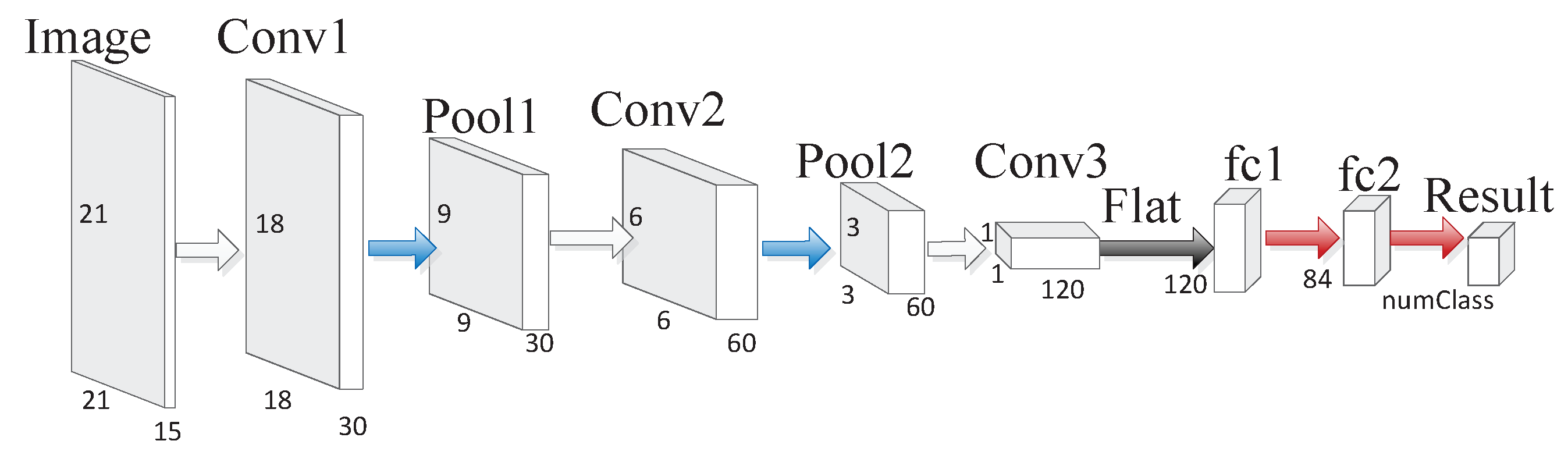
4.1. Reconstruction-Classification Networks

RCN consists of two pipelines: (i) supervised classification network, and (ii) unsupervised reconstruction network, which can be shown in Figure 1. In addition, the classification network part of Figure 2 gives the framework of SFCN. The two pipelines can be divided into three functions: (i) encoding function, which can be expressed by the intersection between the red rectangle and blue rectangle in Figure 1; (ii) classification function, which can be expressed by the rest part of the red rectangle in Figure 1; (iii) reconstruction function, which can be expressed by the rest part of the blue rectangle in Figure 1. That is to say, RCN has two pipelines with a shared encoding representation. The RCN model is optimized through multitask learning [49], namely, jointly learns the supervised classification and unsupervised reconstruction tasks. The purpose is that the encoding function can learn the commonality between the two tasks. In this way, excellent classification results still can be obtained when the number of the labeled training samples is limited.

We now describe RCN more formally. Let $f_c$: $\mathcal{X}\to {\mathcal{Y}}_c$ be the supervised image classification pipeline and $f_r$: $\mathcal{X}\to \mathcal{X}$ be the unsupervised reconstruction image pipeline of RCN, where $\mathcal{X}$ and ${\mathcal{Y}}_c$ represent the input image space and the ground truth space, respectively. Define the three functions mentioned above: (i) encoding function $g_{enc}$: $\mathcal{X}\to \mathcal{F}$, (ii) reconstruction function $g_{rec}$: $\mathcal{F}\to \mathcal{X}$, and (iii) classification function $g_{cla}$: $\mathcal{F}\to {\mathcal{Y}}_c$, where $\mathcal{F}$ represents the encoding feature space. Given an input image x ∈$\mathcal{X}$, $f_c$ and $f_r$ can be described as follow:

$$\begin{array}{c}{f}_c(x)=(g_{cla}\circ g_{enc})(x),\end{array}$$

(8)

$$\begin{array}{c}{f}_r(x)=(g_{rec}\circ g_{enc})(x).\end{array}$$

(9)

Let ${\mathsf{\Theta }}_c$ = {${\mathsf{\Theta }}_{enc}$, ${\mathsf{\Theta }}_{cla}$} and ${\mathsf{\Theta }}_r$ = {${\mathsf{\Theta }}_{enc}$, ${\mathsf{\Theta }}_{rec}$} respectively represent the parameters of the supervised classification model and unsupervised reconstruction model. ${\mathsf{\Theta }}_{enc}$, ${\mathsf{\Theta }}_{rec}$, and ${\mathsf{\Theta }}_{cla}$ are the parameters of the encoding, reconstruction, and classification functions, respectively. The aim is to find a shared encoding function $g_{enc}$ which supports both $f_c$ and $f_r$.

As for the unsupervised reconstruction model, we use adversarial training to train it, which is described next.

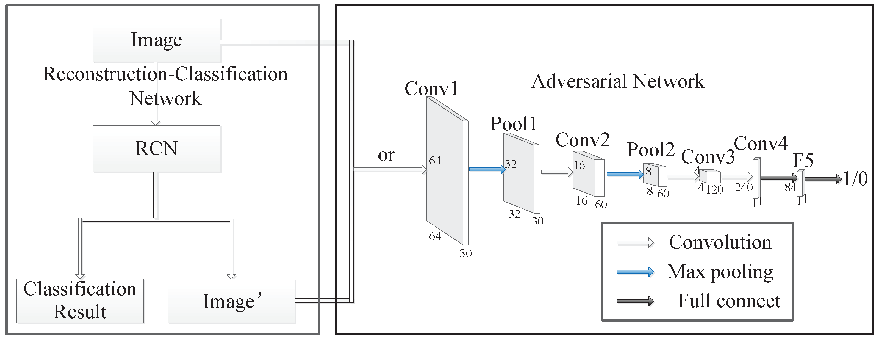
4.2. Adversarial Reconstruction-Classification Networks

4.2.1. Adversarial Training for RCN

ARCN can be divided into two parts: RCN and adversarial networks, which can be shown in Figure 2. The left black rectangle in Figure 2 represents the RCN model, which takes Image as input and produces the classification result and the reconstruction of the Image. Meanwhile, the right black rectangle takes image map as input and produces class label (1 = true image, or 0 = synthetic).

Let ${\mathsf{\Theta }}_a$ represents the parameters of the adversarial networks, and $f_a$: $\mathcal{X}\to {\mathcal{Y}}_d$ be the adversarial networks, where ${\mathcal{Y}}_d\in$ [0, 1]. Given an input image x ∈$\mathcal{X}$, $f_a$ can be expressed as follow:

$$f_a(X)=\left\{\begin{array}{c}1,X=x\hfill \\ 0,X=f_r(x)\hfill \end{array}\right.$$

(10)

Given $N_1$ labeled training samples ($x_i,y_i$), where $y_i\in {\{0,1\}}^K$ is a one-hot vector, and $N_2$ unlabeled training samples $x_j$, the loss can be defined as:

$${\mathcal{L}}_{ARCN}({\mathsf{\Theta }}_c,{\mathsf{\Theta }}_r,{\mathsf{\Theta }}_a)=\sum _{i=1}^{N_1}{l}_c(f_c(x_i),y_i)-\lambda l_a(f_a(f_r(x_i)),0)-\lambda [\sum _{i=1}^{N_1}{l}_a(f_a(x_i),1)+\sum _{j=1}^{N_2}{l}_a(f_a(x_j),1)+l_a(f_a(f_r(x_j)),0)].$$

(11)

In the above, $l_c(\widehat{y},y)=-{\sum }_{k=1}^K{y}_{k}ln{\widehat{y}}_k$ represents the multi-class cross-entropy loss for predictions $\widehat{y}$, which is the softmax output. Similarly, we use $l_a(\widehat{z},z)=-[zln\widehat{z}+(1-z)ln(1-\widehat{z})]$, the binary cross-entropy loss. We minimize the loss with respect to the parameters ${\mathsf{\Theta }}_c$ and ${\mathsf{\Theta }}_r$ of RCN, while maximizing the loss with respect to the parameters ${\mathsf{\Theta }}_a$ of the adversarial networks.

4.2.2. Training the Adversarial Model

Since only the terms in Equation (11) that contain $l_a$ depend on the adversarial networks, the loss of the adversarial model can be described as:

$$\begin{array}{c}{\mathcal{L}}_A({\mathsf{\Theta }}_a)=\sum _{i=1}^{N_1}{l}_a(f_a(f_r(x_i)),0)+l_a(f_a(x_i),1)+\sum _{j=1}^{N_2}{l}_a(f_a(f_r(x_i)),0)+l_a(f_a(x_j),1).\end{array}$$

(12)

The training of the adversarial model minimizes the above loss function, and the architectures of our adversarial model can be shown by the right black rectangle in Figure 2.

4.2.3. Training the RCN Model

Given the adversarial networks, training the RCN model is equivalent to minimize the multi-class cross-entropy loss, while decreasing the performance of the adversarial networks. In this way, it is not easy for the adversarial model to distinguish the reconstructed image produced by the RCN model from the true image. The objective function corresponding to the RCN model can be described as follow:

$$\begin{array}{c}{\mathcal{L}}_{RCN}({\mathsf{\Theta }}_c,{\mathsf{\Theta }}_r)=\sum _{j=1}^{N_2}-\lambda l_a(f_a(f_r(x_j)),0)+\sum _{i=1}^{N_1}{l}_c(f_c(x_i),y_i)-\lambda l_a(f_a(f_r(x_i)),0).\end{array}$$

(13)

Similar to Goodfellow et al. [48], we replace the term $-\lambda l_a(f_a(f_r(x)),0)$ with $\lambda l_a(f_a(f_r(x)),1)$. That is to say, we maximize the probability that the adversarial model predicts $f_r(x)$ to be the true image instead of minimizing the probability that the adversarial model predicts it to be the synthetic image. It is not difficult to prove that $-\lambda l_a(f_a(f_r(x)),0)$ with $\lambda l_a(f_a(f_r(x)),1)$ have the same set of critical points. The reason of this update is that it produces a stronger gradient signal when the adversarial model makes an accurate prediction of the true/synthetic image. It has been proven by the preliminary experiments that this update is very meaningful for accelerating training process [46]. Therefore, the objective function of the RCN model can be updated to follow:

$$\begin{array}{c}{\mathcal{L}}_{RCN}({\mathsf{\Theta }}_c,{\mathsf{\Theta }}_r)=\sum _{j=1}^{N_2}\lambda l_a(f_a(f_r(x_j)),1)+\sum _{i=1}^{N_1}{l}_c(f_c(x_i),y_i)+\lambda l_a(f_a(f_r(x_i)),1).\end{array}$$

(14)

The optimization of ${\mathcal{L}}_{ARCN}$ can be obtained by alternately minimizing ${\mathcal{L}}_A$ and ${\mathcal{L}}_{RCN}$ using ADAM [50]. We will count the training classification accuracy for each iteration. The algorithm will stop in two cases. First, the training classification accuracy of multiple consecutive iterations is higher than the predefined accuracy value. Second, the iteration number reaches the predefined maximum iteration number. Our proposed ARCN method is summarized in Algorithm 1. In addition, we use dropout regularization [51] during the minimization of ${\mathcal{L}}_{RCN}$ to prevent overfitting.

Algorithm 1 The adversarial reconstruction-classificati networks (ARCN) learning algorithm.

Input: Labeled samples: ${\{(x_i,y_i)\}}_{i=1}^{N_1}$; Unlabeled samples ${\{x_j\}}_{j=1}^{N_2}$; Learning rate: ${\alpha }_c,{\alpha }_r,{\alpha }_a$;

1: Initialize parameters ${\mathsf{\Theta }}_c,{\mathsf{\Theta }}_r,{\mathsf{\Theta }}_a$; 2: while not stop do 3:   for each labeled samples batch do 4:   Do a forward pass according to Equations (8)–(10); 5:   Update ${\mathsf{\Theta }}_c,{\mathsf{\Theta }}_r,{\mathsf{\Theta }}_a$: $$\begin{array}{c}{\mathsf{\Theta }}_c\leftarrow {\mathsf{\Theta }}_c-{\alpha }_c{\mathsf{\nabla }}_{{\mathsf{\Theta }}_c}{\mathcal{L}}_{RCN}({\mathsf{\Theta }}_c);\\ {\mathsf{\Theta }}_r\leftarrow {\mathsf{\Theta }}_r-{\alpha }_r{\mathsf{\nabla }}_{{\mathsf{\Theta }}_r}{\mathcal{L}}_{RCN}({\mathsf{\Theta }}_r);\\ {\mathsf{\Theta }}_a\leftarrow {\mathsf{\Theta }}_a-{\alpha }_a{\mathsf{\nabla }}_{{\mathsf{\Theta }}_a}{\mathcal{L}}_A({\mathsf{\Theta }}_a);\end{array}$$ 6:   end for 7:   for each unlabeled samples batch do 8:   Do a forward pass according to Equations (9)–(10);   9:   Update ${\mathsf{\Theta }}_r,{\mathsf{\Theta }}_a$: $$\begin{array}{c}{\mathsf{\Theta }}_r\leftarrow {\mathsf{\Theta }}_r-{\alpha }_r{\mathsf{\nabla }}_{{\mathsf{\Theta }}_r}{\mathcal{L}}_{RCN}({\mathsf{\Theta }}_r);\\ {\mathsf{\Theta }}_a\leftarrow {\mathsf{\Theta }}_a-{\alpha }_a{\mathsf{\nabla }}_{{\mathsf{\Theta }}_a}{\mathcal{L}}_A({\mathsf{\Theta }}_a);\end{array}$$ 10:   end for 11: end while

Output: ARCN learnt parameters: $\widehat{\mathsf{\Theta }}$ = $\{{\widehat{\mathsf{\Theta }}}_c,{\widehat{\mathsf{\Theta }}}_r,{\widehat{\mathsf{\Theta }}}_a\}$.

5. Experimental Results

As previously stated in Section 2, in this work, we use coherency matrix T and Cloude-Pottier decomposition features as our extracted original features. The feature dimension is 15. As a matter of pre-processing, we have used a refined Lee filter [52] to reduce speckle noise. To validate the performance of our proposed method, we have used the following three PolSAR images: Xi’an, China; Oberpfaffenhofen, Germany; San Francisco, USA. The performance of the proposed method is compared against SVM [26], sparse representation classifier (SRC) [53], SAE [33], CNN [54], and SFCN [44]. Overall accuracy (OA) and Kappa coefficients [55] are used as evaluation criteria. All methods are implemented in a 3.20-GHz machine with a 8.00-GB RAM and a NVIDIA GTX 1050 Ti GPU.

5.1. Description of Experimental PolSAR Images

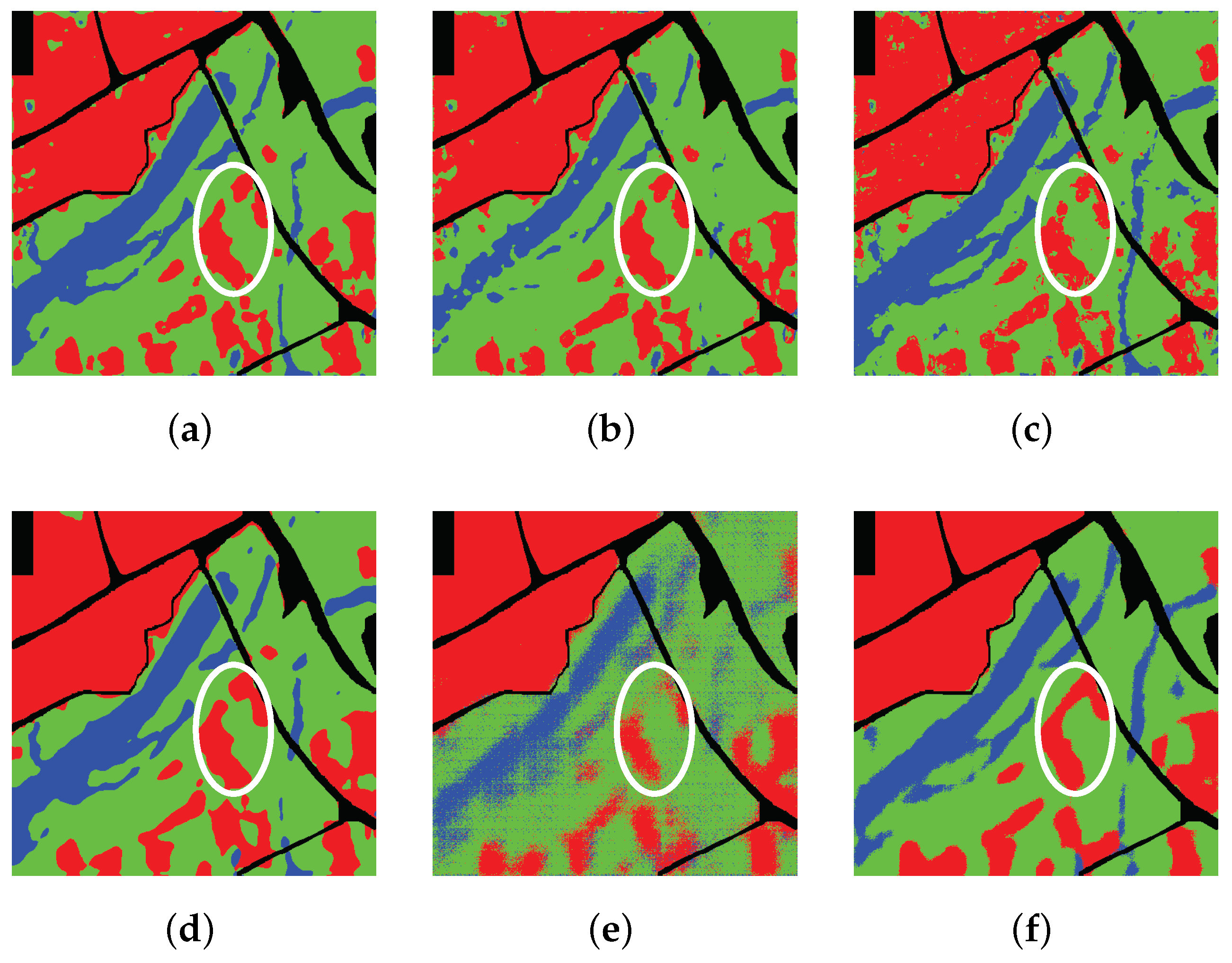
5.1.1. Xi’an

The first PolSAR iamge is acquired from a C-band multilook PolSAR image, which covers western Xi’an, Shaanxi, China. The left of Figure 3a gives its PauliRGB image with its corresponding coordinate, and the size of which is 512 × 512. The right of Figure 3a gives the photo of the near area of Xi’an, which is from Google Maps. The corresponding ground truth map is shown in Figure 3b, which is acquired by referencing [56]. Overall, 237,416 pixels are labeled in Figure 3b. Xi’an image mainly contains 3 classes, which are water, grass and building. The corresponding code map is shown in Figure 3c.

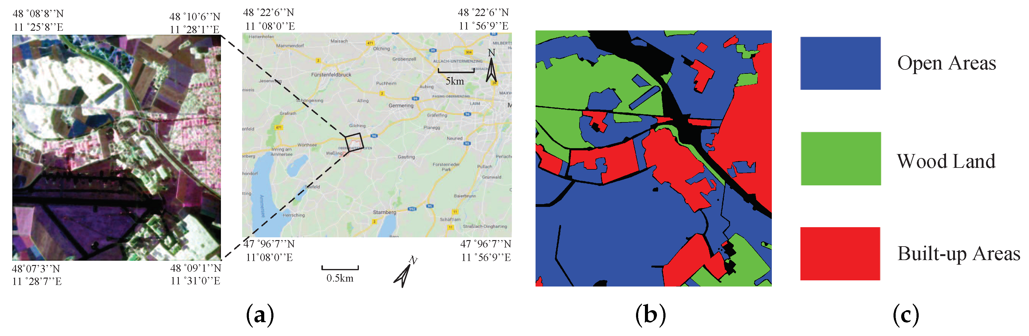
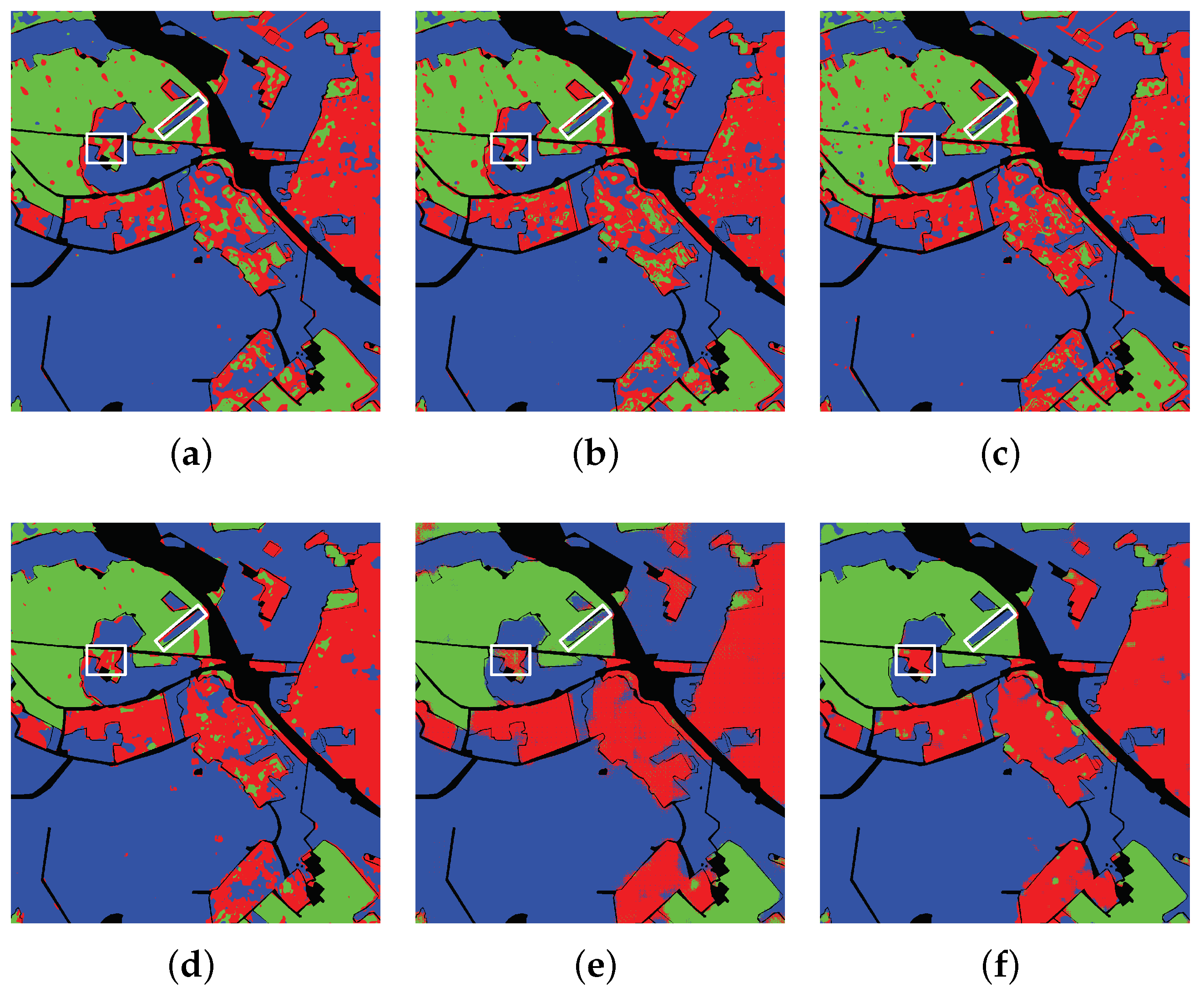
5.1.2. Oberpfaffenhofen

The second PolSAR image is acquired from an L-band multilook PolSAR image, which covers Oberpfaffenhofen, Germany. German Aerospace Center’s E-SAR provided this PolSAR image. The size of this PolSAR image is 1300 × 1200, which is shown in the left of Figure 4a. The right of Figure 4 gives the photo of the near area of Oberpfaffenhofen, which is from Google Maps. The ground truth is shown in Figure 4b, which is obtained by referencing [43]. In total there are 1,374,298 labeled pixels. The corresponding ground truth map is shown in Figure 4c. From the ground truth map, we can see that there are three classes in this PolSAR image: open areas, wood land and built-up areas.

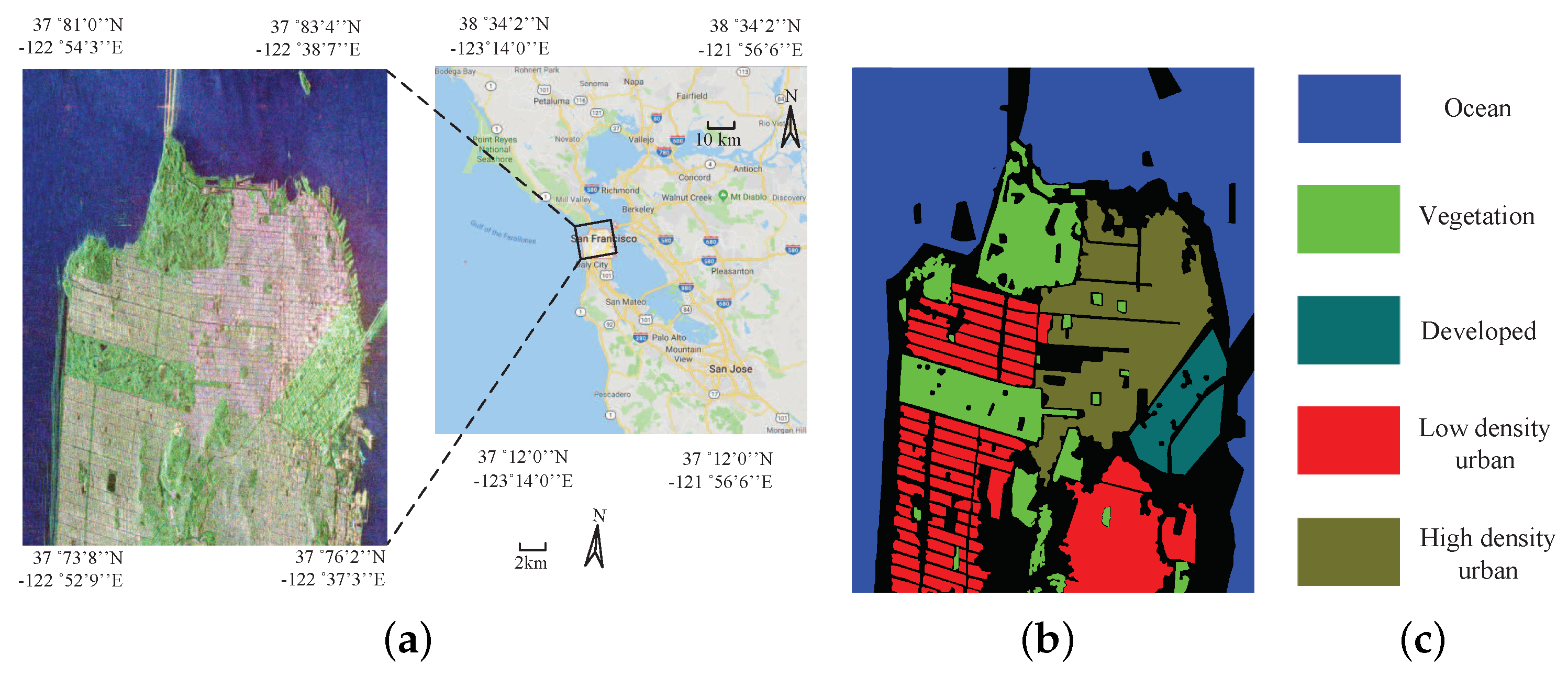
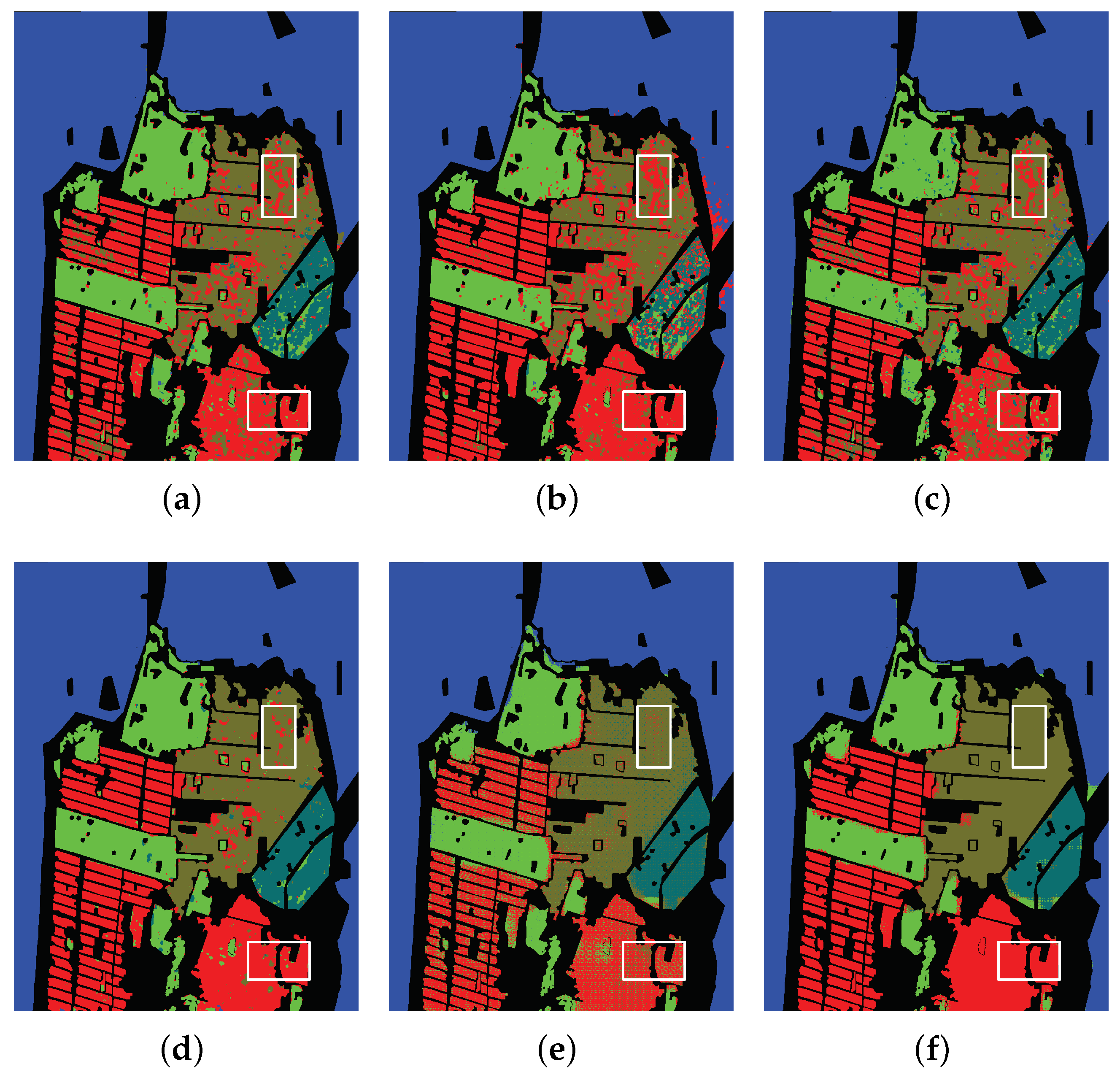
5.1.3. San Francisco

The third PolSAR image is gained from a C-band multilook PolSAR image, which covers the area around the bay of San Francisco with the golden gate bridge. Because this PolSAR image provides a good coverage of both natural terrain and man-made terrain, it has been widely used in PolSAR image classification. The size of this PolSAR image is 1800 × 1380, which is shown in the left of Figure 5a. The right of Figure 5a gives the photo of the near area of San Francisco, which is from Google Maps. Figure 5b gives the corresponding ground truth map, which is acquired by referencing [43]. The number of the labeled pixels is 1,804,087. This data set mainly contains five classes: ocean, vegetation, developed, low density urban and high density urban, and the corresponding color code is shown in Figure 5c.

5.2. Parameter Setting

As for the SVM method, the radial basis function (RBF) kernel is used. For the SRC method, we set the number of dictionary atoms to 15. For the SAE model, the dimensions of middle layers are fixed to 300 and 100, respectively. A $21\times 21$ neighborhood is used for each pixel with the CNN model, and Figure 6 gives the classification architecture of CNN. The sliding window size and stride in Equation (7) are fixed to 128 and 64, respectively. For the SFCN model, it has the same architecture as that of the classification network of RCN model. Figure 1 and Figure 2 show our method’s architecture. Next, for all experiments, the rate of training samples used for each class for the three PolSAR images are 1%, 0.2% and 0.1%, respectively. For SFCN and our proposed method, only the training pixels are involved in modifying the network parameters in the training stage.

5.3. Classification Performance

5.3.1. Xi’an Data Set

As previously stated, 1% of the labeled pixels are used for training and the rest are used for testing. The classification accuracy of our method and three compared method are shown in

Table 1. Classification results of Xi’an with various methods.

Methods	Water	Grass	Building	OA	Kappa
SVM	0.8167	0.9075	0.9012	0.8916	0.8199
SRC	0.5754	0.9169	0.9031	0.8607	0.7624
SAE	0.8861	0.8736	0.8957	0.8833	0.8086
CNN	0.8159	0.8990	0.9382	0.9004	0.8352
SFCN	0.5833	0.8437	0.8957	0.8229	0.7059
ARCN	0.8074	0.9527	0.9540	0.9313	0.8856

. From Table 1, we can see that our method has better classification accuracy, which is about 3.97%, 7.06%, 4.80%, 3.09% and 10.84% higher than that of the five compared methods, respectively.

The classification results of Xi’an with various methods are shown in Figure 7. As shown in Figure 7a–c, the results of SVM, SRC and SAE are not well in regional continuity. For example, the building in the upper left corner is misclassified to grass. From Figure 7d, we can see that CNN does not perform well in the marginal areas of classes. It is because CNN use a $21\times 21$ neighborhood of each pixel as the input image, which increases the difficulty of classifying the pixels in the above mentioned areas. As for SFCN, it does not perform well in recognizing water, which is shown in Figure 7e. Because the selected training samples are too few, SFCN cannot learn the internal structure of Xi’an. On the other hand, as can be seen in Figure 7f, our method has clearly outperformed the compared methods, with fewer misclassified pixels. Furthermore, we use white ellipse to highlight the notable different classification results. From the white ellipse, it can be seen that the building is classified better with our method than five compared methods. In summary, the effectiveness of our method can be proven.

5.3.2. Oberpfaffenhofen Data Set

Out of the labeled pixels, 0.2% are used for training and the rest for testing. The classification accuracy on Oberpfaffenhofen obtained with our method and compared methods is listed in

Table 2. Classification results of oberpfaffenhofen with various methods.

Methods	Built-up Areas	Wood Land	Open Areas	OA	Kappa
SVM	0.6978	0.8665	0.9682	0.8815	0.7959
SRC	0.7237	0.8380	0.9498	0.8721	0.7809
SAE	0.7807	0.8284	0.9604	0.8902	0.8119
CNN	0.8266	0.9234	0.9677	0.9242	0.8704
SFCN	0.9220	0.9157	0.9588	0.9413	0.9006
ARCN	0.9173	0.9551	0.9837	0.9617	0.9348

. From the classification results in Table 2, we can see that the OA of our method is about 8.02%, 8.96%, 7.15%, 3.75% and 2.04% higher than that of the five compared methods, respectively.

Figure 8 shows the classification result of Oberpfaffenhofen with different methods. As to SVM, SRC and SAE, there are a large number of misclassified pixels for all classes, which can be seen in Figure 8a–c. For CNN, we can see many misclassified pixels between open areas and built-up areas in Figure 8d. From Figure 8e, we can see that the classification result of SFCN is desirable. However, SFCN does not perform well in the edge parts of classes. As shown in Figure 8f, our method obtains better classification result than the methods used for comparison. Simultaneously, the remarkable different classification results are highlighted by the white rectangles in Figure 8. The visual comparison of classification results corresponding to the white rectangles shows that large amount of pixels are misclassified by the five compared methods. For the noted above, the effectiveness of our proposed ARCN method can be demonstrated.

5.3.3. San Francisco Data Set

In this case, we use 0.1% of the labeled pixels for training and the remaining for testing.

Table 3. Classification results of San Francisco with various methods.

Methods	Ocean	Vegetation	Low Density Urban	High Density Urban	Developed	OA	Kappa
SVM	0.9983	0.9146	0.8720	0.7735	0.8163	0.9193	0.8837
SRC	0.9890	0.8830	0.9457	0.7093	0.5142	0.9016	0.8576
SAE	0.9990	0.8978	0.8334	0.7841	0.8583	0.9135	0.8754
CNN	0.9999	0.9611	0.9754	0.9156	0.9514	0.9747	0.9635
SFCN	0.9998	0.9016	0.8273	0.9325	0.8046	0.9340	0.9051
ARCN	0.9977	0.8817	0.9962	0.9873	0.9238	0.9772	0.9672

lists the classification accuracy on San Francisco computed by the six aforementioned methods. From Table 3, we can see that our method has higher classification accuracy than the five compared methods. Nevertheless, the gap between the OA of CNN and our method is not large.

Figure 9 shows the classification result of San Francisco with the aforementioned four methods. As shown in Figure 9a–c, the classification results of SVM, SRC and SAE are relatively worse. From Figure 9d, we can see that the classification result of CNN is well in regional continuity. Because the structure of San Francisco is not complicated, for example, water itself occupies a large area, where does not contain other classes. Furthermore, CNN can take into account the spatial information, which facilitates the image classification. From Figure 9e, we can see that the classification result of SFCN is acceptable. Furthermore, we use white rectangles to highlight the remarkable different classification results in Figure 9. Through comparing the classification results of white rectangles, it can be concluded that our method acquire a better classification result than the five compared methods. In summary, all these results clearly demonstrate the efficiency of our proposed ARCN method in classifying San Francisco.

6. Discussion

6.1. Accuracy

As mentioned in Section 5.2, the amount of training samples used with the three images are 1%, 0.2% and 0.1%, i.e., 2375, 2751 and 1807 of labeled pixels. From our study we see that the number of selected samples with our method is much less than that of the available state-of-the-art methods [22,33]. Nevertheless, our method still manages to obtain comparatively better results. We strongly believe that this is due to the following reasons: (i) Because our method is based on SFCN, an efficient classification net for end-to-end dense learning can be learned; (ii) Our method can jointly learn a shared encoding representation for two tasks: supervised image classification and unsupervised image reconstruction. By optimizing unsupervised image reconstruction task, the learnt encoding representation is highly abstract, which facilitates the image classification task. Since the learnt encoding representation can be used to reconstruct all the samples and classify the labeled training samples, the rest samples, which belong to the same distribution as the labeled training samples, can also be classified correctly with the learnt encoding representation; (iii) By introducing adversarial training, our method can enforce forms of higher-order consistency between the truth image and reconstructed image. For these reasons, our method can obtain excellent classification results with a small number of labeled training samples.

6.2. Execution Time

Table 4. Execution time of the three PolSAR Images with different methods (S).

Methods	Xi’an			Oberpfaffenhofen			San Francisco
	Train	Predict	Total	Train	Predict	Total	Train	Predict	Total
SVM	0.07	5.13	5.20	0.12	62.52	62.64	0.03	44.48	44.51
SRC	0.49	0.40	0.89	0.34	2.24	2.58	0.27	2.70	2.97
SAE	7.93	0.21	8.14	8.97	0.58	9.55	5.97	1.08	7.05
CNN	41.26	3.02	44.28	33.1	18.94	52.04	35.1	30.66	65.76
SFCN	24.89	0.11	25.00	30.49	0.73	31.22	36.38	1.29	37.67
ARCN	206.57	0.11	206.68	286.72	0.74	287.46	195.05	1.29	196.34

summarizes the execution time of various methods corresponding to three PolSAR images, where “Train” denotes the training time, "Predict" denotes the time taken to classify entire image, and “Total” denotes the total time used to train plus predict. From Table 4, we can see that the execution time of our method is higher than that of the methods used for comparison. The reasons for this can be stated as follows: (i) Our method requires to process two tasks simultaneously, i.e., supervised image classification and unsupervised image reconstruction; (ii) Our method introduces adversarial training, which is time consuming.

6.3. Memory Consumption

The memory consumption of various methods corresponding to three PolSAR images is given in

Table 5. Memory consumption of various methods corresponding to three PolSAR Images (G).

Methods	Xi’an	Oberpfaffenhofen	San Francisco
SVM	0.026	0.14	0.24
SRC	0.026	0.14	0.24
SAE	0.026	0.14	0.24
CNN	11.9	66.1	110.5
SFCN	0.076	0.55	0.85
ARCN	0.076	0.55	0.85

, and the symbol “G” in the caption of Table 5 denotes gigabytes. From Table 5, we can see that the memory consumption of CNN is the highest among all the methods. The main reason is that for the classification framework of CNN used in PolSAR images, the neighborhood of the pixel is set as the input to get the class of the pixel. Compared with CNN, the memory consumption of the rest two compared methods and our method is satisfied. black

In summary, SVM, SRC and SAE cannot obtain satisfactory results in PolSAR image classification, because they donot take the spatial information of the image into consideration. Nevertheless, they perform very well in time consumption and memory occupation except that the predict time of SVM is relatively longer than other two methods. CNN can take into account the spatial information by setting the neighborhood of the pixel as the input image. Consequently, CNN capable of obtaining acceptable classification result. However, setting the neighborhood of the pixel as the input image of the CNN model also results in repeated memory consumption, which causes the shortcoming of CNN in memory consumption. Because the framework of SFCN is more complex than that of CNN and SAE, so SFCN needs more labeled training samples to get promising classification results. Therefore, SFCN does not get ideal classification results in this paper. For our proposed ARCN method, it can jointly learn a shared feature representation for supervised image classification and unsupervised image reconstruction while introducing adversarial learning. Therefore, our method can get competitive classification results with fewer labeled training samples. Furthermore, our method also performs well in memory consumption. However, our method still has room for improvement in terms of time consumption.

7. Conclusions

This paper presents a novel classification method, namely ARCN, for PolSAR image classification. We set the coherency matrix T and Cloude-Pottier decomposition features as the original feature vectors. In this paper, we have compared our method’s performance against SVM, SRC, SAE, CNN, and SFCN on classifying three PolSAR images (Xi’an, Oberpfaffenhofen, and San Francisco). The recently proposed SFCN model can be trained end-to-end, pixels-to-pixels while taking the spatial information into consideration. Nevertheless, only when the training sample is sufficient can SFCN get good classification results. To address the above mentioned problem, RCN and adversarial training are introduced to our method. A shared feature representation can be jointly learned by RCN for supervised image classification and unsupervised image reconstruction, and the higher-order inconsistencies between the true image and reconstructed image can be detected and revised by adversarial training. In this way, our method can achieve impressive performance in PolSAR image classification with fewer labeled training samples. In addition, our method has a relatively longer training phase. Our future work is concentrated on finding a method to reduce the time consumed in the training stage for our method.

References

1. Chen, W.; Gou, S.; Wang, X.; Li, X.; Jiao, L. Classification of PolSAR Images Using Multilayer Autoencoders and a Self-Paced Learning Approach. Remote Sens. 2018, 10, 110. [Google Scholar] [CrossRef]
2. Zhang, F.; Ni, J.; Yin, Q.; Li, W.; Li, Z.; Liu, Y.; Hong, W. Nearest-Regularized Subspace Classification for PolSAR Imagery Using Polarimetric Feature Vector and Spatial Information. Remote Sens. 2017, 9, 1114. [Google Scholar] [CrossRef]
3. Hou, B.; Chen, C.; Liu, X.; Jiao, L. Multilevel distribution coding model-based dictionary learning for PolSAR image classification. IEEE J. Sel. Top. Appl. Earth Obs. 2015, 8, 5262–5280. [Google Scholar]
4. Cheng, J.; Ji, Y.; Liu, H. Segmentation-based PolSAR image classification using visual features: RHLBP and color features. Remote Sens. 2015, 7, 6079–6106. [Google Scholar] [CrossRef]
5. Tao, C.; Chen, S.; Li, Y.; Xiao, S. PolSAR land cover classification based on roll-invariant and selected hidden polarimetric features in the rotation domain. Remote Sens. 2017, 9, 660. [Google Scholar]
6. Zhang, L.; Sun, L.; Zou, B.; Moon, W.M. Fully Polarimetric SAR Image Classification via Sparse Representation and Polarimetric Features. IEEE J. Sel. Top. Appl. Earth Obs. 2015, 8, 3923–3932. [Google Scholar] [CrossRef]
7. Krogager, E. New decomposition of the radar target scattering matrix. Electron. Lett. 1990, 26, 1525–1527. [Google Scholar] [CrossRef]
8. Cloude, S.R.; Pottier, E. An entropy based classification scheme for land applications of polarimetric SAR. IEEE Trans. Geosci. Remote Sens. 1997, 35, 68–78. [Google Scholar] [CrossRef]
9. Xu, Q.; Chen, Q.; Yang, S.; Liu, X. Superpixel-based classification using K distribution and spatial context for polarimetric SAR images. Remote Sens. 2016, 8, 619. [Google Scholar] [CrossRef]
10. Huynen, J.R. Phenomenological theory of radar targets. Electromagn. Scatt. 1978, 653–712. [Google Scholar] [CrossRef]
11. Freeman, A.; Durden, S.L. A three-component scattering model for polarimetric SAR data. IEEE Trans. Geosci. Remote Sens. 1998, 36, 963–973. [Google Scholar] [CrossRef]
12. Van Zyl, J.J.; Arii, M.; Kim, Y. Model-based decomposition of polarimetric SAR covariance matrices constrained for nonnegative eigenvalues. IEEE Trans. Geosci. Remote Sens. 2011, 49, 3452–3459. [Google Scholar] [CrossRef]
13. Yamaguchi, Y.; Moriyama, T.; Ishido, M.; Yamada, H. Four-component scattering model for polarimetric SAR image decomposition. IEEE Trans. Geosci. Remote Sens. 2005, 43, 1699–1706. [Google Scholar] [CrossRef]
14. Kong, J.A.; Swartz, A.A.; Yueh, H.A.; Novak, L.M.; Shin, R.T. Identification of terrain cover using the optimum polarimetric classifier. J. Electromagn. Waves Appl. 1988, 2, 171–194. [Google Scholar]
15. Lee, J.-S.; Grunes, M.R.; Kwok, R. Classification of multi-look polarimetric SAR imagery based on complex Wishart distribution. Int. J. Remote Sens. 1994, 15, 2299–2311. [Google Scholar] [CrossRef]
16. Lee, J.-S.; Grunes, M.R.; Ainsworth, T.L.; Du, L.-J.; Schuler, D.-L.; Cloude, S.R. Unsupervised classification using polarimetric decomposition and the complex Wishart classifier. IEEE Trans. Geosci. Remote Sens. 1999, 37, 2249–2258. [Google Scholar]
17. Schneider, R.Z.; Papathanassiou, K.P.; Hajnsek, I.; Moreira, A. Polarimetric and interferometric characterization of coherent scatterers in urban areas. IEEE Trans. Geosci. Remote Sens. 2006, 44, 971–984. [Google Scholar] [CrossRef]
18. Shimoni, M.; Borghys, D.; Heremans, R.; Perneel, C.; Acheroy, M. Fusion of PolSAR and PolInSAR data for land cover classification. Int. J. Appl. Earth Obs. 2009, 11, 169–180. [Google Scholar] [CrossRef]
19. Garestier, F.; Dubois-Fernandez, P.; Dupuis, X.; Paillou, P.; Hajnsek, I. PolInSAR analysis of X-band data over vegetated and urban areas. IEEE Trans. Geosci. Remote Sens. 2006, 44, 356–364. [Google Scholar] [CrossRef]
20. Biondi, F. Multi-chromatic analysis polarimetric interferometric synthetic aperture radar (MCA-PolInSAR) for urban classification. Int. J. Remote Sens. 2018, 1–30. [Google Scholar] [CrossRef]
21. Chen, S.; Wang, X.; Sato, M. PolInSAR complex coherence estimation based on covariance matrix similarity test. IEEE Trans. Geosci. Remote Sens. 2012, 50, 4699–4710. [Google Scholar] [CrossRef]
22. Liu, F.; Jiao, L.; Hou, B.; Yang, S. POL-SAR Image classification based on Wishart DBN and local spatia information. IEEE Trans. Geosci. Remote Sens. 2016, 54, 3292–3308. [Google Scholar] [CrossRef]
23. Chen, Y.; Jiao, L.; Li, Y.; Zhao, J. Multilayer Projective Dictionary Pair Learning and Sparse Autoencoder for PolSAR Image Classification. IEEE Trans. Geosci. Remote Sens. 2017, 55, 6683–6694. [Google Scholar] [CrossRef]
24. Richardson, A.; Goodenough, D.G.; Chen, H.; Moa, B.; Hobart, G.; Myrvold, W. Unsupervised nonparametric classification of polarimetric SAR data using the K-nearest neighbor graph. In Proceedings of the IEEE International Geoscience and Remote Sensing Symposium (IGARSS), Honolulu, HI, USA, 25–30 July 2010; pp. 1867–1870. [Google Scholar]
25. Zhang, L.; Zou, B.; Zhang, J.; Zhang, Y. Classification of polarimetric SAR image based on support vector machine using multiple-component scattering model and texture features. EURASIP J. Adv. Signal Process. 2010, 2010. [Google Scholar] [CrossRef]
26. Lardeux, C.; Frison, P.L.; Tison, C.C.; Souyris, J.C.; Stoll, B.; Fruneau, B.; Rudant, J.P. Support vector machine for multifrequency SAR polarimetric data classification. IEEE Trans. Geosci. Remote Sens. 2009, 47, 4143–4152. [Google Scholar] [CrossRef]
27. Fukuda, S.; Hirosawa, H. Support vector machine classification of land cover: application to polarimetric SAR data. In Proceedings of the IEEE International Geoscience and Remote Sensing Symposium (IGARSS), Sydney, Australia, 9–13 July 2001; pp. 187–189. [Google Scholar]
28. Yueh, H.A.; Swartz, A.A.; Kong, J.A.; Shin, R.T.; Novak, L.M. Bayes classification of terrain cover using normalized polarimetric data. J. Geophys. Res. 1988, 93, 15261–15267. [Google Scholar] [CrossRef]
29. Chen, Y.; Jiao, L.; Li, Y.; Li, L.; Zhang, D.; Ren, B.; Marturi, N. A Novel Semicoupled Projective Dictionary Pair Learning Method for PolSAR Image Classification. IEEE Trans. Geosci. Remote Sens. 2018. [Google Scholar] [CrossRef]
30. Chen, K.-S.; Huang, W.; Tsay, D.; Amar, F. Classification of multifrequency polarimetric SAR imagery using a dynamic learning neural network. IEEE Trans. Geosci. Remote Sens. 1996, 34, 814–820. [Google Scholar] [CrossRef]
31. Hellmann, M.; Jager, G.; Kratzschmar, E.; Habermeyer, M. Classification of full polarimetric SAR-data using artificial neural networks and fuzzy algorithms. In Proceedings of the IEEE International Geoscience and Remote Sensing Symposium (IGARSS), Hamburg, Gemany, 28 June–2 July 1999; pp. 1995–1997. [Google Scholar]
32. Chen, C.; Chen, K.; Lee, J. The use of fully polarimetric information for the fuzzy neural classification of SAR images. IEEE Trans. Geosci. Remote Sens. 2003, 41, 2089–2100. [Google Scholar] [CrossRef]
33. Hou, B.; Kou, H.; Jiao, L. Classification of Polarimetric SAR Images Using Multilayer Autoencoders and Superpixels. IEEE J. Sel. Top. Appl. Earth Obs. 2016, 9, 3072–3081. [Google Scholar] [CrossRef]
34. Voulodimos, A.; Doulamis, N.; Doulamis, A.; Protopapadakis, E. Deep learning for computer vision: A brief review. Comput. Intell. Neurosci. 2018, 2018, 1–13. [Google Scholar] [CrossRef]
35. Zhang, L.; Zhang, L.; Du, B. Deep learning for remote sensing data: A technical tutorial on the state of the art. IEEE Geosci. Remote Sens. Mag. 2016, 4, 22–40. [Google Scholar] [CrossRef]
36. Simonyan, K.; Zisserman, A. Two-stream convolutional networks for action recognition in videos. In Proceedings of the Conference on Advances in Neural Information Processing Systems (NIPS), Montreal, QC, Canada, 8–13 December 2014; pp. 568–576. [Google Scholar]
37. Girshick, R.; Donahue, J.; Darrell, T.; Malik, J. Rich feature hierarchies for accurate object detection and semantic segmentation. In Proceedings of the IEEE Conference on Computer Vision and Pattern Recognition (CVPR), Columbus, OH, USA, 23–28 June 2014; pp. 580–587. [Google Scholar]
38. Krizhevsky, A.; Sutskever, I.; Hinton, G.E. Imagenet classification with deep convolutional neural networks. In Proceedings of the International Conference on Neural Information Processing Systems (NIPS), Lake Tahoe, NV, USA, 3–6 December 2012; pp. 1097–1105. [Google Scholar]
39. Farabet, C.; Couprie, C.; Najman, L.; LeCun, Y. Learning hierarchical features for scene labeling. IEEE Trans. Pattern Anal. Mach. Intell. 2013, 35, 1915–1929. [Google Scholar] [CrossRef] [PubMed]
40. Long, J.; Shelhamer, E.; Darrell, T. Fully convolutional networks for semantic segmentation. In Proceedings of the IEEE Conference on Computer Vision and Pattern Recognition (CVPR), Boston, MA, USA, 7–12 June 2015; pp. 3431–3440. [Google Scholar]
41. Zhu, X.; Tuia, D.; Mou, L.; Xia, G.; Zhang, L.; Xu, F.; Fraundorfer, F. Deep Learning in Remote Sensing: A Comprehensive Review and List of Resources. IEEE Geosci. Remote Sens. Mag. 2017, 5, 8–36. [Google Scholar] [CrossRef] [Green Version]
42. Zhou, Y.; Wang, H.; Xu, F.; Jin, Y. Polarimetric SAR image classification using deep convolutional neural networks. IEEE Geosci. Remote Sens. Lett. 2016, 13, 1935–1939. [Google Scholar] [CrossRef]
43. Xie, W.; Jiao, L.; Hou, B.; Ma, W.; Zhao, J.; Zhang, S.; Liu, F. POLSAR image classification via Wishart-AE model or Wishart-CAE model. IEEE J. Sel. Top. Appl. Earth Obs. 2017, 10, 3604–3615. [Google Scholar] [CrossRef]
44. Li, Y.; Chen, Y.; Liu, G.; Jiao, L. A Novel Deep Fully Convolutional Network for PolSAR Image Classification. Remote Sens. 2018, 10, 1984. [Google Scholar] [CrossRef]
45. Ghifary, M.; Kleijn, W.B.; Zhang, M.; Balduzzi, D.; Li, W. Deep reconstruction-classification networks for unsupervised domain adaptation. In Proceedings of the European Conference on Computer Vision (ECCV), Amsterdam, The Netherlands, 8–16 October 2016; pp. 597–613. [Google Scholar]
46. Luc, P.; Couprie, C.; Chintala, S.; Verbeek, J. Semantic segmentation using adversarial networks. arXiv, 2016; arXiv:1611.08408. [Google Scholar]
47. Cloude, S.R.; Pottier, E. A review of target decomposition theorems in radar polarimetry. IEEE Trans. Geosci. Remote Sens. 1996, 34, 498–518. [Google Scholar] [CrossRef]
48. Goodfellow, I.; Pouget-Abadie, J.; Mirza, M.; Xu, B.; Warde-Farley, D.; Ozair, S.; Courville, A.; Bengio, Y. Generative adversarial nets. In Proceedings of the Conference on Advances in Neural Information Processing Systems (NIPS), Montreal, QC, Canada, 8–13 December 2014; pp. 2672–2680. [Google Scholar]
49. Caruana, R. Multitask learning. Mach. Learn. 1997, 28, 41–75. [Google Scholar] [CrossRef]
50. Kingma, D.P.; Ba, J. Adam: A Method for Stochastic Optimization. In Proceedings of the International Conference on Learning Representations (ICLR), San Diego, CA, USA, 7–9 May 2015. [Google Scholar]
51. Srivastava, N.; Hinton, G.; Krizhevsky, A.; Sutskever, I.; Salakhutdinov, R. Dropout: A simple way to prevent neural networks from overfitting. J. Mach. Learn. Res. 2014, 15, 1929–1958. [Google Scholar]
52. Lee, J.-S.; Grunes, M.R.; De Grandi, G. Polarimetric SAR speckle filtering and its implication for classification. IEEE Trans. Geosci. Remote Sens. 1999, 37, 2363–2373. [Google Scholar]
53. Gu, S.; Zhang, L.; Zuo, W.; Feng, X. Projective dictionary pair learning for pattern classification. In Proceedings of the Conference on Advances in Neural Information Processing Systems (NIPS), Montreal, QC, Canada, 8–13 December 2014; pp. 793–801. [Google Scholar]
54. Ding, J.; Chen, B.; Liu, H.; Huang, M. Convolutional neural network with data augmentation for SAR target recognition. IEEE Geosci. Remote Sens. Lett. 2016, 13, 364–368. [Google Scholar] [CrossRef]
55. Cohen, P. A coefficient of agreement for nominal Scales. Educ. Psychol. Meas. 1960, 20, 37–46. [Google Scholar] [CrossRef]
56. Ren, B.; Hou, B.; Zhao, J.; Jiao, L. Unsupervised classification of polarimetirc SAR image via improved manifold regularized low-rank representation with multiple features. JIEEE J. Sel. Top. Appl. Earth Obs. 2017, 10, 580–595. [Google Scholar] [CrossRef]
Figure 1. The diagram of RCN, where Conv denotes the convolutional layer, Pool denotes the max pooling layer, Deconv denotes the deconvolutional layer, three color (including white, blue and black) arrows denote the convolution, max pooling, and deconvolution operation, respectively, and “+” represents the add operation. RCN consists of two pipelines: (i) classification network which is indicated by red rectangle, Image and Classification result respectively represent its input and output, and (ii) reconstruction network which is indicated by blue rectangle, Image and Image’ respectively represent its input and output. In addition, the classification network is also the framework of SFCN.
Remotesensing 11 00415 g001
Figure 2. Diagram of ARCN. (Left): Reconstruction-classification network (RCN) takes Image as input and produces the classification result and the reconstruction result of Image (Image’), which is shown in Figure 1. (Right): Adversarial network takes Image or Image’ as input and produces class label (1 = true image, or 0 = synthetic), where Conv denotes the convolutional layer, Pool denotes the max pooling layer, F denotes the full connected layer, and three color (including white, blue and black) arrows denote the convolution, max pooling, and full connect operation, respectively.
Remotesensing 11 00415 g002
Figure 3. Xi’an. (a) Left: PauliRGB image with its coordinate, right: the photo of the near area with its coordinate, which is from Google Maps. (b) Ground truth map. (c) Color code.
Remotesensing 11 00415 g003
Figure 4. Oberpfaffenhofen. (a) Left: PauliRGB image with its coordinate, right: the photo of near area with its coordinate, which is from Google Maps. (b) Ground truth map. (c) Color code.
Remotesensing 11 00415 g004
Figure 5. San Francisco. (a) Left: PauliRGB image with its coordinate, right: the photo of near area with its coordinate, which is from Google Maps. (b) Ground truth map. (c) Color code.
Remotesensing 11 00415 g005
Figure 6. The architecture of CNN, where image represents the input image, Conv denotes the convolutional layer, Pool denotes the max pooling layer, flat denotes the flat operation, fc denotes the full connected layer, and Result denotes the classification result.
Remotesensing 11 00415 g006
Figure 7. Classification results of Xi’an with various methods. (a) SVM. (b) SRC. (c) SAE. (d) CNN. (e) SFCN. (f) ARCN.
Remotesensing 11 00415 g007
Figure 8. Classification results of Oberpfaffenhofen with various methods. (a) SVM. (b) SRC. (c) SAE. (d) CNN. (e) SFCN. (f) ARCN.
Remotesensing 11 00415 g008
Figure 9. Classification results of San Francisco with various methods. (a) SVM. (b) SRC. (c) SAE. (d) CNN. (e) SFCN. (f) ARCN.
Remotesensing 11 00415 g009