Evaluation of Orbit, Clock and Ionospheric Corrections from Five Currently Available SBAS L1 Services: Methodology and Analysis


Abstract
:
1. Introduction
2. Methodology
2.1. Satellite-Based Augmentation System (SBAS) Orbit and Clock Correction Evaluation Method
2.1.1. Orbit and Clock Calculation with SBAS Corrections
2.1.2. SBAS-Derived Orbit and Clock Error Calculation
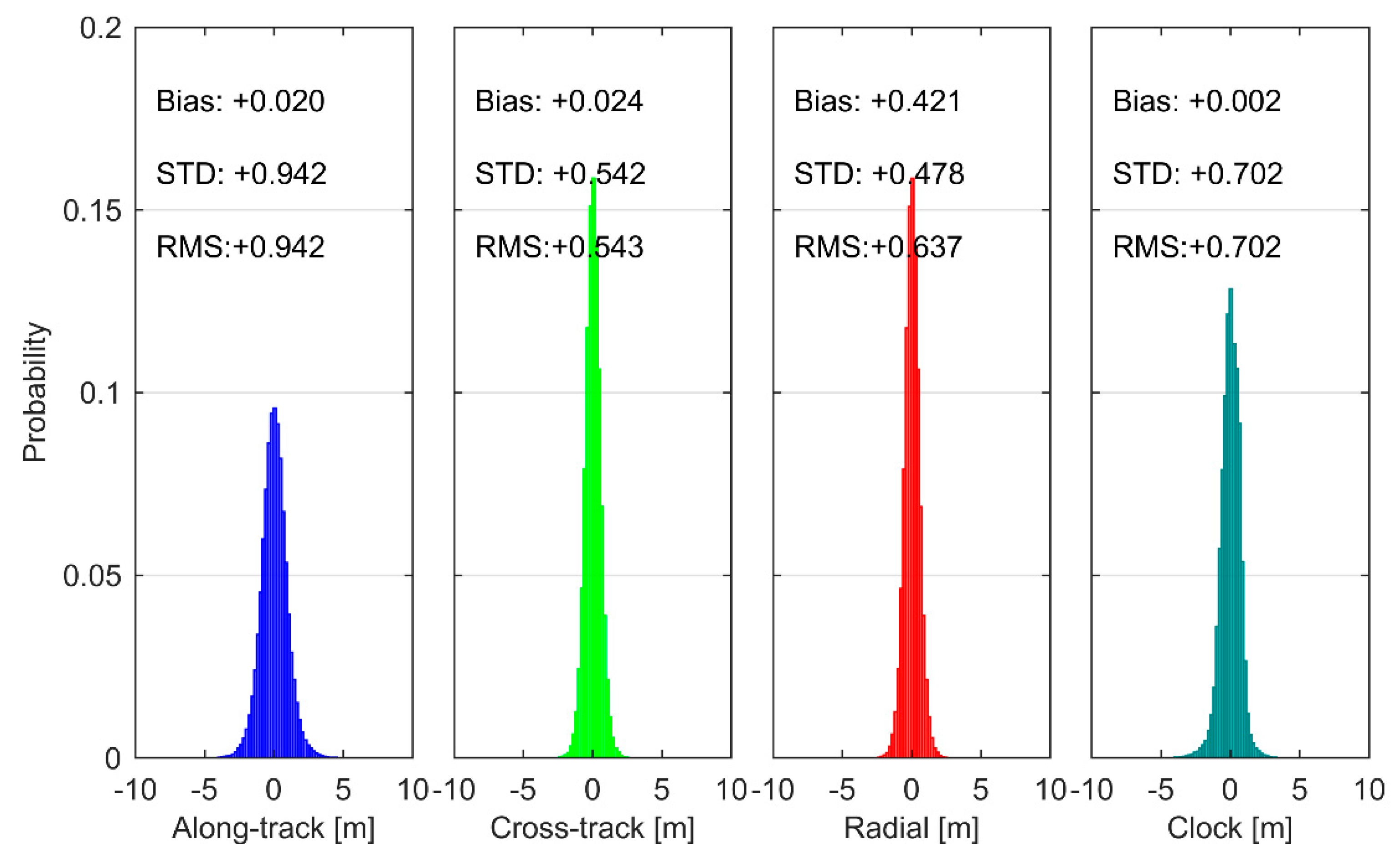
2.1.3. Signal-in-Space Range Error (SISRE) Calculation
2.2. Ionospheric Correction Evaluation Method
2.2.1. SBAS Ionospheric Correction Calculation
2.2.2. Ionospheric Correction Error Calculation
3. Experiment and Results
3.1. Evaluation Results of SBAS Orbit and Clock Corrections
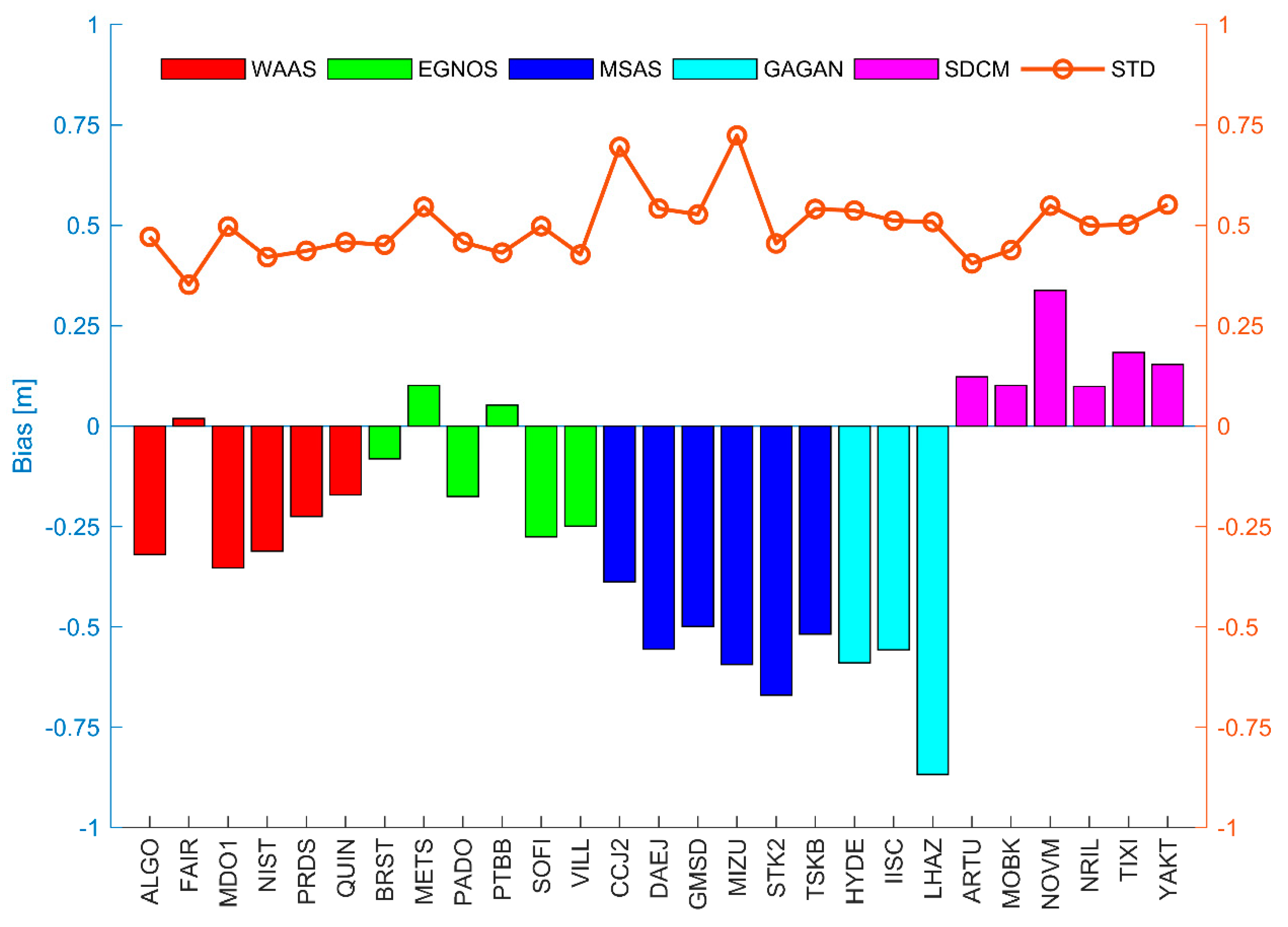
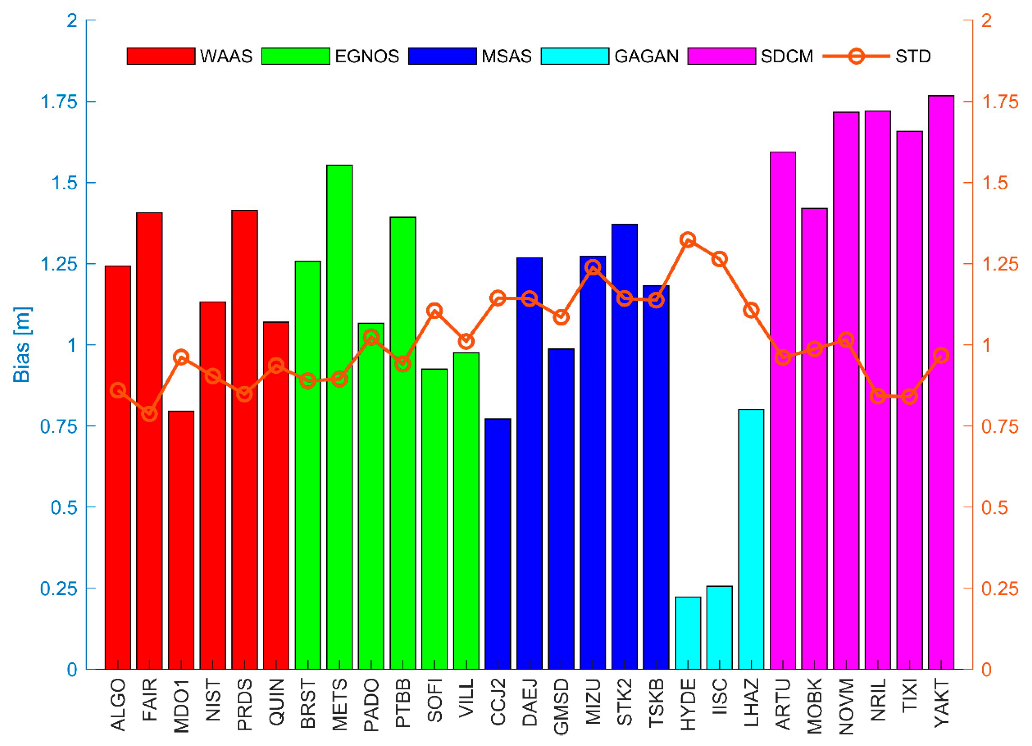
3.2. Evaluation Results of SBAS Ionospheric Corrections
4. Discussion
5. Conclusions
Author Contributions
Funding
Acknowledgments
Conflicts of Interest
References
- RTCA. Minimum Operational Performance Standards for Global Positioning System/Wide Area Augmentation System Airborne Equipment, RTCA DO-229D; Radio Technical Commission for Aeronautics (RTCA): Washington, DC, USA, 2006. [Google Scholar]
- CSNO. Development of the BeiDou Navigation Satellite System, version 3.0; China Satellite Navigation Office (CSNO): Beijing, China, 2018. [Google Scholar]
- Weber, G.; Mervart, L.; Lukes, Z.; Rocken, C.; Dousa, J. Real-time clock and orbit corrections for improved point positioning via NTRIP. In Proceedings of the ION GNSS 2007, Fort Worth, TX, USA, 25–28 September 2007; pp. 1992–1998. [Google Scholar]
- Hadas, T.; Bosy, J. IGS RTS precise orbits and clocks verification and quality degradation over time. GPS Solut. 2015, 19, 93–105. [Google Scholar] [CrossRef]
- Heßelbarth, A.; Wanninger, L. SBAS orbit and satellite clock corrections for precise point positioning. GPS Solut. 2013, 17, 465–473. [Google Scholar] [CrossRef]
- Li, L.; Jia, C.; Zhao, L.; Cheng, J.; Liu, J.; Ding, J. Real-time single frequency precise point positioning using sbas corrections. Sensors 2016, 16, 1261. [Google Scholar] [CrossRef]
- Kim, J.; Lee, Y.J. Using ionospheric corrections from the space-based augmentation systems for low earth orbiting satellites. GPS Solut. 2015, 19, 423–431. [Google Scholar] [CrossRef]
- Pungpet, P.; Kitpracha, C.; Promchot, D.; Satirapod, C. Positioning accuracy analyses on GPS single point positioning determination with GAGAN correction services in Thailand. In Proceedings of the 2018 15th International Conference on Electrical Engineering/Electronics, Computer, Telecommunications and Information Technology (ECTI-CON), Chiang Rai, Thailand, 18–21 July 2018; pp. 724–727. [Google Scholar]
- Dammalage, T.; De Silva, D.; Satirapod, C. Performance Analysis of GPS Aided Geo Augmented Navigation (GAGAN) Over Sri Lanka. Eng. J. 2017, 21, 305–314. [Google Scholar] [CrossRef]
- Marila, S.; Bhuiyan, M.Z.H.; Kuokkanen, J.; Koivula, H.; Kuusniemi, H. Performance comparison of differential GNSS, EGNOS and SDCM in different user scenarios in Finland. In Proceedings of the 2016 European Navigation Conference (ENC), Helsinki, Finland, 30 May–2 June 2016; pp. 1–7. [Google Scholar]
- Lopez, M.; Anton, V. SBAS/EGNOS enabled devices in maritime. TransNav Int. J. Mar. Navig. Saf. Sea Transp. 2018, 12, 23–27. [Google Scholar] [CrossRef]
- Laurichesse, D.; Privat, A. An open-source PPP client implementation for the CNES PPP-WIZARD demonstrator. In Proceedings of the ION GNSS+ 2015, Tampa, FL, USA, 14–18 September 2015; pp. 2780–2789. [Google Scholar]
- Rovira-Garcia, A.; Juan, J.; Sanz, J.; González-Casado, G.; Ibáñez, D. Accuracy of ionospheric models used in GNSS and SBAS: Methodology and analysis. J. Geod. 2016, 90, 229–240. [Google Scholar] [CrossRef]
- Bahrami, M.; Ffoulkes-Jones, G.; Zhang, Q. Analysis of SBAS orbit and clock corrections for GPS and their applicability to today’s mass market multi-GNSS personal navigation. In Proceedings of the ION GNSS+ 2016, Portland, OR, USA, 12–16 September 2016; pp. 2766–2776. [Google Scholar]
- Schmid, R.; Steigenberger, P.; Gendt, G.; Ge, M.; Rothacher, M. Generation of a consistent absolute phase-center correction model for GPS receiver and satellite antennas. J. Geod. 2007, 81, 781–798. [Google Scholar] [CrossRef]
- Dach, R.; Schmid, R.; Schmitz, M.; Thaller, D.; Schaer, S.; Lutz, S.; Steigenberger, P.; Wübbena, G.; Beutler, G. Improved antenna phase center models for GLONASS. GPS Solut. 2011, 15, 49–65. [Google Scholar] [CrossRef]
- Bar-Sever, Y.E. A new model for GPS yaw attitude. J. Geod. 1996, 70, 714–723. [Google Scholar] [CrossRef]
- Kouba, J. A simplified yaw-attitude model for eclipsing GPS satellites. GPS Solut. 2009, 13, 1–12. [Google Scholar] [CrossRef]
- Kuang, D.; Desai, S.; Sibois, A. Observed features of GPS Block IIF satellite yaw maneuvers and corresponding modeling. GPS Solut. 2017, 21, 739–745. [Google Scholar] [CrossRef]
- Rebischung, P.; Schmid, R. IGS14/igs14. atx: A new framework for the IGS products. In Proceedings of the AGU Fall Meeting 2016, San Francisco, CA, USA, 15 December 2016. [Google Scholar]
- FAA. Global Positioning System Wide Area Augmentation System (WAAS) Performance Standard; Federal Aviation Administration (FAA): Washington, DC, USA, 2008.
- Wong, R.F.; Rollins, C.M.; Minter, C.F. Recent updates to the WGS 84 reference frame. In Proceedings of the ION ITM GNSS 2012, Nashville, TN, USA, 17–21 September 2012; pp. 1164–1172. [Google Scholar]
- CNES; ESA; EU. User Guide for EGNOS Application Developers, ED 2.0; European Commission: Brussels, Belgium, 2011. [Google Scholar]
- RTCM Special Committee. RTCM Standard 10403.3 Differential GNSS (Global Navigation Satellite Systems) Services, version 3; RTCM Special Committee No. 104: Arlington, TX, USA, 2016. [Google Scholar]
- Takasu, T. RTKLIB ver. 2.4. 2 Manual; Tokyo University of Marine Science and Technology: Tokyo, Japan, 2013. [Google Scholar]
- Kouba, J.; Héroux, P. Precise point positioning using IGS orbit and clock products. GPS Solut. 2001, 5, 12–28. [Google Scholar] [CrossRef]
- Kouba, J. A Guide to Using International GNSS Service (IGS) Products; IGS Central Bureau: Pasadena, CA, USA, 2015. [Google Scholar]
- Montenbruck, O.; Hauschild, A. Code Biases in Multi-GNSS Point Positioning. In Proceedings of the ION ITM 2013, San Diego, CA, USA, 27–29 January 2013; pp. 616–628. [Google Scholar]
- Dach, R.; Lutz, S.; Walser, P.; Fridez, P. Bernese GNSS Software Version 5.2. User Manual; Astronomical Institute, University of Bern, Bern Open Publishing: Bern, Switzerland, 2015. [Google Scholar]
- Montenbruck, O.; Steigenberger, P.; Hauschild, A. Broadcast versus precise ephemerides: A multi-GNSS perspective. GPS Solut. 2015, 19, 321–333. [Google Scholar] [CrossRef]
- Heng, L.; Gao, G.X.; Walter, T.; Enge, P. Statistical characterization of GPS signal-in-space errors. In Proceedings of the ION ITM 2011, San Diego, CA, USA, 24–26 January 2011; pp. 312–319. [Google Scholar]
- Heng, L. Safe Satellite Navigation with Multiple Constellations: Global Monitoring of GPS and GLONASS Signal-In-Space Anomalies. Ph.D. Thesis, Stanford University, Stanford, CA, USA, 2012. [Google Scholar]
- GPS Directorate. Global Positioning System Standard Positioning Service Performance Standard, 4th ed.; Global Positioning System Directorate: Washington, DC, USA, 2008. [Google Scholar]
- Brunini, C.; Azpilicueta, F.J. Accuracy assessment of the GPS-based slant total electron content. J. Geod. 2009, 83, 773–785. [Google Scholar] [CrossRef]
- Bishop, G.; Klobuchar, J.; Doherty, P. Multipath effects on the determination of absolute ionospheric time delay from GPS signals. Radio Sci. 1985, 20, 388–396. [Google Scholar] [CrossRef]
- Mannucci, A.; Wilson, B.; Yuan, D.; Ho, C.; Lindqwister, U.; Runge, T. A global mapping technique for GPS-derived ionospheric total electron content measurements. Radio Sci. 1998, 33, 565–582. [Google Scholar] [CrossRef]
- Zhang, Q.; Zhao, Q. Global Ionosphere Mapping and Differential Code Bias Estimation during Low and High Solar Activity Periods with GIMAS Software. Remote Sens. 2018, 10, 705. [Google Scholar] [CrossRef]
- Li, Z.; Yuan, Y.; Wang, N.; Hernandez-Pajares, M.; Huo, X. SHPTS: Towards a new method for generating precise global ionospheric TEC map based on spherical harmonic and generalized trigonometric series functions. J. Geod. 2015, 89, 331–345. [Google Scholar] [CrossRef]
- Schaer, S. Mapping and Predicting the Earth’s Ionosphere Using the Global Positioning System. Ph.D. Thesis, University of Bern, Bern, Switzerland, 1999. [Google Scholar]
- Lanyi, G.E.; Roth, T. A comparison of mapped and measured total ionospheric electron content using global positioning system and beacon satellite observations. Radio Sci. 1988, 23, 483–492. [Google Scholar] [CrossRef]
- Suard, N.; Gurtner, W.; Estey, L. Proposal for a new RINEX-type Exchange File for GEO SBAS Broadcast Data; UNAVCO: Boulder, CO, USA, 2004. [Google Scholar]
- Yousif, H.; El-Rabbany, A. Assessment of several interpolation methods for precise GPS orbit. J. Navig. 2007, 60, 443–455. [Google Scholar] [CrossRef]
- Teunissen, P.; Montenbruck, O. Springer Handbook of Global Navigation Satellite Systems; Springer International Publishing AG: Cham, Switzerland, 2017. [Google Scholar]
- Klobuchar, J.A. Ionospheric Time-Delay Algorithm for Single-Frequency GPS Users. IEEE Trans. Aerosp. Electron. Syst. 1987, 23, 325–331. [Google Scholar] [CrossRef]
- Thomsen, M. Why Kp is such a good measure of magnetospheric convection. Space Weather 2004, 2. [Google Scholar] [CrossRef]
- Gonzalez, W.; Joselyn, J.A.; Kamide, Y.; Kroehl, H.W.; Rostoker, G.; Tsurutani, B.; Vasyliunas, V. What is a geomagnetic storm? J. Geophys. Res. Space Phys. 1994, 99, 5771–5792. [Google Scholar] [CrossRef]
- Nie, Z.; Yang, H.; Zhou, P.; Gao, Y.; Wang, Z. Quality assessment of CNES real-time ionospheric products. GPS Solut. 2019, 23, 11. [Google Scholar] [CrossRef]


| System | WAAS | EGNOS | MSAS | GAGAN | SDCM | |||||
|---|---|---|---|---|---|---|---|---|---|---|
| PRN | 135 | 138 | 120 | 123 | 129 | 137 | 127 | 128 | 125 | 140 |
| Number of missing epochs | 3 | 0 | 187 | 171 | 11,284 | 1361 | 9853 | 626,877 | 2,212,623 | 880,653 |
| Type | WAAS | EGNOS | MSAS | GAGAN | SDCM | GPS Broadcast | |||||
|---|---|---|---|---|---|---|---|---|---|---|---|
| PRN | 135 | 138 | 120 | 123 | 129 | 137 | 127 | 128 | 125 | 140 | |
| SISRE | 0.954 | 0.954 | 0.646 | 0.645 | 1.931 | 1.931 | 1.336 | 1.313 | 0.634 | 0.666 | 0.695 |
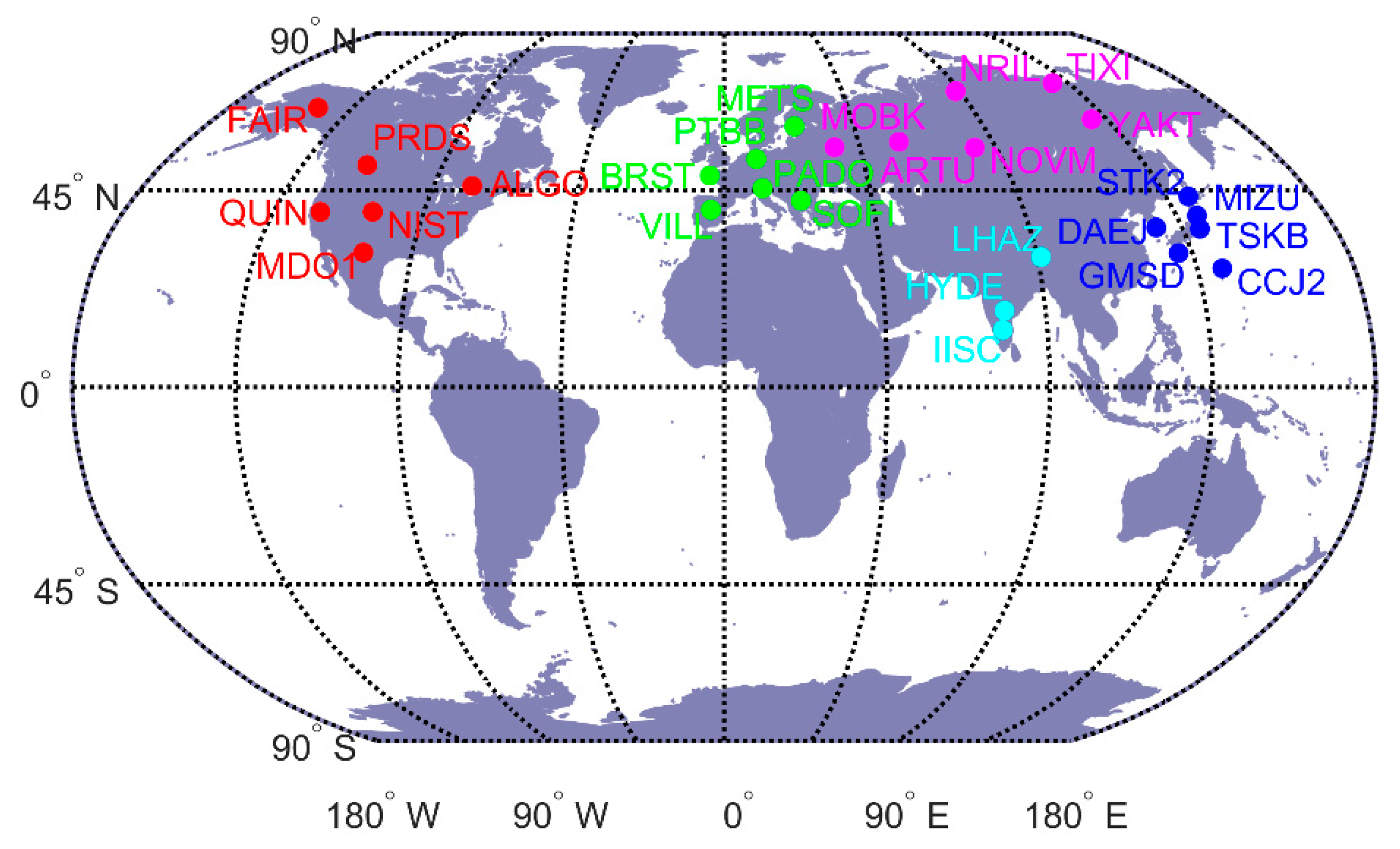
| WAAS | Station | ALGO | FAIR | MDO1 | NIST | PRDS | QUIN |
| Code signals | P1+P2 | P1+P2 | P1+P2 | C1+P2 | P1+P2 | P1+P2 | |
| EGNOS | Station | BRST | METS | PADO | PTBB | SOFI | VILL |
| Code signals | C1/P1+P2 1 | P1+P2 | P1+P2 | P1+P2 | C1+P2 | P1+P2 | |
| MSAS | Station | CCJ2 | DAEJ | GMSD | MIZU | STK2 | TSKB |
| Code signals | C1+P2 | C1+P2 | C1+P2 | P1+P2 | C1+P2 | C1+P2 | |
| GAGAN | Station | HYDE | IISC | LHAZ | |||
| Code signals | C1+P2 | P1+P2 | C1+P2 | ||||
| SDCM | Station | ARTU | MOBK | NOVM | NRIL | TIXI | YAKT |
| Code signals | P1+P2 | P1+P2 | P1+P2 | P1+P2 | P1+P2 | P1+P2 |
© 2019 by the authors. Licensee MDPI, Basel, Switzerland. This article is an open access article distributed under the terms and conditions of the Creative Commons Attribution (CC BY) license (http://creativecommons.org/licenses/by/4.0/).
Share and Cite
Nie, Z.; Zhou, P.; Liu, F.; Wang, Z.; Gao, Y. Evaluation of Orbit, Clock and Ionospheric Corrections from Five Currently Available SBAS L1 Services: Methodology and Analysis. Remote Sens. 2019, 11, 411. https://doi.org/10.3390/rs11040411
Nie Z, Zhou P, Liu F, Wang Z, Gao Y. Evaluation of Orbit, Clock and Ionospheric Corrections from Five Currently Available SBAS L1 Services: Methodology and Analysis. Remote Sensing. 2019; 11(4):411. https://doi.org/10.3390/rs11040411
Chicago/Turabian StyleNie, Zhixi, Peiyuan Zhou, Fei Liu, Zhenjie Wang, and Yang Gao. 2019. "Evaluation of Orbit, Clock and Ionospheric Corrections from Five Currently Available SBAS L1 Services: Methodology and Analysis" Remote Sensing 11, no. 4: 411. https://doi.org/10.3390/rs11040411
APA StyleNie, Z., Zhou, P., Liu, F., Wang, Z., & Gao, Y. (2019). Evaluation of Orbit, Clock and Ionospheric Corrections from Five Currently Available SBAS L1 Services: Methodology and Analysis. Remote Sensing, 11(4), 411. https://doi.org/10.3390/rs11040411