Unsupervised Sub-Pixel Water Body Mapping with Sentinel-3 OLCI Image

Abstract

Mapping land surface water bodies from satellite images is superior to conventional in situ measurements. With the mission of long-term and high-frequency water quality monitoring, the launch of the Ocean and Land Colour Instrument (OLCI) onboard Sentinel-3A and Sentinel-3B provides the best possible approach for near real-time land surface water body mapping. Sentinel-3 OLCI contains 21 bands ranging from visible to near-infrared, but the spatial resolution is limited to 300 m, which may include lots of mixed pixels around the boundaries. Sub-pixel mapping (SPM) provides a good solution for the mixed pixel problem in water body mapping. In this paper, an unsupervised sub-pixel water body mapping (USWBM) method was proposed particularly for the Sentinel-3 OLCI image, and it aims to produce a finer spatial resolution (e.g., 30 m) water body map from the multispectral image. Instead of using the fraction maps of water/non-water or multispectral images combined with endmembers of water/non-water classes as input, USWBM directly uses the spectral water index images of the Normalized Difference Water Index (NDWI) extracted from the Sentinel-3 OLCI image as input and produces a water body map at the target finer spatial resolution. Without the collection of endmembers, USWBM accomplished the unsupervised process by developing a multi-scale spatial dependence based on an unsupervised sub-pixel Fuzzy C-means (FCM) clustering algorithm. In both validations in the Tibet Plate lake and Poyang lake, USWBM produced more accurate water body maps than the other pixel and sub-pixel based water body mapping methods. The proposed USWBM, therefore, has great potential to support near real-time sub-pixel water body mapping with the Sentinel-3 OLCI image.

1. Introduction

For the observations of natural water on Earth’s surface, satellite sensors, including the Sea-viewing Wide Field-of-view Sensor (SeaWiFS), the Medium Resolution Imaging Spectrometer (MERIS) and Moderate resolution Imaging Spectroradiometer (MODIS), have been applied widely to provide near real-time dynamics of water surfaces [1,2], due to their very fine temporal resolution (e.g., 1–3 days). Unfortunately, SeaWiFS and MERIS stopped working in 2010 and 2012, respectively, and MODIS has been in service for an extended period of time. As a follow up to the SeaWiFS, MERIS, and MODIS, the recently launched Ocean and Land Colour Instrument (OLCI) onboard the European Space Agency (ESA) Sentinel-3A and Sentinel-3B satellites is the next generation imaging spectrometer for coastal and inland waters remote sensing, and it will supply operational monitoring of the Earth’s water surfaces [2,3].

As a heritage from MERIS, Sentinel-3 OLCI has identified the key deficiencies of MERIS and has undergone many improvements [4,5,6]. For the OLCI instrument, the double satellite system will enable a short revisit time of less than two days, and there are 21 spectral bands with wavelengths ranging from the optical to near-infrared in OLCI. Moreover, many spectral bands were designed for some specific functions, as listed in

Table 1. Band characteristics of the Sentinel-3 OLCI. (Source: Sentinel-3 User Handbook).

Band	Wavelength Range (nm)	Function
Oa1	392.5–407.5	Aerosol correction, improved water constituent retrieval
Oa2	407.5–417.5	Yellow substance and detrital pigments (turbidity)
Oa3	437.5–447.5	Chlorophyll (Chl )absorption max., biogeochemistry, vegetation
Oa4	485–495	High Chl, other pigments
Oa5	505–515	Chl, sediment, turbidity, red tide
Oa6	555–565	Chl reference (Chl minimum)
Oa7	615–625	Sediment loading
Oa8	660–670	Chl (2nd Chl abs. max.), sediment, yellow substance/vegetation
Oa9	670–677.5	For improved fluorescence retrieval and to better account for smile together with the bands 665 and 680 nm
Oa10	677.5–682	Chl fluorescence peak, red edge
Oa11	703.75–713.75	Chl fluorescence baseline, red edge transition
Oa12	750–757.5	O2 absorption/clouds, vegetation
Oa13	760–762.5	O2 absorption band/aerosol correction
Oa14	762.5–766.25	Atmospheric correction
Oa15	766.25–768.75	O2A used for cloud top pressure, fluorescence over land
Oa16	771.25–786.25	Atmos. corr./aerosol correction
Oa17	855–876	Atmos. corr./aerosol corr., clouds, pixel co-registration
Oa18	880–890	Water vapour absorption reference band. Common reference band with SLSTR instrument. Vegetation monitoring
Oa19	895–905	Water vapour absorption/vegetation monitoring (max. reflectance)
Oa20	930–950	Water vapour absorption, atmos./aerosol corr.
Oa21	1000–1040	Atmos./aerosol correction

. Given such great characteristics, Sentinel-3 OLCI image haas been applied to retrieval biophysical parameters [7], estimate crop and grass chlorophyll and nitrogen content [8], map water quality parameters [3], classify natural colours of water [2], estimate green leaf area index in C3 and C4 crops [9], determine the downwelling diffuse attenuation coefficient of lake water [10], and map colored dissolved organic matters [11]. With respect to the above applications, most of them were done using the Sentinel-3 OLCI image for quantitative inversion, as it can generate more continuous spectral curves than many other satellite sensors, such as MODIS, Landsat Thematic Mapper (TM), Enhanced Thematic Mapper Plus (ETM+), Operational Land Imager (OLI). However, it is of great interest for Sentinel-3 OLCI to map water bodies because it has many spectral bands that are sensitive to the water surface and are able to provide near real-time water body monitoring.

In terms of remote sensing applications, water body mapping from coarse spatial resolution but fine temporal resolution satellite images including MERIS and MODIS has attracted much attention [12,13,14,15,16,17,18,19]. However, to the best of our knowledge, there are few papers focusing on water body mapping with the Sentinel-3 OLCI image so far. Generally, various methods can be applied to map water bodies from Sentinel-3 OLCI image, such as single band density segmentation [20], water body classification [21,22], spectral unmixing [16,23] and spectral water indexes (such as the Normalized Difference Water Index, NDWI) [24,25,26,27,28]. However, these methods can only extract water body extent at the per-pixel scale, but the spatial resolution of Sentinel-3 is only 300 m, which is insufficient to exploit detailed water body features in real applications.

Sub-pixel mapping (SPM), also termed super-resolution mapping (SRM), is a method employed to produce a finer spatial resolution land cover map than the input fractional land cover maps or multispectral images [29,30,31]. From this point of view, SPM can, therefore, be used to produce finer spatial resolution water body maps from Sentinel-3 OLCI image. During the past decades, SPM has been applied successfully to produce water body maps at the sub-pixel scale. For example, Ling [32] developed an SPM method that can use digital elevation models (DEM) as auxiliary data to generate sub-pixel water body map, Muad and Foody [33] proposed an SPM method to extract water surface of lakes from coarse spatial and fine temporal resolution satellite images, Huang et al. [34] improved the traditional pixel-swapping based SPM method to enhance floodplain inundation mapping, Li et al. [35] proposed a sub-pixel flood inundation mapping method based on discrete particle swarm optimization, Li et al. [36] proposed an SPM method to map wetland inundation at sub-pixel scale based on back-propagation neural network and genetic algorithm, and Li et al. [37] proposed a locally adaptive SPM method to extract waterline from MODIS images. Fortunately, almost all of these SPM models developed for sub-pixel water body mapping are supervised methods, and additional operations, such as endmember extraction of various land cover classes and spectral unmixing, are required. For the supervised SPM methods, the selection of training samples or endmembers is often subjective and time-consuming, and it has become urgent to extract sub-pixel water body map with an unsupervised method [38,39].

In this paper, an unsupervised sub-pixel water body mapping (USWBM) method was proposed for Sentinel-3 OLCI image. Different from the traditional supervised SPM methods, USWBM is an unsupervised SPM method, and there is no need for it to collect a training dataset or endmembers for water and non-water classes. Implementation of USWBM was based on three main terms: spectral water index term, sub-pixel water spatial dependence term, and coarse-pixel water spatial dependence term. Specifically, the spectral water index term is based on the Fuzzy C-means (FCM) clustering [40], the sub-pixel water spatial dependence term is based on the maximal spatial-dependence model [30], and the coarse-pixel water spatial dependence term is based on the radial basis function (RBF) downscaling [41,42,43]. Instead of using the multispectral image of Sentinel-3 OLCI or the water fractional map extracted from Sentinel-3 OLCI image as input, USWBM can use directly the spectral water indexes calculated from Sentinel-3 OLCI image as input, and the output is a finer spatial resolution (e.g., 30 m) water body map.

The main objectives of this research are: (1) validate the performance of multi-scale (pixel and sub-pixel scales) water body mapping with the newly launched Sentinel-3 OLCI image, so as to promote the application of the Sentinel-3 OLCI image in water body mapping; (2) explore unsupervised SPM methods that could use directly the spectral water indexes (NDWI images) as input to produce sub-pixel water body maps, where traditional water body mapping with SPM methods was using multispectral images or fractional land cover maps as input; (3) propose an unsupervised sub-pixel water body mapping method (USWBM) based on both the sub-pixel and coarse-pixel spatial dependence to produce a water body map from four integrated NDWI images of Sentinel-3 OLCI image. The remainder of this paper is organized as follows: Section 2 introduces the proposed USWBM method, Section 3 reports the experimental results and discussion, and Section 4 draws the conclusions.

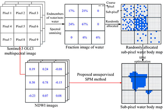
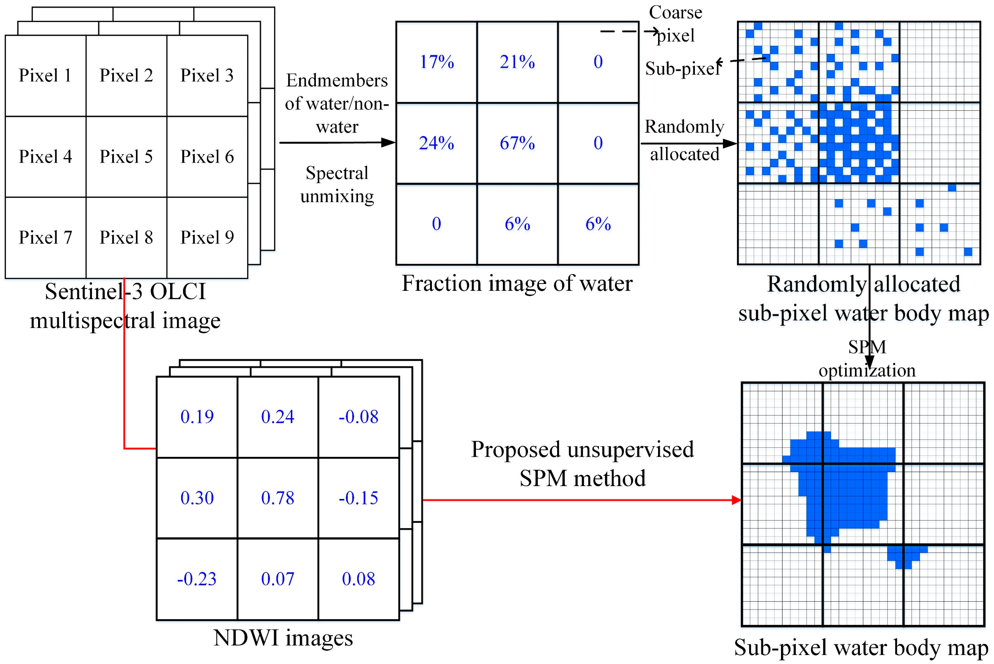
2. Sub-Pixel Water Body Mapping with SPM

Given a Sentinel-3 OLCI multispectral image, traditional supervised SPM methods can be used to produce a water body map from it. As shown in Figure 1, assume that the fraction image of water has been obtained by using a spectral unmixing algorithm, such as the linear spectral mixture model [44]. The spatial scale between the Sentinel-3 OLCI image and the resultant fine spatial resolution sub-pixel water body map is defined as 10, and then each coarse pixel in the water fraction image is divided into 10 × 10 sub-pixels. First, the water fraction image is transformed into the randomly allocated sub-pixel water body map, where each of the sub-pixels is allocated randomly within each coarse pixel, and the number of sub-pixels within each coarse pixel is calculated from the water fraction image. If the fraction value of a coarse pixel in water fraction image is 67%, and then there will be 10 × 10 × 67% = 67 sub-pixels in the coarse pixel. However, the randomly allocated sub-pixel water body map does not follow the real-world spatial distribution of water features. The sub-pixel maximal spatial dependence principle [45] is used widely to allocate the spatial distribution of water class, and this is indeed the process of SPM optimization, which can be completed by using many SPM methods, such as the pixel-swapping (PS) [30] and the Hopfield neural network (HNN) [46].

As mentioned above, endmember collection of water and non-water classes in traditional supervised SPM methods is often subjective and time-consuming, and the sub-pixel water body map needs to be extracted with an unsupervised method. Motivated by the pixel-scale water body mapping methods based on a spectral water index (such as NDWI), this research aims to produce a sub-pixel water body map directly from the coarse spatial resolution NDWI images extracted from Sentinel-3 OLCI image. Particularly, as represented in Figure 1, an unsupervised SPM method was proposed, and more detail about it is reported in the following section.

3. Methods

Figure 2 represents the flowchart of the proposed USWBM approach. Once the data pre-processing has been conducted for the Sentinel-3 OLCI image, the green band 6 and near-infrared (NIR) bands 17-20 can then be used to calculate the NDWI images, which are regarded as the input data of the USWBM model. In general, band 17 in Sentinel-3 OLCI is always seen as the NIR band to calculate the NDWI image. However, compared with Landsat TM, ETM+ and OLI, the wavelength range of band 17 of Sentinel-3 OLCI is too narrow, and the NIR bands in Landsat TM, ETM+ and OLI images basically cover bands 17, 18, 19 and 20 of Sentinel-3 OLCI. In order to have a comprehensive response to the water features, all of the NDWI images calculated from green band 6 and NIR bands 17–20 are used as the input for USWBM. The implementation of USWBM is composed of the following three terms.

3.1. The Objective Function of USWBM

Let $Y=\left[y_1,y_2,\cdots ,y_N\right]$ be the input vector that is composed of the N NDWI images of $y_1$, $y_2$, …, $y_N$. The NDWI images were extracted from Sentinel-3 OLCI image with spatial resolution R. Assuming the spatial scale as $z$, the proposed USWBM aims to produce water body map X with a spatial resolution of $R/z$, where each coarse pixel in $Y$ contains $z\times z$ fine pixels in X. The objective function of USWBM is completed as a minimize optimization problem that is composed of three terms, and it is expressed as:

$$\widehat{X}=\arg \left\{\underset{X}{\min }(U_{index}+\lambda U_{SD}+\delta U_{CD})\right\}$$

(1)

where $U_{index}$ is the function of spectral water index term, $U_{SD}$ is the function of sub-pixel water spatial dependence term, and $U_{CD}$ is the function of coarse-pixel water spatial dependence term. $\lambda$ and $\delta$ are two trade-off parameters used to balance the contributions of the three terms.

3.2. The Spectral Water Index Term

The spectral water index term in USWBM is used to match the class proportions of water and non-water in the output fine spatial resolution water body map X to the input NDWI images $Y$, and make a strong relationship between them. Given that FCM can provide fuzzy membership values correlated with the class area proportions [40,47], the spectral water index term was, therefore, developed based on the unsupervised FCM clustering. The objective function of the spectral water index term $U_{index}$ is formulated to minimize the energy function:

$$U_{index}={\displaystyle \sum _{j=1}^M{\displaystyle \sum _{c=1}^C(f_c(x_j)}}{)}^m\times {\Vert y_{x_j}-v_c\Vert }^2,$$

(2)

where $M$ is the number of coarse pixels in the NDWI image, $x_j$ is one coarse pixel in the NDWI image, $C$ is the number of land cover classes in the fine spatial resolution water body map X ($C$ = 2, as there are only water and non-water classes in X), $f_c(x_j)$ is the fraction value of class c in the coarse pixel $x_j$ and is calculated by Equation (3):

$$\begin{array}{cc}{f}_c(x_j)={\displaystyle \sum _{i=1}^{z^2}{\displaystyle \sum _{c=1}^C{\eta }_c(x_i,x_j)}}/z^2,& j=1,2,\cdots ,M,\end{array}$$

(3)

$m$ is a weighting exponent parameter used to control the clustering fuzziness. It is noted that when $m$ approaches 1, the value of $f_c(x_j)$ would be equal to 1; and when $m$ approaches $\infty$, the value of $f_c(x_j)$ would be equal to $1/C$. ${\eta }_c(x_i,x_j)$ is the labeled value of sub-pixel $x_i$ in each coarse pixel $x_j$ and is calculated by Equation (4):

$${\eta }_c(x_i,x_j)=\{\begin{array}{cc}1\hfill & \mathrm{if} \mathrm{sub-pixel} x_i \mathrm{in} \mathrm{coarse} \mathrm{pixel} x_j \mathrm{is} \mathrm{assigned} \mathrm{to} \mathrm{class} c\\ 0\hfill & \mathrm{otherwise}\end{array},$$

(4)

$v_c$ is a vector containing the clustering centers for different land cover classes and is calculated by Equation (5):

$$\begin{array}{cc}{v}_c=\frac{{\displaystyle {\sum }_{j=1}^M{(f_c(x_j))}^m·y_{x_j}}}{{\displaystyle {\sum }_{j=1}^M{(f_c(x_j))}^m}},& c=1,2,\cdots ,C.\end{array}$$

(5)

3.3. The Sub-Pixel Water Spatial Dependence Term

The sub-pixel water spatial dependence term is used to make the resultant fine spatial resolution water body map locally smooth. In SPM, it is always assumed that there is a tendency for spatially proximate observations of a given property to be more similar than those of more distant observations [29,30]. This assumption is also suitable for the class of water, as the spatial distribution of the water class is often spatial aggregation. The class label of the target fine pixel is, therefore, determined by the classes of the neighboring sub-pixels [32,34]. Based on this assumption, the objective function of sub-pixel water spatial dependence term is formulated as the following function:

$$U_{SD}=-{\displaystyle \sum _{j=1}^M{\displaystyle \sum _{c=1}^C{\displaystyle \sum _{i=1}^{z^2}{\eta }_c(x_i,x_j)\times D_c(x_i,x_j)}}},$$

(6)

where ${\eta }_c(x_i,x_j)$ is the labeled value of sub-pixel $x_i$ in the coarse pixel $x_j$, and each sub-pixel can only belong to one certain class. $D_c(x_i,x_j)$ is the spatial dependence values for the fine pixel $x_i$ in coarse pixel $x_j$ when the fine pixel $x_i$ is assigned as land cover class c, and it is calculated as the distance-weighted function that is expressed as:

$$D_c(x_i,x_j)={\displaystyle \sum _{t=1}^{N_{\mathrm{sp}}}\gamma (x_i,x_t){\eta }_c(x_t)},$$

(7)

$$\gamma (x_i,x_t)=\exp (-d(x_i,x_t)/\theta ),$$

(8)

$${\eta }_c(x_t)=\{\begin{array}{cc}1\hfill & \mathrm{if} \mathrm{sub-pixel} x_t \mathrm{is} \mathrm{assigned} \mathrm{to} \mathrm{class} c\\ 0& \mathrm{otherwise}\end{array},$$

(9)

where $N_{sp}$ is the number of sub-pixels in the sub-pixel neighboring system for the target fine pixel $x_i$ and is composed of $w\times w$ fine pixels. ${\eta }_c(x_t)$ is the class label for sub-pixel $x_t$ in the neighboring system and is calculated by Equation (9). $\gamma (x_i,x_t)$ is the distance weight between target fine pixel $x_i$ and its neighboring fine pixels $x_t$, and it is calculated by Equation (8). $d(x_i,x_t)$ is the geometric distance between the target fine pixel $x_i$ and its neighboring fine pixels $x_t$, and $\theta$ is the nonlinear parameter of the distance decay model.

3.4. The Coarse-Pixel Water Spatial Dependence Term

Compared with the sub-pixel water spatial dependence term, the coarse-pixel water spatial dependence term aims to provide holistic information about water class for the resultant water body map. The class label of the target fine pixel is, therefore, determined by the class labels of its neighboring coarse-pixels. The objective function of the coarse-pixel water spatial dependence term is, therefore, to achieve the maximal value of the spatial corrections of neighboring coarse-pixels. Specially, the RBF downscaling [42] was adapted here to construct the coarse-pixel water spatial dependence term, and it is expressed as:

$$U_{CD}=-{\displaystyle \sum _{j=1}^M{\displaystyle \sum _{c=1}^C{\displaystyle \sum _{i=1}^{z^2}{\displaystyle \sum _{l=1}^{N_{cp}}{\alpha }_c(x_i,x_l)\varphi (x_i,x_l)}}}},$$

(10)

where $N_{cp}$ is the number of coarse pixels in the coarse-pixel neighboring system of fine pixel $x_i$, and it is composed of W × W coarse pixels centered at fine pixel $x_i$. ${\alpha }_c(x_i,x_l)$ is the spatial coefficient of between fine pixel $x_i$ and coarse pixel $x_l$ at the class label of c. $\varphi (x_i,x_l)$ is used to measure the geolocation relationship between the coarse pixel $x_l$ and the target fine pixel $x_i$, and it is always formulated as the Gaussian function and expressed as:

$$\varphi (x_i,x_l)=\exp [-d^2(x_i,x_l)/{\varpi }^2],$$

(11)

where $\varpi$ is the distance-decay parameter used to control the contribution of neighboring pixels, $d(x_i,x_l)$ is the geometric distance between the fine pixel $x_i$ and its neighboring coarse pixels $x_l$.

The calculation of spatial coefficient ${\alpha }_c(x_i,x_l)$ is achieved through the solution of prior information contained in the other coarse-pixels in the neighboring system. Let $x_p$ be another coarse pixel in the same coarse-pixel neighboring system of fine pixel $x_i$, and ${\alpha }_c(x_i,x_l)$ is then expressed as:

$$\begin{array}{cc}{f}_c(x_l)={\displaystyle \sum _{p=1}^{N_{cp}}{\alpha }_c(x_i,x_l)\varphi (x_p,x_l)},& l=1,2,\cdots ,N_{cp},\end{array}$$

(12)

where $\varphi (x_p,x_l)$ is the geolocation relationship between the coarse pixel $x_l$ and the coarse pixel $x_p$, and it can be calculated by Equation (11). As $f_c(x_l)$ and $\varphi (x_p,x_l)$ are already known, the solution of ${\alpha }_c(x_i,x_l)$ could be solved by the following matrix Equation (13):

$$\left[\begin{array}{ccc}\varphi (x_1,x_1)& \cdots & \varphi (x_1,x_{N_{cp}})\\ \varphi (x_2,x_1)& \cdots & \varphi (x_2,x_{N_{cp}})\\ & ⋮& \\ \varphi (x_{N_{cp}},x_1)& \cdots & \varphi (x_{N_{cp}},x_{N_{cp}})\end{array}\right]\left[\begin{array}{c}{\alpha }_c(x_i,x_1)\\ {\alpha }_c(x_i,x_2)\\ ⋮\\ {\alpha }_c(x_i,x_{N_{cp}})\end{array}\right]=\left[\begin{array}{c}{f}_c(x_1)\\ f_c(x_2)\\ ⋮\\ f_c(x_{N_{cp}})\end{array}\right].$$

(13)

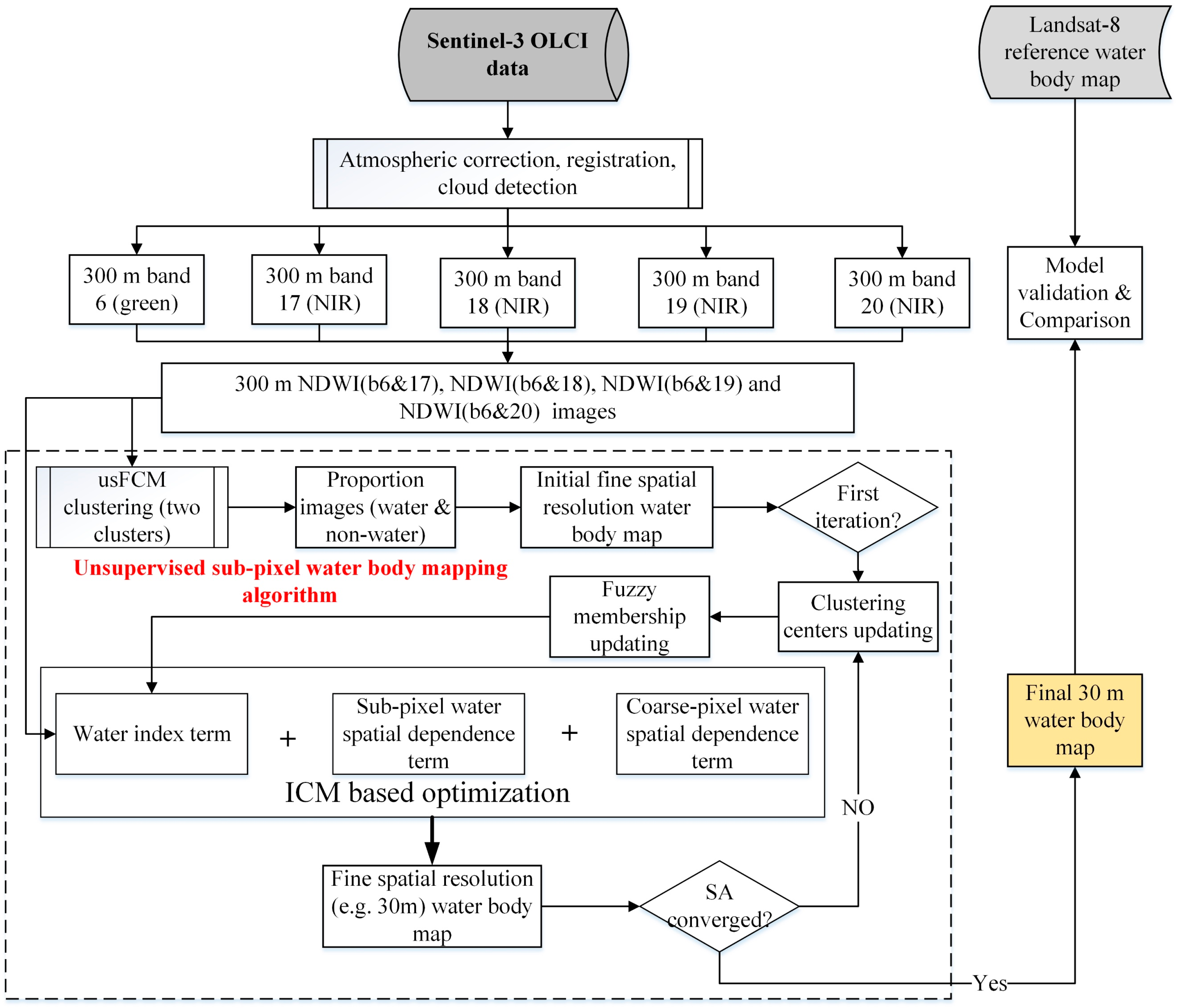
3.5. Implementation of USWBM

The goal of the objective function of USWBM shown in Equation (1) is to obtain the minimize value, and the widely used simulated annealing algorithm (SA) [1] is applied to find the solution of this minimize optimization problem. Generally, the annealing schedule is expressed as a power-law decay function:

$$T_n=\sigma ·T_{n-1},$$

(14)

where $T_n$ and $T_{n-1}$ are the temperature values of two adjacent iterations, $\sigma \in (0,1)$ controls the rate of temperature decrease during the iterations. Based on this, the proposed USWBM algorithm is implemented through the following steps:

(1)

Pre-process the Sentinel-3 OLCI data, and extract the four NDWI images based on the band 6 and bands 17–20. Set the scale factor $z$, the values of key parameters $m$, $\lambda$ and $\delta$, the maximum iteration number $t_{\max }$, and the starting temperature $T_0$.

(2)

Randomly label the sub-pixels within each coarse pixel as water or non-water classes, so as to generate an initialized sub-pixel water body map.

(3)

Obtain the fraction value $f_c(x_j)$ and the clustering center vector $v_c$ for the initialized sub-pixel water body map via Equations (3) and (5), and then calculate the objective function value shown in Equation (1).

(4)

Decrease the temperature $T$, the class labels of all the sub-pixels in the sub-pixel water body map are changed in terms of a row-wise visiting scheme, and update the fraction value $f_c(x_j)$ and the clustering center vector $v_c$.

(5)

End the iteration by reaching $t_{\max }$, or when no less than 0.1% of the sub-pixel labels are changed between two iterations; otherwise, steps 4 is repeated.

4. Experiment Results and Discussion

4.1. Experiment Setup

4.1.1. Datasets Pre-Processing

In order to have a comprehensive validation of the performance of USWBM, two typical study sites located at the northern Tibet Plate and Poyang lake were chosen. The total area of Tibet Plate lakes is 36,899 km², accounting for 45.2% of the total lake area in China; it is the highest and largest inland lake area on the earth and is also one of the two lake areas with the highest density in China. The Poyang lake is China’s largest freshwater lake, located in the northern part of Jiangxi Province, with an area of 4125 km²; the water level and lake area of Poyang lake vary greatly during the year, but play a huge role in regulating the water level of the Yangtze River, conserving water sources, improving the local climate and maintaining the ecological balance of the surrounding areas.

As shown in Figure 3, two subset Sentinel-3 OLCI images covering the Tibet Plate lake and Poyang lake were used in the experiments. Specifically, two Sentinel-3 OLCI images were acquired on 2 and 11 August 2017 and downloaded from the ESA (https://scihub.copernicus.eu/). With the Sentinel Toolboxes of Sentinel Application Platform (SNAP), the particular data pre-processing of atmospheric correction, coordinate transformation, and cloud detection was done for the two used Sentinel-3 OLCI images. Each of the subset Sentinel-3 OLCI images contains 40 × 40 pixels covering an area of 12 km × 12 km. For the validation, the Landsat-8 OLI images acquired on August 2 and 11, 2017 (it is the same acquisition time as the two Sentinel-3 OLCI images, so as to ensure the water level in Sentinel-3 OLCI and MODIS images is the same) were used to extract reference water body maps for the two study sites. Two Landsat-8 OLI images were downloaded as the surface reflectance product from USGS Earth Explorer (https://earthexplorer.usgs.gov/). Each subset of the Landsat-8 images and reference water body maps contains 400 × 400 pixels, and they are shown in Figure 3. The NIR band (band 5) and Green band (band 3) of Landsat-8 OLI images were used to generate the NDWI images, and then OTSU segmentation was used to produce the reference water body maps.

It is noted that as Landsat-8 images were used as the reference, the Sentinel-3 OLCI images were reprojected into the same Geographic Reference System of the original Landsat-8 images, that is WGS84 UTM Zone 45N and WGS84 UTM Zone 50N for the Tibet Plate lake and Poyang lake, respectively. Moreover, geometric registration between Landsat-8 and Sentinel-3 OLCI images was completed with the “Georeferencing” tool in ARCGIS. For each of the study sites, 5 to 8 control points were selected from the stable but distinct surface features, such as bare rock, a large dam and a bridge.

4.1.2. Accuracy Assessment

In this research, 30 m water body maps extracted from Landsat-8 OLI images were used as the reference, and all of the pixels (400 × 400 pixels) in the reference water body maps (see Figure 3) were used for accuracy assessment. The proposed USWBM algorithm aims to produce 30 m water body maps from the multi-frame NDWI images of Sentinel-3 OLCI image. Map-level accuracy indices of the Kappa coefficient, overall accuracy (OA) and the class-level accuracy indices of omission and commission error for water class were used for quantitative assessment. Moreover, coherence between the results of different algorithms and the reference water body maps was also used for quantitative assessment. Both of the pixel and sub-pixel-based water body mapping methods were used as the comparison against the proposed USWBM algorithm. Specifically, the segmentation algorithm based on the OTSU algorithm [24,48] and the unsupervised FCM clustering [49] were used to extract a 300 m water body map from the NDWI images of Sentinel-3 OLCI image. The unsupervised sub-pixel mapping method based on FCM clustering (usFCM_SPM) [40] was used to produce a 30 m water body map from the NDWI images. Similar to the proposed algorithm, usFCM_SPM is composed of the FCM clustering based spectral term and sub-pixel maximal spatial dependence based spatial term. The 30 m water body map could be generated from the input NDWI images by optimizing the integrated spectral and spatial terms, and more details can be found in [40].

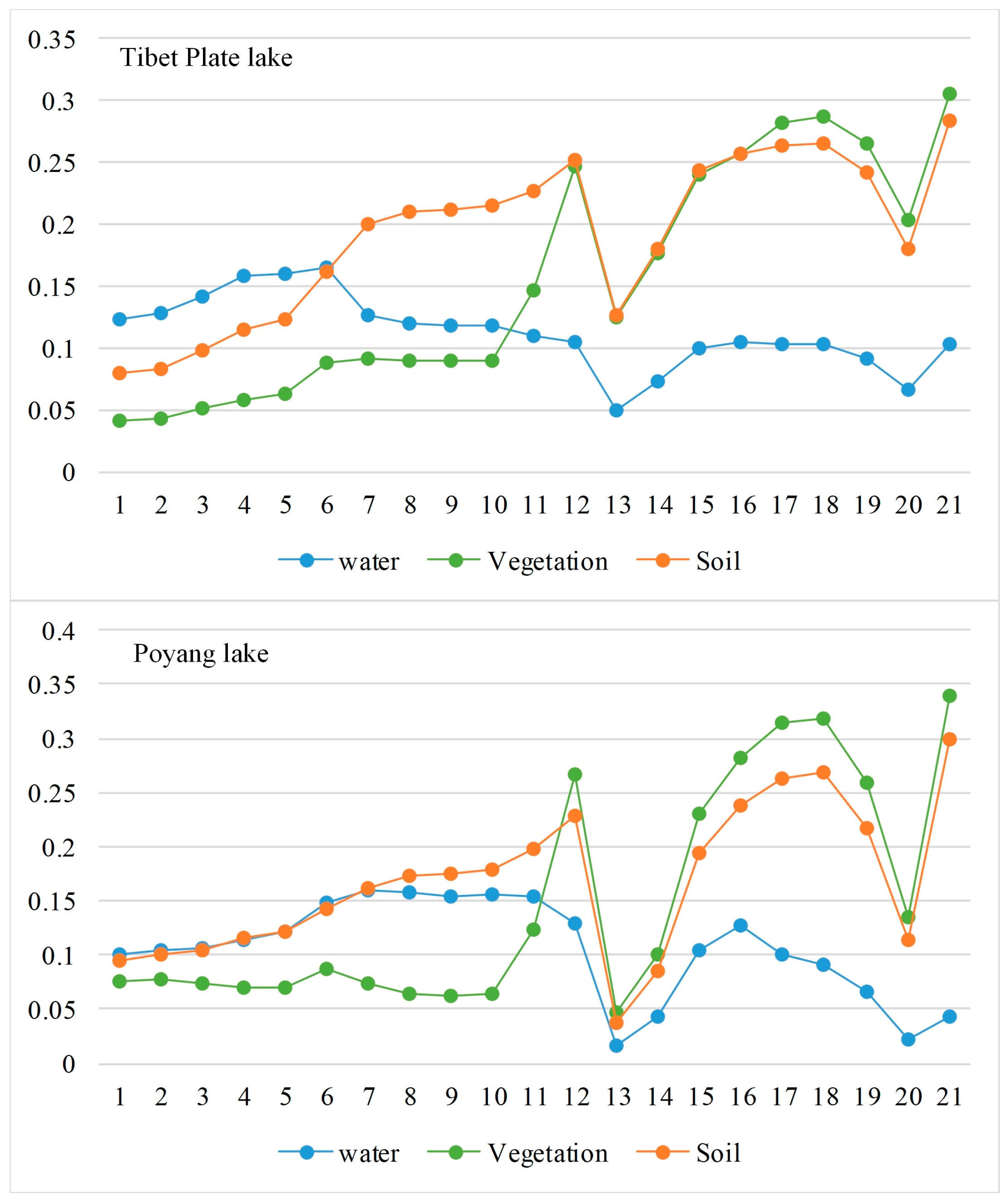
4.2. Spectral Response Analysis of Water Features

By randomly selecting samples of land cover classes of water, vegetation, and soil in the two Sentinel-3 OLCI images, Figure 4 reports the spectral response curves of three land covers in the Tibet Plate lake and Poyang lake. Because there are more bands in the Sentinel-3 OLCI image, the spectral curves for the three land covers are more continuous than those of many other satellite images, such as Landsat and MODIS images. As shown in Figure 3, it could be found that the classes of water, vegetation, and soil shares similar spectral curve trends in the two study sites. For the Tibet Plate lake, the vegetation and soil features had lower reflectance values than those of water from band 1 to 6, but higher reflectance from band 11 to 21. The reflectance value of water features had an increase from band 1 to 6, at this stage the water features were mainly expressed as a relatively high reflectance. Then, the reflectance of water had a rapid decrease from band 6 to 13 and an increase from band 13 to 17. For the NIR bands from 17 to 20, the reflectance had a slight decrease, but an increase was observed for band 21. The great fluctuations of water response may be because of the impurities mixed in the water of Tibet Plate lake.

Compared with water features in Tibet Plate lake, the spectral response curve of water in Poyang lake is more similar to that of the soil class. This indicates that the water in Poyang lake contained many soil types, and then the spectral response curves of water and soil classes share a similar trend. Particularly, from band 1 to 11, the water features of Poyang lake represented a relatively high reflectance, but the reflectance values decreased with the increase in wavelengths. From band 11 to 13, a rapid decrease of water reflectance value was observed, as the water features represented absorbance after band 11. By contrast, from band 13 to 16, an increase in reflectance could be seen; this is because bands 13–16 are sensitive to the mixed suspended matters including soil, sediment, and phytoplankton. For the NIR bands ranging from 17 to 20, the water absorbance became increasingly serious with the increase in wavelengths. In general, the water in most of the Tibet Plate lakes is clean and contains few impurities, but it is noteworthy that there would be many crystalline salts contained in the water in spring, which would make the water have a relatively high reflectance. In the water of Poyang lake, a lot of soil and sediment were mixed, and a relatively high reflectance could be observed. For Poyang lake, the difference between water and the two other land covers of vegetation and soil is not significant as the water features in the Tibet Plate lake, and thus the water bodies in Poyang lake would be more difficult to extract.

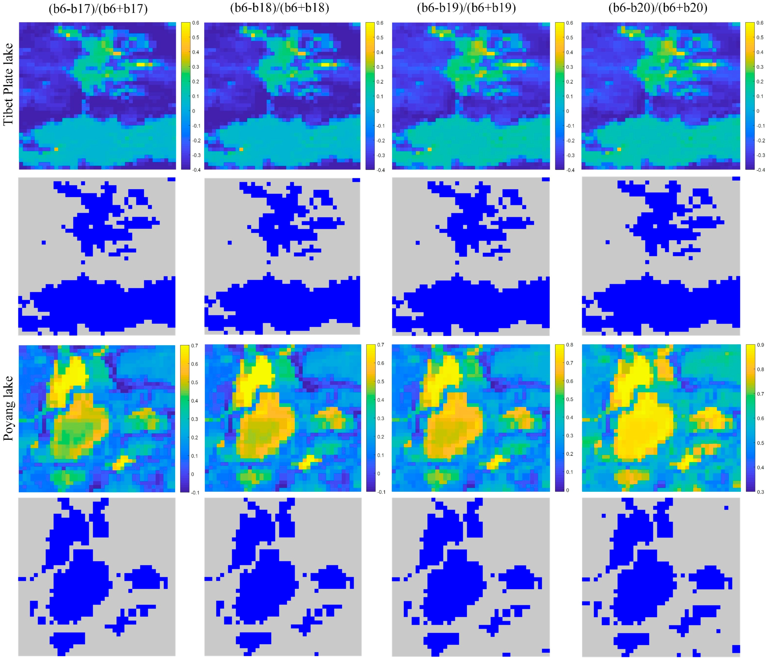
4.3. Pixel-Based Water Body Mapping from Different NDWI Images

For Sentinel-3 OLCI, although band 17 was always used as the NIR band to calculate the NDWI images, it is still possible for bands 18-20 to be considered as the NIR bands, as the wavelengths of bands 17–20 are too narrow. In this section, as shown in Figure 5, each of the bands 17–20 was used as the NIR band to calculate the NDWI images, and then OTSU segmentation algorithm was applied to the generated NDWI images to produce the pixel-based water body maps of Tibet Plate lake and Poyang lake.

Table 2. Accuracy assessment of the water body maps produced by OTSU segmentation with different NDWI images for Tibet Plate lake and Poyang lake.

	Water Index (NDWI)	Kappa	OA	Omission Error (Water)	Commission Error (Water)
Tibet plate lake	(b6-b17)/(b6+b17)	0.8166	91.07%	0.1166	0.0968
	(b6-b18)/(b6+b18)	0.8166	91.08%	0.1166	0.0968
	(b6-b19)/(b6+b19)	0.8166	91.08%	0.1166	0.0968
	(b6-b20)/(b6+b20)	0.8146	90.96%	0.1113	0.1035
Poyang lake	(b6-b17)/(b6+b17)	0.7106	87.73%	0.2077	0.1945
	(b6-b18)/(b6+b18)	0.7066	87.58%	0.2131	0.1950
	(b6-b19)/(b6+b19)	0.7038	87.43%	0.2106	0.2007
	(b6-b20)/(b6+b20)	0.6983	87.04%	0.1955	0.2192

reports the accuracy assessment of the water body maps produced by OTSU segmentation with different NDWI images. For Tibet Plate lake, although NDWI images based on bands 17, 18 and 19 had very similar accuracies (a slight increase was observed for bands 18 and 19), NDWI images based on band 20 achieved the worst accuracies. However, for the Poyang lake, the accuracy values of the NDWI images based on bands 17, 18, 19 and 20 had a continuous decrease. Based on a comparison of the performance of water body mapping with different NDWI images, it could be found that NDWI images based on the same bands would have very different results for different study sites; this is because water bodies at different study sites might have different reflectance features.

It is, therefore, difficult to guarantee that NDWI images based on one certain NIR band (e.g., band 17) would always achieve the best performance in water body mapping of Sentinel-3 OLCI image. The main reason behind this is that each of the wavelengths of the NIR bands 17–20 is too narrow, making it impossible for any NIR bands in Sentinel-3 OLCI image to contain enough spectral energy covering various water features. An alternative way is to use all four of the integrated NDWI images based on NIR bands 17–20 for water body mapping. With respect to this, the proposed USWBM method not only applies the widely used NDWI image based NIR band 17 as input, but also the other three NDWI images based on NIR bands 18–20 as input, so as to ensure USWBM could exploit most of the features of various water types and have a relatively stable performance.

4.4. Comparison of Water Body Mapping with Different Algorithms

With four NDWI images shown in Figure 5, USWBM produced fine spatial resolution (30 m) water body maps for the Tibet Plate lake and Poyang lake. Moreover, for comparison, the NDWI image based on the NIR band 17 and green band 6 was used as the input of OTSU segmentation and usFCM clustering to generate the 300 m spatial resolution water body maps. Four integrated NDWI images based on NIR bands 17–20 were also used as the input of the usFCM and usFCM_SPM algorithms to produce the 300 m and 30 m spatial resolution water body maps. Figure 6 and Figure 7 report the reference and resultant water body maps of different algorithms, and

Table 3. Accuracy assessment of the water body maps produced by different algorithms for Tibet Plate lake and Poyang lake.

		Coherence	Kappa	OA	Omission Error (Water)	Commission Error (Water)
Tibet plate lake	OSTU+NDWI	0.8167	0.8166	91.07%	0.1166	0.0968
	usFCM+NDWI	0.8174	0.8173	91.07%	0.1003	0.1098
	usFCM+4NDWI	0.8178	0.8178	91.09%	0.0973	0.1119
	usFCM_SPM+NDWI	0.8276	0.8273	91.61%	0.1153	0.0862
	usFCM_SPM+4NDWI	0.8329	0.8327	91.87%	0.1102	0.0847
	USWBM+4NDWI (δ = 0.004)	0.8387	0.8384	92.15%	0.1067	0.0810
	USWBM+4NDWI (δ = 0.012)	0.8432	0.8430	92.37%	0.1033	0.0795
Poyang lake	OSTU+NDWI	0.7106	0.7106	87.73%	0.2077	0.1945
	usFCM+NDWI	0.7106	0.7098	87.87%	0.2309	0.1755
	usFCM+4NDWI	0.7144	0.7114	88.12%	0.2541	0.1504
	usFCM_SPM+NDWI	0.7184	0.7181	88.12%	0.2129	0.1804
	usFCM_SPM+4NDWI	0.7209	0.7207	88.20%	0.2064	0.1826
	USWBM+4NDWI (δ = 0.004)	0.7265	0.7263	88.46%	0.20599	0.1757
	USWBM+4NDWI (δ = 0.012)	0.7345	0.7341	88.81%	0.2039	0.1672

lists the accuracy assessment of different results for Tibet Plate lake and Poyang lake. It is noteworthy that for the proposed USWBM algorithm, it will be the same as usFCM_SPM when the value of parameter $\delta$ is 0. In real applications, USWBM would produce any sub-pixel water body maps that usFCM_SPM can generate, and usFCM_SPM is a special case of USWBM.

For the Tibet Plate lake, it can be found that the OTSU segmentation and usFCM clustering can efficiently produce pixel-scale water body maps from the single NDWI image and integrated four NDWI images, but the boundaries of the results were jagged because both OTSU and usFCM are pixel-based methods and cannot deal with the mixed pixel problem around the boundaries. By contrast, for the result of usFCM_SPM (see Figure 6e) based on the single NDWI image, the boundaries became spatially smooth, and most of the water pixels in the result of usFCM_SPM were correctly mapped. For the result of usFCM_SPM (see Figure 6f) based on the four integrated NDWI images, it also produced a spatially smooth water body map. But because usFCM_SPM is only based on the sub-pixel based spatial dependence model, many pixels were locally over-smoothed and cannot maintain the overall structural information, where the boundaries are not smooth enough by comparing with the reference (as shown in the red ellipse). Although many small water patches were explored in the results of usFCM_SPM, most of them were not perfectly accurate and would have a negative impact on the accuracy. For the proposed USWBM algorithm (see Figure 6g,h), the boundaries were spatially smooth enough, which is the most similar to the reference water body map shown in Figure 6a, with particular for the result when $\delta$ was 0.012. This is because compared with the traditional usFCM_SPM, USWBM not only considers the sub-pixel based spatial dependence of water features, but also the coarse-pixel based water spatial dependence, which is important to maintain the integral structure information of water features.

For the Poyang lake shown in Figure 7, the OTSU segmentation and usFCM clustering produced water body maps with jagged boundaries. By contrast, usFCM_SPM can produce a much better water body map with spatially smooth boundaries, but many linear features of the water class were over-smooth and mapped as discontinuous patches. For the proposed USWBM algorithm, the boundaries are spatially smooth enough and many discontinuous patches were eliminated. As illustrated in the red ellipse, the results of USWBM contained better integral structure information of water features, especially when $\delta$ was 0.012.

Table 3 reports the accuracy assessment of the water body maps produced by different algorithms. For both of the study sites, the results of usFCM clustering achieved higher OA values than those of OTSU segmentation with one single NDWI image as input, especially for the Poyang lake. This stems from the fact that usFCM took into account the fractional information of water bodies during the clustering process. When the four NDWI images were used as the input of usFCM, better accuracy values were achieved by comparing with usFCM using single NDWI image as input, which demonstrates that it is more efficient to use integrated NDWI images to extract the water body map. Compared to the results of usFCM, usFCM_SPM produced a water body map with better accuracy values in the Tibet Plate lake and Poyang lake. Similarly, usFCM_SPM based on four integrated NDWI images also produced water body maps with better accuracies than those based on a single NDWI image. For the proposed USWBM algorithm, it produced a water body map with the highest Kappa and OA values and the smallest omission and commission error for both the Tibet Plate lake and Poyang lake when $\delta$ was 0.012. USWBM also achieved the largest coherence values, which indicate that it produced results that were the most similar to the reference water body maps. The following section will further discuss the effect of $\delta$ on the proposed algorithm.

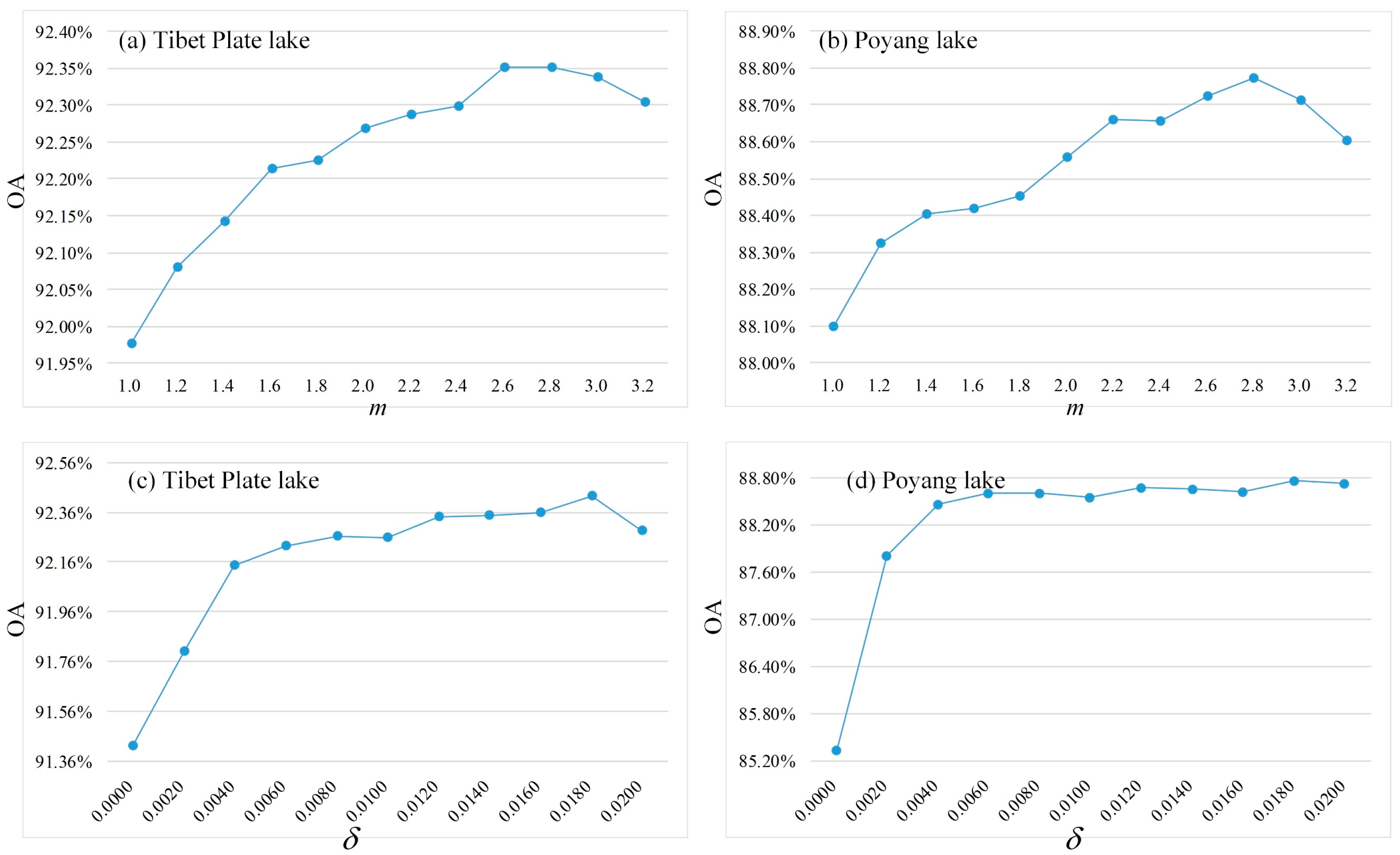
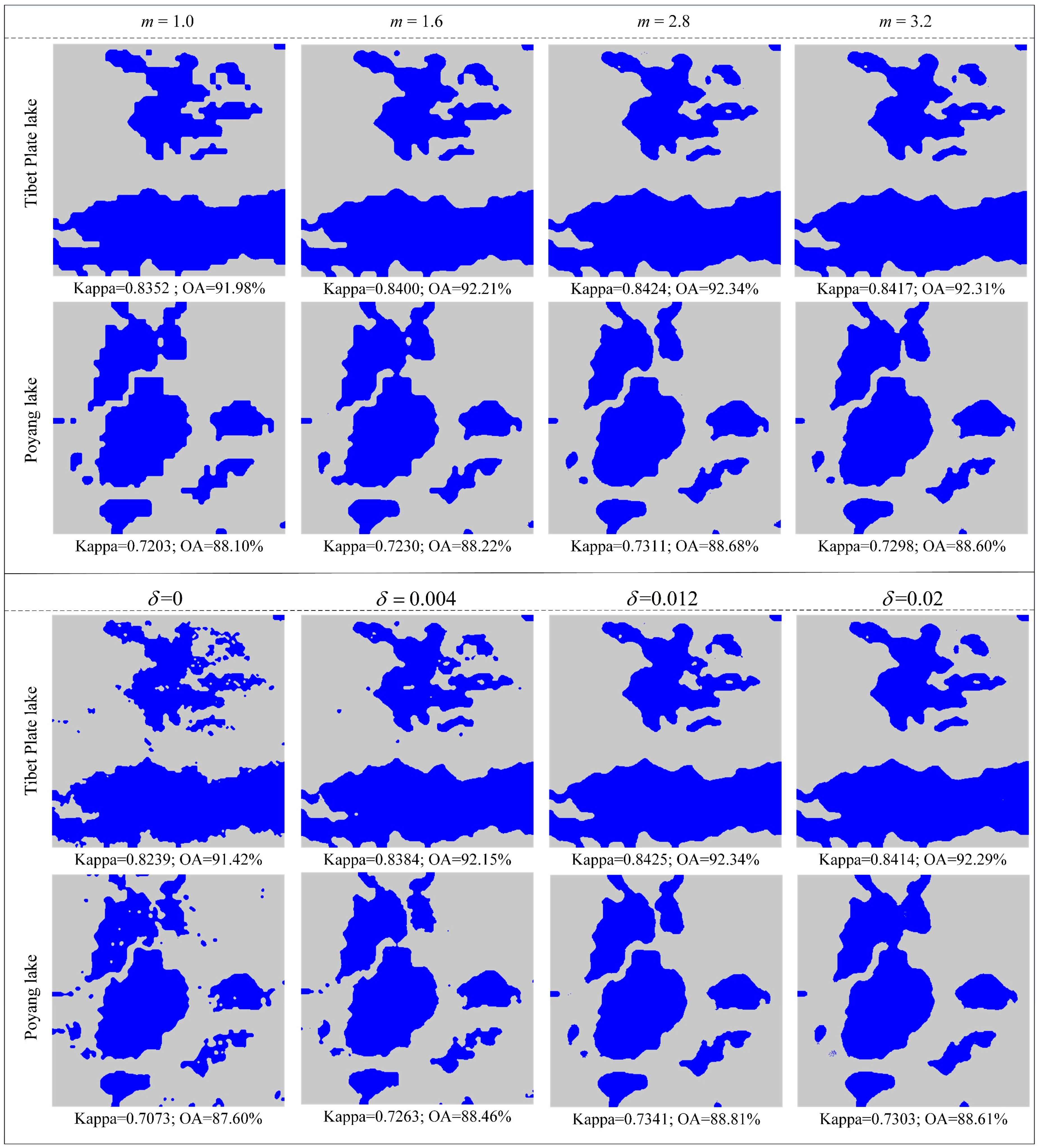
4.5. Effect of the Fuzziness Parameter and Coarse-Pixel Spatial Dependence

As the proposed USWBM algorithm is based on the unsupervised FCM clustering, the fuzziness parameter $m$ would have an important effect on the performance. Figure 8a,b report the curves of OA values for the resultant water body maps produced by USWBM with different values of $m$ for Tibet Plate lake and Poyang lake, and some results with different values of $m$ were also represented in Figure 9. For both of the two study sites, when $m$ was set to be 1.0, OA values of the results were the worst. Because the fraction value of water class in spectral water index term of USWBM can only be 1.0 when $m$ is equal to 1.0, and USWBM would be considered as a pixel-based method, this is also the reason why there are many jagged boundaries for resultant water body maps. However, with the increase in $m$, the OA values had a rapid increase, as the spectral water index term can provide accurate fraction values of the water class, and the boundaries became spatially smooth when $m$ was equal to 1.6 and 2.8. By contrast, if the value of $m$ is set too large, OA values of the resultant water body maps could not increase, or may even decrease. Some isolated small-sized patches would appear around the boundaries, as shown in Figure 9 when $m$ was equal to 3.2, especially for the result of Poyang lake.

In addition, the coarse-pixel spatial dependence is important for the performance of USWBM, and it is urgent to have a quantitative validation of the influence of parameter $\delta$, as it controls the contribution of coarse-pixel spatial dependence. Figure 8c,d reports the curves of OA values and Figure 9 lists some results of USWBM with different values of $\delta$. When $\delta$ was equal to 0, many isolated over-smoothed patches were found around the boundaries. The boundaries become more spatially smooth when $\delta$ was equal to 0.004 and 0.012. But when $\delta$ was equal to 0.02, the water features in the two study areas were over-smoothed; many linear water features were interrupted in Tibet Plate lake, while many separate patches were mapped together in the Poyang lake, which indicates that $\delta$ was set too large.

4.6. Advantages, Error Sources and Future Work

Mapping natural water surfaces is always a challenging task, as the open water surface in some places, such as the study site of Poyang lake, would have a serious change during a short time. In order to monitor the timely change of water surface, it always requires that satellite images have a very fine temporal resolution. Similar to the MERIS and MODIS images, the Sentinel-3 OLCI image has a great advantage of fine temporal resolution, but its spatial resolution is often too coarse. With respect to this, USWBM was proposed to produce fine spatial and temporal resolution water body maps. In summary, USWBM holds the following key advantages in water body mapping:

(1)

Compared with the traditional pixel-based water body mapping methods, USWBM can extract water body maps from Sentinel-3 OLCI image at the sub-pixel scale.

(2)

Compared with the traditional sub-pixel water body mapping methods, USWBM can directly extract water body map from NDWI images, and there is no need for USWBM to collect training samples and endmembers of water and non-water classes.

(3)

Compared with the traditional unsupervised sub-pixel mapping method of usFCM_SPM, USWBM takes into account the coarse-pixel spatial dependence of water features, so as to provide holistic information of water class. Moreover, USWBM would produce any sub-pixel water body maps that usFCM_SPM can generate, and usFCM_SPM is a special case of USWBM.

Although USWBM has many advantages in sub-pixel water body mapping from Sentinel-3 OLCI image, the resultant water body maps are limited to provide spatial details of some water features, such as linear features and small-sized patches shown in the reference water body maps (see Figure 6 and Figure 7). It is noted that exploring small-sized land cover features is always a challenging problem in the field of SPM, especially when the spatial scale is large (e.g., 10 in this research) [50]. On the one hand, although most of the spatial distribution of nature water surface is consistent with the maximal spatial dependence principle, the spatial patterns of many small-sized water features are often spatial heterogeneity, which could make it challenging for the proposed USWBM algorithm to exploit some small-sized water features. On the other hand, small-sized water features always have similar spatial structures as those of noise patches caused by the spectral water index term [40]. If we want to maintain the small-sized water features in the results, the noise patches would be introduced unavoidably; but when we want to eliminate the noise patches, the small-sized water patches would also be removed. Meanwhile, due to the coarse spatial resolution of Sentinel-3 OLCI image, it is difficult to control the coordinate transformation and registration errors, which would make the small-sized water patches locate in the wrong place in the result.

In future work, there are three aspects could be focused to overcome the abovementioned shortcoming. First, instead of only using the maximal spatial dependence principle to allocate the spatial distribution of water class, some example-based SPM methods [51] can be used to learn various spatial patterns of water features, especially for the small-sized spatial patterns. Second, as the spatial distribution of water surface is highly relevant to the digital elevation models (DEM), prior information based on DEM can be added into the USWBM method to explore more accurate small-sized patches in the resultant water body map [32]. Third, for most of the study sites, there are always some previous fine spatial resolution satellite images (such as Landsat and SPOT images) in real applications; these existing previous fine spatial resolution satellite images can be used to provide prior temporal information about water features for the water body map produced by USWBM from Sentinel-3 OLCI image at the predicted time [52,53].

5. Conclusions

The newly launched Sentinel-3 OLCI image has 21 bands covering from visible to near-infrared and has a fine temporal resolution of nearly 2 days with a double satellites system, which makes it possible to provide near real-time water body monitoring. However, the spatial resolution of Sentinel-3 OLCI image is limited to 300 m, which may include lots of mixed pixels around the boundaries of water bodies. In order to promote the application of Sentinel-3 OLCI in the field of water body mapping, an unsupervised SPM method (USWBM) was proposed particularly in this paper to produce a finer spatial resolution water body map from Sentinel-3 OLCI image. Four integrated NDWI images extracted from the NIR bands 17–20 and green band 6 of Sentinel-3 OLCI image were used as the input data to directly produce sub-pixel water body maps, so as to ensure the proposed USWBM algorithm can achieve a stable performance for different types of water features. Moreover, USWBM not only considers the sub-pixel based spatial dependence of water features, but also the coarse-pixel-based water spatial dependence. From the experiments at Tibet Plate lake and Poyang lake, it could be found that it is difficult to guarantee that NDWI images based on one certain NIR band (e.g., band 17) would always produce the best pixel-scale water body map. Compared the pixel-scale water body mapping methods (e.g., OTSU and usFCM), the sub-pixel results produced by usFCM_SPM and USWBM were more spatially smooth and contained more spatial detail about various water features. usFCM_SPM always produced sub-pixel water body maps with many small-sized patches, but many of them are not perfectly accurate. Compared with usFCM_SPM, the results of USWBM had larger coherence with the reference water body maps and were able to maintain the integral structure information of water features. However, many small-sized water features were also lost in the results of USWBM. In future work, prior information about the spatial distributions of water features is of great interest to be integrated into the USWBM model to further improve the performance. Moreover, as the performance of USWBM is sensitive to the values of different parameters, further research will also focus on the parameter value selection and automatic estimation.

References

1. Tolpekin, V.A.; Stein, A. Quantification of the effects of Land-Cover-Class spectral separability on the accuracy of markov-Random-Field-Based superresolution mapping. IEEE Trans. Geosci. Remote. Sens. 2009, 47, 3283–3297. [Google Scholar] [CrossRef]
2. Woerd, H.; Wernand, M. True colour classification of natural waters with medium-spectral resolution satellites: SeaWiFS, MODIS, MERIS and OLCI. Sensors 2015, 15, 25663–25680. [Google Scholar] [CrossRef] [PubMed]
3. Toming, K.; Kutser, T.; Uiboupin, R.; Arikas, A.; Vahter, K.; Paavel, B. Mapping water quality parameters with Sentinel-3 ocean and land colour instrument imagery in the Baltic Sea. Remote Sens. 2017, 9, 1070. [Google Scholar] [CrossRef]
4. Wang, Q.; Atkinson, P.M. Spatio-temporal fusion for daily sentinel-2 images. Remote Sens. Environ. 2018, 204, 31–42. [Google Scholar] [CrossRef]
5. Berger, M.; Moreno, J.; Johannessen, J.A.; Levelt, P.F.; Hanssen, R.F. ESA’s sentinel missions in support of Earth system science. Remote Sens. Environ. 2012, 120, 84–90. [Google Scholar] [CrossRef]
6. Donlon, C.; Berruti, B.; Buongiorno, A.; Ferreira, M.H.; Féménias, P.; Frerick, J.; Goryl, P.; Klein, U.; Laur, H.; Mavrocordatos, C.; et al. The global monitoring for environment and security (GMES) Sentinel-3 mission. Remote Sens. Environ. 2012, 120, 37–57. [Google Scholar] [CrossRef]
7. Verrelst, J.; Muñoz, J.; Alonso, L.; Delegido, J.; Rivera, J.P.; Camps-Valls, G.; Moreno, J. Machine learning regression algorithms for biophysical parameter retrieval: Opportunities for Sentinel-2 and -3. Remote Sens. Environ. 2012, 118, 127–139. [Google Scholar] [CrossRef]
8. Clevers, J.G.P.W.; Gitelson, A.A. Remote estimation of crop and grass chlorophyll and nitrogen content using red-edge bands on Sentinel-2 and -3. Int. J. Appl. Earth Obs. 2013, 23, 344–351. [Google Scholar] [CrossRef]
9. Nguy-Robertson, A.L.; Gitelson, A.A. Algorithms for estimating green leaf area index in C3 and C4 crops for MODIS, Landsat TM/ETM+, MERIS, Sentinel MSI/OLCI, and Venµs sensors. Remote Sens. Lett. 2015, 6, 360–369. [Google Scholar] [CrossRef]
10. Shen, M.; Duan, H.; Cao, Z.; Xue, K.; Loiselle, S.; Yesou, H. Determination of the downwelling diffuse attenuation coefficient of lake water with the Sentinel-3A OLCI. Remote Sens. 2017, 9, 1246. [Google Scholar] [CrossRef]
11. Ruescas, A.; Hieronymi, M.; Mateo-Garcia, G.; Koponen, S.; Kallio, K.; Camps-Valls, G. Machine learning regression approaches for colored dissolved organic matter (CDOM) retrieval with S2-MSI and S3-OLCI simulated data. Remote Sens. 2018, 10, 786. [Google Scholar] [CrossRef]
12. Schiller, H.; Doerffer, R. Improved determination of coastal water constituent concentrations from MERIS data. IEEE Trans. Geosci. Remote. Sens. 2005, 43, 1585–1591. [Google Scholar] [CrossRef]
13. Carroll, M.L.; Townshend, J.R.; Dimiceli, C.M.; Noojipady, P.; Sohlberg, R.A. A new global raster water mask at 250 m resolution. Int. J. Digit. Earth 2009, 2, 291–308. [Google Scholar] [CrossRef] [Green Version]
14. Feng, L.; Hu, C.; Chen, X.; Cai, X.; Tian, L.; Gan, W. Assessment of inundation changes of Poyang Lake using MODIS observations between 2000 and 2010. Remote Sens. Environ. 2012, 121, 80–92. [Google Scholar] [CrossRef]
15. Ge, X.; Sun, X.; Liu, Z. Object-oriented coastline classification and extraction from remote sensing imagery. Remote Sens. Environ. 2014, 140, 704–716. [Google Scholar]
16. Li, S.; Sun, D.; Goldberg, M.; Stefanidis, A. Derivation of 30-m-resolution water maps from TERRA/MODIS and SRTM. Remote Sens. Environ. 2013, 134, 417–430. [Google Scholar] [CrossRef]
17. Majozi, N.P.; Salama, M.S.; Bernard, S.; Harper, D.M.; Habte, M.G. Remote sensing of euphotic depth in shallow tropical inland waters of Lake Naivasha using MERIS data. Remote Sens. Environ. 2014, 148, 178–189. [Google Scholar] [CrossRef]
18. Zurita-Milla, R.; Gomez-Chova, L.; Guanter, L.; Clevers, J.G.P.W.; Camps-Valls, G. Multitemporal unmixing of medium-spatial-resolution satellite images: A case study using MERIS images for land-cover mapping. IEEE Trans. Geosci. Remote. Sens. 2011, 49, 4308–4317. [Google Scholar] [CrossRef]
19. Carrão, H.; Araujo, A.; Gonçalves, P.; Caetano, M. Multitemporal MERIS images for land-cover mapping at a national scale: A case study of Portugal. Int. J. Remote Sens. 2010, 31, 2063–2082. [Google Scholar] [CrossRef]
20. Work, E.A., Jr.; Gilmer, D.S. Utilization of satellite data for inventorying prairie ponds and lakes. Photogramm. Eng. Remote Sens. 1976, 42, 685–694. [Google Scholar]
21. Sun, D.; Yu, Y.; Goldberg, M.D. Deriving water fraction and flood maps from MODIS images using a decision tree approach. IEEE J. STARS 2011, 4, 814–825. [Google Scholar] [CrossRef]
22. Crasto, N.; Hopkinson, C.; Forbes, D.L.; Lesack, L.; Marsh, P.; Spooner, I.; Van Der Sanden, J.J. A LiDAR-based decision-tree classification of open water surfaces in an Arctic delta. Remote Sens. Environ. 2015, 164, 90–102. [Google Scholar] [CrossRef]
23. Franke, J.; Roberts, D.A.; Halligan, K.; Menz, G. Hierarchical Multiple Endmember Spectral Mixture Analysis (MESMA) of hyperspectral imagery for urban environments. Remote Sens. Environ. 2009, 113, 1712–1723. [Google Scholar] [CrossRef]
24. Du, Y.; Zhang, Y.; Ling, F.; Wang, Q.; Li, W.; Li, X. Water bodies’ mapping from sentinel-2 imagery with modified normalized difference water index at 10-m spatial resolution produced by sharpening the SWIR band. Remote Sens. 2016, 8, 354. [Google Scholar] [CrossRef]
25. Li, W.; Du, Z.; Ling, F.; Zhou, D.; Wang, H.; Gui, Y.; Sun, B.; Zhang, X. A comparison of land surface water mapping using the normalized difference water index from TM, ETM+ and ALI. Remote Sens. 2013, 5, 5530–5549. [Google Scholar] [CrossRef]
26. Mcfeeters, S.K. The use of the normalized difference water index (NDWI) in the delineation of open water features. Int. J. Remote Sens. 1996, 17, 1425–1432. [Google Scholar] [CrossRef]
27. Xu, H. Modification of normalised difference water index (NDWI) to enhance open water features in remotely sensed imagery. Int. J. Remote Sens. 2006, 27, 3025–3033. [Google Scholar] [CrossRef]
28. Feyisa, G.L.; Meilby, H.; Fensholt, R.; Proud, S.R. Automated water extraction index: A new technique for surface water mapping using Landsat imagery. Remote Sens. Environ. 2014, 140, 23–35. [Google Scholar] [CrossRef]
29. Kasetkasem, T.; Arora, M.K.; Varshney, P.K. Super-resolution land cover mapping using a Markov random field based approach. Remote Sens. Environ. 2005, 96, 302–314. [Google Scholar] [CrossRef]
30. Atkinson, P.M. Sub-pixel target mapping from soft-classified, remotely sensed imagery. Photogramm. Eng. Remote Sens. 2005, 71, 839–846. [Google Scholar] [CrossRef]
31. Foody, G.M. Sharpening fuzzy classification output to refine the representation of sub-pixel land cover distribution. Int. J. Remote Sens. 1998, 19, 2593–2599. [Google Scholar] [CrossRef]
32. Ling, F.; Xiao, F.; Du, Y.; Xue, H.P.; Ren, X.Y. Waterline mapping at the subpixel scale from remote sensing imagery with high-resolution digital elevation models. Int. J. Remote Sens. 2008, 29, 1809–1815. [Google Scholar] [CrossRef]
33. Muad, A.M.; Foody, G.M. Super-resolution mapping of lakes from imagery with a coarse spatial and fine temporal resolution. Int. J. Appl. Earth Obs. 2012, 15, 79–91. [Google Scholar] [CrossRef]
34. Huang, C.; Chen, Y.; Wu, J. DEM-based modification of pixel-swapping algorithm for enhancing floodplain inundation mapping. Int. J. Remote Sens. 2014, 35, 365–381. [Google Scholar] [CrossRef]
35. Li, L.; Chen, Y.; Yu, X.; Liu, R.; Huang, C. Sub-pixel flood inundation mapping from multispectral remotely sensed images based on discrete particle swarm optimization. ISPRS J. Photogramm. Remote Sens. 2015, 101, 10–21. [Google Scholar] [CrossRef]
36. Li, L.; Chen, Y.; Xu, T.; Liu, R.; Shi, K.; Huang, C. Super-resolution mapping of wetland inundation from remote sensing imagery based on integration of back-propagation neural network and genetic algorithm. Remote Sens. Environ. 2015, 164, 142–154. [Google Scholar] [CrossRef]
37. Li, W.; Zhang, X.; Ling, F.; Zheng, D. Locally adaptive super-resolution waterline mapping with MODIS imagery. Remote Sens. Lett. 2016, 7, 1121–1130. [Google Scholar] [CrossRef]
38. Huang, W.; Devries, B.; Huang, C.; Lang, M.W.; Jones, J.W.; Creed, I.F.; Carroll, M. Automated extraction of surface water extent from Sentinel-1 data. Remote Sens. 2018, 10, 797. [Google Scholar] [CrossRef]
39. Li, S.; Sun, D.; Goldberg, M.D.; Sjoberg, B.; Santek, D.A.; Hoffman, J.P.; Deweese, M.; Restrepo, P.; Lindsey, S.; Holloway, E. Automatic near real-time flood detection using Suomi-NPP/VIIRS data. Remote Sens. Environ. 2018, 204, 672–689. [Google Scholar] [CrossRef]
40. Zhang, Y.; Du, Y.; Li, X.; Fang, S.; Ling, F. Unsupervised subpixel mapping of remotely sensed imagery based on fuzzy C-means clustering approach. IEEE Geosci. Remote Sens. 2014, 11, 1024–1028. [Google Scholar] [CrossRef]
41. Zhang, Y.; Du, Y.; Ling, F.; Wang, X.; Li, X. Spectral–spatial based sub-pixel mapping of remotely sensed imagery with multi-scale spatial dependence. Int. J. Remote Sens. 2015, 36, 2831–2850. [Google Scholar] [CrossRef]
42. Wang, Q.; Shi, W.; Atkinson, P.M. Sub-pixel mapping of remote sensing images based on radial basis function interpolation. ISPRS J. Photogramm. Remote Sens. 2014, 92, 1–15. [Google Scholar] [CrossRef]
43. Wang, X.; Liu, Y.; Ling, F.; Xu, S. Fine spatial resolution coastline extracting from Landsat-8 OLI imagery by integrating downscaling and pansharpening approaches. Remote Sens. Lett. 2018, 9, 314–323. [Google Scholar] [CrossRef]
44. Keshava, N.; Mustard, J.F. Spectral Unmixing. IEEE Signal Proc. Mag. 2002, 19, 44–57. [Google Scholar] [CrossRef]
45. Atkinson, P.M. Mapping sub-pixel vector boundaries from remotely sensed images. Innov. GIS 1997, 4, 166–180. [Google Scholar]
46. Tatem, A.J.; Lewis, H.G.; Atkinson, P.M.; Nixon, M.S. Super-resolution land cover pattern prediction using a Hopfield neural network. Remote Sens. Environ. 2002, 79, 1–14. [Google Scholar] [CrossRef] [Green Version]
47. Foody, G.M.; Cox, D.P. Sub-pixel land cover composition estimation using a linear mixture model and fuzzy membership functions. Int. J. Remote Sens. 1994, 15, 619–631. [Google Scholar] [CrossRef]
48. Lin, K.C. On improvement of the computation speed of Otsu’s image thresholding. J. Electron. Imaging 2005, 14, 023011. [Google Scholar] [CrossRef]
49. Lim, Y.W.; Lee, S.U. On the color image segmentation algorithm based on the thresholding and the fuzzy C-means techniques. Pattern Recogn. 1990, 23, 935–952. [Google Scholar]
50. Atkinson, P.M. Downscaling in remote sensing. Int. J. Appl. Earth Obs. 2013, 22, 106–114. [Google Scholar] [CrossRef]
51. Zhang, Y.; Du, Y.; Ling, F.; Fang, S.; Li, X. Example-Based Super-Resolution Land Cover Mapping Using Support Vector Regression. IEEE J. STARS 2014, 7, 1271–1283. [Google Scholar] [CrossRef]
52. Ling, F.; Li, W.; Du, Y.; Li, X. Land cover change mapping at the subpixel scale with different spatial-resolution remotely sensed imagery. IEEE Geosci. Remote Sens. 2011, 8, 182–186. [Google Scholar] [CrossRef]
53. Li, X.; Ling, F.; Foody, G.M.; Ge, Y.; Zhang, Y.; Du, Y. Generating a series of fine spatial and temporal resolution land cover maps by fusing coarse spatial resolution remotely sensed images and fine spatial resolution land cover maps. Remote Sens. Environ. 2017, 196, 293–311. [Google Scholar] [CrossRef] [Green Version]
Figure 1. Illustration of sub-pixel water body mapping from Sentinel-3 OLCI image.
Remotesensing 11 00327 g001
Figure 2. Flowchart of the proposed USWBM approach.
Remotesensing 11 00327 g002
Figure 3. Sentinel-3A (RGB20-10-5) OLIC image, Landsat-8 (RGB5-4-3) multi-spectral image and reference water body maps for the Tibet Plate lake and Poyang lake.
Remotesensing 11 00327 g003
Figure 4. Spectral response curves of water, vegetation, and soil in the Sentinel-3 OLCI image for the Tibet Plate lake and Poyang lake.
Remotesensing 11 00327 g004
Figure 5. NDWI images based on NIR bands of 17, 18, 19 and 20, and corresponding water body maps generated by OTSU segmentation.
Remotesensing 11 00327 g005
Figure 6. Water body maps generated by different algorithms for Tibet Plate lake. (a) Reference water body map; (b) Water body map produced from the NDWI image (based on NIR band 17) by using OSTU segmentation; (c) Water body map produced from the NDWI image by using usFCM segmentation; (d) Water body map produced from the four integrated NDWI images by using usFCM segmentation; (e) Water body map produced from the NDWI images by using usFCM_SPM segmentation; (f) Water body map produced from the four integrated NDWI images by using usFCM_SPM segmentation; (g,h) Water body map produced from the four integrated NDWI images by using the proposed USWBM algorithm when δ was 0.004 and 0.012, respectively.
Remotesensing 11 00327 g006
Figure 7. Water body maps generated by different algorithms for the Poyang lake. (a) Reference water body map; (b) Water body map produced from the NDWI image (based on NIR band 17) by using OSTU segmentation; (c) Water body map produced from the NDWI image by using usFCM segmentation; (d) Water body map produced from the four integrated NDWI images by using usFCM segmentation; (e) Water body map produced from the NDWI images by using usFCM_SPM segmentation; (f) Water body map produced from the four integrated NDWI images by using usFCM_SPM segmentation; (g,h) Water body map produced from the four integrated NDWI images by using the proposed USWBM algorithm when δ was 0.004 and 0.012, respectively.
Remotesensing 11 00327 g007
Figure 8. OA curves of the resultant water body maps produced by USWBM with different values of m and δ for Tibet Plate lake and Poyang lake. (a) OA curves of the results in Tibet plate lake with different values of m, (b) OA curves of the results in Poyang lake with different values of m, (c) OA curves of the results in Tibet plate lake with different values of δ, (d) OA curves of the results in Tibet plate lake with different values of δ.
Remotesensing 11 00327 g008
Figure 9. Resultant water body maps of USWBM with different values of m and δ.
Remotesensing 11 00327 g009