Article

Hierarchical Clustering-Aligning Framework Based Fast Large-Scale 3D Reconstruction Using Aerial Imagery

1
National Engineering Laboratory for Integrated Aero-Space-Ground-Ocean Big Data Application Technology, School of Computer Science and Engineering, Northwestern Polytechnical University, Xi’an 710071, China
2
Research & Development Institute of Northwestern Polytechnical University in Shenzhen, Shenzhen 518057, China
*
Authors to whom correspondence should be addressed.
Remote Sens. 2019, 11(3), 315; https://doi.org/10.3390/rs11030315
Submission received: 22 December 2018 / Revised: 25 January 2019 / Accepted: 2 February 2019 / Published: 5 February 2019
(This article belongs to the Special Issue 3D Reconstruction Based on Aerial and Satellite Imagery)

Abstract

:
With extensive applications of Unmanned Aircraft Vehicle (UAV) in the field of remote sensing, 3D reconstruction using aerial images has been a vibrant area of research. However, fast large-scale 3D reconstruction is a challenging task. For aerial image datasets, large scale means that the number and resolution of images are enormous, which brings significant computational cost to the 3D reconstruction, especially in the process of Structure from Motion (SfM). In this paper, for fast large-scale SfM, we propose a clustering-aligning framework that hierarchically merges partial structures to reconstruct the full scene. Through image clustering, an overlapping relationship between image subsets is established. With the overlapping relationship, we propose a similarity transformation estimation method based on joint camera poses of common images. Finally, we introduce the closed-loop constraint and propose a similarity transformation-based hybrid optimization method to make the merged complete scene seamless. The advantage of the proposed method is a significant efficiency improvement without a marginal loss in accuracy. Experimental results on the Qinling dataset captured over Qinling mountain covering 57 square kilometers demonstrate the efficiency and robustness of the proposed method.

1. Introduction

With the development of Unmanned Aircraft Vehicle (UAV), low-altitude remote sensing is playing an increasingly important role in land cover monitoring [1,2,3], heritage site protection [4], and vegetation observation [5,6,7]. For these applications, aerial imagery-based 3D reconstruction of large-scale scenes is highly desired. For instance, Mancini et al. [1] used 3D reconstruction from UAV images to get accurate topographic information for coastal geomorphology, which could be used to perform a reliable simulation of coastal erosion and flooding phenomena.
Structure from Motion (SfM) is a 3D reconstruction method used to recover the 3D structure of stationary scenes from a set of projective measurements, via motion estimation of the cameras corresponding to images. In essence, SfM involves the three main stages of: (1) extraction of features in images (i.e., points of interest) and matching these features between images; (2) camera motion estimation (i.e., camera poses including the rotation matrix and translation vector); and (3) recovery of the 3D structure using the estimated motion and features. Among the 3D reconstruction methods, SfM is a basic 3D reconstruction approach that is able to recover sparse 3D information and camera motion parameters from images, which is the basis for generating successively-dense point clouds and high-resolution Digital Surface Models (DSMs). Therefore, SfM is the primary task for the research and application of 3D reconstruction using aerial images.
However, the application of SfM technology to large-scale 3D reconstruction is a very challenging task because of the efficiency problem. For SfM, large-scale means that there is a larger range of scenes to be reconstructed. Obviously, in order to reconstruct the large-scale scene structure, more aerial images and greater image resolution are required, which brings a computational challenge for each step of the SfM pipeline, such as feature matching. For example, given a dataset with n images, this will result in n ( n 1 ) / 2 possible image pairs, hence leading to O( n 2 ) complexity for feature matching. On the other hand, the number of features detected from large resolution images is generally very high. Consequently, the computational cost of feature matching is adequately huge, which constrains the efficiency of reconstruction.
Strategies for SfM can be divided into two main classes: incremental [8,9] and global [10,11,12]. Incremental SfM pipelines start from a minimum reconstruction based on two views and then incrementally add new views to a merged model. During the adding image process, periodic Bundle Adjustment (BA) [13] is required to optimize the 3D points of the scene structure and camera poses. The essence of BA is an optimization process, the purpose of which is to minimize the re-projection error. Re-projection error is obtained by comparing the pixel coordinates (i.e., the observed feature positions) with the 2D positions projected by 3D points according to the camera pose of the projected image. Incremental methods are generally slow. This is mainly because of the exhaustive feature matching in a large number of image pairs. In addition, periodic global BA is time consuming. As for global pipelines, most are solved in two steps. The first step estimates the global rotation of each view, and the second step estimates the camera translations and the scene structure. Although global SfM avoids periodic global BA, it still encounters the computational bottleneck brought by feature matching in a large number of image pairs. In other words, both strategies aim at entire image sets, thus causing a serious efficiency problem for large-scale SfM.
To tackle the efficiency problem for large-scale SfM, researchers have proposed some solutions. Some researchers have focused on the BA optimization problem for large-scale SfM. For large-scale SfM, there is a huge number of reconstructed 3D points and camera parameters. Therefore, the global BA optimization of all 3D points and camera parameters is a slow process. Steedly et al. [14] proposed a spectral partitioning approach for large-scale optimization problems, specifically structure from motion. The idea is to decompose the optimization problem into smaller, more tractable components. The subproblems can be selected using the Hessian of the reprojection error and its eigenvectors. Ni et al. [15] presented an out-of-core bundle adjustment algorithm, in which the original problem is decoupled into several submaps that have their own local coordinate systems and can be optimized in parallel. However, this method only focuses on the last step of reconstruction, and the solution to the efficiency problem is limited. Obviously, the decomposition of the SfM problem from the beginning of the reconstruction pipeline can maximize the efficiency of reconstruction. Some researchers exploited a simplified graph of iconic images. Frahm et al. [16] first obtained a set of canonical views by clustering the gist features and then established a skeleton and extended it using registration. Shah et al. [17] proposed a multistage approach for SfM that involves first reconstructing a coarse global model using a match-graph of a few features and enriching it later by simultaneously localizing additional images and triangulating additional points. These methods merge multiple sub-models by finding the common 3D points across the models. However, 3D point matches obtained by 2–3D correspondences and 2D feature matching are contaminated by outliers, especially in repetitive structure scenes. Thus, care must be taken to identify common 3D points. Some researchers [18,19,20,21] have organized a hierarchical tree and merged partial reconstructions along the tree. However, the merging processes still rely on 3D point matches to estimate similarity transformations. Some researchers have proposed novel merging methods that do not depend on 3D matches. Bhowmick et al. [22] estimated the similarity transformation between two models by leveraging the pairwise epipolar geometry of the link images. Sweeney et al. [23] introduced a distributed camera model, which represents partial reconstructions as distributed cameras, and incrementally merges distributed cameras by solving a generalized absolute pose and scale problem. However, these methods that incrementally merge partial reconstructions may suffer from drifting errors.
To address all of these problems, in this paper, we propose a novel method for fast, large-scale SfM. The contributions of this work are as follows:
  • First, we present a clustering-aligning framework to perform fast 3D reconstruction. Clustering refers to the clustering of images to obtain the associated image subsets. This specific image organization lays a foundation for the subsequent partial reconstruction alignment.
  • Second, in the process of aligning partial reconstructions, we present a robust initial similarity transformation estimation method based on joint camera poses of common images across image subsets without 3D point matches.
  • Third, we present a similarity transformation-based BA hybrid optimization method to make the merged scene structure seamless. In the process of similarity transformation optimization, we introduce closed-loop constraints.
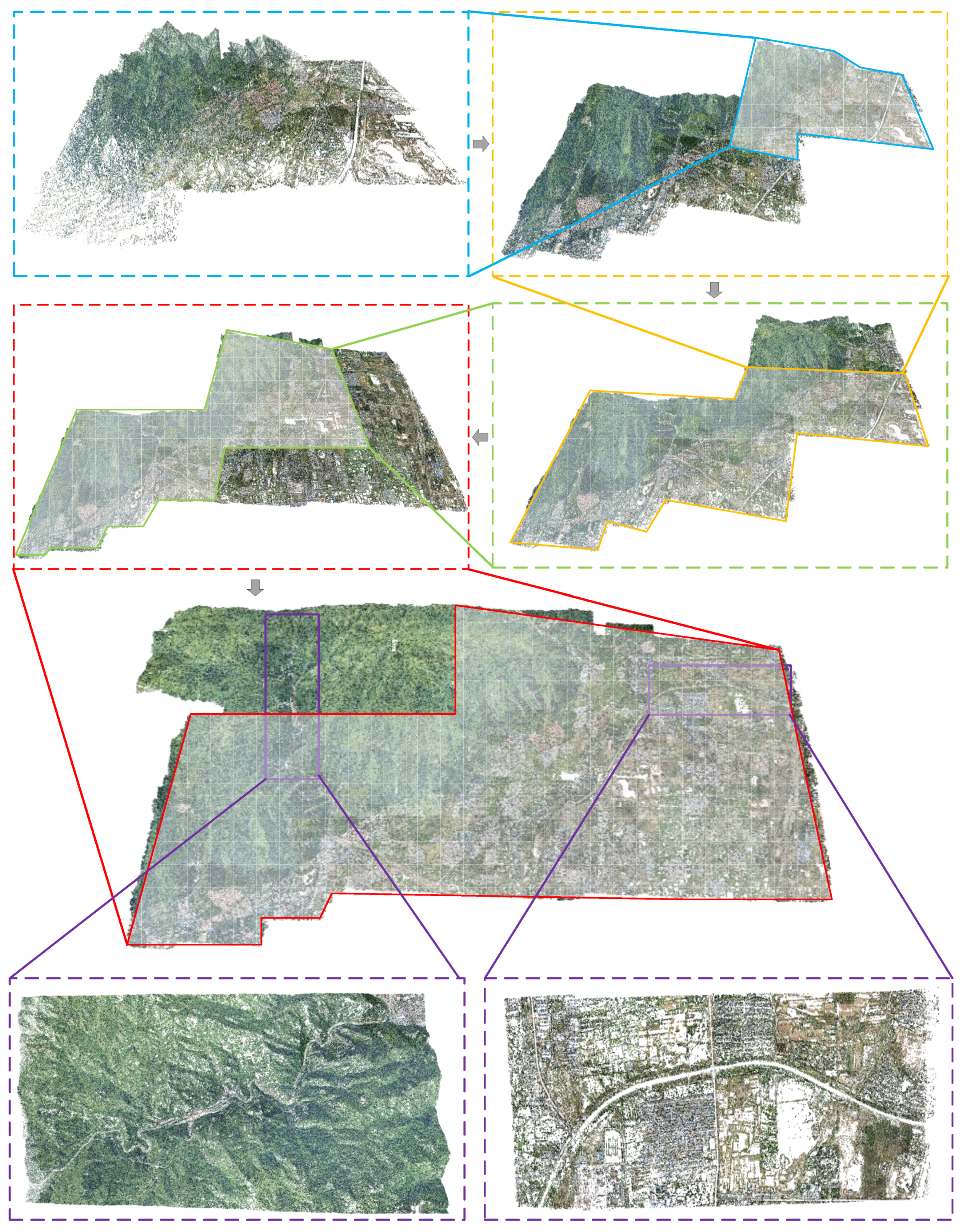
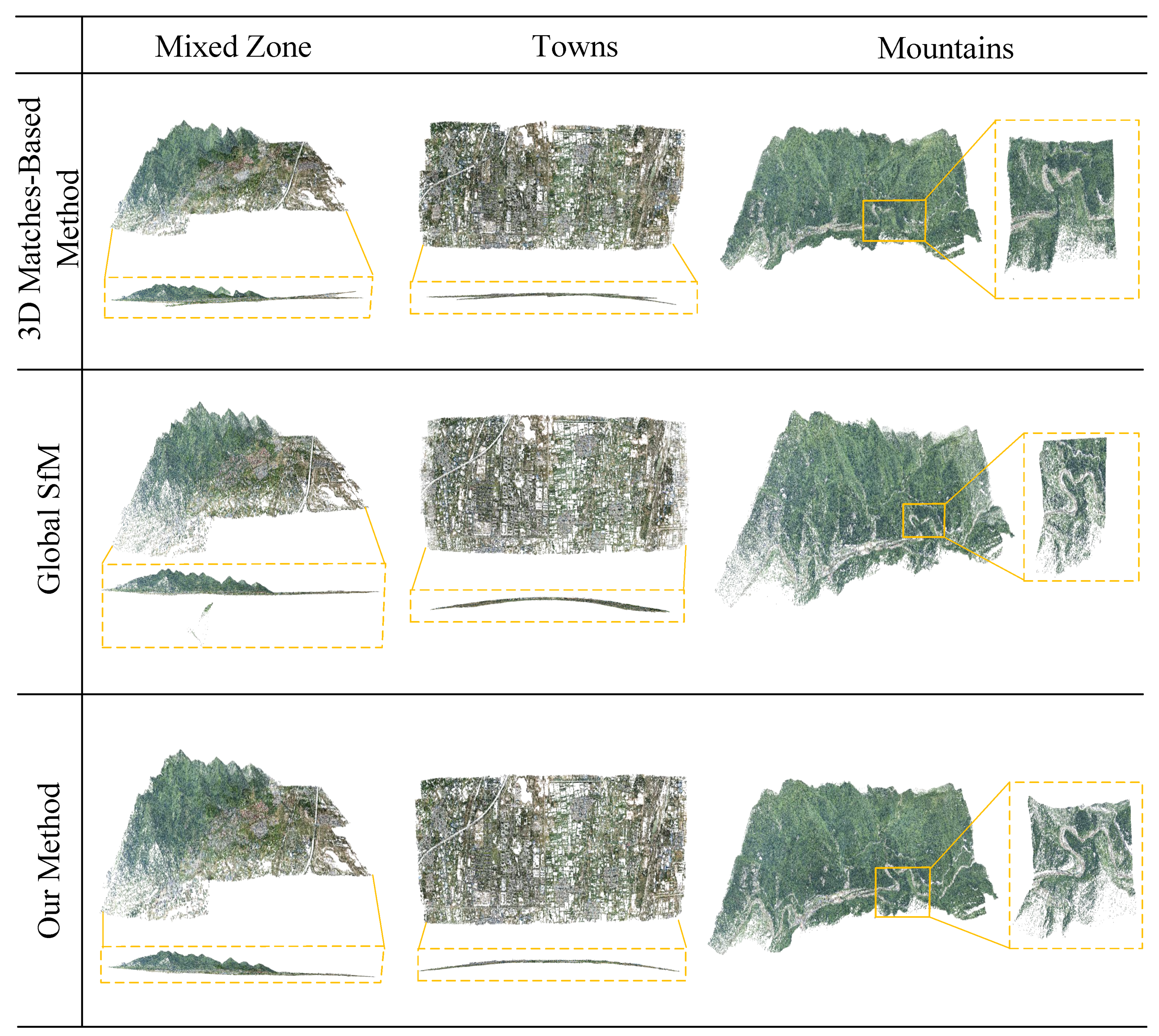
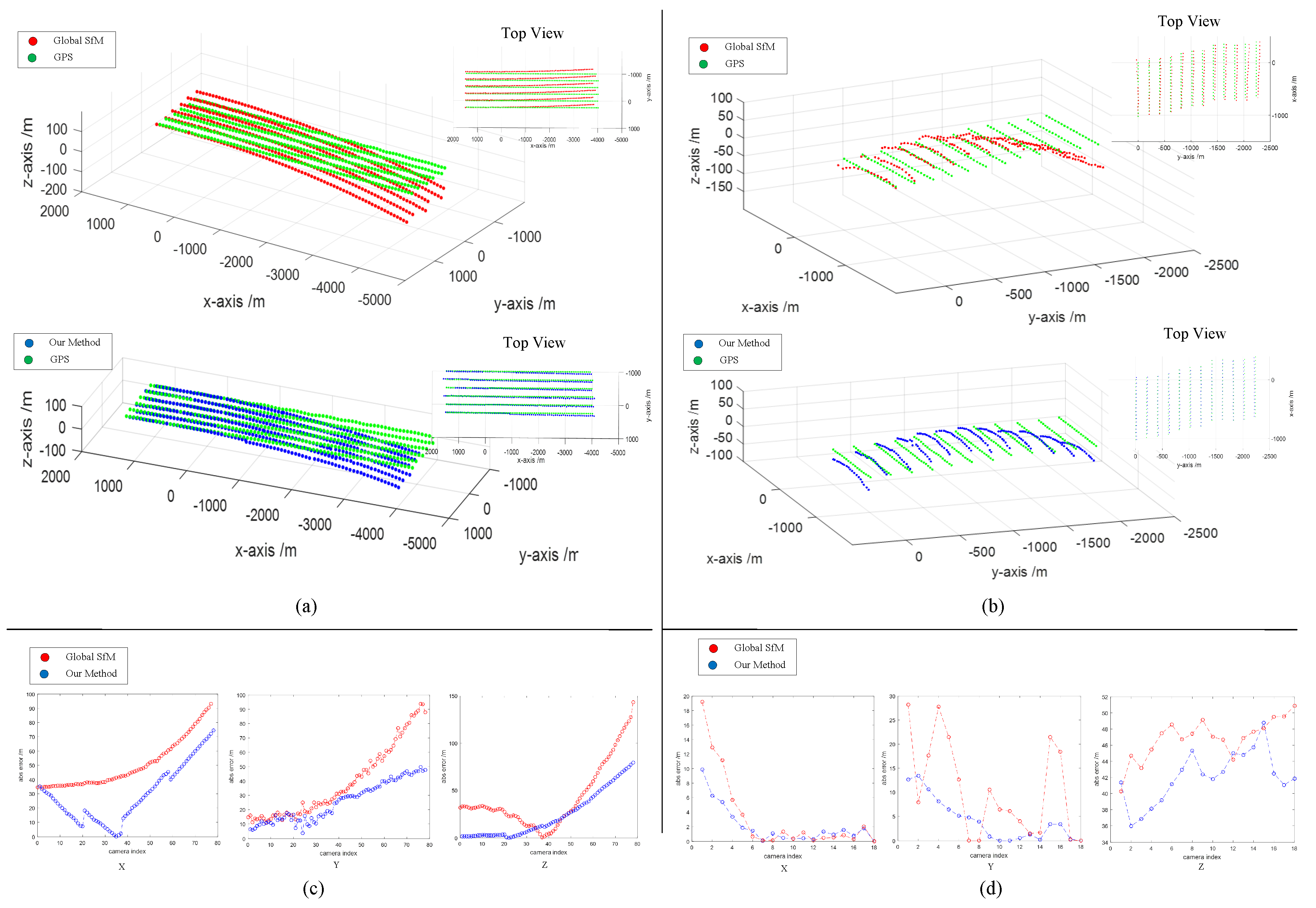
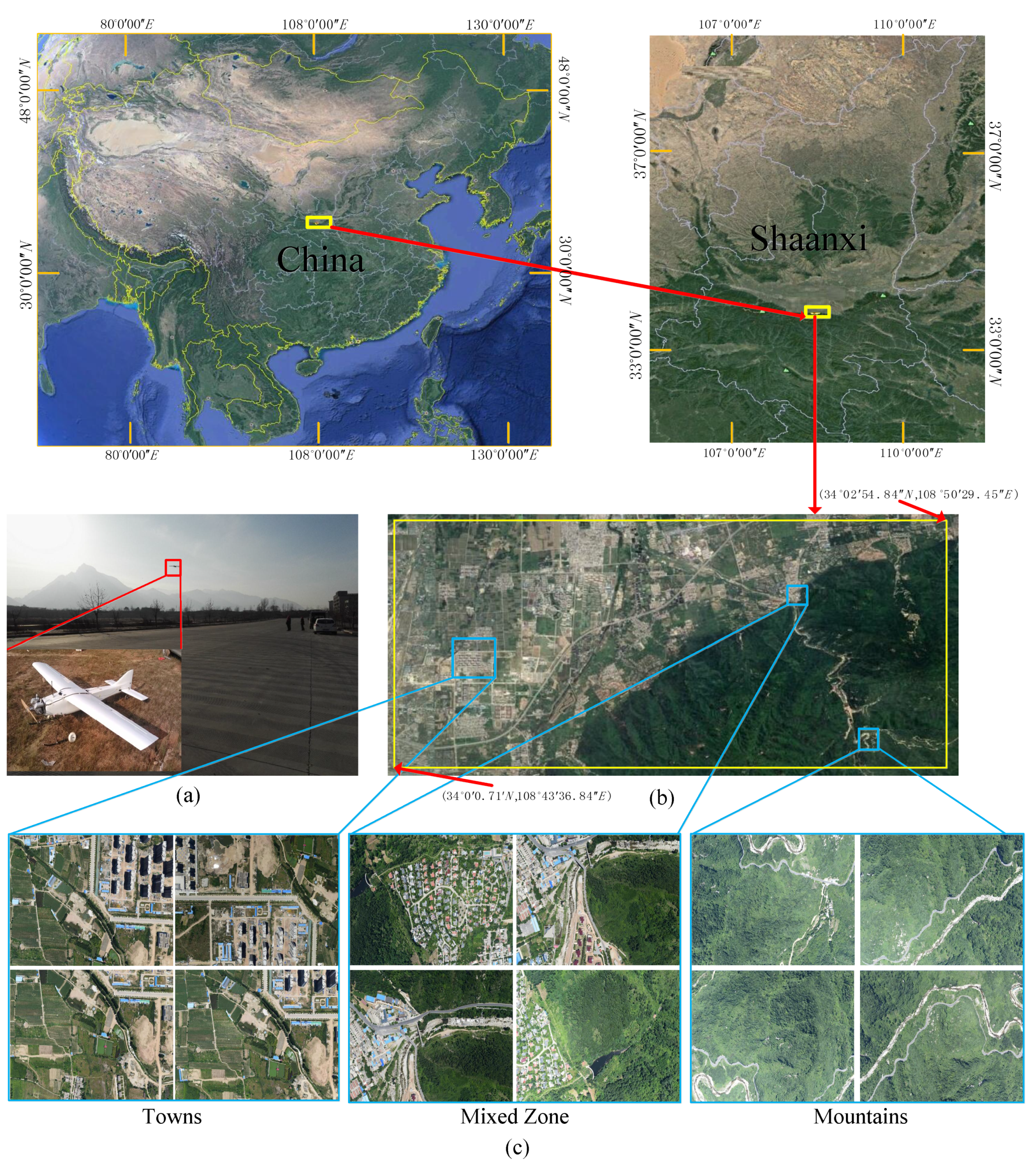
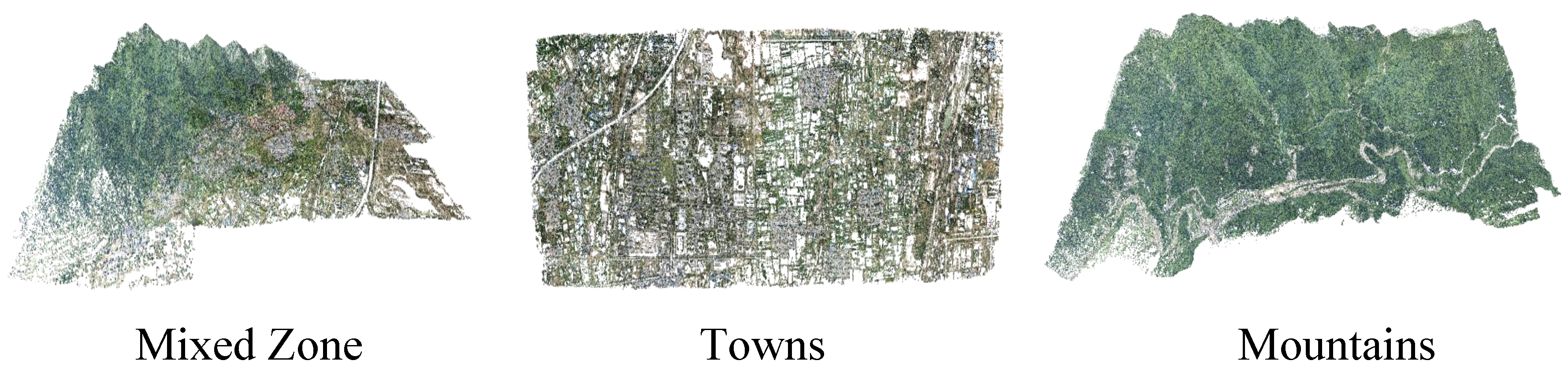
  • Finally, to evaluate the proposed method, we construct a large-scale aerial image dataset named the Qinling dataset, which is captured over Qinling mountain, covering 57 square kilometers. The experiments demonstrate that our method can rapidly and accurately reconstruct a large-scale dataset.
The remainder of the paper is organized as follows. We describe the proposed method in Section 2. Section 3 describes the experimental results. In Section 4, we discuss the proposed method. Finally, we conclude the paper in Section 5.

2. Method

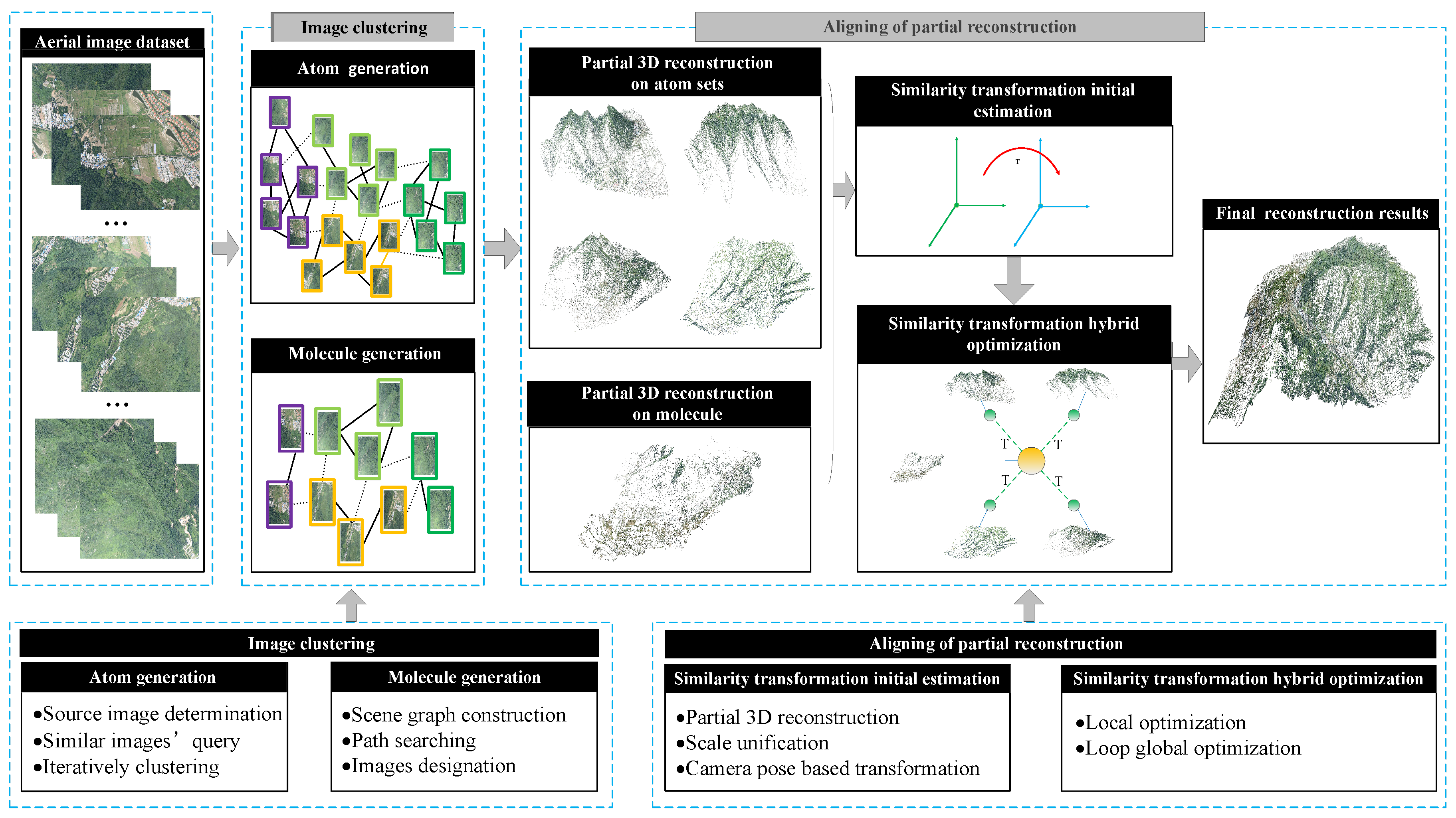
This section elaborates our proposed approach for fast, large-scale 3D reconstruction based on the hierarchical clustering-aligning framework. The flowchart of the proposed method is illustrated in Figure 1.
The framework contains two main parts: image clustering and aligning of partial reconstructions.
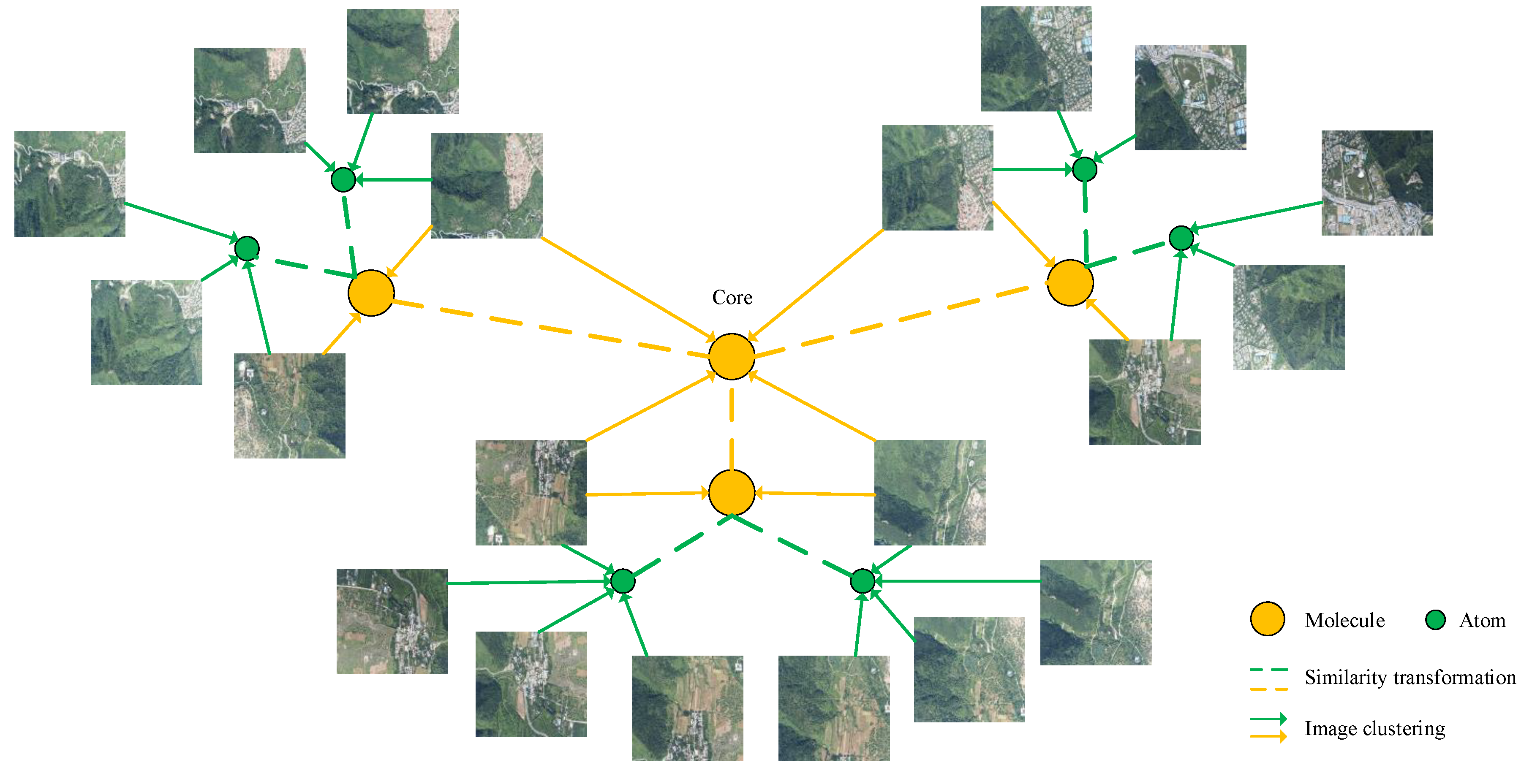
Through image clustering, we obtain the two kinds of associated image subsets. In order to visualize the relationship of the two kinds of image subsets, we use the concept of the hierarchical atomic model, a term used in the chemical field. To distinguish the two kinds of image subsets, we use the concepts of atom and molecule to represent a subset of clustered images, respectively. The hierarchical atomic model is illustrated in Figure 2. The generation of a molecule is related to some adjacent atoms. In fact, the molecule represents an image subset that overlaps with each given image subset represented by atoms. It should be pointed out that the hierarchical atomic model is just a new name for image subset. For large-scale image datasets, the atomic model has two layers, which means the model has multiple molecules and corresponding atoms. For slightly smaller datasets, the atomic model has just one layer, which means the model has just one molecule and corresponding atoms. For large-scale image datasets, multiple groups of adjacent atoms generate multiple molecules. Among these molecules, we determine a core molecule, which overlaps with each other molecule. In this way, we have built a two-layer atomic model in which each atom is associated with the core molecule. This image clustering pattern provides a prerequisite for the follow-up work. For convenience, in the remainder of this paper, we use the atoms and molecules to represent the concept of the image subset. Next, independent partial 3D reconstruction is performed on each atom and molecule. According to the overlapping relationship between each pair of atoms and its corresponding molecules and each pair of molecules, we compute the similarity transformation via joint camera poses of common images across atoms and molecules. Finally, we implement a similarity transformation-based BA hybrid optimization. During optimization, closed-loop constraints between atoms and molecules are applied to correlate pairwise partial reconstructions. With hybrid optimization, we can get the complete seamless scene structure.

2.1. Image Clustering

In this subsection, we perform an image clustering task. The purpose of image clustering is to decompose large-scale SfM into small problems. This has two significant advantages in terms of efficiency. First of all, due to the small number of images in the image subset, the time consumption in the process of feature matching and BA will be significantly reduced, and second, partial reconstruction on the image subset can be performed in parallel.
In addition, the specific image organization pattern caused by image clustering lays the foundation for the subsequent alignment work.

2.1.1. Vocabulary Tree-Based Atom Generation

In the process of the generation of atoms, we use the vocabulary tree [24] to cluster images. The vocabulary tree used in this paper is a standard vocabulary tree with K-branch and L-depth. In the experiment, we use a pre-computed and publicly-available tree [25].
After vocabulary tree establishment, we firstly decide some source images, which are the origins of image clustering. In order to make image clustering more uniform according to the UAV flight path, the source images can be determined from those with long space intervals. Each source image is assigned to an atom. We then iteratively assign similar images to each atom according to the similarity measurement. Considering efficiency, in the image clustering phase, we resize all images to a fixed small resolution; in our experiment, that is 640 × 480. We treat the source images as database images and the remaining images as query images. For each image, Oriented FAST and Rotated BRIEF (ORB) [26] features are detected and converted to weight vectors. Concretely, we define a query vector q for query images and a database vector d for database images according to the assigned weights as:
q i = n i ω i
d i = m i ω i
where n i and m i are the number of descriptor vectors of the query and database image, respectively, with a path through the cluster center node i, ω i is the Inverse Document Frequency (IDF) weight, which is denoted as:
ω i = l n N N i ,
where N is the number of images in the training database and N i is the number of images in the training database containing node i. For each database image, we compute a relevance score with all query images in turn based on the normalized difference between the query and database vector:
s ( q , d ) = q q d d .
N query images with the highest scores are determined by sorting, which means these query images are most similar to the database image. Therefore, we assign these selected query images to the subset with the same label as the database images. Then, we regard these selected query images as new database images and compute the relevance score to search for similar images. We iteratively perform the above process until most images are assigned. Through image clustering, the number of images in each image subset is generally limited to 35–65. The purpose of this is to avoid having too many images in each image subset, which could affect the efficiency of reconstruction, and to avoid fragmented partial reconstruction on each image subset due to having too few images.

2.1.2. Path Searching-Based Molecule Generation

In the process of the generation of molecules, we use graph searching to cluster images. During the image clustering of the atom sets, we detect ORB features from all the resized images. On this basis, we can construct a scene graph. We apply exhaustive feature matching using Fast Approximate Nearest Neighbor (FLANN) [27] to accelerate matching. Then, geometry is verified by computing the geometrical constraint, which can map a sufficient number of features between a pair of images. Based on the pairwise image relations, we can construct the scene graph with the images as nodes and the matching relations of two images as edges.
A molecule is generated by searching for the path in the scene graph between the source images of atoms. During each search for the shortest path, the images on the path are assigned to the molecule. Here, we use the Dijkstra algorithm to search for the shortest path. The significance of searching for the shortest path is that it avoids having an excessive number of images in the molecule. Since the Dijkstra algorithm is applied to the weighted graph, in order to find the shortest path, the edge weight should be set to 1. After counting the paths between any pair of source images, the duplicate images are removed. For the large-scale image dataset, the atomic model has two layers. Concretely, there are multiple molecules in the atomic model. According to the distribution of the source image of each atom in space, we first divide the atoms into multiple groups, and each group of atoms will produce a molecule. According to the distribution of molecules in space, we determine a core molecule. It is necessary not only to count the paths in the scene graph between atoms, but also to count the paths between the source images of the core molecule and each other molecule. We assign all the images involved in these paths to the core molecule. In this way, we have built a two-layer atomic model in which all atoms can be associated with the core molecule.

2.2. Aligning of Partial Reconstruction

After the image clustering task, we make an independent partial 3D reconstruction on each image subset, including the atoms and molecules. In this work, the partial 3D reconstruction is conducted by global SfM [12], including the process from feature detection to the final global BA. To speed up the process, each partial reconstruction could be processed in parallel. It should be pointed out that the images used in partial 3D reconstruction are original images without resizing. The output of partial 3D reconstruction is a sub-model that contains 3D point clouds of the scene structures and camera extrinsic parameters corresponding to images.
In this subsection, we introduce our method to align all partial 3D reconstructions seamlessly. Our method contains two steps: (1) similarity transformation initial estimation and (2) similarity transformation-based BA hybrid optimization.

2.2.1. Similarity Transformation Initial Estimation

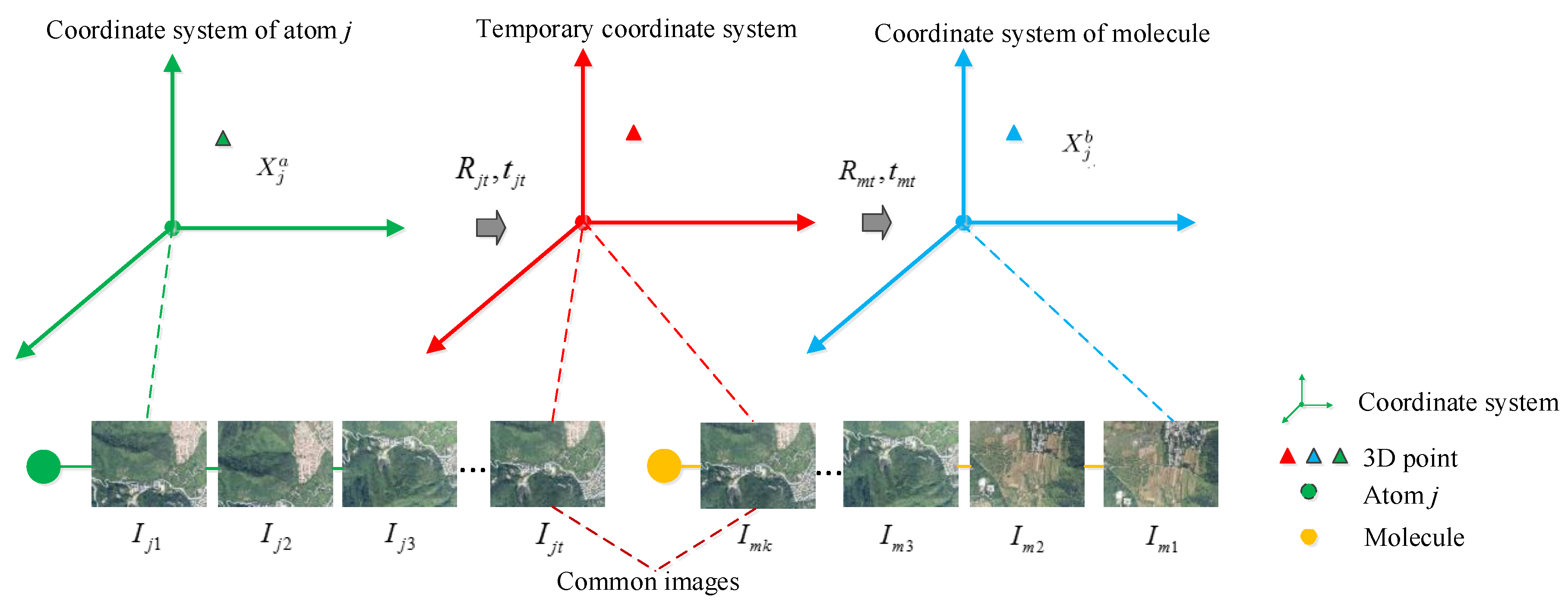
To align a pair of partial reconstructions, a similarity transformation should be computed. Mostly, a similarity transformation between the coordinate systems of the partial reconstructions is computed by means of 3D point matches. However, due to the mismatching on features, the found 3D points do not correspond. In addition, some 3D points may be outliers in the reconstruction process. Therefore, 3D point matching-based similarity transformations are unreliable unless rigorous identification is performed.
In this paper, we propose a concise method to perform a similarity transformation without 3D point matches, as illustrated in Figure 3. Taking a group of atoms and the corresponding molecule as an example, here, we suppose there are L atoms in total. The j th atom shares some common images with the molecule, which are denoted as I j t , , I j k , . Firstly, the scale between the partial reconstructions on an atom and molecule pair should be unified. For each image, we can get its camera center in the frame of the j th atom or molecule. Since the camera model that we used is the basic pinhole model, according to the principle of multiple view geometry [28], supposing an image is I j t , its camera center is defined as:
C j t = R j t T t j t ,
where R j t T and t j t are the transpose of the rotation matrix and the translation vector of image I j t in the frame of the j th atom, respectively. Thus, for any two common images I j t and I j k , the distance of the corresponding camera centers in the frame of the j th atom could be computed as:
d j t k = C j t C j k ,
and similarly, we can get the distance d m t k of the corresponding camera centers for I j t and I j k in the frame of the molecule, which can be represented by:
d m t k = C m t C m k ,
where C m t and C m k are computed with Equation (5) using the rotation matrix and translation vector of images I j t and I j k in the frame of the molecule, respectively. By combining Equation (6) and Equation (7), the scale between the partial reconstructions on a pair of atom and molecule can be computed as:
S = d m t k / d j t k .
After finishing the scale estimation on all pairs of common images between the atom and molecule, the scale is averaged.
Then, we adopt a direct way to get the rotation matrix and translation vector of the similarity transformation by means of the corresponding camera poses of common images shared by atoms and molecules. In other words, we use common images to build a bridge to unify the two coordinate systems. For simplicity, we refer to a common image as a reference view. Without any loss of generality, in practice, we usually select the first common image I j t as the reference view. First, any 3D point X j a of the j th atom should be firstly transformed into the temporary frame of the reference view by means of the rotation matrix R j t and translation vector t j t of common image I j t in the frame of an atom. Then, applying the rotation matrix inverse R m t 1 and translation vector t m t of I j t in the frame of molecule, we get X j b in the frame of molecule, which is represented as:
X j b = R m t 1 [ S ( R j t X j a + t j t ) ] R m t 1 t m t ,
which, when written in matrix form, is:
X j b 1 = T j X j a 1 ,
where T j represents the transformation as:
T j = S R j m t j m 0 T 1
where R j m and t j m are respectively represented as:
R j m = R m t 1 R j t
t j m = R m t 1 ( S t j t t m t ) .

2.2.2. Similarity Transformation Hybrid Optimization

In this part, we elaborate on our optimization strategy. The goal of optimization is to get optimal similarity transformations to make all scene structures of multiple partial reconstructions merge seamlessly. In the initial registration process, we only calculate the similarity transformation based on the camera poses of common images. Therefore, we try to use more 3D points in the optimization process to get a more accurate similarity transformation. In addition, even though we use the 3D points, we still do not need the 3D point matches when optimizing.
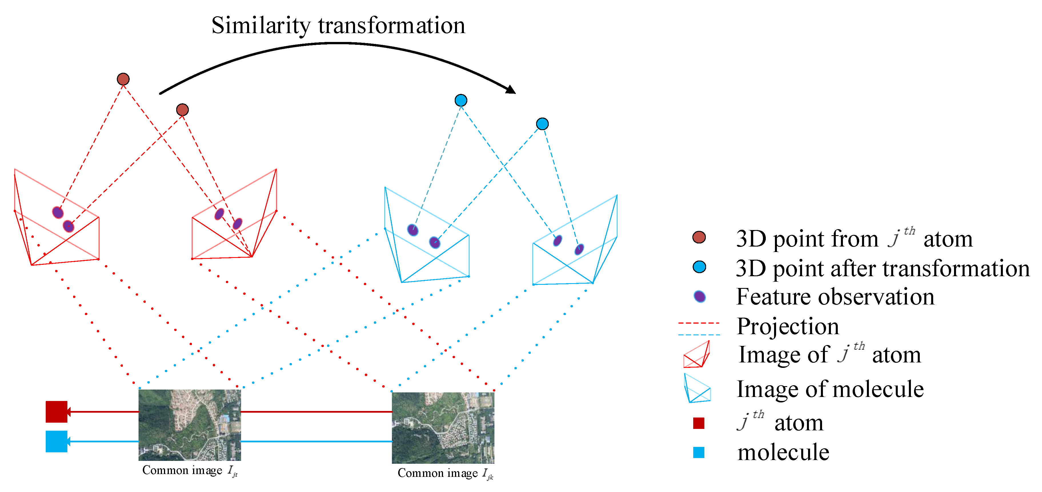
We propose a optimization strategy that is evolved from BA. We firstly introduce a local optimization, which exists between a pair of partial reconstructions, as shown in Figure 4. Without loss of generality, we still use the j th atom and its corresponding molecule as an example. The process of local optimization contains the following steps. In the first step, we get the 3D points reconstructed by common images I j t , , I j k , of the j th atom. From these 3D points, we select some 3D points as data to be optimized, which are observed by at least two common images. By similarity transformation, we can transform these 3D points into the frame of the molecule. In the second step, we perform a BA optimization process in the frame of the molecule. In other words, the transformed 3D points from atom can project into the image planes via the camera poses of common images of the molecule. As the similarity transformation changes, the positions of these transformed 3D points change, and the 2D projected positions change, as well. Therefore, the optimal transformation will minimize the re-projection error. Here, we take advantage of the fact that the features detected from common images of the molecule and atom are consistent. Because the 2D feature observations are the same, the minimum re-projection error means that these transformed 3D points from atoms can replace the original 3D points of the molecule well. Thus, our optimization strategy can be summarized as a BA procedure with similarity transformation, which can be represented as:
min T j j ζ i χ x j i P T j X j i ,
where j is the number of atoms, i is the number of the common 3D points of the j th atom and P is the camera pose of common image I j t in the frame of the molecule. X j i is a common 3D point of the j th atom. In the process of optimization, P is fixed, and X j i is marginalized for efficiency. Through optimization, we can get the optimal similarity transformation between a pair of partial reconstructions.
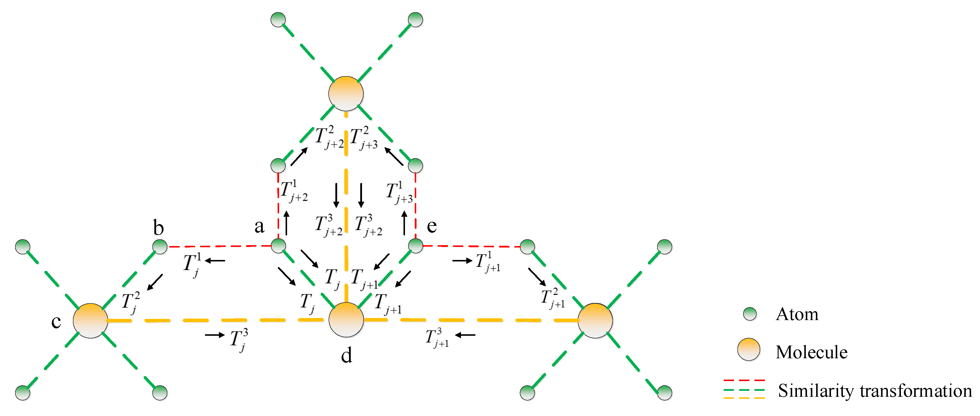
The above optimization process exists in the fusion of a pair of partial reconstructions, including between a pair of molecules and between a pair of an atom and its corresponding molecule. Based on the above local optimization, we propose a loop global optimization strategy. We introduce a closed-loop constraint to incorporate multiple similarity transformations into an optimization process. As we can see from Figure 5, atoms a and b and molecules c and d form a closed-loop through similarity transformations between each pair of them.
Thus, the transformation between atom a and molecule d can be replaced by a continuous transformation of atom a to atom b, atom b to molecule c, and molecule c to molecule d. Therefore, the similarity transformation between atom a and molecule d can be optimized by:
min T j 1 , T j 2 , T j 3 j ζ i χ x j i P T j 1 T j 2 T j 3 X j i ,
where T j 1 , T j 2 , T j 3 represents the similarity transformation between atom a to atom b, atom b to molecule c, and molecule c to molecule d, respectively. Such an optimized process only occurs on adjacent atoms of different atom groups. In order to construct such a closed loop, it is necessary to copy some of the images on the boundary between the adjacent atoms when constructing the atomic model. By combining Equation (14) and Equation (15), we propose a hybrid optimization strategy that can be represented as:
min T j , T j 1 , T j 2 , T j 3 { j ζ i χ x j i P T j X j i + j η i χ x j i P T j 1 T j 2 T j 3 X j i } ,
where ζ represents the index of all pairs of partial reconstructions and η represents the index of closed loops. To solve all of the optimizations defined in Equations (14)–(16), we use the standard Levenberg–Marquardt algorithm [29] implemented in g2o [30] as the solver.

3. Experiments

Extensive experiments were conducted to evaluate the performance of the fast large-scale 3D reconstruction approach based on a hierarchical clustering-aligning framework. We evaluated our method on large-scale aerial image datasets with a high resolution of 7360 × 4912 captured by fixed-wing UAVs. We implemented our algorithm with C++. The experiments in this paper were all performed on an Intel i7 quad core machine with 64 GB RAM. For each image subset, we made an independent partial 3D reconstruction using global SfM [12], implemented in OpenMVG [31], a library for multiple view geometry. Compared to other SfM methods, this algorithm has two major advantages. First, this algorithm has a strong ability to deal with noise. Most global algorithms are actually challenged by noise; however, the reason why this algorithm has better accuracy is that it has a good ability to reject outlier data (wrong point correspondences and false epipolar geometry). This is very important, and it indicates that the algorithm has wide applicability and can be used in a variety of complex environments. Second, this algorithm runs faster, and the rapid completion of partial reconstruction is of great significance for our algorithm framework.

3.1. Datasets

In order to collect a large-scale aerial image dataset, we used high-quality SLR cameras fixed on a fixed-wing UAV (as shown in Figure 6a) to capture images. We used this platform to collect aerial images of about 57 square kilometers of the Qinling mountains (located in Shaanxi Province, China) and surrounding areas through multiple trips. The image dataset is named Qinling. In addition, when capturing each image, we also recorded its Global Positioning System (GPS) value, which could be used as the ground truth for experimental evaluation. These images contained diverse scenarios, such as mountains, towns, and highways. In order to better evaluate the algorithm’s performance in terms of efficiency and accuracy, according to different scenarios, we selected some adjacent local images to form the following image subsets named Mountains, Towns, and Mixed zone, respectively. The image acquisition area and typical aerial images are shown in Figure 6b,c, respectively. Mountains, towns, and mixed zone are subsets of Qinling, each of which also contains hundreds of images. Since our method uses a vocabulary tree and graph searching to cluster images, our algorithm can also be applied to the unordered image dataset. In order to verify the performance of the clustering method on the unordered image dataset, we disrupted the index of the mountains dataset. For large-scale image datasets, in order to reduce the pressure of experimental storage and calculation, we resized the images for the towns and mixed zone image datasets. The statistics of the aerial image datasets are shown in Table 1.

3.2. Experimental Results

First, we evaluated our method on relatively large aerial image datasets, such as mountains, towns, and mixed zone, each of which contains hundreds of images. Thus, in each experiment, after image clustering, we obtained an atomic model with one layer. The number of atoms per image dataset is summarized in Table 1. Then, we made a parallel independent partial 3D reconstruction using global SfM [12] on each molecule and each atom. Finally, the structures from multiple partial 3D reconstructions were merged by means of similarity transformation estimated by our method. The reconstruction results of our method are shown in Figure 7. As we can see, there were no visible vision errors in the reconstructed scene structures.
Finally, we evaluated the proposed method using the Qinling dataset. This is a fairly large dataset of 3849 images, covering a total area of 57 square kilometers. In order to reduce the pressure on experimental storage and calculation, we resized all images to 2560 × 1600. For such a large-scale dataset, in order to avoid having too many images in the molecule after image clustering, we clustered images to get a two-layer hierarchical atomic model. There was a total of 77 atoms and six molecules, where Molecule 2 was determined to be the core molecule. For the molecules, the largest number of images was 120, and for atoms, the largest number of images was 65. Table 2 shows the details of the hierarchical atomic model. Then, we we took the coordinate system of the core molecule as the global coordinate system, Firstly, through the similarity transformation between the atoms and their corresponding molecules, the partial reconstruction results were unified under the molecule coordinate systems, and then through the similarity transformation between the molecules and the core molecule, they were unified into the global coordinate system. Finally, hybrid optimization was applied to make all partial scene structures seamlessly fuse together. The total time of reconstruction from clustering images to getting the final reconstructed scene structure took 112 min 50 s. Figure 8 shows an example of the final reconstruction results. In the top of Figure 8, we show a partial scene structure dynamic merging process of the Qinling dataset, which illustrates the continuity of merging. As we can see from the bottom of Figure 8, the partial scene structures were well aligned. We can see that regardless of the mountain path or the road in towns, the merged scene structure presents a continuous, natural situation.

4. Discussion

4.1. Evaluation Metrics

We used the absolute accuracy of the camera trajectory and the re-projection error of 3D points to evaluate the accuracy of different algorithms, and we used the processing time to evaluate the efficiency of different algorithms.
Here, the re-projection error was obtained by comparing the pixel coordinates (i.e., the observed feature positions) with the 2D positions projected by the 3D points of the partial reconstructions, which were first unified into the global coordinate system by the similarity transformation. The camera trajectory refers to the trajectory formed by the position of the camera as it moves with the UAV. In fact, the reconstructed camera trajectory can be regarded as a series of 3D points, each of which means the position of the camera center. Since we know the GPS of the camera moving with the UAV, after we recover the scale of the reconstructed camera trajectory, we can compare it with the GPS ground truth so as to measure the absolute accuracy of the reconstruction method. The processing time is the total time from loading images to reconstructing the final scene structures. In the experiments of our method, the processing time includes the time for clustering aerial images, the time for parallel partial 3D reconstructions, and the time for calculation and optimization of the similarity transformations.

4.2. Comparison with the 3D Point Matching-Based Method

First, we compared our similarity transformation calculation method with the method based on 3D point matching on the aerial image datasets mountains, towns, and mixed zone. In this comparative experiment, we used standard SIFT [32] for feature detecting and brute-force matching and then filtered out the matches using the fundamental matrix; finally, we calculated the similarity transformation with Random Sample Consensus (RANSAC) [33] using [34] by 3D point matches.
Figure 9 (first row) shows an example of the partial reconstruction fusion results, which were fused by similarity transformation based on 3D point matches. As we can see, the reconstructed structures are not well aligned. Taking the reconstruction result of the towns dataset as an example, from the side view, some partial structures after fusion appear on multiple horizontal planes. In another case of the reconstruction results on the mountains dataset, the mountain road is blocked, since the reconstructed scene structures are not well aligned. Therefore, similarity transformations calculated by 3D matching are not reliable. In contrast, our approach reconstructs the complete scene structures without a visible vision gap (as shown in Figure 9 (third row)). In addition, we show the difference in accuracy between the two methods by re-projection error. Table 3 compares the statistical performances of the two methods. Our method achieves a lower re-projection error. On average, our method only has about 1.0 pixel, far less than the re-projection error of the fusion method based on 3D point matches. As we can see from Table 3, after optimization, the re-projection error will significantly drop before the optimization, which illustrates the significant accuracy improvement brought about by the optimization.

4.3. Comparison with Global SfM

Then, we compared our method with the classic global SfM method [12] on the aerial image dataset. The results of global SfM and our method are shown in the second row and third row in Figure 9, respectively. As we can see, our method has a better visual effect than the global SfM. For example, there are redundant scene structures in the reconstruction results of the global SfM on the mixed zone dataset. From the overall appearance, the scene structures reconstructed by our method appear to be very similar to the results of the global SfM method. In fact, our method usually has a larger number of 3D points. Take the experiments of the towns dataset as an example: global SfM has 446,391 3D points, and our method has 459,362 3D points, which is slightly more than using global SfM. The number of 3D points for each atom is shown in Table 4. The reason that our method could reconstruct more 3D points is that for adjacent atoms, since some adjacent images will observe the same visual content, the partial reconstruction of each of them will have some overlapping scene structures in the adjacent edge regions. Therefore, our method can obtain more reconstruction points. In other words, the integrity of reconstruction of our method could be guaranteed.
However, using global SfM for large-scale scene reconstruction will not only encounter the problem of low efficiency, but also lead to the decline of reconstruction accuracy due to the increase in the number of images. As can be seen from Figure 10a, the model reconstructed by global SfM has an overall curved trend. The cause of this phenomenon is as follows. In essence, global SfM through motion averaging deals with error accumulation effectively. However, with an increase in the number of images, bad feature matching also increases, leading to the increase of errors. In this case, through the motion average, the accuracy of reconstruction decreases, so the reconstructed model shows an overall tendency to bend. However, the scene structure reconstructed by our method also shows a slight bending (as shown in Figure 10b), but this is far less than the bending degree of global SfM. The reason is that the reconstruction result of our method is the fusion of multiple partial scene structures, and due to the small number of images in each group, the bending degree of the model obtained from partial reconstruction is relatively small, so the overall bending degree of the fused model is not as large as that directly reconstructed by the global SfM. Therefore, the accuracy of our method will be better than the global SfM.
To analyze quantitatively the difference in accuracy between our method and the global SfM, we conducted an experimental comparison of the accuracy of the reconstructed camera trajectory. Here, we used the GPS as the ground truth of the camera trajectory. In order to compare the two methods under the same coordinate system, we used the similarity transformation to register the ground truth and the computed coordinate system. Before the registration, a reference point needed to be determined to translate the GPS value into geodetic coordinates. The comparison results are shown in Figure 11a,b. In order to quantitatively show the difference between the reconstructed trajectory and GPS, we computed the absolute difference in the X, Y, and Z axes, respectively. Since the trajectories of the two datasets are both in the shape of periodic bands, for clarity, the shapes of the trajectories can be described as a matrix. Along the UAV moving direction, it is called a row; perpendicular to the UAV moving direction, it is called a column. When calculating the absolute difference between the reconstructed trajectory and the GPS, we summed and averaged the data in the same column. The absolute differences are shown in Figure 11c,d. As we can see, compared to the global SfM, the camera trajectory reconstructed by our method is closer to the ground truth.
On the other hand, our method has a significant advantage in terms of the efficiency. Take the experiment on the mountains dataset as an example: it consumes 19 h 11 min 22 s to get the reconstruction results for the global SfM method. In contrast, it consumes 2 h 12 min 33 s to get the final reconstruction results for our method, specifically including 1 min 30 s to cluster images, 2 h 07 min 20 s for parallel partial reconstruction, and 3 min 43 s for the initial estimation and optimization of the similarity transformation. Thus, it promotes 88.49% in terms of efficiency. Table 5 shows the quantitative comparison results in terms of the processing time on the three aerial image datasets.

5. Conclusions

In this paper, we proposed a hierarchical clustering-aligning framework for fast large-scale 3D reconstruction using aerial images. The framework contains two parts, the image clustering and the aligning of the partial reconstructions. The significance of the image clustering is to decompose the large-scale SfM into a smaller problem and to lay the foundation for the follow-up aligning work. Through image clustering, the overlapping relationship between image subsets is established. Using the overlapping relationship, we initially estimate similarity transformations based on the joint camera poses of common images instead of using 3D matching. Then, we introduce the closed-loop constraint and propose a similarity transformation-based BA hybrid optimization method to optimize the similarity transformations. The advantage of the proposed method is that it can quickly reconstruct scene structures for a large-scale aerial image dataset without compromising the accuracy. Experimental results on large-scale aerial datasets show the advantages of our method in terms of efficiency and accuracy.
In the current work, we used the classic global SfM [12] to make a partial 3D reconstruction on each image subset. In general, global SfM is vulnerable to the challenge of feature mismatching, so global SfM [12] takes a strict filtering of mismatches. When applied to a challenging dataset, once the filtering standard is reached, it will filter some images from the reconstruction set, which contributes to the stability of the reconstruction but introduces the problem that, if the common images between atoms and molecules are all filtered out, our algorithm process will terminate, because our method relies on the partial reconstruction results, including the camera poses and 3D points corresponding to the common images. In future work, a better partial reconstruction method will be adopted. The requirements for the partial reconstruction method are not only precision and efficiency, but also the completeness of the reconstruction. After all, a good partial reconstruction result guarantees the implementation of our method. In addition, in our optimization approach, we used the closed-loop constraint. In fact, there are other constraints that can be used in the atomic model. In future work, we hope to exploit the constraints fully in the atomic model to make the hybrid optimization algorithm more robust.

Author Contributions

X.X. and T.Y. contributed to the idea, designed the algorithm, and wrote the manuscript. Z.L. wrote the source code and revised the entire manuscript. D.L. contributed to the acquisition of the Qinling dataset. Y.Z. provided the most of the suggestions on the experiment and meticulously revised the manuscript.

Funding

This work was supported by the National Natural Science Foundation of China under Grant 61672429, 61272288, and the Science, Technology and Innovation Commission of Shenzhen Municipality under Grant JCYJ20160229172932237.

Acknowledgments

We thank for Qiang Ren for providing supportive comments.

Conflicts of Interest

The authors declare no conflict of interest.

References

  1. Mancini, F.; Dubbini, M.; Gattelli, M.; Stecchi, F.; Fabbri, S.; Gabbianelli, G. Using Unmanned Aerial Vehicles (UAV) for High-Resolution Reconstruction of Topography: The Structure from Motion Approach on Coastal Environments. Remote Sens. 2013, 5, 6880–6898. [Google Scholar] [CrossRef]
  2. Bash, E.A.; Moorman, B.J.; Gunther, A. Detecting Short-Term Surface Melt on an Arctic Glacier Using UAV Surveys. Remote Sens. 2018, 10, 1547. [Google Scholar] [CrossRef]
  3. Yang, T.; Li, J.; Yu, J.; Wang, S.; Zhang, Y. Diverse Scene Stitching from a Large-Scale Aerial Video Dataset. Remote Sens. 2015, 7, 6932–6949. [Google Scholar] [CrossRef]
  4. Sarro, R.; Riquelme, A.; García-Davalillo, J.C.; Mateos, R.M.; Tomás, R.; Pastor, J.L.; Cano, M.; Herrera, G. Rockfall Simulation Based on UAV Photogrammetry Data Obtained during an Emergency Declaration: Application at a Cultural Heritage Site. Remote Sens. 2018, 10, 1923. [Google Scholar] [CrossRef]
  5. Mathews, A.J.; Jensen, J.L.R. Visualizing and Quantifying Vineyard Canopy LAI Using an Unmanned Aerial Vehicle (UAV) Collected High Density Structure from Motion Point Cloud. Remote Sens. 2013, 5, 2164–2183. [Google Scholar] [CrossRef]
  6. Corti Meneses, N.; Brunner, F.; Baier, S.; Geist, J.; Schneider, T. Quantification of Extent, Density, and Status of Aquatic Reed Beds Using Point Clouds Derived from UAV–RGB Imagery. Remote Sens. 2018, 10, 1869. [Google Scholar] [CrossRef]
  7. Jensen, J.L.R.; Mathews, A.J. Assessment of Image-Based Point Cloud Products to Generate a Bare Earth Surface and Estimate Canopy Heights in a Woodland Ecosystem. Remote Sens. 2016, 8, 50. [Google Scholar] [CrossRef]
  8. Schonberger, J.L.; Frahm, J.M. Structure-from-motion revisited. In Proceedings of the IEEE Conference on Computer Vision and Pattern Recognition, Las Vegas, NV, USA, 27–30 June 2016; pp. 4104–4113. [Google Scholar]
  9. Wu, C. Towards linear-time incremental structure from motion. In Proceedings of the IEEE Conference on 3D Vision, Seattle, WA, USA, 29 June–1 July 2013; pp. 127–134. [Google Scholar]
  10. Reich, M.; Yang, M.Y.; Heipke, C. Global robust image rotation from combined weighted averaging. ISPRS J. Photogramm. Remote Sens. 2017, 127, 89–101. [Google Scholar] [CrossRef]
  11. Chatterjee, A.; Govindu, V.M. Robust relative rotation averaging. IEEE Trans. Pattern Anal. Mach. Intell. 2018, 40, 958–972. [Google Scholar] [CrossRef] [PubMed]
  12. Moulon, P.; Monasse, P.; Marlet, R. Global Fusion of Relative Motions for Robust, Accurate and Scalable Structure from Motion. In Proceedings of the IEEE International Conference on Computer Vision, Sydney, Australia, 1–8 December 2013; pp. 3248–3255. [Google Scholar]
  13. Triggs, B.; Mclauchlan, P.F.; Hartley, R.I.; Fitzgibbon, A.W. Bundle Adjustment—A Modern Synthesis. In Proceedings of the International Workshop on Vision Algorithms: Theory and Practice, Corfu, Greece, 21–22 September 1999; pp. 298–372. [Google Scholar]
  14. Steedly, D.; Essa, I.; Dellaert, F. Spectral partitioning for structure from motion. In Proceedings of the IEEE International Conference on Computer Vision, Nice, France, 14–17 October 2003; pp. 996–1003. [Google Scholar]
  15. Ni, K.; Steedly, D.; Dellaert, F. Out-of-Core Bundle Adjustment for Large-Scale 3D Reconstruction. In Proceedings of the IEEE International Conference on Computer Vision, Rio de Janeiro, Brazil, 14–20 October 2007; pp. 1–8. [Google Scholar]
  16. Frahm, J.M.; Fite-Georgel, P.; Gallup, D.; Johnson, T.; Raguram, R.; Wu, C.; Jen, Y.H.; Dunn, E.; Clipp, B.; Lazebnik, S. Building Rome on a cloudless day. In Proceedings of the European Conference on Computer Vision, Heraklion, Crete, Greece, 5–11 September 2010; pp. 368–381. [Google Scholar]
  17. Shah, R.; Deshpande, A.; Narayanan, P.J. Multistage SFM: A Coarse-to-Fine Approach for 3D Reconstruction. arXiv, 2015; arXiv:1512.06235. [Google Scholar]
  18. Farenzena, M.; Fusiello, A.; Gherardi, R. Structure-and-motion pipeline on a hierarchical cluster tree. In Proceedings of the IEEE International Conference on Computer Vision Workshops, Kyoto, Japan, 27 September–4 October 2009; pp. 1489–1496. [Google Scholar]
  19. Toldo, R.; Gherardi, R.; Farenzena, M.; Fusiello, A. Hierarchical structure-and-motion recovery from uncalibrated images. Comput. Vis. Image Underst. 2015, 140, 127–143. [Google Scholar] [CrossRef]
  20. Gherardi, R.; Farenzena, M.; Fusiello, A. Improving the efficiency of hierarchical structure-and-motion. In Proceedings of the IEEE International Conference on Computer Vision and Pattern Recognition, San Francisco, CA, USA, 13–16 June 2010; pp. 1594–1600. [Google Scholar]
  21. Chen, Y.; Chan, A.B.; Lin, Z.; Suzuki, K.; Wang, G. Efficient tree-structured SfM by RANSAC generalized Procrustes analysis. Comput. Vis. Image Underst. 2017, 157, 179–189. [Google Scholar] [CrossRef]
  22. Bhowmick, B.; Patra, S.; Chatterjee, A.; Govindu, V.M.; Banerjee, S. Divide and Conquer: Efficient Large-Scale Structure from Motion Using Graph Partitioning. In Proceedings of the Asian Conference on Computer Vision, Singapore, 1–2 November 2014; pp. 273–287. [Google Scholar]
  23. Sweeney, C.; Fragoso, V.; Höllerer, T.; Turk, M. Large Scale SfM with the Distributed Camera Model. In Proceedings of the IEEE Conference on 3D Vision, Palo Alto, CA, USA, 25–28 October 2016; pp. 230–238. [Google Scholar]
  24. Nister, D.; Stewenius, H. Scalable recognition with a vocabulary tree. In Proceedings of the IEEE International Conference on Computer vision and Pattern Recognition, New York, NY, USA, 17–22 June 2006; pp. 2161–2168. [Google Scholar]
  25. Mur-Artal, R.; Tardós, J.D. Orb-slam2: An open-source slam system for monocular, stereo, and rgb-d cameras. IEEE Trans. Robot. 2017, 33, 1255–1262. [Google Scholar] [CrossRef]
  26. Rublee, E.; Rabaud, V.; Konolige, K.; Bradski, G. ORB: An efficient alternative to SIFT or SURF. In Proceedings of the IEEE International Conference on Computer Vision, Barcelona, Spain, 6–13 November 2011; pp. 2564–2571. [Google Scholar]
  27. Muja, M. Fast approximate nearest neighbors with automatic algorithm configuration. In Proceedings of the International Conference on Computer Vision Theory and Application Vissapp, Lisboa, Portugal, 5–8 February 2009; pp. 331–340. [Google Scholar]
  28. Harltey, R.; Zisserman, A. Multiple View Geometry in Computer Vision; Cambridge University Press: Cambridge, UK, 2003. [Google Scholar]
  29. Nocedal, J.; Wright, S.J. Numerical Optimization, 2nd ed.; Springer: Berlin, Germany, 2006. [Google Scholar]
  30. Kummerle, R.; Grisetti, G.; Strasdat, H.; Konolige, K. G2O: A general framework for graph optimization. In Proceedings of the IEEE International Conference on Robotics and Automation, Shanghai, China, 9–13 May 2011; pp. 3607–3613. [Google Scholar]
  31. Moulon, P.; Monasse, P.; Marlet, R. OpenMVG. Available online: https://github.com/openMVG/openMVG (accessed on 10 October 2018).
  32. Lowe, D.G. Distinctive Image Features from Scale-Invariant Keypoints. Int. J. Comput. Vis. 2004, 60, 91–110. [Google Scholar] [CrossRef]
  33. Fischler, M.A.; Bolles, R.C. Random Sample Consensus: A Paradigm for Model Fitting with Applications to Image Analysis and Automated Cartography. Commun. ACM 1981, 24, 381–395. [Google Scholar] [CrossRef]
  34. Umeyama, S. Least-squares estimation of transformation parameters between two point patterns. IEEE Trans. Pattern Anal. Mach. Intell. 1991, 13, 376–380. [Google Scholar] [CrossRef]
Figure 1. Framework of the proposed method, which contains two main parts: image clustering and the aligning of partial reconstructions. In the first part, we perform image clustering to get two image subsets, named atoms and molecules. Specifically, the images with the same color bounding box belong to the same atom. On the basis of image clustering, we utilize the image repetition relation between atoms and the corresponding molecule to align multiple partial reconstructions. In the aligning process, the similarity transformation is initially estimated by using the joint camera poses of common images and then optimized by our hybrid optimization method to realize a seamless fusion.
Remotesensing 11 00315 g001
Figure 2. An illustration of the hierarchical atomic model. The green circle and yellow circles represent atoms and molecules, respectively. The solid line represents the image clustering process, and the dashed line denotes the similarity transformation between a pair of atoms and its corresponding molecule or pair of molecules.
Remotesensing 11 00315 g002
Figure 3. An illustration of the similarity transformation initial estimation. The estimation of the similarity transformation contains two stages. In the first stage, a transformation can be realized from the frame of the atom to the temporary frame by means of the camera pose corresponding to the common images in the frame of the atom. In the second stage, a transformation from the temporary frame to the frame of molecule can further be realized by means of the camera pose corresponding to the common images in the frame of the molecule.
Remotesensing 11 00315 g003
Figure 4. An illustration of the similarity transformation-based BA local optimization. The optimization process contains two steps. In the first step, 3D points from the frame of the j th atom are first transformed into the frame of the molecule by means of similarity transformation. In the second step, the transformed 3D points are projected into the 2D image plane according to the camera poses of common images in the frame of the molecule. With the change in similarity transformation, the projection positions change as well. When the re-projection error is minimum, the optimal similarity transformation is obtained.
Remotesensing 11 00315 g004
Figure 5. An illustration of the hybrid optimization. A similarity transformation between atom a and molecule d can be represented by T j or by T j 1 T j 2 T j 3 . A closed-loop constraint is formed by a similarity transformation relationship in two directions. The introduction of the closed-loop constraint associates multiple similarity transformations and incorporates them into the global optimization.
Remotesensing 11 00315 g005
Figure 6. (a) UAV platform flying over the Qinling mountains; (b) example of image acquisition area visualized by Google Earth, in which the area surrounded by the yellow bounding box denotes an area of 57 square kilometers. (c) Typical aerial images.
Remotesensing 11 00315 g006
Figure 7. Experimental results of three datasets, from left to right: mixed zone, towns, and mountains.
Remotesensing 11 00315 g007
Figure 8. Example of the partial scene structure dynamic merging process on the Qinling dataset. The gray shaded area represents the reconstructed scene before the next fusion. The purple dotted box denotes the magnification of the fusion details.
Remotesensing 11 00315 g008
Figure 9. Experimental comparison results on three datasets, from left to right: mixed zone, towns, and mountains. From top to bottom, the results of the 3D point matching-based method, the reconstruction results of the global Structure from Motion (SfM) [12], and the reconstruction results of our method. Additionally, the visual differences between the reconstruction results are shown in the rectangular boxes.
Remotesensing 11 00315 g009
Figure 10. (a) The side view of the global SfM [12] reconstruction results on the towns dataset; (b) the side view of our method reconstruction results on the towns dataset.
Remotesensing 11 00315 g010
Figure 11. Experimental comparison results of the accuracy of the reconstructed camera trajectory. (a) and (b) The 3D camera trajectory comparison between the reconstructed camera trajectory and GPS ground truth on the towns dataset and the mountains dataset, respectively. (c) and (d) The absolute value of the difference between the reconstructed camera trajectory and the GPS ground truth on the X, Y, and Z axes in the towns dataset and the mountains dataset, respectively.
Remotesensing 11 00315 g011
Table 1. Details of aerial image datasets and image clustering results of our method.
DatasetSizeImage AmountTotal Number of Atoms
Towns2560 × 16004749
Mountains7360 × 49122166
Mixed Zone2560 × 16004309
Table 2. Details of the hierarchical atomic model on the Qinling dataset.
Molecule IndexTotal Number of AtomsTotal Number of Images for All AtomsTotal Number of 3D Points
1157351,221,873
211435626,680
38412449,574
4219641,028,081
52111111,494,541
Table 3. The re-projection error for experimental comparison results.
DatasetRe-Projection Error
3D Matches Based
Method [32] + [33] + [34]
Our Method
Initial EstimationAfter Optimization
Towns4.783.540.98
Mountains4.721.531.03
Mixed Zone4.273.731.11
Table 4. The statistics of the reconstructed 3D points of our method and the global SfM.
DatasetGlobal SfM [12]Our Method
The Sum of the 3D PointsThe Sum of the 3D PointsThe Number of 3D Points in Each Atom
Index 1Index 2Index 3Index 4Index 5Index 6Index 7Index 8Index 9
Towns446,391459,36264,77635,16842,07465,15764,10234,58239,50655,68158,316
Mountains2,324,6882,410,609428,612370,807456,524513,893395,523245,250
Mixed Zone515,743537,46560,69071,45379,15567,43145,17445,94141,76750,75675,278
Table 5. The processing time for experimental comparison results.
DatasetTotal Time
Global SfM [12]Our Method
Towns33 min 35 s10 min 29 s
Mountains19 h 11 min 22 s2 h 12 min 33 s
Mixed Zone48 min 03 s12 min 10 s

