Article

Combined Lane Mapping Using a Mobile Mapping System

1
School of Remote Sensing and Information Engineering, Wuhan University, Wuhan 430079, China
2
Center for Data Science, Peking University, Beijing 100871, China
*
Author to whom correspondence should be addressed.
Remote Sens. 2019, 11(3), 305; https://doi.org/10.3390/rs11030305
Submission received: 27 December 2018 / Revised: 26 January 2019 / Accepted: 30 January 2019 / Published: 2 February 2019
(This article belongs to the Section Urban Remote Sensing)

Abstract

:
High-definition mapping of 3D lane lines has been widely needed for the highway documentation and intelligent navigation of autonomous systems. A mobile mapping system (MMS) captures both accurate 3D LiDAR point clouds and high-resolution images of lane markings at highway driving speeds, providing an abundant data source for combined lane mapping. This paper aims to map lanes with an MMS. The main contributions of this paper include the following: (1) an intensity correction method was introduced to eliminate the reflectivity inconsistency of road-surface LiDAR points; (2) a self-adaptive thresholding method was developed to extract lane markings from their complicated surroundings; and (3) a LiDAR-guided textural saliency analysis of MMS images was proposed to improve the robustness of lane mapping. The proposed method was tested with a dataset acquired in Wuhan, Hubei, China, which contained straight roads, curved roads, and a roundabout with various pavement markings and a complex roadside environment. The experimental results achieved a recall of 96.4%, a precision of 97.6%, and an F-score of 97.0%, demonstrating that the proposed method has strong mapping ability for various urban roads.

1. Introduction

High-definition mapping of 3D lane lines is widely needed for various tasks [1,2], such as highway documentation, ego-vehicle localization with decimeter- or centimeter-level accuracy [3,4,5,6,7], behavior prediction of vehicles on the road [8,9], and safe route and evacuation plan generation [1,10,11] in autonomous driving systems. Conventional maps only provide street-level information for navigation and GIS systems, while a high-definition map for autonomous driving systems requires the accurate location of every lane. 3D lane lines (lane-level maps) are one of the most important features of high-definition maps. In some GNSS-based studies [12,13,14,15,16], lane-level maps have been generated by driving along the centerline of the road (or lane) with a moving vehicle and then analyzing the GNSS trajectory. Such methods are neither efficient nor accurate because each lane must be driven in multiple times and the path tends to deviate from the real centerline. Therefore, lane mapping requires more efficient and accurate methods.
Some vision-based methods have been proposed to automatically detect and track lane markings from images or videos [17,18,19,20]. However, images and videos are susceptible to shadows cast on the road, natural light and weather conditions [21]. Because images and videos are two-dimensional recordings and lack depth information, photogrammetry-based methods based both on cars [22,23] and unmanned aerial vehicles (UAVs) [24,25] can be used to calculate the 3D coordinates of lane markings through epipolar geometry. However, successful depth measurement depends on texture. Because of the repetitive nature of lane markings, such methods are prone to mismatching and lead to false location. In addition, due to the overlapping of lane markings between consecutive images, the 3D coordinates calculated from different image pairs might be inconsistent for the same lane marking, which results in confusion. Thus, automated lane mapping could be improved by using more robust data sources.
Mobile mapping systems (MMS), equipped with laser scanners, digital cameras, and navigation devices, have been developed since the early 2000s [26,27]. The early MMSs have been used for highway-related application and facility mapping [28]. With the development of GNSS techniques, MMSs have shown great potentials for road inventory mapping, applications related to intelligent transportation systems and high-definition maps [29]. An MMS can simultaneously capture 3D point clouds and images of surrounding objects at highway driving speeds, and record its moving trajectory. After geo-referencing, each 3D point of the lane markings has X, Y, and Z geodetic coordinates that are necessary for 3D lane mapping. Meanwhile, the reflective intensity of the point cloud, which reflects the surface materials of the objects, can be used to distinguish lane markings from the road surface. In addition to point clouds, the road images acquired by the MMS provide a rich texture of lane markings and can be used to improve the robustness of lane marking extraction. Therefore, the MMS provides an abundant data source for lane mapping.
However, the MMS-based lane mapping method also has the following challenges: (1) It is time-consuming to process point clouds because there are millions of noisy, unorganized points. (2) The reflective intensity values of the point cloud measured by the MMS are inconsistent with different scanning ranges, incidence angles, surface properties, etc. (3) Because of the unevenness caused by rutting and the dirt or dust on the road, the intensity of lane markings has considerable interference. (4) Because of the increased range, instrument settings, velocity of the vehicle, and quality of the used MMS, the lane-marking points, especially those far from the vehicle, become very sparse and difficult to recognize. (5) To improve the robustness of lane-marking extraction, taking full advantage of the image texture and reflective intensity of point clouds is necessary.
MMS-based lane mapping methods follow two common steps: road-surface extraction and lane-marking extraction. Many segmentation methods have been proposed to extract the road surface from the large-volume of raw data; these methods can be classified into two categories: planar-surface-based methods and edge-based methods. Planar-surface-based methods adopt model fitting algorithms, such as the Hough transform [30] and RANSAC [31], to directly extract the road surface from the point cloud. However, these algorithms are computationally intensive and time-consuming. Edge-based methods [32,33,34,35,36,37] first detect and fit linear road edges, and then segment the road surface using these edges. Point cloud features, such as the normal vector [32] and elevation difference [33], are commonly used to detect road edges or curbs. To improve the computational efficiency, scan lines [34], grids [35] and voxels [36] are used as the basis of road extraction from the point cloud. Using trajectory data, road edge detection can be sped up by limiting the search along the orthogonal direction of the trajectory [37].
Since lane markings are generally more reflective than the background road surface, the intensity can be used to locate lane markings among the extracted road-surface points. Some studies [31,38,39] used a single global threshold to extract road markings. Smadja et al. [31] implemented a simple thresholding process. Toth et al. [38] selected a global threshold based on the intensity distribution in a search window. Hata and Wolf [39] applied the Otsu thresholding method to find an intensity value that maximized the variance between road markings and road-surface points. However, due to the inconsistency of the reflective intensity, a single global threshold may result in incomplete extraction or false positives. Some studies [40,41,42,43,44] used multithreshold methods to reduce the impact of this inconsistency. Chen et al. [40] selected the peaks of intensity values as candidate lane-marking points for each scan line through an adaptive thresholding process. Moreover, 2D projective feature images generated from 3D points are commonly used to extract road markings [41,42,43,45,46]. Kumar et al. [41] introduced a range-dependent thresholding method to extract road markings from 2D intensity and range images. Using georeferenced intensity images, Guan et al. [42] adopted density-dependent multithreshold segmentation followed by a morphological operation. Soilán et al. [43] selected cells with similar angles in the intensity image as a mask and applied the Otsu thresholding process over each mask. Ishikawa et al. [45] and Hůlková et al. [46] generated 2D images from 3D points to accelerate the calculation. Yu et al. [44] developed a trajectory-based multisegment thresholding method to directly extract road markings from the point cloud. In [44], interference points with similar intensities to road markings were removed by a spatial density filtering method. In contrast to the aforementioned studies, Cheng et al. [47] first performed scan-angle-rank-based intensity correction to directly attenuate the intensity inconsistency and then used the neighbor-counting filtering and region growing processes to remove interference points. For point cloud data, the combination of these two steps could improve the result of road marking extraction. However, the point cloud becomes very sparse and the quality of reflective intensity deteriorates because of the increasing range, the instrument settings, velocity of the car, and the quality of used MMS. In addition, the occlusion of other vehicles results in missing lane-marking points. In such cases, it is difficult to correctly extract lane markings using methods that depend only on point clouds. To meet the need for high-precision lane mapping, the fusion of MMS images and point clouds is necessary.
Preliminary studies on the fusion of MMS images and point clouds have been carried out. Hu et al. [48] and Xiao et al. [49] first estimated the potential road plane using the point cloud and then exploited this knowledge to identify image road features. Premebida et al. [50] generated a dense depth map using the point cloud, and combined the RGB and depth data to detect pedestrian. Schoenberg et al. [51] assigned image pixel grayscale values to the point cloud and then segmented the dense range map. Based on the findings from these studies, the fusion of MMS images and point clouds could make full use of the rich data source acquired by the MMS. To date, however, there are few studies for lane mapping. Thus, this paper aims to introduce a validation method that fuses image texture saliency with the geometrical distinction of the lane-marking point cloud to improve the robustness of lane mapping.
In this paper, a combined lane mapping method using MMS data is proposed. As shown in Figure 1, the proposed method mainly includes the following steps:
  • Road-surface extraction: After the point cloud is gridded, the sudden change in the normal vector is used to locate the curb grids on both sides of the trajectory. Road edges are fitted by the curb grids and used to segment the road points. The inconsistency of the reflective intensity of the road points is corrected to facilitate the subsequent lane extraction.
  • Lane-marking extraction: The 3D road points are mapped into a 2D image. A self-adaptive thresholding method is then developed to extract lane markings from the image.
  • Lane mapping: Lane markings in a local section are clustered and fitted into lane lines. LiDAR-guided textural saliency analysis is proposed to validate the intensity contrast around the lane lines in the MMS images. Global post-processing is finally adopted to complement the missing lane lines caused by local occlusion.
The main contributions of this paper include the following: an intensity correction method was introduced to eliminate the reflectivity inconsistency of road-surface LiDAR points; a self-adaptive thresholding method was developed to extract lane markings from complicated surroundings; and LiDAR-guided textural saliency analysis of the MMS images was proposed to improve the robustness of lane mapping.
The remainder of this paper is structured as follows. Section 2 introduces the proposed methods of lane-marking extraction and lane mapping. The experimental data and results are presented in Section 3, and the key steps are discussed in Section 4. Concluding remarks and future work are given in Section 5.

2. Methods

2.1. Road-Surface Extraction

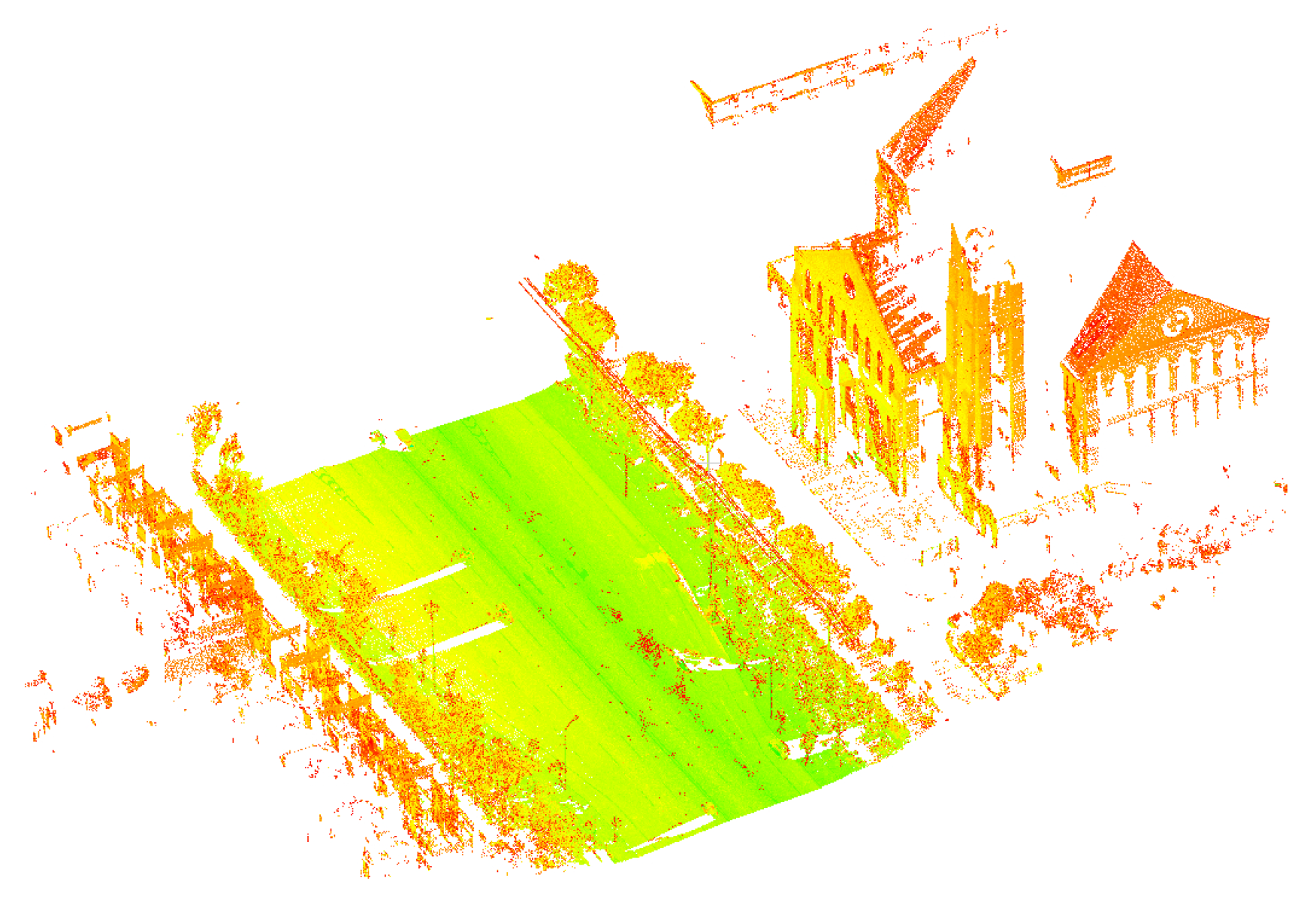
As shown in Figure 2, the point cloud acquired by the MMS contains not only roads, but also buildings, trees, and road facilities such as utility poles. However, lane markings are located only on the road surface and near the vehicle trajectory. In addition, the variation of the elevation of the road surface in a local road section is gentle due to the planar structure of the pavement. To extract lane markings efficiently, this paper roughly delineates the range of the road surface based on the trajectory and elevation statistics, and then removes the points that are outside this range. For the roadside objects in the remaining points, such as flower beds, grasses, and walkways, this paper uses the normal vector to search for the road boundaries and precisely segment the road surface. The reflective intensity of the point cloud is used to distinguish the lane markings from the road background. However, the intensity of the same material in different scanning ranges is inconsistent. To eliminate this inconsistency and obtain the exact intensity contrast between lane-marking and road-surface points, intensity correction is carried out to facilitate the subsequent lane-marking extraction. Therefore, this Section takes the following three steps: (1) Preprocessing: The non-road points are quickly removed. (2) Road extraction: the road surface is extracted by the normal vector. (3) Intensity correction: The intensity of the road points is corrected.

2.1.1. Preprocessing

To quickly remove non-road points, a rough range of the road surface is delineated based on the dense distribution of the pavement points with respect to distance and elevation. Since the road width is limited, the pavement range on the X-Y plane can be determined using the distance from the trajectory. In general, road points in a local road section have similar elevation due to the planar structure. Therefore, the pavement elevation can be obtained based on elevation statistics.
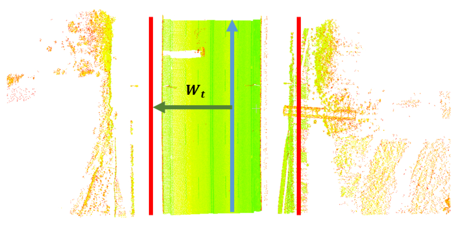
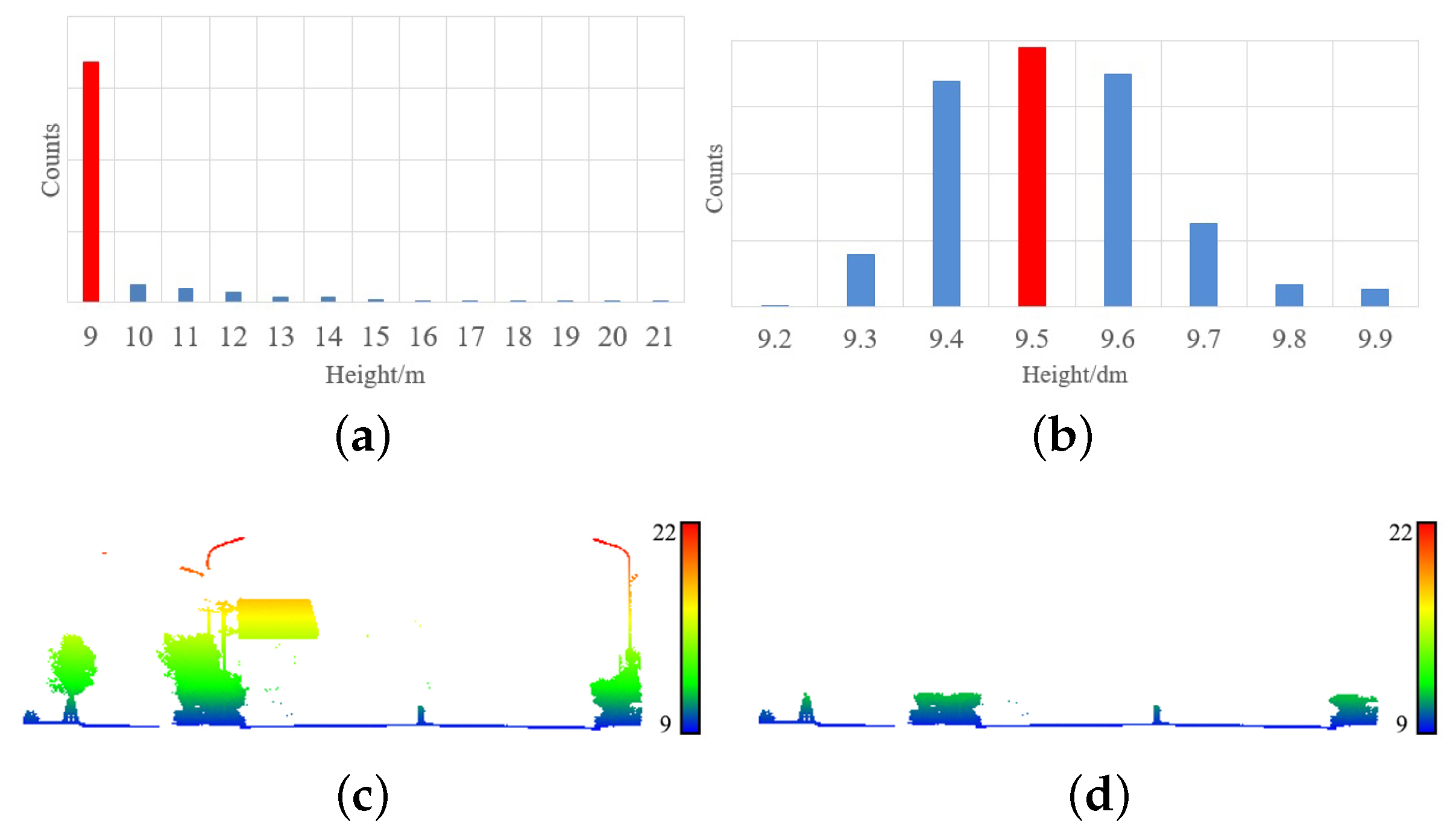
First, the horizontal distance from the point to the trajectory on the X-Y plane is calculated, and points with distance greater than W t are removed, as shown in Figure 3. We set W t = 20 m based on the maximum width of urban roads. Second, the pavement elevation is estimated. Due to the dense distribution and similar elevation of the road points, it is assumed that the elevation histogram of the point cloud in a local road section will show a peak at the pavement elevation. To improve efficiency, a coarse-to-fine statistical method is used. The elevation histogram in meters is first plotted (Figure 4a), and the peak value is set as the coarse pavement elevation. Then, the elevation histogram in decimeters is plotted (Figure 4b), and the fine pavement elevation is obtained. Considering the possible elevation variation of the road slope, points that are 0.5 m below and 1.5 m above the pavement elevation are removed. Figure 4c,d are the point clouds before and after removing non-road points with statistical elevation, respectively.

2.1.2. Road Extraction Based on the Normal Vector

Since an accurate road width cannot be obtained in advance, there are non-road points such as grasses and trees on both sides of the roughly extracted road points. A precise road surface should be extracted to narrow the search range for lane markings. The normal vector of the point cloud is nearly vertical on the road surface, and changes at the road boundaries due to geometric discontinuities, e.g., curbs. Therefore, this paper first locates the curbs using the sudden change in the normal vectors on both sides of the trajectory, and then segments the precise road surface using the road edges fitted from the curbs.
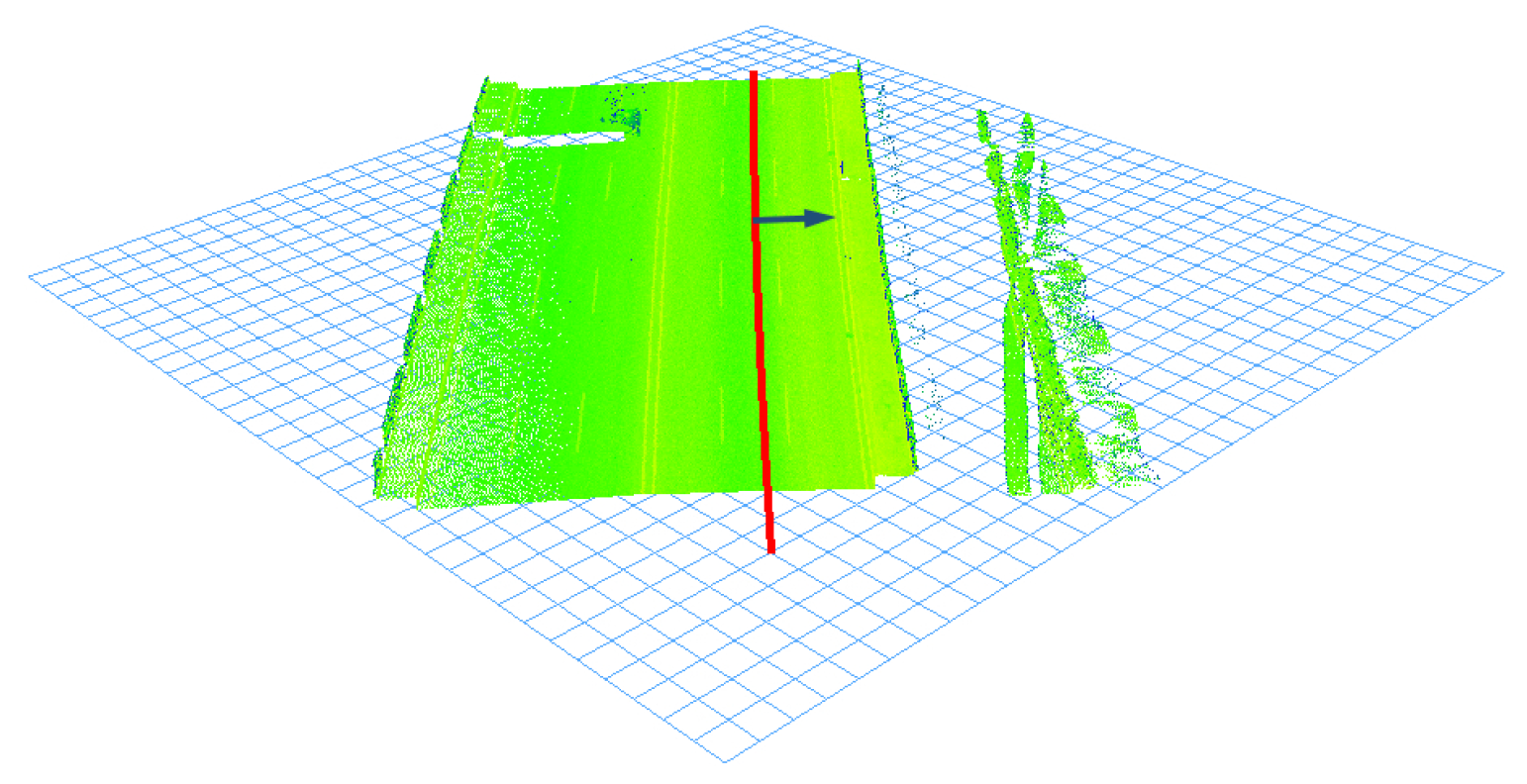
First, the point cloud is organized into regular grids. Then, the bounding box of the point cloud is calculated. With the bounding box, the point cloud is divided into regular grids of a certain length and width, such as 0.5 m, which is equal to the width of road shoulders. The points are then assigned to the corresponding grids based on the X and Y coordinates.
Next, we start from each grid that the trajectory passes through and search for the curb grids along the orthogonal direction of the trajectory, as shown in Figure 5. The PCA algorithm is used to obtain the normal vector of the grid, and the cosine ([0,1]) of the angle between the normal vector and the upright vertical vector is calculated. For each search, the first grid whose cosine is less than A t is considered the curb grid. The threshold A t is set empirically to 0.96 in the experiment.
Finally, the road edges are fitted using the RANSAC algorithm. As shown in Figure 6a, obstacles, such as vehicles on the road, are incorrectly recognized as curbs. The RANSAC algorithm is used to eliminate the false curb grids and fit the inlier ones to road edges. 3D points located between the edges are retained as road points. Meanwhile, the obstacle curbs whose cosine are less than A t are removed. Figure 6b presents the result of road extraction.

2.1.3. Intensity Correction of Road Points

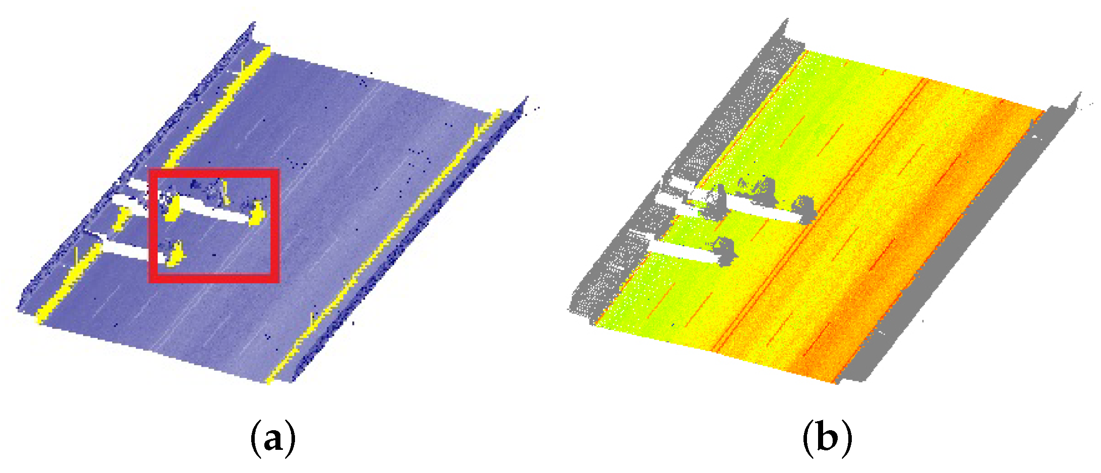
Due to the material difference between lane markings and asphalt or cement pavement, the reflective intensity of road markings is significantly higher than that of the surrounding road points. The intensity can be used to extract road markings. However, in addition to the object material, the intensity measured by the MMS is related to other factors, including the range, incidence angle, sensor characteristics, and atmospheric condition. Since the LiDAR data of a project are measured by the same sensor, the sensor characteristics can be regarded as constant. The atmospheric condition is negligible due to the short range of road points with respect to the vehicle. Moreover, since the height of the scanner is constant during the survey, the cosine of the incidence angle can be described as a function of the range. Therefore, the impact of the range should be eliminated.
Inspired by Kai et al. [52], a correction method is developed to eliminate the range effect by normalizing the original intensity value to a user-defined standard range. A polynomial is established to depict the relationship between range and intensity:
L I = C · i = 0 N ( η i · R i )
where L I is the measured intensity of LiDAR points, R is the range, η i denotes the polynomial coefficients, N is the degree of the polynomial, and C denotes other constant factors. Coefficients η i ( i = 1 , 2 , , N ) are estimated using least square regression using the road points. We set N = 3 in the experiment based on the minimum mean square error. The corrected intensity is shown as follows:
L I R = L I · i = 0 N ( η i · R S ) / i = 0 N ( η i · R i )
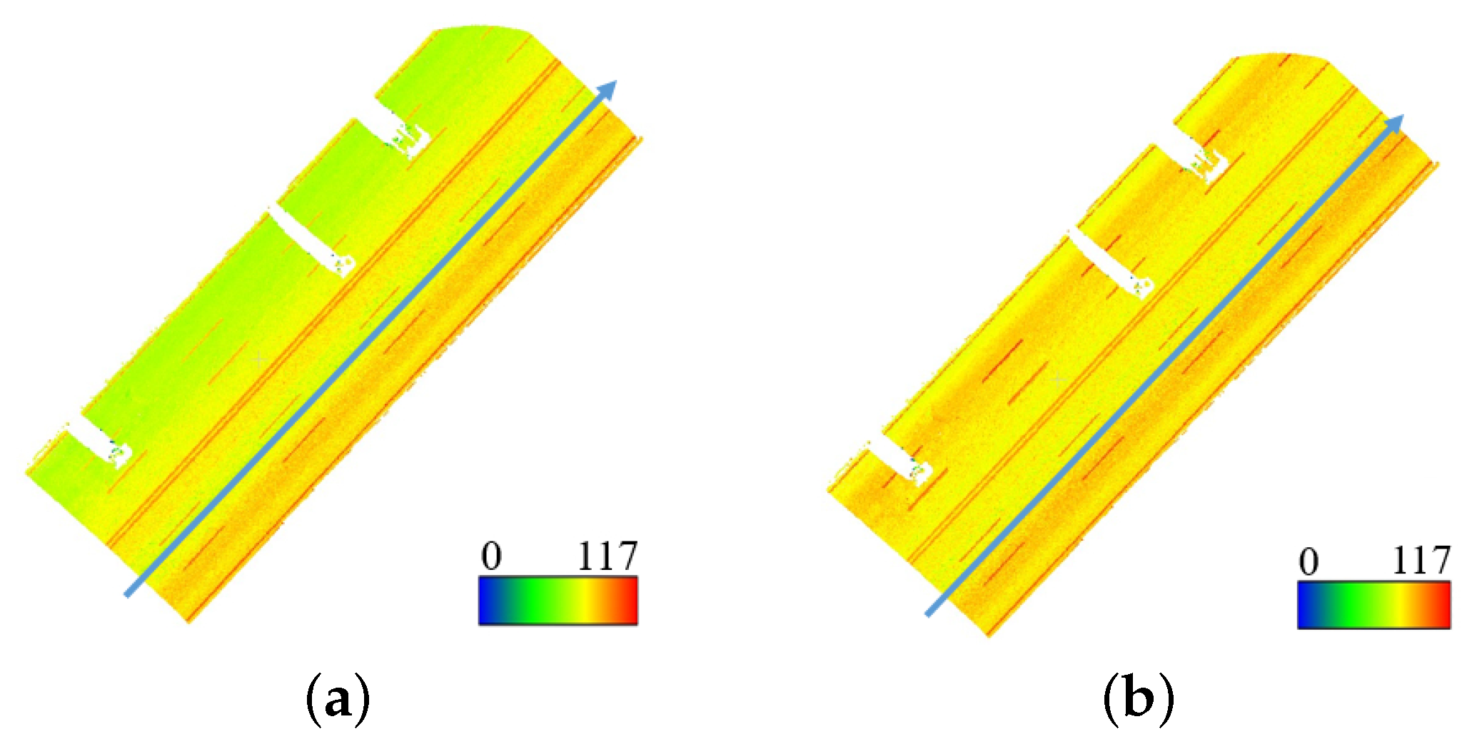
where R S is a user-defined standard range that is set to the average range of the road points. Figure 7a,b are the point clouds before and after intensity correction, respectively.

2.2. Lane-Marking Extraction

Due to the planar feature of the road surface, 3D road points can be mapped to a 2D image. In the 2D image, it is efficient to apply image processing techniques to extract lane markings. Since the elevation information is necessary for the 3D lane map, a correspondence between the 3D point cloud and the 2D image is established and kept. Because of the unevenness caused by rutting and the dirt or dust coverage on the road, lane markings are mixed with noisy and interfering points. As shown in Figure 8, a low threshold value of the reflective intensity leads to considerable noise in (a), while a high threshold value leads to incomplete extraction in (b). Thus, a self-adaptive thresholding method is developed in this paper. First, the large interference region is adaptively located by a median filter, and iteratively suppressed by connected component labeling. Next, the road markings are extracted by maximum entropy thresholding. To remove false positive markings such as zebra crossings, arrows, and stop lines, shape analysis based on the geometric differences is performed. Therefore, this Section takes the following three steps: (1) 3D-2D correspondence: The enhanced road points are mapped into a 2D intensity image. (2) Self-adaptive thresholding: A binary image that contains road markings is generated. (3) Shape analysis: The false negative markings are removed.

2.2.1. 3D-2D Correspondence

Before being mapped to a 2D image, candidate lane-marking points are selected based on the intensity statistics. First, the number of lane-marking candidate points S is estimated based on the laser scanning resolution, the length of the road section, and the width of the lane marking. Then, the road points are sorted by the intensity value in descending order, and points of the top S intensity values are kept as lane-marking candidate points.
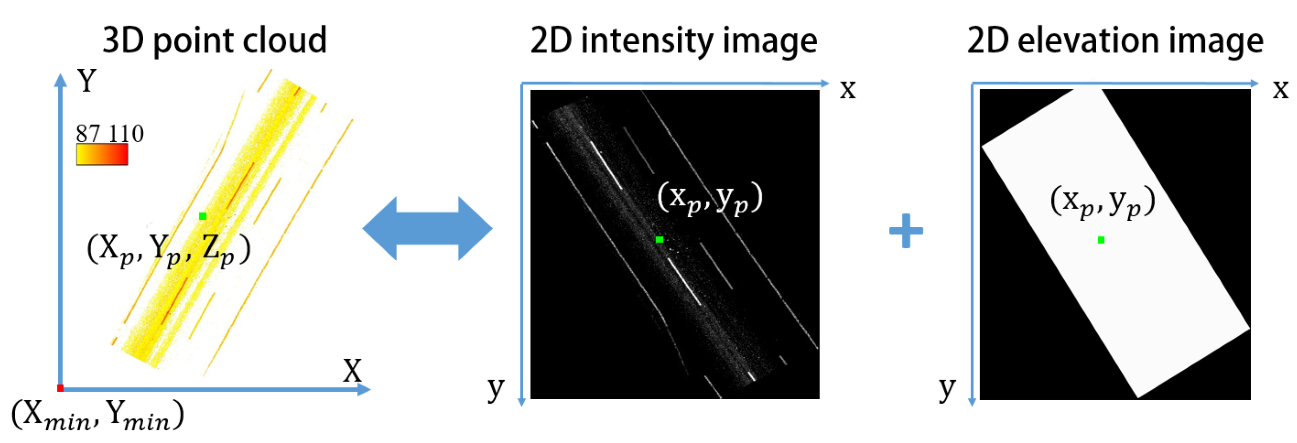
Based on the top view of the candidate points in Figure 9, 2D intensity and elevation images are generated by dividing them horizontally into grids. One pixel of the 2D image corresponds to a grid of top-viewed points. In the experiment, according to the scanning resolution of the points, the length and width of the grids are set to 0.05 m. Since one pixel of the 2D image may correspond to multiple 3D points, the gray value of the 2D intensity image is determined by the average intensity of the 3D points in each grid. To store the elevation information, a 2D elevation image of the same size as the 2D intensity image is generated, and its gray value corresponds with the average elevation. The 3D coordinates of the pixel can be calculated by averaging the 3D coordinates of points in the corresponding grid, as shown in Figure 9. 3 × 3 mean filtering is applied to the 2D images to fill the very small holes caused by the uneven density of the point cloud.

2.2.2. Self-Adaptive Thresholding

For the noisy and interfering points in Figure 10a, a self-adaptive thresholding algorithm is developed. These points are iteratively located and suppressed until there is no large stretch of interference near the lane markings, as shown in Figure 10b. Finally, maximum entropy thresholding is applied to segment the road markings and a binary image is obtained, as shown in Figure 10c.
First, median filtering is used to connect the noisy and interfering pixels in the 2D intensity image. Considering that the width of the lane marking accounts for approximately w l pixels and is much less than that of the interference region, the template size is empirically set to 4 · w l + 1 . Second, maximum entropy thresholding and the connected component labeling algorithm are applied. A connected component with an area larger than the threshold s t is regarded as an interference region. In the experiment, we set s t = 2 · w l · l s e c , where l s e c is the length of the road section. Third, the regional median gray value is subtracted from the interference region. Since the intensity of the road markings is still higher than that of the surroundings, the lane markings in this region are preserved. The above steps are repeated until there is no connected component with an area larger than s t . Finally, maximum entropy thresholding is performed to segment the road markings. Morphological closing is performed to close some very small holes of the segmented lane markings, and connected components that cover less than 0.02 · w l · l l are removed, where l l is the length of the lane marking. Algorithm 1 summarizes the process of self-adaptive thresholding.
Algorithm 1 Self-adaptive thresholding
Require: 
The original image with interference I; The width of the lane marking w l ; The length of the lane marking l l ; The length of the road section l s e c
Ensure: 
The result image, I r e s
1:
r = 4 · w l + 1
2:
s t = 2 · w l · l s e c
3:
a t = 0.02 · w l · l l
4:
repeat
5:
     I b a c k do median filtering to I with r × r template
6:
     I m a s k segment I b a c k with maximum entropy threshold
7:
     { D m a s k i | i = 1 , , n } do 4-connected component labeling to I m a s k
8:
    for i 1 , n do
9:
        if a r e a o f D m a s k i > s t then
10:
            I b a c k ( D m a s k i ) median gray value in I b a c k ( D m a s k i )
11:
        end if
12:
    end for
13:
     I = I - I b a c k
14:
until there exists no D m a s k i that satisfies a r e a o f D m a s k i > s t
15:
I b i n segment I with maximum entropy threshold
16:
I b i n do morphological closing operation to I b i n with a 3 × 3 square structuring element
17:
{ D b i n i | i = 1 , , n } do 4-connected component labeling to I b i n
18:
for i 1 , n do
19:
    if a r e a o f D b i n i < a t then
20:
         I b i n ( D b i n i ) = 0
21:
    end if
22:
end for
23:
return I r e s = I b i n

2.2.3. Shape Analysis: Removal of False Positives

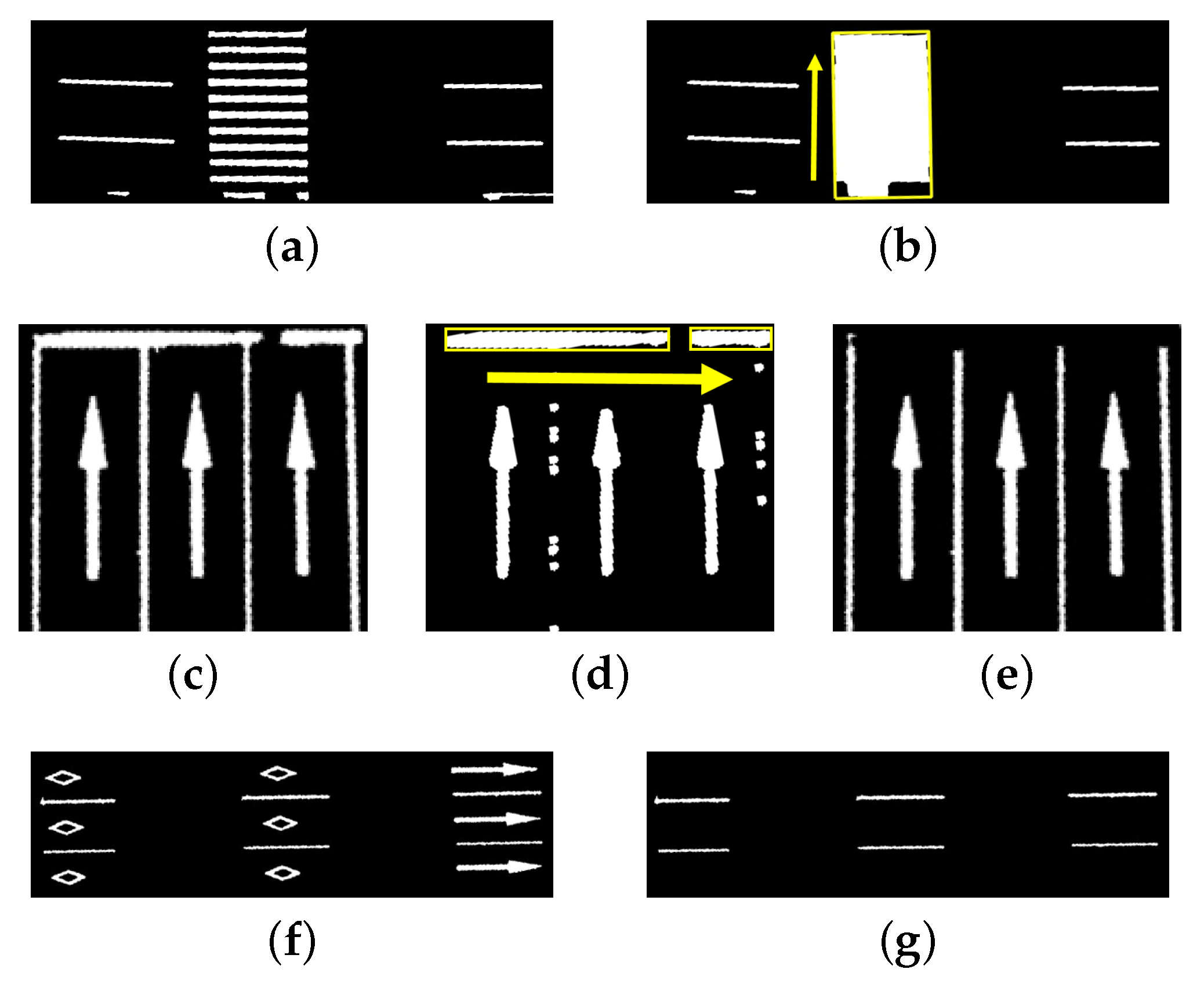
In the binary image, apart from the lane markings, there remain road markings such as stop lines, zebra crossings, arrows, etc. Based on geometric features such as length, width, and orientation, the connected component labeling algorithm and morphological operations are used to remove false positive markings.
  • A single marking of a zebra crossing is similar to a lane marking, but a whole zebra crossing can be distinguished by its crossing orientation, as shown in Figure 11a,b. First, a closing operation is performed over the binary image I b i n to obtain the mask image I m a s k Z C . Next, connected component labeling is performed on I m a s k Z C , and the connected components are denoted D m a s k i ( i = 1 , 2 , , n ) . Finally, the minimum area rectangle of each D m a s k i is calculated and the acute angle θ between the long axis and the trajectory line is obtained. D m a s k i with θ greater than 60 will be regarded as a zebra crossing and removed, i.e., I b i n ( D m a s k i ) = 0 .
  • A stop line is perpendicular to the road but connected to the lane markings, as shown in Figure 11c. Therefore, the stop line can be first separated by an opening operation and then removed by a process similar to the first step, as shown in Figure 11d,e.
  • Road arrows and other road markings, according to the Standards of Road Traffic Marking (2009), have specific lengths and widths. First, connected component labeling is performed on the binary image I b i n , and the connected components are denoted D i ( i = 1 , 2 , , n ) . Second, the length l i and width w i of the minimum area rectangle of each D i are compared with the length l j and the width w j of the standard road markings M j ( j = 1 , 2 , , m ) , respectively. If both conditions of the length and width, i.e., l j - l j × p l l i l i + l i × p l and w j - w j × p w w i w j + w j × p w , where p l and p w are the tolerance of the length and width, respectively, are satisfied, D i is regarded as M j and removed ( I b i n ( D i ) = 0 ) . In the experiment, we set p l = 20 % , p w = 30 % (Figure 11f,g).

2.3. Lane Mapping

To obtain the 3D lane lines of the lane-level map, it is necessary to cluster and refine points belonging to the same lane line, e.g., points of dashed or broken lane markings on the pavement. In a local road section, this paper clusters fragmented lane-marking points based on their deviation from the vehicle’s trajectory and fits them into quadratic curves. Since the point cloud becomes very sparse due to the increase in the range, and the quality of reflective intensity deteriorates at the edge of the road, this paper starts with the near-vehicle lanes and infers lanes near both sides of the road boundary step by step. A LiDAR-guided textural saliency analysis method is developed to validate the intensity contrast around the candidate lines. Finally, a global post-processing step that integrates all local extractions is used to complement missing lines caused by occlusion. Therefore, this Section follows: (1) Local lane line fitting: The local 3D lane lines are fitted from the lane-marking image. (2) Local lane line inference: the candidate lanes near the road boundary are inferred. (3) LiDAR-guided textural saliency analysis: the candidate lanes are projected to the MMS image and validated by textural saliency analysis. (4) Global post-processing: The lane lines are post-processed from global perspective.

2.3.1. Trajectory-Based Local Lane Line Fitting

A lane line in the binary image is not a connected domain due to the dashed or broken lane markings on the pavement. Thus, points belonging to the same lane line should be clustered for lane mapping. In general, the vehicle drives in the same lane, and the deviation between the lane line and the trajectory changes little. Therefore, the deviation is used to cluster the lane-marking points. Considering that the lane line is not necessarily straight, the deviation is calculated along the orthogonal direction of the line segment between two adjacent trajectory points. The steps are as follows.
  • The binary image is first skeletonized to locate the center of the lane markings and reduce the computational burden.
  • The trajectory points (n points) are connected sequentially to form line segments L i ( i = 1 , 2 , , n - 1 ) .
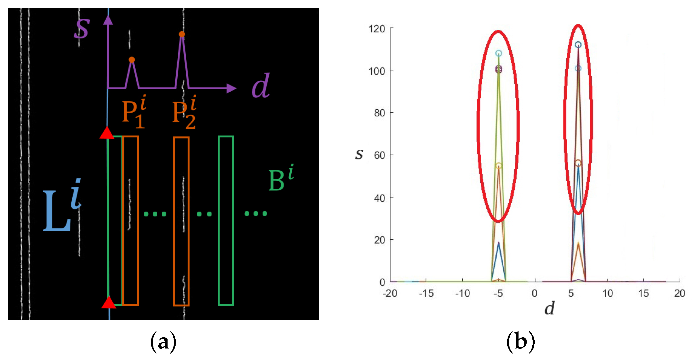
  • As shown in Figure 12a, for each L i , a rectangular buffer B i is generated and moved along the orthogonal direction of L i with a certain step length. The step count and the number of pixels that fall within B i , which are denoted d and s, respectively, are recorded.
  • If the lane-marking pixels fall into B i , s will be larger than the threshold s t and exhibit a peak. The peak buffer is denoted P j i , where j is the number of peaks.
  • For all L i ( i = 1 , 2 , , n - 1 ) , we find P j i ( j = 1 , 2 , ) with its step count d and the pixels that fall within it.
  • The DBSCAN algorithm is used to cluster all peak buffers P j i ( i = 1 , 2 , , n - 1 ; j = 1 , 2 , ) according to their step counts d. The peak buffers of the same lane line will be clustered into a group due to their similar deviation from the trajectory. Figure 12b shows the clustering in an image.
  • The pixels in the peak buffers of a group are fitted by a quadratic polynomial. The 3D points of lane lines are sampled from the polynomial every 0.5 m.

2.3.2. Local Lane Line Inference

The point cloud becomes very sparse with the increase in the range and the quality of reflective intensity deteriorates at the edge of the road. Since several standard values of the lane width are set in the Technical Standard of Highway Engineering (2014), this paper starts with the near-vehicle lane and infers other lanes near both sides of the road boundary step by step until the curb grids are met. Based on the intensity, buffer analysis is performed around the inferred lane lines.
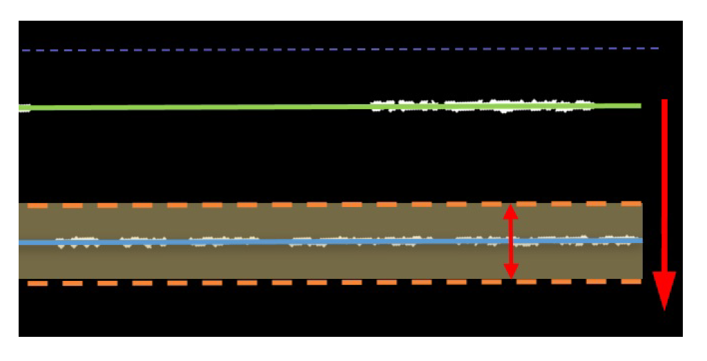
First, the lane width W is determined. The width of the obtained near-vehicle lane (or host lane) is calculated, and W is set to its closet standard value. Next, since the host lane is moved to infer other lanes, the curb grids located in Section 2.1.2 are selected as the boundary to delimit the movement. Finally, buffer analysis, similar to that shown in Section 2.3.1, is used to infer other lanes on both sides step by step until limit W t . As shown in Figure 13, the host lane line is moved parallel to the boundary and white pixels are searched for in a buffer that ranges from W - 0.5 m to W + 0.5 m. If white pixels exist in the buffer, the location where the white pixels match best is selected as a candidate lane line. Otherwise, the host lane line will be moved W in a parallel manner as a default candidate lane.

2.3.3. LiDAR-Guided Textural Saliency Analysis

In addition to point cloud data, the image data acquired by the MMS provides rich texture of lane markings and can be used to further validate the candidate lane lines. The extrinsic parameters between the laser scanner and camera can be obtained by calibrating the MMS. Based on these parameters, a potential region in the MMS image can be determined by mapping the candidate lane line extracted from the point cloud onto the MMS image. Since the lane marking is salient and linear compared with its surroundings, textural saliency analysis is applied to validate the intensity contrast in the potential region.
First, the 3D candidate lane points are mapped onto the MMS image plane. Figure 14a illustrates the relationship between the geodetic, inertial measurement unit (IMU) and camera coordinate systems. The geodetic coordinates of the 3D point [ X W , Y W , Z W ] T should be mapped into the IMU coordinate system first using the geodetic coordinates of the IMU origin C I W and the rotation matrix R I W calculated by the attitude information (e.g., roll, pitch, and heading). Then, based on the collinearity equation, the camera coordinates [ x , y , - f ] T of the mapped pixel can be calculated using the translation C C I and the rotation matrix R C I from the IMU origin to the camera origin, which are obtained by calibration. The formula is as follows:
x y - f = ( R W I · R I C ) - 1 X W Y W Z W - C I W + R I W · C C I
As Figure 14b shows, the column u and row v of the mapped pixel can be calculated by the following formulas:
u = x
v = i m g H e i g h t - y
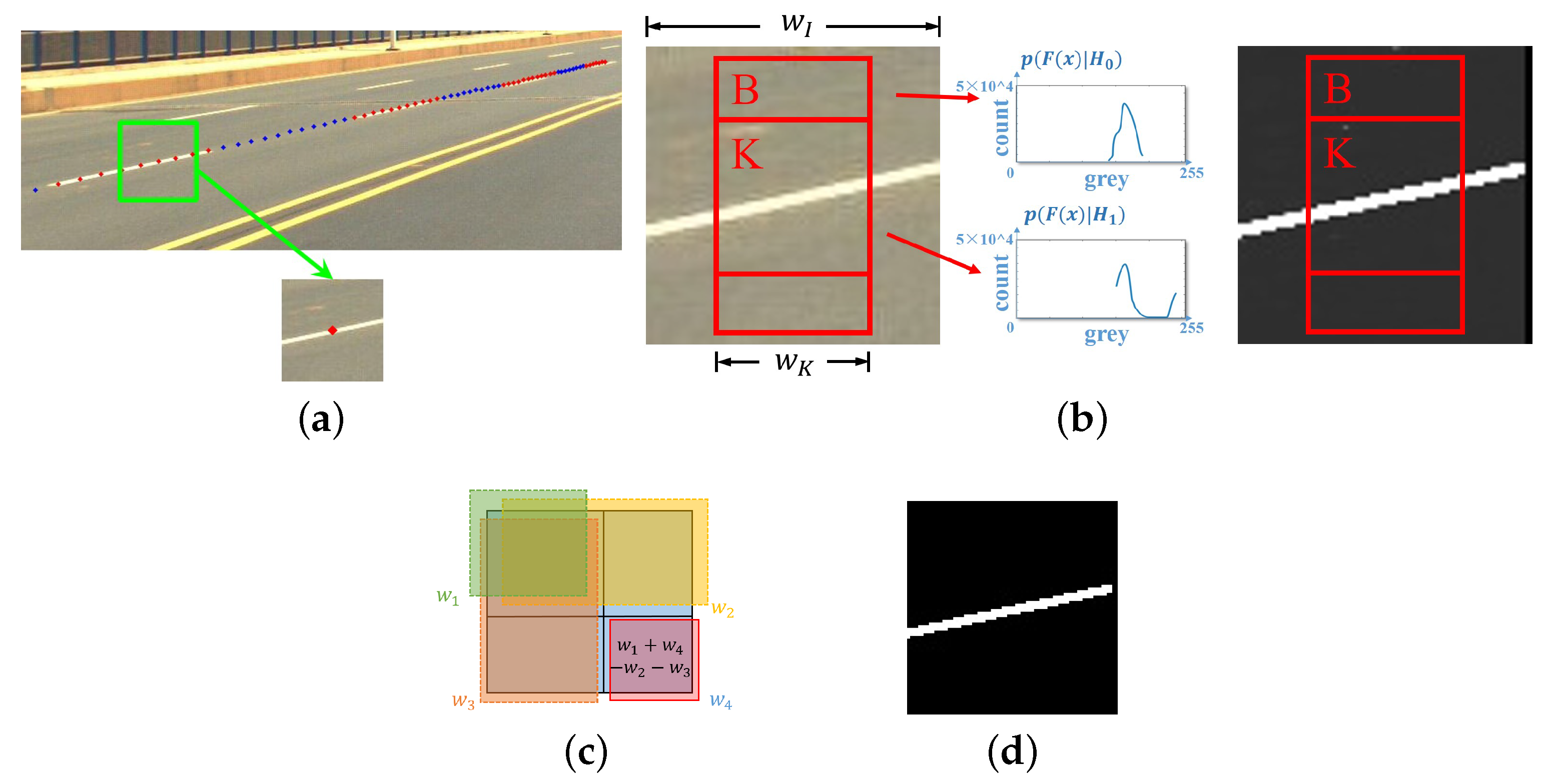
Considering that the width of the lane markings is approximately 0.2 m, a 1 m wide buffer around the candidate lane line points is enough for guiding the textural analysis in the image. As shown in Figure 15, because of the grayscale difference, the lane markings are the most salient in the buffer. Therefore, the existence of lane markings can be validated by textural saliency analysis. From the perspective of posterior probability, an integral histogram algorithm is used to contrast the distribution of the objects and surroundings and estimate the saliency of the pixels [53].
The candidate lane line is sampled at intervals of 0.5 m, and a group of square buffers are obtained by mapping the 1 m wide area around each sampling point to the image, as shown in Figure 16a. In each buffer, a kernel window K containing the lane marking and a border window B containing its surroundings are used to estimate the saliency of the sampling points, as shown in Figure 16b. The gray value of a pixel x in the buffer is denoted F ( x ) . Two hypotheses are defined, i.e., H 0 : x is not salient, and H 1 : x is salient. The corresponding a priori probabilities are denoted P ( H 0 ) and P ( H 1 ) , respectively. The saliency of x can be measured by the posterior probability P ( H 1 | F ( x ) ) . Based on Bayes’ theorem, we can define
P ( H 1 | F ( x ) ) = p ( F ( x ) | H 1 ) P ( H 1 ) p ( F ( x ) | H 0 ) P ( H 0 ) + p ( F ( x ) | H 1 ) P ( H 1 )
where p ( F ( x ) | H 1 ) and p ( F ( x ) | H 0 ) are the distribution of gray values in windows K and B, respectively, as shown in Figure 16b. The saliency measure reflects the contrast of the gray values between windows K and B. The width of the buffer is denoted w I , and we set the width of the kernel window w k = 0.3 · w I to cover the lane marking. Due to the slope of the lane markings in the image, the border window B is obtained by expanding the top and bottom of the window K by 25%. Since lane marking occupies a small area in the buffer, we set P ( H 1 ) = 0.2 and ( H 0 ) = 0.8 . The window slides within the buffer to make sure that all lane-marking pixels are detected. An integral histogram is used to quickly calculate the grayscale histogram in each slide window, as shown in Figure 16c.
The saliency values in the buffer are then segmented by the threshold S t , as shown in Figure 16d. We set S t = 0.8 in the experiment. If a linear object exists in Figure 16d, the corresponding sampling point is considered valid. For each candidate lane line, we denote the number of all sampling points as n and the number of valid points as m. Considering the dashed lane markings and occlusion, the candidate lane line is considered valid if m / n 50 % . An example is given in Figure 16a.

2.3.4. Global Post-Processing

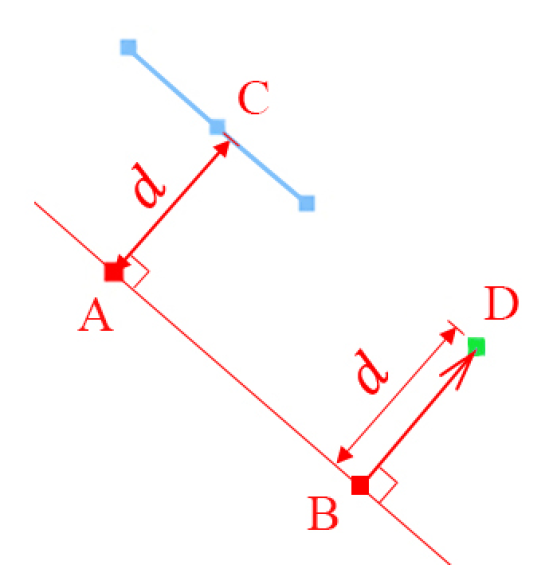
After local lane mapping, 3D points of lane markings are sampled and validated. There are some missing lane line points due to occlusion. This paper uses the global continuity of the lane lines to complement the missing points. If the distance between two adjacent lane line points is greater than the threshold D t h r e , we move the corresponding trajectory points to complement the missing points as illustrated in Figure 17. Finally, B-spline curve fitting is used to smooth the lane-level map.

3. Results

3.1. Experimental Data

The data in this paper were collected using a real-time 3D LiDAR scanner Velodyne HDL3 with 700,000 measurements per second, a horizontal field of view of 360 and a typical accuracy of ±2 cm. The reflective intensity can be simultaneously measured. The navigation system integrates a GNSS satellite positioning module and an IMU. The images are obtained by a Point Grey camera with a resolution of 2448 × 2048. Therefore, the 3D point clouds, images, and trajectory data that we need in this paper can be simultaneously obtained while the vehicle moves.
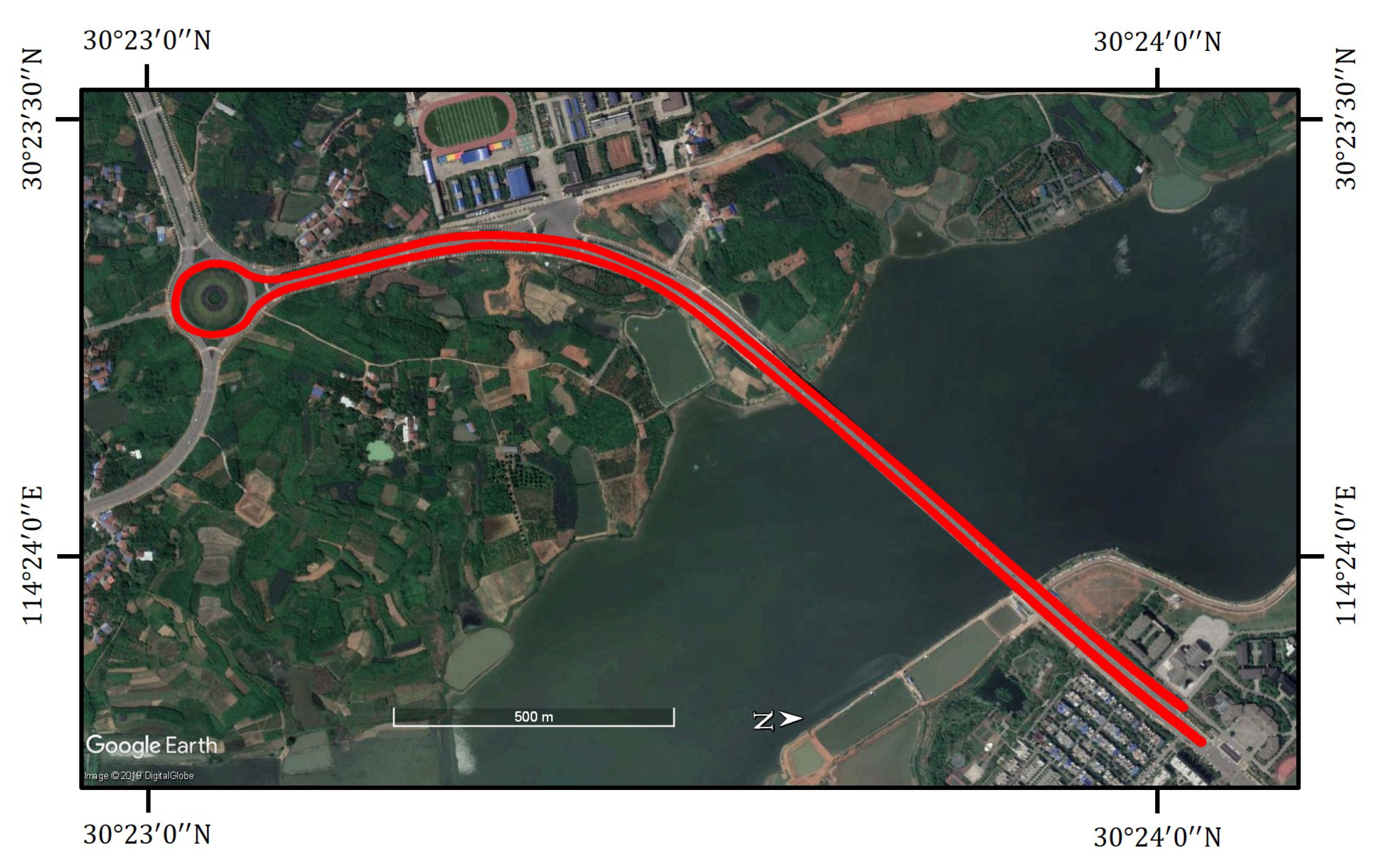
The collected data are located around a bridge in Jiangxia District, in the city of Wuhan, Hubei, China. As shown in Figure 18, the data cover approximately 3.6 km of a two-way six-lane road and a roundabout with four-lane entrances. The two-way road is separated by the double yellow line or guardrail around the center and has straight and curved parts. There are diverse objects (e.g., flower beds, grasses, walkways, etc.) on the roadside and vehicles on the road. In addition, there are various road markings on the road, such as zebra crossings, stop lines, arrows, and diamond markings. Due to unevenness caused by rutting and the dirt or dust covering the road surface, the lane markings are subject to noise and interference. Moreover, the point cloud is very sparse toward the roadside, and the quality of reflective intensity deteriorates near the road boundaries.

3.2. Evaluation Method

The resulting lane-level map is compared with the ground truth that is the centerline of the lane markings and manually annotated by professional operators. The result is considered true if it falls within a 10-cm-wide buffer of the ground truth. The evaluation criteria are given as follows:
P r e c i s i o n = T P T P + F P
R e c a l l = T P T P + F N
F s c o r e = 2 · P r e c i s i o n · R e c a l l P r e c i s i o n + R e c a l l
where T P , F P , and F N are the lengths of the true positive, false positive, and the false negative lane lines, respectively. It is clear that higher precision means fewer false positives and higher recall means fewer false negatives.

3.3. Experimental Results and Evaluation

3.3.1. Typical Cases

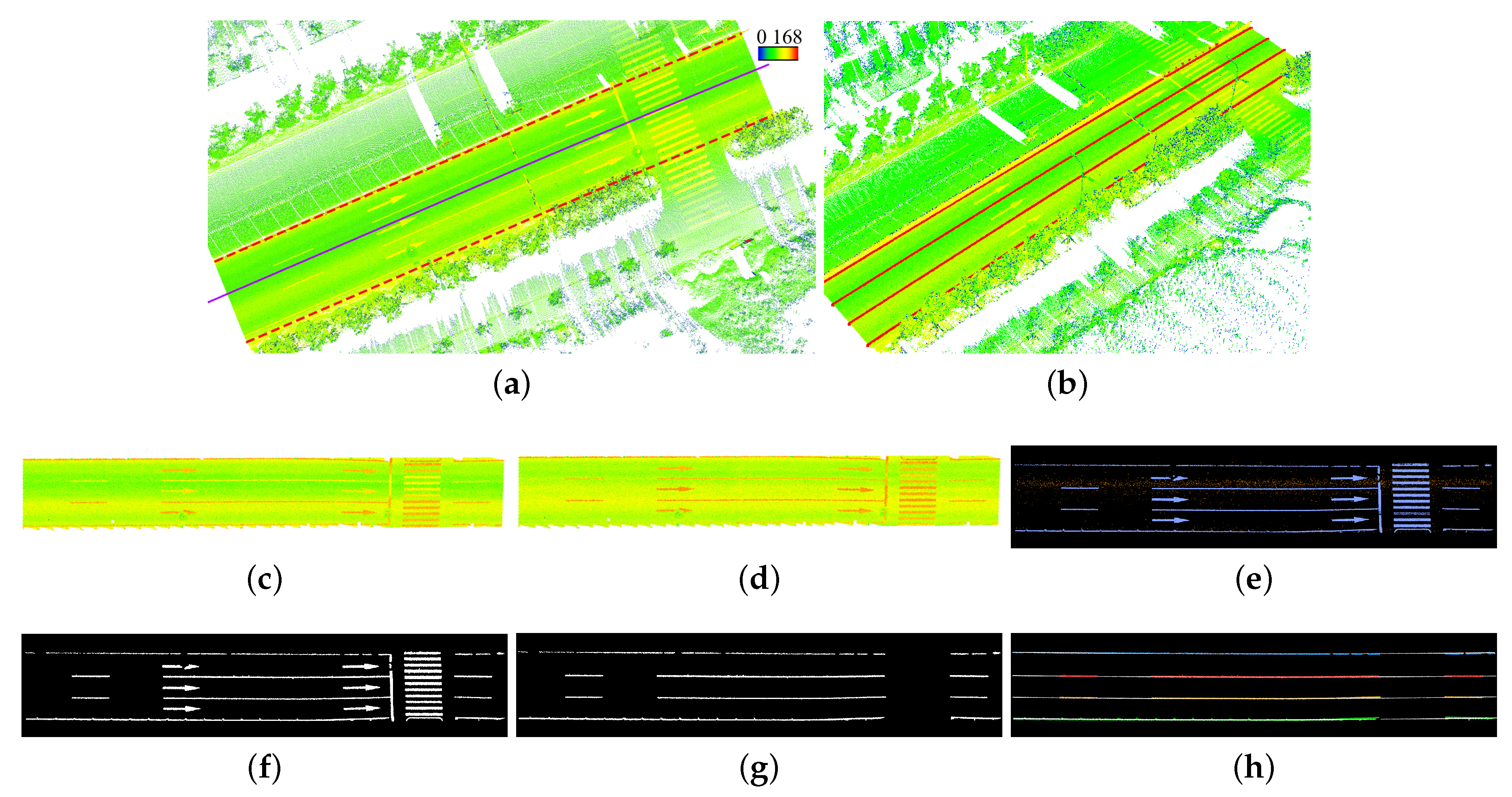
As shown in Figure 19, a typical road section is selected to illustrate the process of local lane mapping using the proposed method. The raw point cloud (Figure 19a) is a three-lane road that is separated by the guardrail and the roadside hedge, with six straight arrows, a stop line, and a zebra crossing on its surface. First, as shown in Figure 19a, starting from the trajectory (the solid purple line), the curb grids that contain the guardrail and roadside hedge are located and fitted into two edges (the dotted red line). The road points (Figure 19c) are segmented by these edges. The number of points is reduced to 40% of the raw data, which reduces the computational burden. Then, intensity correction is performed to eliminate the inconsistency caused by the range. As presented in Figure 19d, the intensity of the points at the left of the trajectory (the upper points) is significantly enhanced. Based on the laser scanning resolution, the length of the road section and the width of the lane markings, 8% of the points with higher intensity are further selected to speed up the extraction of lane markings. A 2D intensity image (Figure 19e) is generated by horizontally mapping these 3D points into regular grids, with interference (the orange part) distributed along a lane. Through self-adaptive thresholding, the interference region is iteratively located and suppressed, and a binary image that contains road markings is generated (Figure 19f). After false positive markings (e.g., straight arrows, a zebra crossing, a stop line) are removed by shape analysis, a binary image (Figure 19g) that contains only the lane markings is obtained. Finally, the lane-marking pixels are clustered based on their deviation from the trajectory, and fitted into lane lines in this road section (Figure 19h). The 3D lane lines are presented in Figure 19b.
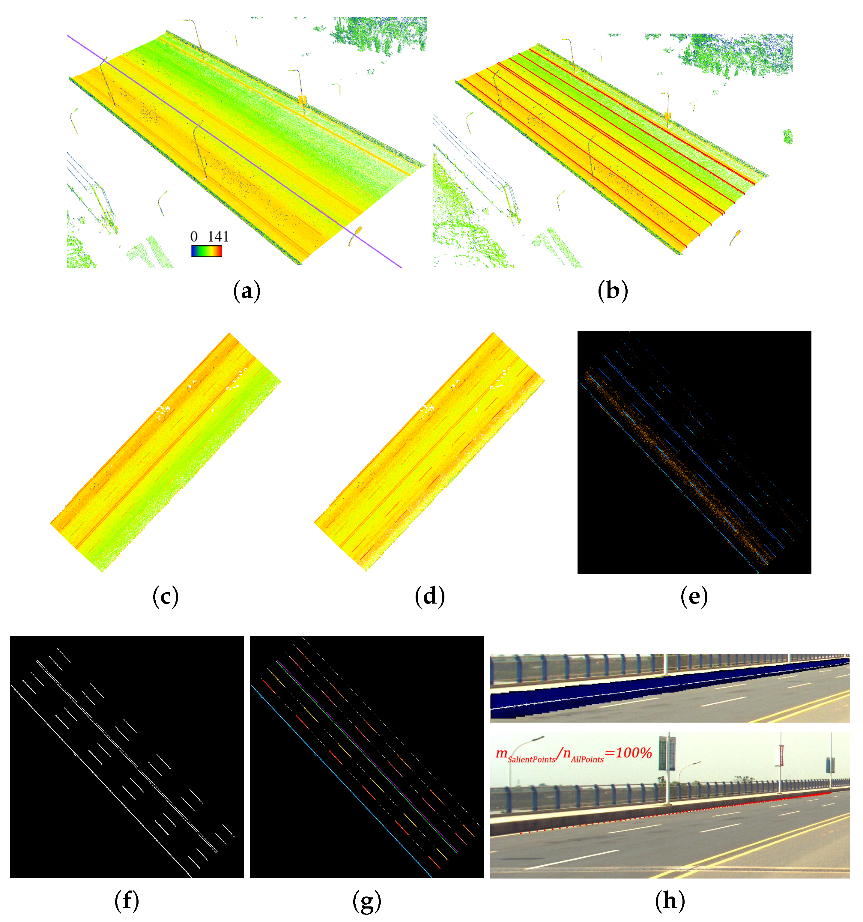
For those road sections that are separated by guardrails, only half of the road is processed. However, for those road sections that are separated by double yellow lines, the lane lines of both sides are extracted. As shown in Figure 20a, the raw data are a two-way six-lane road with roadside walkways, and the purple line is the trajectory. The points far from the trajectory have lower reflective intensity and sparse density, which makes it difficult to extract the lane markings far from the trajectory. Using the proposed method, the pavement is first extracted (Figure 20c). After intensity correction (Figure 20d), the reflective intensity of the points is enhanced. Then, a 2D intensity image is generated (Figure 20e) and segmented using self-adaptive thresholding (Figure 20f). The lane near the road boundary is missed since the points are too sparse. Therefore, the successfully extracted near-vehicle lane is used to infer this lane (the upper right lane in Figure 20g). In addition, textural saliency analysis is used to validate the inferred lane. A group of square buffers are obtained in the MMS image, and the pixels with posterior probability P ( H 1 | F ( x ) ) greater than 0.8 are considered salient, as indicated by the white pixels in the upper picture of Figure 20h. There are 120 valid sampling points of the 120 points, i.e., m / n = 100 % > 50 % ; thus, the inferred lane is considered valid. Finally, the 3D lane lines are obtained, as shown in Figure 20b. For the double yellow lines, we first extract the line that is closer to the trajectory. By analyzing its surroundings, the other line can be obtained.
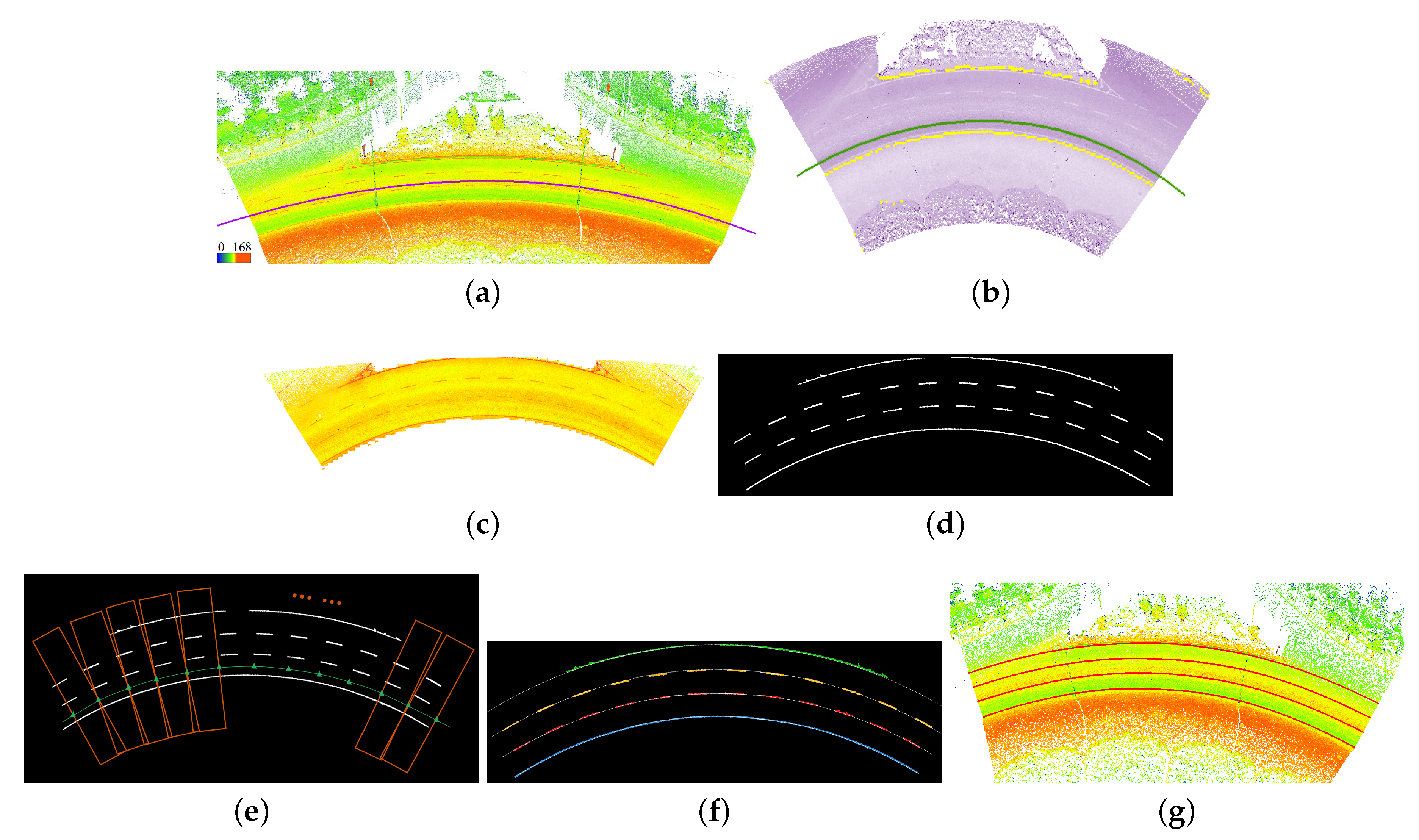
For the curved road as shown in Figure 21a, the proposed method processes the point cloud piecewise based on the line segments between the adjacent trajectory points. The curb grids are first located by searching along the orthogonal direction of these trajectory line segments, as shown in Figure 21b. The pavement points are segmented by the curbs and enhanced by intensity correction (Figure 21c). An intensity image is generated using the pavement points and segmented by self-adaptive thresholding (Figure 21d). Then, along the orthogonal direction of the trajectory line segments, the lane markings’ deviation from the trajectory can be calculated despite the curvature of the road (Figure 21e). Finally, the lane lines are obtained by clustering and fitting the lane-marking pixels (Figure 21f). The 3D lane lines are shown in Figure 21g.

3.3.2. Overall Mapping Results

Figure 22 shows the overall mapping results. The red lines are the inferred lane lines that are considered invalid in the textural saliency analysis. Since they can improve the continuity, they are kept for further manual check but not included in the evaluation. Three typical road types (e.g., straight, curved and roundabout) are selected and overlaid with Google Earth images [Map Data: Google, 2018 DigitalGlobe]. As shown in Figure 23, the lane-level map coincides well with the image, which demonstrates the effectiveness of the proposed method.

3.3.3. Evaluation and Error Analysis

As shown in Table 1, the recall, precision, and F-score of the overall lane mapping reach 96.4%, 97.6% and 97.0%, respectively. The false positives are caused mainly by the complex junction where the roundabout and the three-lane road join each other. An irregular lane with much larger width than that of the standard lanes causes false negatives. The detailed cases will be analyzed below.
As shown by the point cloud (Figure 24a) and the corresponding MMS image (Figure 24b), the junction where the vehicle enters the roundabout is rather complex, which makes it difficult to track the lanes correctly. As shown in Figure 24c, the gray lines are the incorrectly tracked lanes. In an actual project, it is necessary to first locate those junctions and annotate the lane lines manually.
As shown in Figure 25b, a lane approximately 10.5 m wide, which does not meet the standard width that ranges from 3.25 m to 3.75 m, is located at the exit of the roundabout. Although local detection fails to recognize this lane, the global post-processing supplements four lines, two of which are validated by the textural saliency analysis, as shown in Figure 25c. The false positives are meaningful because they can provide a reference for the manual check.

4. Discussion

4.1. Discussion of Textural Saliency Analysis

Textural saliency analysis can be used in many cases, including the long and solid lane markings near the road boundary mentioned in Section 3.3.1, the dashed lane markings near the road boundaries or the center.
For dashed lane markings near the road boundaries, a lane line far from the trajectory is inferred by the near-vehicle lane line, as shown in Figure 26a. The sampling points are mapped to the image and textural saliency analysis is performed in the buffers around each sampling point, as shown in Figure 26b. Two detector windows that contain the lane marking and the pavement are compared, as shown in Figure 26c. Sampling points with salient and linear objects in their buffers are considered valid. There are 38 valid points of the 64 sampling points, and m / n = 59.4 % > 50 % . Therefore, this inferred line is considered valid.
There are cases when the interference is so strong and the contrast between the lane markings and the asphalt road is so weak that the method fails to extract the near-vehicle lane. If only one of the near-vehicle lane lines is successfully extracted, we infer it to obtain the other one. The width of the lane W is decided by the previous road section. As shown in Figure 27a,b, the other near-vehicle lane line is obtained and validated by textural saliency analysis. Since the slope of the near-vehicle line is larger than that of the lane lines near the road boundaries, the shape and size of the detector window are set horizontally as shown in Figure 27c. The border window B is obtained by expanding the left and right of the window K by 25%. In addition, the height of window K is set to 0.5 · w k , where w k is the width of K. After textural saliency analysis, since there are 56 valid points of the 71 sampling points and m / n = 78.9 % , this line is considered valid.

4.2. Discussion of Global Post-Processing

Global post-processing complements the missing lane line points based on global continuity. As shown in Figure 28a, some lane line points are missed in a local road section due to the occlusion of a vehicle. Since the distance between two adjacent lane line points reaches 31.6 m, which is greater than the threshold 20 m (the average length of a road section), the corresponding trajectory points are moved to complement the lane line. After validation with the textural saliency method and global B-spline curve fitting, the complementary line is shown in Figure 28b.

5. Conclusions

Most current studies based on the MMS do not consider the images and only use the point cloud to extract road markings. However, the point becomes very sparse and the quality of reflective intensity deteriorates because of the increase of the range, instrument settings, velocity of the car or the quality of used MMS, which makes it difficult to successfully extract the road markings from the sparse points for those studies. The combined lane mapping method proposed in this paper can effectively solve this problem. First, intensity correction is used to eliminate the intensity inconsistency caused by the range. Then, self-adaptive thresholding of the intensity is developed to extract the lane markings against the impact of the interference. Finally, LiDAR-guided textural saliency analysis is adopted for lane mapping, especially for those lane lines that are far away and difficult to extract by methods that use only point clouds. Global post-processing complements the missing lane lines caused by the occlusion of vehicles and improves the robustness of lane mapping. The test results with the dataset from Wuhan achieved a recall of 96.4%, a precision of 97.6% and an F-score of 97.0%, demonstrating that the proposed method has strong processing ability for complex urban roads.
Future studies can use the prior map to rely less on real-time trajectories and improve the robustness of lane mapping, especially when the measuring vehicle changes lanes. Moreover, an update of the lane-level map that integrates cloud points and images is suggested for further study. A low-cost photogrammetry-based generation of lane-level maps using UAVs and cars is also suggested.

Author Contributions

R.W., Y.H. and R.X. conceived and designed the framework of this research; R.W., R.X. and P.M. performed the experiments; Y.H. supervised this research; R.W., Y.H. and R.X. wrote this paper.

Funding

This research was funded by the Natural Science Foundation of China Project (No. 41671419, No. 51208392), the inter-discplinary research program of Wuhan University (No. 2042017kf0204).

Acknowledgments

The authors would like to gratefully acknowledge Leador Spatial Information Technology Corporation who provided us with the data support.

Conflicts of Interest

The authors declare no conflict of interest.

References

  1. Levinson, J.; Askeland, J.; Becker, J.; Dolson, J.; Held, D.; Kammel, S.; Kolter, J.Z.; Langer, D.; Pink, O.; Pratt, V.; et al. Towards fully autonomous driving: Systems and algorithms. In Proceedings of the 2011 IEEE Intelligent Vehicles Symposium (IV), Baden-Baden, Germany, 5–9 June 2011; pp. 163–168. [Google Scholar]
  2. Urmson, C.; Anhalt, J.; Bagnell, D.; Baker, C.; Bittner, R.; Clark, M.N.; Dolan, J.; Duggins, D.; Galatali, T.; Geyer, C.; et al. Autonomous driving in Urban environments: Boss and the Urban Challenge. J. Field Robot. 2008, 25, 425–466. [Google Scholar] [CrossRef]
  3. Levinson, J.; Montemerlo, M.; Thrun, S. Map-Based Precision Vehicle Localization in Urban Environments. In Proceedings of the Robotics: Science and Systems 2007, Atlanta, GA, USA, 27–30 June 2007; p. 1. [Google Scholar]
  4. Levinson, J.; Thrun, S. Robust vehicle localization in urban environments using probabilistic maps. In Proceedings of the 2010 IEEE International Conference on Robotics and Automation, Anchorage, AK, USA, 3–8 May 2010; pp. 4372–4378. [Google Scholar]
  5. Tao, Z.; Bonnifait, P.; Fremont, V.; Ibañez-Guzman, J. Mapping and localization using GPS, lane markings and proprioceptive sensors. In Proceedings of the IEEE/RSJ International Conference on Intelligent Robots and Systems (IROS 2013), Tokyo, Japan, 3–7 November 2013; pp. 406–412. [Google Scholar]
  6. Schreiber, M.; Knoppel, C.; Franke, U. LaneLoc: Lane Marking based Localization using Highly Accurate Maps. In Proceedings of the 2013 IEEE Intelligent Vehicles Symposium (IV), Gold Coast, Australia, 23–26 June 2013; pp. 449–454. [Google Scholar]
  7. Gu, Y.; Wada, Y.; Hsu, L.; Kamijo, S. Vehicle self-localization in urban canyon using 3D map based GPS’ positioning and vehicle sensors. In Proceedings of the 2014 International Conference on Connected Vehicles and Expo (ICCVE), Vienna, Austria, 3–7 November 2014; pp. 792–798. [Google Scholar]
  8. Oliver, N.; Pentland, A.P. Driver Behavior Recognition and Prediction in a SmartCar. Proc. SPIE 2015, 4023, 280–290. [Google Scholar]
  9. Doshi, A.; Trivedi, M.M. Tactical driver behavior prediction and intent inference: A review. In Proceedings of the 14th Internetional IEEE Conference on Intelligent Transpotation Systems, Washinton, DC, USA, 5–7 October 2011; pp. 1892–1897. [Google Scholar]
  10. Ziegler, J.; Bender, P.; Schreiber, M.; Lategahn, H.; Strauss, T.; Stiller, C.; Dang, T.; Franke, U.; Appenrodt, N.; Keller, C.G.; et al. Making bertha drive-an autonomous journey on a historic route. IEEE Intell. Transp. Syst. Mag. 2014, 6, 8–20. [Google Scholar] [CrossRef]
  11. Li, X.; Sun, Z.; Cao, D.; He, Z.; Zhu, Q. Real-Time Trajectory Planning for Autonomous Urban Driving: Framework, Algorithms, and Verifications. IEEE/ASME Trans. Mechatron. 2016, 21, 740–753. [Google Scholar] [CrossRef]
  12. Rogers, S. Creating and evaluating highly accurate maps with probe vehicles. In Proceedings of the 2000 IEEE Intelligent Transportation Systems, Dearborn, MI, USA, 1–3 October 2000; pp. 125–130. [Google Scholar] [Green Version]
  13. Betaille, D.; Toledo-Moreo, R. Creating enhanced maps for lane-level vehicle navigation. IEEE Trans. Intell. Transp. Syst. 2010, 11, 786–798. [Google Scholar] [CrossRef]
  14. Chen, A.; Ramanandan, A.; Farrell, J.A. High-precision lane-level road map building for vehicle navigation. In Proceedings of the IEEE/ION Position, Location and Navigation Symposium, Indian Wells, CA, USA, 4–6 May 2010; pp. 1035–1042. [Google Scholar]
  15. Schindler, A.; Maier, G.; Janda, F. Generation of high precision digital maps using circular arc splines. In Proceedings of the 2012 IEEE Intelligent Vehicles Symposium, Alcala de Henares, Spain, 3–7 June 2012; pp. 246–251. [Google Scholar]
  16. Biagioni, J.; Eriksson, J. Inferring Road Maps from Global Positioning System Traces. Transp. Res. Rec. J. Transp. Res. Board 2012, 2291, 61–71. [Google Scholar] [CrossRef]
  17. Sehestedt, S.; Kodagoda, S.; Alempijevic, A.; Dissanayake, G. Efficient Lane Detection and Tracking in Urban Environments. In Proceedings of the 3rd European Conference on Mobile Robots, Freiburg, Germany, 19–21 September 2007; pp. 78–83. [Google Scholar]
  18. Aly, M. Real time detection of lane markers in urban streets. In Proceedings of the 2008 IEEE Intelligent Vehicles Symposium, Eindhoven, The Netherlands, 4–6 June 2008; pp. 7–12. [Google Scholar]
  19. Borkar, A.; Hayes, M.; Smith, M.T. Robust lane detection and tracking with Ransac and Kalman filter. In Proceedings of the 2009 16th IEEE International Conference on Image Processing (ICIP), Cairo, Egypt, 7–10 November 2009; pp. 3261–3264. [Google Scholar]
  20. Borkar, A.; Hayes, M.; Smith, M.T. A novel lane detection system with efficient ground truth generation. IEEE Trans. Intell. Transp. Syst. 2012, 13, 365–374. [Google Scholar] [CrossRef]
  21. Bar Hillel, A.; Lerner, R.; Levi, D.; Raz, G. Recent progress in road and lane detection: A survey. Mach. Vis. Appl. 2014, 25, 727–745. [Google Scholar] [CrossRef]
  22. Nedevschi, S.; Oniga, F.; Danescu, R.; Graf, T.; Schmidt, R. Increased Accuracy Stereo Approach for 3D Lane Detection. In Proceedings of the 2006 IEEE Intelligent Vehicles Symposium, Tokyo, Japan, 13–15 June 2006; pp. 42–49. [Google Scholar]
  23. Petrovai, A.; Danescu, R.; Nedevschi, S. A stereovision based approach for detecting and tracking lane and forward obstacles on mobile devices. In Proceedings of the IEEE Intelligent Vehicles Symposium, Seoul, Korea, 28 June–1 July 2015; pp. 634–641. [Google Scholar]
  24. Nex, F.; Remondino, F. UAV for 3D mapping applications: A review. Appl. Geomat. 2014, 6, 1–15. [Google Scholar] [CrossRef]
  25. Colomina, I.; Molina, P. ISPRS Journal of Photogrammetry and Remote Sensing Unmanned aerial systems for photogrammetry and remote sensing: A review. ISPRS J. Photogramm. Remote Sens. 2014, 92, 79–97. [Google Scholar] [CrossRef]
  26. Barber, D.; Mills, J.; Smith-Voysey, S. Geometric validation of a ground-based mobile laser scanning system. ISPRS J. Photogramm. Remote Sens. 2008, 63, 128–141. [Google Scholar] [CrossRef]
  27. Puente, I.; González-Jorge, H.; Martínez-Sánchez, J.; Arias, P. Review of mobile mapping and surveying technologies. Measurement 2013, 46, 2127–2145. [Google Scholar] [CrossRef]
  28. Li, R. Mobile Mapping: An Emerging Technology for Spatial Data Acquisition. Photogramm. Eng. Remote Sens. 1997, 63, 1085–1092. [Google Scholar]
  29. Ma, L.; Li, Y.; Li, J.; Wang, C.; Wang, R.; Chapman, M.A. Mobile laser scanned point-clouds for road object detection and extraction: A review. Remote Sens. 2018, 10, 1531. [Google Scholar] [CrossRef]
  30. Ogawa, T.; Takagi, K. Lane Recognition Using On-vehicle LIDAR. In Proceedings of the 2006 IEEE Intelligent Vehicles Symposium, Tokyo, Japan, 13–15 June 2006; pp. 540–545. [Google Scholar]
  31. Smadja, L.; Ninot, J.; Gavrilovic, T. Road extraction and environment interpretation from Lidar sensors. IAPRS 2010, 38, 281–286. [Google Scholar]
  32. Hanyu, W.; Huan, L.; Chenglu, W.; Jun, C.; Peng, L.; Yiping, C.; Cheng, W.; Jonathan, L. Road Boundaries Detection Based on Local Normal Saliency from Mobile Laser Scanning Data. IEEE Geosci. Remote Sens. Lett. 2015, 12, 2085–2089. [Google Scholar] [CrossRef]
  33. Rodríguez-Cuenca, B.; García-Cortés, S.; Ordóñez, C.; Alonso, M.C. An approach to detect and delineate street curbs from MLS 3D point cloud data. Autom. Constr. 2015, 51, 103–112. [Google Scholar] [CrossRef]
  34. Weiss, T. Automatic detection of traffic infrastructure objects for the rapid generation of detailed digital maps using laser scanners. In Proceedings of the 2007 Intelligent Vehicles Symposium, Istanbul, Turkey, 13–15 June 2007; pp. 1271–1277. [Google Scholar]
  35. Boyko, A.; Funkhouser, T. Extracting roads from dense point clouds in large scale urban environment. ISPRS J. Photogramm. Remote Sens. 2011, 66, S2–S12. [Google Scholar] [CrossRef] [Green Version]
  36. Zhao, G.; Yuan, J. Curb detection and tracking using 3D-LIDAR scanner. In Proceedings of the 2012 19th IEEE International Conference on Image Processing, Orlando, FL, USA, 30 September–3 October 2012; pp. 437–440. [Google Scholar]
  37. Wang, H.; Cai, Z.; Luo, H.; Wang, C.; Li, P.; Yang, W.; Ren, S.; Li, J. Automatic road extraction from mobile laser scanning data. In Proceedings of the 2012 International Conference on Computer Vision in Remote Sensing, Xiamen, China, 16–18 December 2012; pp. 136–139. [Google Scholar]
  38. Toth, C.; Paska, E.; Brzezinska, D. Using Road Pavement Markings as Ground Control for LiDAR Data. Int. Arch. Photogramm. Remote Sens. Spat. Inf. Sci. 2008, 37, 189–195. [Google Scholar]
  39. Hata, A.; Wolf, D. Road marking detection using LIDAR reflective intensity data and its application to vehicle localization. In Proceedings of the 17th International IEEE Conference on Intelligent Transportation Systems (ITSC), Qingdao, China, 8–11 October 2014; pp. 584–589. [Google Scholar]
  40. Chen, X.; Kohlmeyer, B.; Stroila, M.; Alwar, N.; Wang, R.; Bach, J. Next generation map making. In Proceedings of the 17th ACM SIGSPATIAL International Conference on Advances in Geographic Information Systems, Seattle, WA, USA, 4–6 Novermber 2009; pp. 488–491. [Google Scholar]
  41. Kumar, P.; McElhinney, C.P.; Lewis, P.; McCarthy, T. Automated road markings extraction from mobile laser scanning data. Int. J. Appl. Earth Obs. Geoinf. 2014, 32, 125–137. [Google Scholar] [CrossRef] [Green Version]
  42. Guan, H.; Li, J.; Yu, Y.; Wang, C.; Chapman, M.; Yang, B. Using mobile laser scanning data for automated extraction of road markings. ISPRS J. Photogramm. Remote Sens. 2014, 87, 93–107. [Google Scholar] [CrossRef]
  43. Soilán, M.; Riveiro, B.; Martínez-Sánchez, J.; Arias, P. Segmentation and classification of road markings using MLS data. ISPRS J. Photogramm. Remote Sens. 2017, 123, 94–103. [Google Scholar] [CrossRef]
  44. Yu, Y.; Li, J.; Guan, H.; Jia, F.; Wang, C. Learning Hierarchical Features for Automated Extraction of Road Markings From 3-D Mobile LiDAR Point Clouds. IEEE J. Sel. Top. Appl. Earth Obs. Remote Sens. 2015, 8, 709–726. [Google Scholar] [CrossRef]
  45. Ishikawa, K.; Takiguchi, J.I.; Amano, Y.; Hashizume, T. A mobile mapping system for road data capture based on 3D road model. In Proceedings of the IEEE International Conference on Control Applications, Munich, Germany, 4–6 October 2007; pp. 638–643. [Google Scholar]
  46. Hůlková, M.; Pavelka, K.; Matoušková, E. Automatic classification of point clouds for highway documentation. Acta Polytech. 2018, 58, 165–170. [Google Scholar] [CrossRef]
  47. Huang, P.; Cheng, M.; Chen, Y.; Luo, H.; Wang, C.; Li, J. Traffic Sign Occlusion Detection Using Mobile Laser Scanning Point Clouds. IEEE Trans. Intell. Transp. Syst. 2017, 18, 2364–2376. [Google Scholar] [CrossRef]
  48. Hu, X.; Rodriguez, F.S.A.; Gepperth, A. A multi-modal system for road detection and segmentation. In Proceedings of the 2014 IEEE Intelligent Vehicles Symposium, Dearborn, MI, USA, 8–11 June 2014; pp. 1365–1370. [Google Scholar]
  49. Xiao, L.; Dai, B.; Liu, D.; Hu, T.; Wu, T. CRF based road detection with multi-sensor fusion. In Proceedings of the 2015 IEEE Intelligent Vehicles Symposium (IV), COEX, Seoul, Korea, 28 June–1 July 2015; pp. 192–198. [Google Scholar]
  50. Premebida, C.; Carreira, J.; Batista, J.; Nunes, U. Pedestrian detection combining RGB and dense LIDAR data. In Proceedings of the 2014 IEEE/RSJ International Conference on Intelligent Robots and Systems, Chicago, IL, USA, 14–18 September 2014; pp. 4112–4117. [Google Scholar]
  51. Schoenberg, J.R.; Nathan, A.; Campbell, M. Segmentation of dense range information in complex urban scenes. In Proceedings of the 2010 IEEE/RSJ International Conference on Intelligent Robots and Systems, Taipei, Taiwan, 18–21 October 2010; pp. 2033–2038. [Google Scholar]
  52. Tan, K.; Cheng, X.; Ding, X.; Zhang, Q. Intensity Data Correction for the Distance Effect in Terrestrial Laser Scanners. IEEE J. Sel. Top. Appl. Earth Obs. Remote Sens. 2016, 9, 304–312. [Google Scholar] [CrossRef]
  53. Rahtu, E.; Heikkila, J. A Simple and efficient saliency detector for background subtraction. In Proceedings of the 2009 IEEE 12th International Conference on Computer Vision Workshops, Kyoto, Japan, 27 September–4 October 2009; pp. 1137–1144. [Google Scholar]
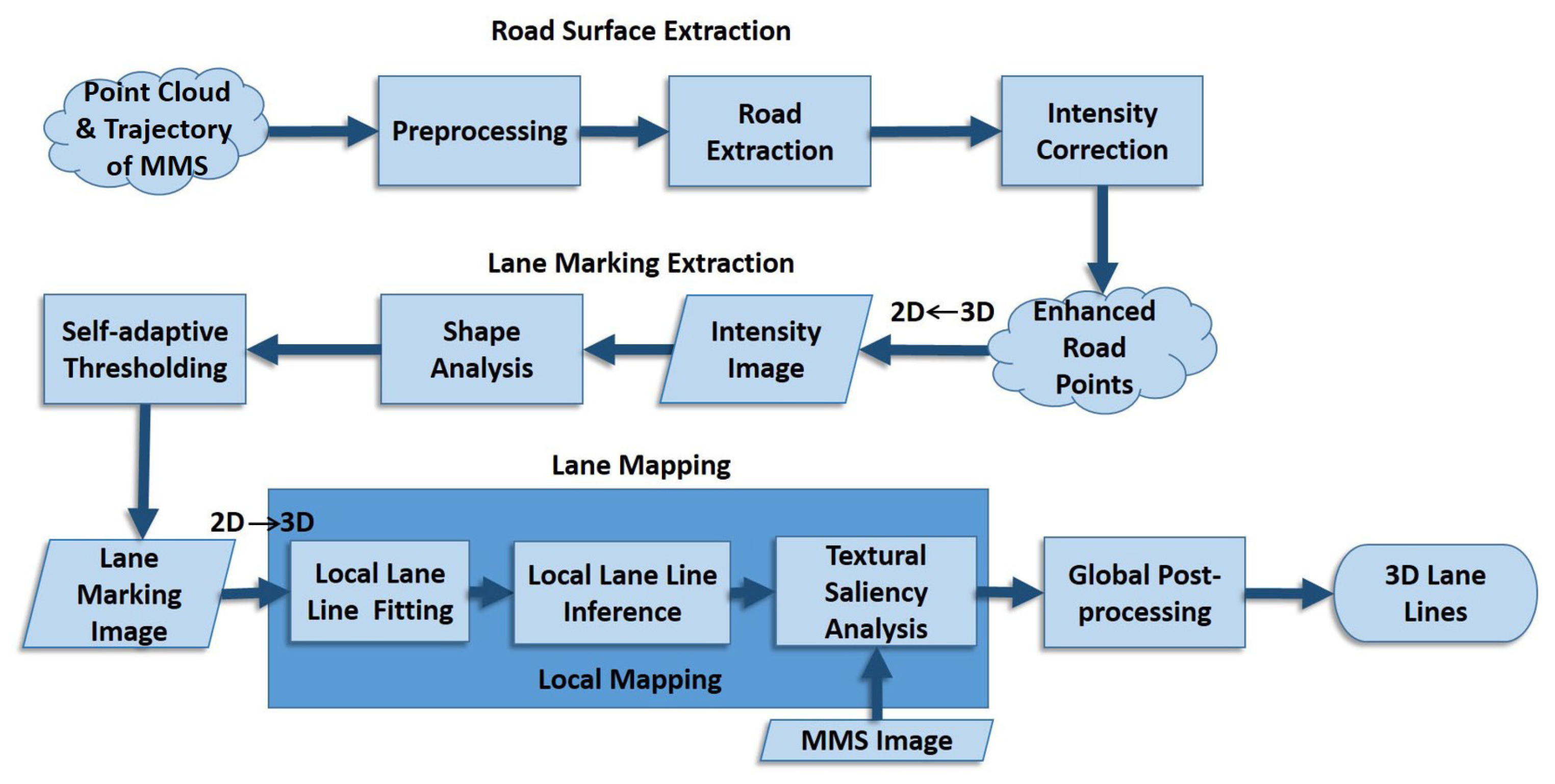
Figure 1. Overview of the method.
Remotesensing 11 00305 g001
Figure 2. The raw point cloud data contains massive amounts of irrelevant data.
Remotesensing 11 00305 g002
Figure 3. Preprocessing based on the trajectory. The blue arrow indicates the trajectory, and the green arrow is perpendicular to the trajectory. The points outside the red line, whose distance to the trajectory is greater than W t , will be removed.
Remotesensing 11 00305 g003
Figure 4. Preprocessing based on elevation. (a) First, an elevation histogram in meters is plotted, and the pavement elevation is 9 m. (b) Then, a further elevation histogram in decimeters is plotted, and the pavement elevation is 9.5 m. (c,d) The point cloud before and after elevation-based removal.
Remotesensing 11 00305 g004
Figure 5. 3D points are assigned to the corresponding grids based on their X and Y coordinates. The red line is the trajectory. Along the arrow that indicates the orthogonal direction of the trajectory, the curbs are searched for.
Remotesensing 11 00305 g005
Figure 6. (a) The yellow points present the result of the search for curb grids. The red box indicates the vehicle points that are incorrectly recognized as curbs. (b) The colored points are the retained road points, and the gray points are the removed points. The precise road is obtained, and the vehicles are removed.
Remotesensing 11 00305 g006
Figure 7. Intensity correction. The color indicates the intensity value and the blue arrow indicates the trajectory. For each point, R is the distance from the point to the trajectory line. (a) The uncorrected road points. The intensity of the points far from the trajectory is significantly lower. (b) The corrected road points. The impact of the range on intensity is reduced, while the reflective intensity contrast between lane markings and the pavement is highlighted.
Remotesensing 11 00305 g007
Figure 8. (a) The threshold is too low and leads to considerable noise. (b) The threshold is too high and leads to incomplete extraction.
Remotesensing 11 00305 g008
Figure 9. The correspondence between the 3D point cloud and the 2D images. On the left is a top view of the 3D point cloud, whose origin is at the lower-left corner. On the right are the generated 2D intensity and elevation images, whose origins are at the upper-left corner. The gray values of the pixel ( x p , y p ) in the 2D intensity and elevation images are equal to the intensity and elevation of the 3D point ( X p , Y p , Z P ) , respectively.
Remotesensing 11 00305 g009
Figure 10. (a) The orange part is the interference region. (b) The orange part is dimmed compared with (a), which means that interference is suppressed. (c) The extracted lane markings.
Remotesensing 11 00305 g010
Figure 11. (a) A binary image with a zebra crossing. (b) After a closing operation, the zebra crossing is connected to a rectangle whose long axis is nearly perpendicular to the trajectory. (c) A binary image with a stop line. (d) After an opening operation, the stop line is separated into several rectangles whose long axes are nearly perpendicular to the trajectory. (e) The stop line is removed. (f) A binary image with straight-ahead arrows and diamond markings. (g) The false positive markings are removed through shape analysis.
Remotesensing 11 00305 g011
Figure 12. (a) The white pixels are the skeletonized lane markings. The red triangles are the trajectory points, and they are connected by line segment L i . The green boxes represent the moving buffer B i . The purple line indicates the change in s with respect to d of B i . In addition, the two orange boxes are the peak buffers P j i ( j = 1 , 2 ) . (b) Each colored polyline represents the change in s with respect to d of each B i ( i = 1 , 2 , , n - 1 ) . In the figure, two groups are formed as indicated by the red ellipses, and the pixels in the peak buffers of a group are on the same lane line.
Remotesensing 11 00305 g012
Figure 13. The process of buffer-analysis-based lane line inference. The purple continuous line is the trajectory, while the green line is the right host lane line. The green line is moved parallel to the right, and white pixels are searched for in a buffer that ranges from W - 0.5 m to W + 0.5 m, as indicated by the orange area. The blue line that matches the white pixels best is selected as the candidate lane line.
Remotesensing 11 00305 g013
Figure 14. The 3D points are mapped onto the MMS image plane. (a) The relationship between the geodetic, IMU, and camera coordinate systems. (b) From the camera coordinate system to the MMS image plane, we finally obtain the column and row of the mapped pixel.
Remotesensing 11 00305 g014
Figure 15. An example of mapping a candidate lane line. (a) In the colored point cloud, the blue line is a candidate lane line while the pink box is the 1m wide buffer. (b) The green box is the mapped buffer guided by the LiDAR geometry.
Remotesensing 11 00305 g015
Figure 16. A case of textural saliency analysis. (a) The green box is a square buffer around the sampling point. After the textural saliency analysis of each buffer, there are 39 salient points (red), and 31 points that are not salient (blue). The lane line in this picture is valid since m / n > 50 % . (b) A detector window is divided into the kernel window K and the border window B, which are marked with a red border. The pictures in the middle are the distribution of pixels in windows B and K, the contrast of which determines the saliency. On the right is the saliency value in the window. (c) The grayscale histograms in the green, yellow, orange and blue regions are denoted w 1 , w 2 , w 3 , w 4 , respectively, which are also the values of the four corners of the red region in the integral histogram. The gray value histogram in the red region can be quickly calculated by w 1 + w 4 - w 2 - w 3 . (d) The saliency values in the buffer in (a) after thresholding.
Remotesensing 11 00305 g016
Figure 17. Complementing with missing points. The blue line is the correct lane line. Point A is the trajectory point that corresponds to the blue line, and point B is the trajectory point that corresponds to the missing line. By drawing a line perpendicular to A B through point A, this line intersects the blue line at point C. The distance d of A C is calculated, and point B is moved distance d along the orthogonal direction of A B to point D, which is the complementary lane line point.
Remotesensing 11 00305 g017
Figure 18. Experimental data. Trajectories in the Jiangxia District in the city of Wuhan.
Remotesensing 11 00305 g018
Figure 19. A three-lane road section. (a) The raw data. The color from blue to red indicates the intensity from low to high. The purple line is the trajectory and the red dotted lines are the road edges. (b) The 3D lane lines are presented in the colored point cloud. (c) The road points that are segmented by the edges. (d) The road points after intensity correction. (e) The 2D intensity image. The blue parts are the road markings while the orange part is the interference. (f) The binary image that contains all the road markings. (g) The binary image that contains only the lane markings. (h) The lane-marking pixels are clustered into groups and each group is marked by a unique color. The white lines are the fitted lane lines.
Remotesensing 11 00305 g019
Figure 20. A two-way six-lane road section. (a) The raw data. The purple line is the trajectory. (b) The red 3D lane lines are presented in the colored point cloud. (c) The road points. (d) The road points after intensity correction. (e) The intensity image. The blue part is the lane markings and the orange part is the interference. (f) The binary image. (g) The colors indicate the groups of the clustered lane-marking pixels. The white lines are the lane lines fitted from the pixels of each group. (h) The textural saliency analysis. The upper picture shows the saliency values of the buffers around each sampling point. In the lower picture, the red points are the salient sampling points.
Remotesensing 11 00305 g020
Figure 21. A roundabout road section. (a) The raw data. The purple line is the trajectory. (b) The road extraction. The yellow points are the curb grids and the green line is the trajectory. (c) The road points. (d) The binary image. (e) The process of clustering. The green triangles are the trajectory points and are connected sequentially to form line segments. Along the orange boxes that are perpendicular to each line segment, the deviation of every lane-marking pixel can be calculated. (f) The lane-marking pixels of each group are marked by a unique color, and the white lines are the lane lines fitted from those pixels. (g) The red 3D lane lines are presented in the colored point cloud.
Remotesensing 11 00305 g021
Figure 22. The overall mapping results.
Remotesensing 11 00305 g022
Figure 23. The mapping results are overlaid with Google Earth images in (a) a straight road section, (b) a curved road section, and (c) the roundabout.
Remotesensing 11 00305 g023
Figure 24. Error analysis: the junction. (a) The raw data of a junction where the vehicle enters the roundabout. (b) The corresponding MMS image. (c) The mapping result is presented in the colored point cloud, where the correct extractions are red, and the false positives are gray.
Remotesensing 11 00305 g024
Figure 25. Error analysis: the irregular lane. (a) The raw data with a 10.5 m wide lane. (b) The corresponding MMS image. (c) Four lines are obtained by global post-processing. Correct extractions are red, and the false positives are gray.
Remotesensing 11 00305 g025
Figure 26. Textural saliency analysis of the dashed lane markings near the road boundary. (a) The dotted purple line is the trajectory, and the red line is the inferred lane line. (b) The lower picture shows the inferred line that is sampled and mapped onto the image. Through textural saliency analysis, valid sampling points are marked in red and invalid ones are marked in blue. The upper picture presents the saliency values of the buffers around each sampling point. The green box is a buffer of a valid sampling point. (c) Two detector windows and their saliency values are shown on the left. The contrast of the K and B windows, whose distributions of the gray values are shown on the right, decides the saliency values.
Remotesensing 11 00305 g026
Figure 27. Textural saliency analysis for near-vehicle lane markings. (a) The dotted purple line is the trajectory, and the red line is the inferred lane line. (b) The inferred lane line is sampled and mapped to the image, as shown on the right. Through textural saliency analysis, the valid points are marked in red and the invalid ones are marked in blue. The saliency values of the buffers around the sampling points are shown on the left. (c) In the buffer denoted by the green box in (b) the detector window is shown on the left and the saliency map on the right.
Remotesensing 11 00305 g027
Figure 28. A case of global post-processing for complementing the missing lane line. (a) The map before global post-processing. The lane line in a road section is missed due to the occlusion of a vehicle. The dotted purple line is the trajectory, and the red lines are the correctly extracted lane lines before and after this road section. (b) The blue line is the complementary lane line
Remotesensing 11 00305 g028
Table 1. Lane mapping results.
  TP /m FN /m FP /m Recall Precise F score
six-lane road3302.6546.9942.030.9860.9870.987
roundabout309.9888.1148.580.7790.8650.819
overall3612.63135.1090.610.9640.9760.970