Abstract
Hyperspectral image (HSI) change detection plays an important role in remote sensing applications, and considerable research has been done focused on improving change detection performance. However, the high dimension of hyperspectral data makes it hard to extract discriminative features for hyperspectral processing tasks. Though deep convolutional neural networks (CNN) have superior capability in high-level semantic feature learning, it is difficult to employ CNN for change detection tasks. As a ground truth map is usually used for the evaluation of change detection algorithms, it cannot be directly used for supervised learning. In order to better extract discriminative CNN features, a novel noise modeling-based unsupervised fully convolutional network (FCN) framework is presented for HSI change detection in this paper. Specifically, the proposed method utilizes the change detection maps of existing unsupervised change detection methods to train the deep CNN, and then removes the noise during the end-to-end training process. The main contributions of this paper are threefold: (1) A new end-to-end FCN-based deep network architecture for HSI change detection is presented with powerful learning features; (2) An unsupervised noise modeling method is introduced for the robust training of the proposed deep network; (3) Experimental results on three datasets confirm the effectiveness of the proposed method.
1. Introduction
Hyperspectral images (HSIs) acquired by hyperspectral imaging sensors have been available for research since the early 1980s [1]. Because of the hundreds of nearly continuous spectra, HSIs help to distinguish the subtle differences of various ground objects [2]. The rich spectral information found in HSIs makes them useful in many applications, such as band selection [3,4,5], anomaly detection [6,7,8], image classification [9,10,11], hyperspectral unmixing [12,13,14,15], change detection [16,17,18,19], and so on. Among them, HSI change detection provides a timely and powerful means to observe our changing planet, which is a very significant study. To be specific, change detection is the process of identifying the differences of the same ground objects by observing them at different times [20]. Its use in various geologic applications is well documented, for example in the fields of disaster monitoring [21], resource and environment management [22,23], and land cover mapping [24,25]. In general, there are three main steps for a complete HSI change detection, namely, image preprocessing, change detection map generation, and evaluation. Among these steps, how to generate the final change detection map is the most important problem for change detection research.
Many change detection methods have been proposed in recent years. Simple methods to generate change detection maps are image subtraction and the use of ratios and other mathematical operators. The results of these operations are used by different segmentation and classification methods. The most common method is change vector analysis (CVA) [26],which is a typically unsupervised method using spectral vector subtraction. Additionally, some modified CVA methods are presented in References [27,28,29,30]. In Reference [31], a hybrid vector was constructed using a change vector and spectral angle, and then a change detection map was generated using the adaptive fusion strategy. Robust change vector analysis (RCVA) [32] was another improvement of CVA, which was presented to account for the pixel neighborhood effect. In addition to the above, there are other methods based on image transformation. Multivariate alteration detection (MAD) [33] was designed to detect change pixels by exploring canonical correlation analysis. Then, iteratively reweighted MAD (IR-MAD) [34] was developed with different weights for certain observations. In addition, Liu et al. [35] used band selection to select the most informative band subset to address the change detection problem. Shao et al. [36] presented a semi-supervised fuzzy C-means (RSFCM) clustering algorithm, which introduced pseudo-labels from difference images. Wu et al. [37] utilized kernel slow feature analysis and post-classification fusion for scene change detection, which accurately determined the changes. Ertürk et al. [38] tackled the change detection problem by exploring the sparse unmixing based on spectral libraries, which provided subpixel-level change information. Yuan et al. [39] proposed a novel semi-supervised distance metric learning method and detected the change areas by spectral feature.
However, with the development of new imaging sensors [40,41], some traditional change detection methods cannot get satisfactory results in terms of the increasing dimensions of the data. HSIs, characterized by very high spectral resolution, have a greater ability to detect finer changes than other traditional remote sensing images. Despite the methods of change detection being constantly updated, there are still a lot of challenges in HSI change detection task. One challenge is that HSIs are easily influenced by noise during the image acquisition process. Thus, the low level representations of HSIs are not discriminative enough for the task of change detection, which makes it difficult to detect change areas accurately for traditional methods. Another challenge is that the hundreds of spectral bands further make HSIs have an extremely high dimensionality. It is difficult to deal with the high-dimensionality problem for conventional methods. These aforementioned problems need to be addressed to improve the change detection performance. Fortunately, the development of deep learning is a promising way of solving these issues.
Nowadays, the rapid development of deep learning has swept across the field of image analysis due to its powerful learning ability [42,43]. Specifically, deep learning has a powerful tool to deal with the problem of high dimension and feature extraction. However, as a result of the characteristics of HSI change detection and the limited number of datasets, it is difficult to train the whole neural network with ground truth label information. In other words, most available works on deep learning for HSI change detection are trained with pseudo-training sets, which are not real labeled training sets. Therefore, the current studies focused on the application of deep learning related to HSI change detection are still insufficient.
The change detection task based on deep learning can be mainly divided into the following three categories. Firstly, change detection is considered as a binary classification task, which is a supervised method. In other words, the whole network is trained with pseudo-training sets. In this respect, a general end-to-end 2-D convolutional neural network (CNN) framework (GETNET) [44] was presented, aiming at learning features from multi-source data at a higher level. In this work, pseudo-training sets obtained by other change detection methods are necessary to train the whole network. However, the inherent noise in the pseudo-training sets will lead to performance degradation of the algorithms. Secondly, a deep network is trained in an unsupervised way without a priori labels. Gong et al. [45] proposed a discriminative feature learning method for change detection based on a restricted Boltzmann machine (RBM). The two images are transformed into feature spaces and then comparisons of paired features are made to generate the final change detection map. Nevertheless, these networks do not have the strong learning ability of feature extraction like CNN, which weakens the representation of features. Thirdly, pretrained networks on other classification datasets are used for change detection in an unsupervised way. Pretrained CNN was employed to extract features of zooming levels [46] and these concatenated features were compared to obtain the change results. However, the features extracted from pretrained CNN designed for other datasets are suboptimal for the task of change detection. Furthermore, Kevin et al. [47] utilized the CNN model pretrained for semantic segmentation to detect change areas in an unsupervised way. However, this work heavily depends on the ability of a trained model to perform semantic segmentation. In other words, this method becomes invalid when the datasets do not contain segmentation labels.
Additionally, the number of change detection datasets is very limited because it is labor-intensive and time-consuming to label each pixel in an HSI. Despite the fact that there are supervised methods, some of them are based on the pseudo-training datasets which are not real labeled data. However, the unsupervised methods are usually independent of datasets and have more practical applications. The unsupervised learning does not need any labeled data and is able to be applied under various conditions. This, therefore, raises the question: how to learn the change detection map based on deep learning without labeled data while obtaining competitive results with supervised methods.
Considering these problems, how to effectively utilize the rich spectra information in high dimensionality and distinguish useful information from noise in an unsupervised way is an important field of research [15,48,49,50]. In this work, a novel perspective on noise modeling-based unsupervised fully convolutional network (FCN) framework for HSI change detection task is proposed. The proposed end-to-end framework learns the latent change detection map by excluding the noise in change detection maps of existing unsupervised methods. We consider how to improve the performance by the training of the FCN without labeled data in order to obtain the final change detection map. To this end, this paper develops a novel end-to-end unsupervised framework, consisting of three modules: the FCN-based feature learning module, the two-stream feature fusion module, and the unsupervised noise modeling module. These three modules work natively to jointly improve the change detection accuracy. To sum up, the main contributions of this work can be summarized as follows.
- (1)
- A new FCN-based deep network architecture is designed to learn powerful features for the task of change detection. The proposed architecture works in an end-to-end manner, which minimizes the final change detection cost function to avoid error accumulation.
- (2)
- An unsupervised noise modeling module is introduced for the robust training of the proposed deep network in the task of HSI change detection. By excluding the noise in an unsupervised way, the performance is improved effectively.
- (3)
- Extensive experimental results on three datasets demonstrate the proposed method’s superior performance. It not only achieves a better performance than common unsupervised approaches, but is also competitive with some supervised approaches.
2. Methodology
In this section, we introduce the proposed unsupervised HSI change detection framework in detail. As illustrated in Figure 1, the proposed method consists of three main modules. The first one is the FCN-based feature learning module, which is designed to learn discriminative features from high-dimensional data. As HSI change detection is treated as a segmentation task, we propose to employ the FCN-based deep learning framework as the backbone. The second one is the two-stream feature fusion module, which paves the way to feature fusion of two types of data. Different from traditional image classification, the task of change detection involves two HSIs, and how to fuse the two-stream features is still an open problem. The final one is the unsupervised noise modeling module, applied to tackle the influence of the noise and the robust training of the proposed network. The traditional unsupervised change detection method is utilized for excluding the noise by performing this module. After these three modules, the final change detection map is obtained and the accuracy is also improved. The proposed three modules will be described in the following sections.
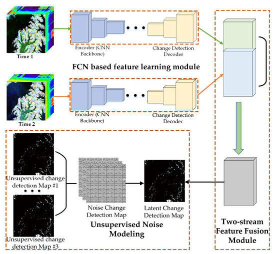
Figure 1.
The illustration of the proposed change detection framework, which consists of an fully convolutional network (FCN)-based feature learning module, a two-stream feature fusion module, and an unsupervised noise modeling module.
2.1. FCN-Based Feature Learning Module
Deep CNN-based HSI change detection methods usually sample patches for feature extraction and classification. However, patch-wise training and testing are not efficient and have extra pre- and post-processing complications. Since change detection requires one to assign labels to all pixels of the input HSIs, it is an essential segmentation task. Inspired by this, we propose to design an unsupervised FCN-based HSI change detection framework.
To clearly present the proposed FCN-based network architecture, we introduce the convolution and deconvolution layers first. Convolution is a basic feature learning component of CNN, which operates on local input regions. Suppose the input data is , and is the spatial coordinate. Then, the convolution output is computed by
where s is the convolution stride and k is the kernel size. is the specific operation for the layer, and for convolution it is a matrix multiplication. Then, the output will be the input of the next layer. By stacking these convolution layers, high semantic-level features are extracted. For a convolution layer, if stride s is set to 2, then the spatial size of the output will be half of the input size. Deconvolution is a special kind of convolution layer, also named transposed convolution, which is used to enlarge the output spatial size. As the weight of the deconvolution layer is transposed, the output spatial size will be two times that of the input size if stride s is set to 2.
The FCN architecture of the proposed work is illustrated in Figure 2 in detail, which consists of an encoder module and a decoder module. On the one hand, convolution layers are used in the encoder module to get the quintessence from original data. On the other hand, deconvolution layers are exploited in the decoder module to recover the input spatial size. We also compare the FCN-based change detection architecture with the patch-wise CNN change detection method. No pre- or post-processing are needed in the FCN-based framework and it can be trained in an end-to-end manner.
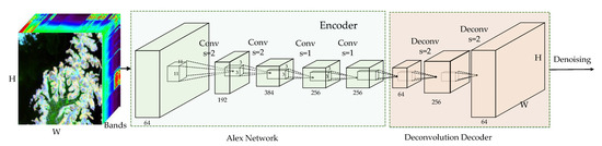
Figure 2.
Architecture of the proposed FCN-based network.
In change detection task, the two HSIs are captured at the same position but different times. Thus, the same FCN-based networks are employed to extract the deep features to make sure that the features of two HSIs are in the same space. Considering and as two input HSIs, the feature extraction of them with the FCN-based network can be formulated as
where and are the encoder network and decoder networks, respectively. The final convolution feature maps of the two input HSIs are denoted as and , which are used for the following feature fusion module. N is the batch size, and C is the channel size. H and W are the height and width of the final feature maps, respectively, which are the same as the input HSIs. The architecture details for the proposed network is illustrated in Table 1.

Table 1.
Architecture details for the proposed network.
2.2. Two-Stream Feature Fusion Module
Because HSI change detection takes two images as the input, it is different from the traditional image segmentation task which only uses one. In the change detection task, the main target is comparing the features of two HSIs in order to determine whether one pixel has changed or not. Thus, how to fuse these two branch features together is critical for the performance of change detection.
In order to fuse the extracted features of the two CNN branches, varieties of strategies have been proposed. These methods can be roughly divided into three types. (1) Image-level fusion; (2) feature-level fusion; (3) score map-level fusion. In this work, image-level fusion is not suitable because too many channels of HSI can dramatically increase the computational complexity. Moreover, image-level pre-processing may suffer as a result of the noise in raw HSIs and decrease the performance. Considering the subsequent noise modeling module, score map-fusion is also not applicable [51]. Thus, we employ the feature-level fusion strategy in this work to fuse the extracted features from two HSIs at different times. The illustration of feature-level fusion can be seen in Figure 3.
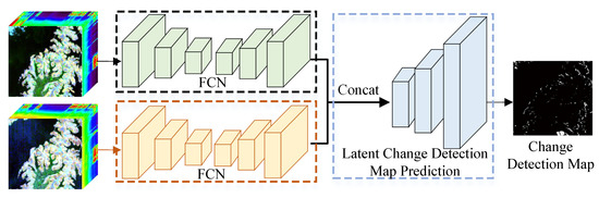
Figure 3.
Architecture of the feature-level fusion.
We perform feature-level fusion with the final layer of the FCN network [52], i.e., and . The reason for this is that the final feature maps are with highest spatial resolution and abstract level. Under this setting, we propose three types of feature fusion method [53]. The first is concatenation. Concatenation is widely used to fuse multiple features, and is effective in many applications. We concatenate the two feature maps along the second axis into one as . Then, is used to generate the change detection map. The second type of fusion strategy is element-wise summation. By adding the two feature maps together, we obtain the final feature maps for the subsequent noise modeling module. Similarly, element-subtraction is also used for the feature fusion. All the aforementioned feature fusion strategies can be formulated as
After the feature fusion module, the fused feature map or is generated, and these feature maps are used for the following noise modeling module to estimate the ‘true’ change detection map.
2.3. Unsupervised Noise Modeling Module
Since ground truth labels can not be used in the HSI change detection task, we propose to make use of the change detection results of existing unsupervised change detection methods to train the FCN network. These samples which are not real labeled data with labor are used to train the network. However, the change detection results of existing unsupervised methods such as CVA [26], PCA-CVA [30], and IR-MAD [34] contain errors, which means that directing training the network with these samples will limit the performance. Inspired by the work of [54], we aim to improve the performance by excluding the noise in the existing change detection maps. Specifically, the noisy but informative change detection maps of existing unsupervised methods are utilized for the training of proposed network.
The two input HSIs are denoted as and , and K existing change detection maps are considered as the training dataset produced by the unsupervised change detection methods. The accuracies of these existing change detection maps are not 100%, which means there are some noises difficult to remove. The output of the proposed FCN-based network is employed to estimate the ‘true’ change detection map. This can be represented as
where is the decoder network. With the two input HSIs, the estimated change map can also be formulated as , where f denotes the whole network. Specifically, to exclude the noise in the training dataset , each pixel in is modeled as the sum of and a Gaussian noise : = + . In practice, given the FCN network parameters and two input HSIs, the noise module can be formulated as
where is a noise map which is subject to a zero-mean Gaussian distribution. The reason why is supposed to be a zero-mean Gaussian distribution is that Gaussian noise may be the best simulation of real noise when the real noise is particularly complex. In addition, the zero-mean Gaussian distribution is very simple and easy to calculate. The distribution of parameter in can be estimated with the following steps during training. Firstly, a noise map is generated from a prior Gaussian distribution . Then, the computed noise map is denoted as
and the corresponding distribution can be estimated with . Finally, the Kullback–Leibler (KL) divergence loss is used to enforce the computed noise map to approximately obey the prior Gaussian distribution . The loss function can be formulated as
With these steps, the noise is separated from the and the change detection performance is improved in an unsupervised manner.
2.4. End-to-End Training
As mentioned above, the proposed FCN-based network firstly learns the latent change detection map, which then is trained to generate the ‘true’ change detection map with the training dataset and the noise modeling module. Since no ground truth labels are used in this work, it is still an unsupervised framework for the change detection task and works in an end-to-end manner. For the change detection map generation, the cross-entropy loss is employed for supervision. Given the predicted change detection map and the training dataset generated from existing unsupervised change detection methods , the cross entropy loss can be computed by
The aforementioned KL divergence loss works natively with the cross entropy loss . Thus, the total loss for the training of the whole framework is denoted as
where the parameter is used to balance the two types of loss functions. In practice, the parameter is set to 0.001. Moreover, in order to make the training process more stable, the FCN network is first trained until it converges. Then, the whole framework is trained with the loss L. The illustration of the training details of the proposed denoising module is depicted in Figure 4.
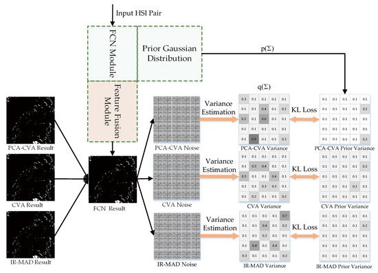
Figure 4.
This figure illustrates the training details of the proposed denoising module. In this module, the latent change detection map generated by the FCN network is subtracted by the unsupervised training datasets to obtain the noise map. Then, we train this module to minimize the Kullback–Leibler (KL) divergence between the noise distribution and the prior Gaussian distribution. Finally, a noise excluded-change detection map is obtained when this module converges.
3. Experiments
In this section, lots of experiments are carried out on three HSI datasets to evaluate the superiority of the proposed method. Firstly, the employed HSI change detection datasets are introduced. Then, we describe the experimental details including evaluation measures and parameter setup. Finally, the experimental results of the proposed method and other state-of-the-art works are analyzed in detail.
3.1. Datasets
In order to evaluate the performance of the proposed method, three HSI change detection datasets are employed, which are from Earth Observing-1 (EO-1) Hyperion hyperspectral sensor. The EO-1 Hyperion sensor offers imagery at 30 meter spatial resolution [55] and the spectral range is from 0.4 to 2.5 m [56]. Additionally, it provides 10 nm spectral resolution and 7.7-km swath width [57]. Each dataset consists of three images, which are HSI of time 1, HSI of time 2, and a ground-truth map. The two real HSIs are photographed at the same place but different times and the corresponding ground-truth map is a binary image. The white pixels in the ground-truth map indicate the changed part while the black pixels mean the unchanged objects. The detailed descriptions of three HSI change detection datasets are shown as follows:
- (1)
- Farmland: This data set covers an area of farmland in the city of Yancheng, Jiangsu province, China, composed of pixels. The two HSIs were taken on 3 May 2006 shown in Figure 5a and 23 April 2007 shown in Figure 5b. After removing the noise and water absorption bands, there are 155 spectral bands used for change detection in the experiments. Additionally, the major change is the size of farmland on this dataset.
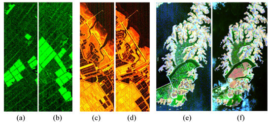 Figure 5. (a) The farmland image on 3 May 2006; (b) The farmland image on 23 April 2007; (c) The countryside image on 3 November 2007; (d) The countryside image on 28 November 2008; (e) The Poyang lake image on 27 July 2002; (f) The Poyang lake image on 16 July 2004.
 - (2)
- Countryside: It covers an area of countryside in the city of Nantong, Jiangsu province, China, shown in Figure 5c,d. The two HSIs were acquired on 3 November 2007 and 28 November 2008, respectively. There are 166 bands used after discarding some noisy bands, and the size of each band is pixels. Visually, the size of rural areas is the main change in this dataset.
- (3)
- Poyang lake: The two HSIs covers the province of Jiangxi, China, obtained on 27 July 2002 and 16 July 2004, respectively. This dataset has a size of and is illustrated in Figure 5e,f. There are 158 spectral bands after noise elimination. In addition, the land change is approximately the major change.
3.2. Experimental Details
3.2.1. Evaluation Measures
Evaluation measures are very important to analyze the performance of change detection methods. In this work, the overall accuracy (OA) and the kappa coefficient are employed to evaluate different change detection methods. In the calculation of OA and kappa coefficient, four indexes are adopted: (1) true positives (TP), the number of changed pixels that are correctly detected; (2) true negatives (TN), the number of unchanged pixels that are correctly detected; (3) the false positives (FP), the number of unchanged pixels that are detected as changed pixels wrongly; (4) the false negatives (FN), the number of changed pixels that are detected as unchanged pixels. Specifically, the OA is defined as
The kappa coefficient is employed as a consistency test, which is an index to evaluate the accuracy of classification. In the change detection task, the kappa coefficient indicates the consistency between the change detection map and the ground-truth map. The larger the value of kappa coefficient, the better the performance of the corresponding method. The kappa coefficient is denoted as
where
3.2.2. Parameter Setup
All of the experiments are conducted on Ubuntu 18.04 with four Nvidia TITAN X Pascal cards. In this work, the change detection is treated as a segmentation task. The training details are introduced as follows. The ImageNet [58] pre-trained parameters are used for the initialization of FCN encoder network. Adam [59] optimizer with decay is employed for the training process. The initial learning is set to for all the three datasets, and no reduction strategy is used during training. For each dataset, we train the whole network with 1200 iterations. For the first 500 iterations, we only train the FCN network. For the remaining 700 iterations, the whole network including the denoising module is trained and updated. In the training of the denoising module, the initial variance of the prior Gaussian distribution is set to 0.1. It is worth mentioning that all the parameters are the same for the three change detection datasets.
The parameter values of other tested methods are as follows: For CVA method, a MATLAB implementation of CVA is used for HSI change detection. In addition, K-means is utilized to output the final change detection map. For the PCA-CVA method, the PCA pre-processing is employed for dimensionality reduction, whose contribution rate is 0.75. Then the CVA method is applied for the PCA outputs. For IR-MAD, we adopt the MATLAB code of Reference [34]. The pseudo-training dataset is used in SVM, which is the same with GETNET. We set C to 2.0 for the SVM classifier, where the linear kernel is used. For the CNN method, a patch-size of 5 is employed to sample pseudo-training patches, and the network backbone is the same with the GETNET but without the affinity matrix. For GETNET, we follow the same parameter settings described in Reference [44].
3.3. Comparison Results
In this section, extensive experiments are conducted to prove the effectiveness of the proposed method. Specifically, we compare it with other change detection methods including unsupervised approaches such as CVA [26], PCA-CVA [30], and IR-MAD [34], and supervised approaches such as support vector machines (SVMs) [60], patch-based CNN and GETNET [44]. The detailed results of the three datasets of seven different methods are presented in Table 2. These methods are divided into ’Pixel based’, ’Patch based’, and ’FCN based’. For each dataset, the proposed method is compared with the other six methods. In addition, the learned change detection maps and the estimated noise maps are further visualized.
Table 2.
The overall accuracy and kappa coefficients of the proposed method and the other six change detection methods for three datasets.
3.3.1. Farmland Dataset
For the farmland dataset, the visualization results of the seven different methods are presented in Figure 6. Specifically, the proposed unsupervised method achieves competitive performance with the supervised method GETNET, and outperforms the other methods. Since the proposed method uses the results of ‘CVA’ and ‘PCA-CVA’, we compare the performance of them with ours. From the results we can see that the proposed denoising module can effectively exclude the noise with the results of ‘CVA’ and ‘PCA-CVA’, and improve the performance in an unsupervised manner. Although GETNET can outperform our method, it employs patch-based CNN network architecture, which is more time-consuming. Since there exists noise in the pseudo-dataset used in SVM and CNN, their performances are lower than the unsupervised CVA, PCA-CVA, and IR-MAD methods. Thus, the noise in the training set can do harm to the accuracy of these methods. However, with the denoising module of the proposed method, our method outperforms the CVA, PCA-CVA, and IR-MAD methods. In addition, the kappa coefficient of the proposed method is also high, indicating that the consistency between our method and the ground-truth map is almost perfect. To sum up, our method is competitive with GETNET and achieves a better performance than the other methods on this dataset.
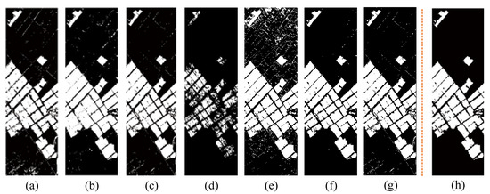
Figure 6.
The change detection maps of different methods for the dataset of farmland, (a) the change detection map of CVA, (b) PCA-CVA, (c) IR-MAD, (d) SVM, (e) CNN (f) GETNET, (g) our method, and (h) ground-truth map.
3.3.2. Countryside Dataset
The countryside dataset is more complicated than the farmland dataset as shown in Figure 7. For this dataset, our method achieves a similar result as with the supervised GETNET method, and outperforms the other methods including the supervised and unsupervised forms. To be specific, the PCA-CVA, IR-MAD, and patch-based CNN methods yield lower OA than that of the farmland dataset since this dataset contains more scatter points and these points make these noise-sensitive methods perform worse. It is worth mentioning that our method achieves a better performance than the patch-based CNN, which is a supervised method with deep learning. This result indicates that the proposed method is robust to noise and excellently improves the performance. Additionally, regarding the kappa coefficient, our method is next only to GETNET. In summary, the proposed framework achieves the second-best OA and is superior to the other five change detection methods.
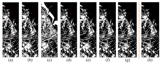
Figure 7.
The change detection maps of different methods on the dataset of countryside: (a) the change detection map of CVA; (b) PCA-CVA; (c) IR-MAD; (d) SVM; (e) CNN; (f) GETNET; (g) our method; and (h) ground-truth map.
3.3.3. Poyang Lake Dataset
The Poyang lake dataset contains more scatter points and is more challenging for pseudo-dataset-based methods. For this dataset, our method works great and is competitive with GETNET. Furthermore, IR-MAD performs worst both on OA and kappa coefficient. What is particularly noteworthy is the proposed method achieves the largest value of kappa coefficient, which means the almost perfect consistency between it and the ground-truth map. Particularly, the performance of our method exceeds the best unsupervised method CVA by about 1%, which indicates the effectiveness of the proposed denoising module. As can be seen in Figure 8g, some of the obvious noise is removed compared to (a), (b), and (c). Although GETNET performs best, it is more complex to train and test. Overall, our method has obvious advantages over the other methods. To better visualize the denoising module, we show the estimated noise map and latent change detection map in Figure 9.
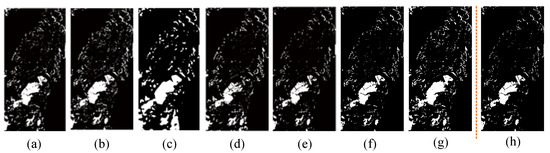
Figure 8.
The change detection maps of different methods for the dataset of Poyang lake: (a) the change detection map of CVA; (b) PCA-CVA; (c) IR-MAD; (d) SVM; (e) CNN; (f) GETNET; (g) our method; and (h) ground-truth map.
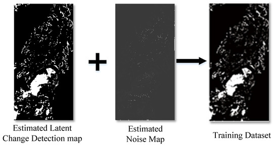
Figure 9.
Illustration of the learned latent change detection map and the estimated noise map. The denoising module separates the training dataset into the latent change detection map and the noise map.
3.3.4. Ablation Study
To evaluate the effect of different feature fusion methods, we conducted several experiments, and the results are shown in Table 3. The results illustrate that feature-level concatenation outperforms other fusion methods. Actually, the element-wise summation and subtraction are special cases regarding the concatenation. When the weights of the next convolution layer are specially structured, the concatenation operation is equal to the summation or subtraction. However, image-level subtraction obtains the worst performance. The reason may be that some important information is lost after the HSI subtraction.
Table 3.
Comparisons of different fusion strategies.
Furthermore, we also conducted experiments to evaluate the effect of the number of unsupervised change detection maps, which are presented in Table 4. The results reveal that using all three unsupervised change detection maps achieves the best performance. Even with only one unsupervised change detection map, our method can still improve the performance compared to the noisy training change detection maps. This indicates the effectiveness of the proposed method.
Table 4.
Comparisons of different number of unsupervised change detection maps.
As for the running time, the proposed framework takes 0.403 s for one inference on the described hardware. However, it takes 139 s for the patch-based method GETNET to generate the final change detection map, which is dramatically slower than the proposed method. Thus, the proposed method is time efficient compared to the patch-based method GETNET.
4. Conclusions
This paper proposes a novel noise modeling-based unsupervised deep FCN framework for HSI change detection. In view of the fact that the high dimension of hyperspectral data has adverse effects on the performance of change detection, an effective deep framework is necessary to deal with this problem. Different from common CNN which learn features with the supervision method, an unsupervised deep FCN framework is presented without any labeled data. It makes use of the results of existing unsupervised change detection methods to train the network in an end-to-end manner. Specifically, the proposed method consists of three main modules, which are the FCN-based feature learning module, the two-stream feature fusion module, and the unsupervised noise modeling module. Firstly, the FCN-based feature learning module is employed to learn discriminative features from bitemporal HSIs. Then, the two-stream feature fusion module fuses the extracted feature for the purpose of the next step. Finally, the unsupervised noise modeling module deals with the influence of noise and is used for the robust training of the proposed network. These three modules work collaboratively towards improving the performance of change detection. A lot of experimental results illustrate that the proposed method is superior to unsupervised methods and some supervised method.
Author Contributions
All authors make contributions to proposing the method, performing the experiments and analyzing the results. All authors contributed to the preparation and revision of the manuscript.
Funding
This research received no external funding.
Acknowledgments
This work was supported by the National Natural Science Foundation of China under Grant U1864204 and 61773316, Natural Science Foundation of Shaanxi Province under Grant 2018KJXX-024, Projects of Special Zone for National Defense Science and Technology Innovation, Fundamental Research Funds for the Central Universities under Grant 3102017AX010, and Open Research Fund of Key Laboratory of Spectral Imaging Technology, Chinese Academy of Sciences.
Conflicts of Interest
The authors declare no conflict of interest.
References
- Kruse, F.A.; Boardman, J.W.; Huntington, J.F. Comparison of Airborne Hyperspectral Data and EO-1 Hyperion for Mineral Mapping. IEEE Trans. Geosci. Remote Sens. 2003, 41, 1388–1400. [Google Scholar] [CrossRef]
- Zhang, L.; Zhang, L.; Tao, D.; Huang, X.; Du, B. Hyperspectral Remote Sensing Image Subpixel Target Detection Based on Supervised Metric Learning. IEEE Trans. Geosci. Remote Sens. 2014, 52, 4955–4965. [Google Scholar] [CrossRef]
- Wang, J.; Zhang, K.; Wang, P.; Madani, K.; Sabourin, C. Unsupervised Band Selection Using Block-Diagonal Sparsity for Hyperspectral Image Classification. IEEE Geosci. Remote Sens. Lett. 2017, 14, 2062–2066. [Google Scholar] [CrossRef]
- Yuan, Y.; Lin, J.; Qi, W. Dual-Clustering-Based Hyperspectral Band Selection by Contextual Analysis. IEEE Trans. Geosci. Remote Sens. 2016, 54, 1431–1445. [Google Scholar] [CrossRef]
- Wang, Q.; Zhang, F.; Li, X. Optimal Clustering Framework for Hyperspectral Band Selection. IEEE Trans. Geosci. Remote Sens. 2018, 56, 5910–5922. [Google Scholar] [CrossRef]
- Yuan, Y.; Ma, D.; Wang, Q. Hyperspectral Anomaly Detection by Graph Pixel Selection. IEEE Trans. Cybern. 2015, 46, 3123–3134. [Google Scholar] [CrossRef] [PubMed]
- Ma, N.; Peng, Y.; Wang, S.; Phw, L. An Unsupervised Deep Hyperspectral Anomaly Detector. Sensors 2018, 18, 693. [Google Scholar] [CrossRef]
- Zhu, L.; Wen, G. Hyperspectral Anomaly Detection via Background Estimation and Adaptive Weighted Sparse Representation. Remote Sens. 2018, 10, 272. [Google Scholar]
- Wang, Q.; Lin, J.; Yuan, Y. Salient Band Selection for Hyperspectral Image Classification via Manifold Ranking. IEEE Trans. Neural Netw. Learn. Syst. 2017, 27, 1279–1289. [Google Scholar] [CrossRef]
- Wang, Q.; He, X.; Li, X. Locality and Structure Regularized Low Rank Representation for Hyperspectral Image Classification. IEEE Trans. Geosci. Remote Sens. 2018. [Google Scholar] [CrossRef]
- Aptoula, E.; Mura, M.D.; Lefèvre, S. Vector Attribute Profiles for Hyperspectral Image Classification. IEEE Trans. Geosci. Remote Sens. 2016, 54, 3208–3220. [Google Scholar] [CrossRef]
- Uezato, T.; Fauvel, M.; Dobigeon, N. Hyperspectral unmixing with spectral variability using adaptive bundles and double sparsity. arXiv, 2018; arXiv:1804.11132. [Google Scholar]
- Aggarwal, H.K.; Majumdar, A. Hyperspectral Unmixing in the Presence of Mixed Noise Using Joint-Sparsity and Total Variation. IEEE J. Sel. Top. Appl. Earth Obs. Remote Sens. 2016, 9, 4257–4266. [Google Scholar] [CrossRef]
- Bioucasdias, J.M.; Plaza, A.; Dobigeon, N.; Parente, M.; Du, Q.; Gader, P.; Chanussot, J. Hyperspectral Unmixing Overview: Geometrical, Statistical, and Sparse Regression-Based Approaches. IEEE J. Sel. Top. Appl. Earth Obs. Remote Sens. 2012, 5, 354–379. [Google Scholar] [CrossRef]
- Li, C.; Liu, Y.; Cheng, J.; Song, R.; Peng, H.; Chen, Q.; Chen, X. Hyperspectral Unmixing with Bandwise Generalized Bilinear Model. Remote Sens. 2018, 10, 1600. [Google Scholar] [CrossRef]
- Eismann, M.T.; Meola, J.; Hardie, R.C. Hyperspectral Change Detection in the Presenceof Diurnal and Seasonal Variations. IEEE Trans. Geosci. Remote Sens. 2008, 46, 237–249. [Google Scholar] [CrossRef]
- Hasanlou, M.; Seydi, S.T. Hyperspectral change detection: An experimental comparative study. Int. J. Remote Sens. 2018, 39, 1–55. [Google Scholar] [CrossRef]
- Seydi, S.T.; Hasanlou, M. Sensitivity analysis of pansharpening in hyperspectral change detection. Appl. Geomat. 2018, 10, 65–75. [Google Scholar] [CrossRef]
- Song, A.; Choi, J.; Han, Y.; Kim, Y. Change Detection in Hyperspectral Images Using Recurrent 3D Fully Convolutional Networks. Remote Sens. 2018, 10, 1827. [Google Scholar] [CrossRef]
- ASHBINDU SINGH. Review Article Digital change detection techniques using remotely-sensed data. Int. J. Remote Sens. 1989, 10, 989–1003. [Google Scholar] [CrossRef]
- Singh, D.; Chamundeeswari, V.V.; Singh, K.; Wiesbeck, W. Monitoring and change detection of natural disaster (like subsidence) using Synthetic Aperture Radar (SAR) data. In Proceedings of the 2008 International Conference on Recent Advances in Microwave Theory and Applications, Jaipur, India, 21–24 November 2008; pp. 419–421. [Google Scholar]
- Kennedy, R.E.; Townsend, P.A.; Gross, J.E.; Cohen, W.B.; Bolstad, P.; Wang, Y.Q.; Adams, P.; Gross, J.E.; Goetz, S.J.; Cihlar, J. Remote sensing change detection tools for natural resource managers: understanding concepts and tradeoffs in the design of landscape monitoring projects. Remote Sens. Environ. 2009, 113, 1382–1396. [Google Scholar] [CrossRef]
- Awad, M. Sea water chlorophyll-a estimation using hyperspectral images and supervised Artificial Neural Network. Ecol. Inform. 2014, 24, 60–68. [Google Scholar] [CrossRef]
- Lunetta, R.S.; Knight, J.F.; Ediriwickrema, J.; Lyon, J.G.; Worthy, L.D. Land-cover change detection using multi-temporal MODIS NDVI data. Remote Sens. Environ. 2009, 105, 142–154. [Google Scholar] [CrossRef]
- Hégarat-Mascle, S.L.; Ottlé, C.; Guérin, C. Land cover change detection at coarse spatial scales based on iterative estimation and previous state information. Remote Sens. Environ. 2018, 95, 464–479. [Google Scholar]
- Malila, W.A. Change Vector Analysis: An Approach for Detecting Forest Changes with Landsat. 1980. Available online: https://docs.lib.purdue.edu/lars_symp/385/ (accessed on 1 January 2018).
- Bovolo, F.; Marchesi, S.; Bruzzone, L. A Framework for Automatic and Unsupervised Detection of Multiple Changes in Multitemporal Images. IEEE Trans. Geosci. Remote Sens. 2012, 50, 2196–2212. [Google Scholar] [CrossRef]
- Bovolo, F.; Bruzzone, L. A Theoretical Framework for Unsupervised Change Detection Based on Change Vector Analysis in the Polar Domain. IEEE Trans. Geosci. Remote Sens. 2006, 45, 218–236. [Google Scholar] [CrossRef]
- Bovolo, F.; Bruzzone, L. An adaptive thresholding approach to multiple-change detection in multispectral images. In Proceedings of the 2011 IEEE International Geoscience and Remote Sensing Symposium, Vancouver, BC, Canada, 24–29 July 2011; Volume 4, pp. 233–236. [Google Scholar]
- Baisantry, M.; Negi, D.S.; Manocha, O.P. Change Vector Analysis using Enhanced PCA and Inverse Triangular Function-based Thresholding. Defence Sci. J. 2012, 62, 236–242. [Google Scholar] [CrossRef]
- Zhuang, H.; Deng, K.; Fan, H.; Yu, M. Strategies Combining Spectral Angle Mapper and Change Vector Analysis to Unsupervised Change Detection in Multispectral Images. IEEE Geosci. Remote Sens. Lett. 2017, 13, 681–685. [Google Scholar] [CrossRef]
- Thonfeld, F.; Feilhauer, H.; Braun, M.; Menz, G. Robust Change Vector Analysis (RCVA) for multi-sensor very high resolution optical satellite data. Int. J. Appl. Earth Obs. Geoinform. 2016, 50, 131–140. [Google Scholar] [CrossRef]
- Nielsen, A.A.; Conradsen, K.; Simpson, J.J. Multivariate Alteration Detection (MAD) and MAF Postprocessing in Multispectral, Bitemporal Image Data: New Approaches to Change Detection Studies. Remote Sens. Environ. 1998, 64, 1–19. [Google Scholar] [CrossRef]
- Nielsen, A.A. The regularized iteratively reweighted MAD method for change detection in multi- and hyperspectral data. IEEE Trans. Image Process. A Publ. IEEE Signal Process. Soc. 2007, 16, 463–478. [Google Scholar] [CrossRef]
- Liu, S.; Du, Q.; Tong, X.; Samat, A.; Pan, H.; Ma, X.; Liu, S.; Du, Q.; Tong, X.; Samat, A. Band Selection-Based Dimensionality Reduction for Change Detection in Multi-Temporal Hyperspectral Images. Remote Sens. 2017, 9, 1008. [Google Scholar] [CrossRef]
- Shao, P.; Shi, W.; He, P.; Hao, M.; Zhang, X. Novel Approach to Unsupervised Change Detection Based on a Robust Semi-Supervised FCM Clustering Algorithm. Remote Sens. 2016, 8, 264. [Google Scholar] [CrossRef]
- Zhou, J.; Kwan, C.; Ayhan, B.; Eismann, M.T. A Novel Cluster Kernel RX Algorithm for Anomaly and Change Detection Using Hyperspectral Images. IEEE Trans. Geosci. Remote Sens. 2016, 54, 6497–6504. [Google Scholar] [CrossRef]
- Erturk, A.; Iordache, M.D.; Plaza, A. Sparse Unmixing-Based Change Detection for Multitemporal Hyperspectral Images. IEEE J. Sel. Top. Appl. Earth Obs. Remote Sens. 2017, 9, 708–719. [Google Scholar] [CrossRef]
- Yuan, Y.; Lv, H.; Lu, X. Semi-supervised change detection method for multi-temporal hyperspectral images. Neurocomputing 2015, 148, 363–375. [Google Scholar] [CrossRef]
- Adão, T.; Hruška, J.; Pádua, L.; Bessa, J.; Peres, E.; Morais, R.; Sousa, J.J. Hyperspectral Imaging: A Review on UAV-Based Sensors, Data Processing and Applications for Agriculture and Forestry. Remote Sens. 2017, 9, 1110. [Google Scholar] [CrossRef]
- Jakovels, D.; Filipovs, J.; Erins, G.; Taskovs, J. Airborne hyperspectral imaging in the visible-to-mid wave infrared spectral range by fusing three spectral sensors. In Proceedings of the Earth Resources and Environmental Remote Sensing/GIS Applications V; SPIE: Bellingham, WA, USA, 2014. [Google Scholar]
- Krizhevsky, A.; Sutskever, I.; Hinton, G.E. ImageNet Classification with Deep Convolutional Neural Networks. In Proceedings of the International Conference on Neural Information Processing Systems, Lake Tahoe, Nevada, 3–6 December 2012; pp. 1097–1105. [Google Scholar]
- He, K.; Zhang, X.; Ren, S.; Sun, J. Deep Residual Learning for Image Recognition. In Proceedings of the IEEE Conference on Computer Vision and Pattern Recognition, Las Vegas, NV, USA, 27–30 June 2016; pp. 770–778. [Google Scholar]
- Wang, Q.; Yuan, Z.; Du, Q.; Li, X. GETNET: A General End-to-end Two-dimensional CNN Framework for Hyperspectral Image Change Detection. IEEE Trans. Geosci. Remote Sens. 2019, 57, 3–13. [Google Scholar] [CrossRef]
- Zhao, W.; Wang, Z.; Gong, M.; Liu, J. Discriminative Feature Learning for Unsupervised Change Detection in Heterogeneous Images Based on a Coupled Neural Network. IEEE Trans. Geosci. Remote Sens. 2017, 55, 1–15. [Google Scholar] [CrossRef]
- Amin, A.M.E.; Liu, Q.; Wang, Y. Zoom out CNNs features for optical remote sensing change detection. In Proceedings of the International Conference on Image, Vision and Computing, Chengdu, China, 2–4 June 2017; pp. 812–817. [Google Scholar]
- de Jong, K.L.; Bosman, A.S. Unsupervised Change Detection in Satellite Images Using Convolutional Neural Networks. arXiv, 2018; arXiv:1812.05815. [Google Scholar]
- Mandić, I.; Peić, H.; Lerga, J.; Štajduhar, I. Denoising of X-ray Images Using the Adaptive Algorithm Based on the LPA-RICI Algorithm. J. Imaging 2018, 4, 34. [Google Scholar] [CrossRef]
- Wang, Q.; Wan, J.; Nie, F.; Liu, B.; Yan, C.; Li, X. Hierarchical feature selection for random projection. IEEE Trans. Neural Netw. Learn. Syst. 2018. [Google Scholar] [CrossRef]
- Wang, Q.; Chen, M.; Nie, F.; Li, X. Detecting coherent groups in crowd scenes by multiview clustering. IEEE Trans. Pattern Anal. Mach. Intell. 2018. [Google Scholar] [CrossRef] [PubMed]
- Lee, S.; Park, S.J.; Hong, K.S. RDFNet: RGB-D Multi-level Residual Feature Fusion for Indoor Semantic Segmentation. In Proceedings of the IEEE International Conference on Computer Vision, Venice, Italy, 22–29 October 2017. [Google Scholar]
- Shelhamer, E.; Long, J.; Darrell, T. Fully Convolutional Networks for Semantic Segmentation. In Proceedings of the 2015 IEEE Conference on Computer Vision and Pattern Recognition (CVPR), Boston, MA, USA, 7–12 June 2015; Volume 39, pp. 640–651. [Google Scholar]
- Li, Y.; Zhang, J.; Cheng, Y.; Huang, K.; Tan, T. DF2Net: Discriminative Feature Learning and Fusion Network for RGB-D Indoor Scene Classification. In Proceedings of the Thirty-Second AAAI Conference on Artificial Intelligence, New Orleans, LA, USA, 2–7 February 2018; pp. 7041–7048. [Google Scholar]
- Zhang, J.; Zhang, T.; Dai, Y.; Harandi, M.; Hartley, R.I. Deep Unsupervised Saliency Detection: A Multiple Noisy Labeling Perspective. In Proceedings of the 2018 IEEE Conference on Computer Vision and Pattern Recognition, CVPR 2018, Salt Lake City, UT, USA, 18–22 June 2018; pp. 9029–9038. [Google Scholar]
- Folkman, M.A.; Jarecke, P.J. EO-1/Hyperion hyperspectral imager design, development, characterization, and calibration. Hyperspectral Remote Sens. Land Atmos. 2001, 4151, 40–51. [Google Scholar]
- Datt, B.; Mcvicar, T.R.; Van Niel, T.G.; Jupp, D.L.B.; Pearlman, J.S. Preprocessing EO-1 Hyperion hyperspectral data to support the application of agricultural indexes. IEEE Trans. Geosci. Remote Sens. 2003, 41, 1246–1259. [Google Scholar] [CrossRef]
- Pearlman, J.S.; Barry, P.S.; Segal, C.C.; Shepanski, J.; Beiso, D.; Carman, S.L. Hyperion, a Space-Based Imaging Spectrometer. IEEE Trans. Geosci. Remote Sens. 2003, 41, 1160–1173. [Google Scholar] [CrossRef]
- Deng, J.; Dong, W.; Socher, R.; Li, L.J.; Li, K.; Fei-Fei, L. ImageNet: A large-scale hierarchical image database. In Proceedings of the IEEE Conference on Computer Vision and Pattern Recognition, 2009 (CVPR 2009), Miami, FL, USA, 20–25 June 2009; pp. 248–255. [Google Scholar]
- Kingma, D.P.; Ba, J. Adam: A method for stochastic optimization. arXiv, 2014; arXiv:1412.6980. [Google Scholar]
- Nemmour, H.; Chibani, Y. Multiple support vector machines for land cover change detection: An application for mapping urban extensions. Isprs J. Photogramm. Remote Sens. 2006, 61, 125–133. [Google Scholar] [CrossRef]


© 2019 by the authors. Licensee MDPI, Basel, Switzerland. This article is an open access article distributed under the terms and conditions of the Creative Commons Attribution (CC BY) license (http://creativecommons.org/licenses/by/4.0/).