Article

Deriving a Forest Cover Map in Kyrgyzstan Using a Hybrid Fusion Strategy

1
School of Remote Sensing and Information Engineering, Wuhan University, Wuhan 430072, China
2
Department of Land Surveying and Geo-informatics, The Hong Kong Polytechnic University, Kowloon 999077, Hong Kong, China
3
School of Geomatics and Urban Spatial Information, Beijing University of Civil Engineering and Architecture, Beijing 100044, China
*
Author to whom correspondence should be addressed.
Remote Sens. 2019, 11(19), 2325; https://doi.org/10.3390/rs11192325
Submission received: 22 July 2019 / Revised: 29 September 2019 / Accepted: 3 October 2019 / Published: 6 October 2019
(This article belongs to the Section Forest Remote Sensing)

Abstract

:
Forests have potential economic value and play a significant role in maintaining ecological balance. Considering its outdated and incomplete forest statistics, the Kyrgyzstan Republic urgently needs a forest cover map for assessing its current forest resources and assisting national policies on improving rural livelihood and sustainability. This study adopted a hybrid fusion strategy to develop a forest cover map for the Kyrgyzstan Republic with improved accuracy. The fusion strategy uses the merits of the GlobeLand30 in 2010 and the USGS TreeCover2010, the benefits of auxiliary geographic information, and the advantages of the stacking learning method in classification. Additionally, we explored the influence of different forest definitions, based on the tree cover percentage value in the USGS TreeCover2010, on the accuracy of forest cover. Results suggested that the accuracy of our model can be improved significantly by including auxiliary geographic features and feeding the optimal size of training samples. Thereafter, using our model, forest cover maps were derived at different tree cover threshold values in the USGS TreeCover2010. Importantly, the forest cover map at the tree cover threshold value of 40% was determined as the most accurate one with the kappa value of 0.89, whose spatial extent constitutes about 2.4% of the entire territory. This estimated forest cover percentage suggests a low estimation of forest resources based on rigorous definition, which can be valuable for reviewing and amending the current national forest policies.

Graphical Abstract

1. Introduction

Forest is an important natural resource that provides numerous benefits for many fields including economy, society, and environment. It not only serves as a source of timber or an area for recreational activities, but also plays a significant role in maintaining ecological balance, such as converting carbon dioxide into oxygen and biomass, mitigating natural hazards, and regulating climate or water [1,2]. It is reported that the amount of forest in the world continues to decrease due to the growth of population and the conversion of forest land into agricultural land or others, although the rate of net global deforestation has slowed down in the past 25 years [3]. Specifically, deforestation in the Kyrgyzstan Republic might have a significant influence on both regional hydrology [4] and livelihoods of rural communities accounting for two-thirds of the total population. Besides, the Kyrgyzstan Republic is transiting from a planned economy to a market economy, which suggests the importance of understanding the economic value and potential of forest resources. In this context, it urgently needs a forest cover map for assessing its existing forest resources and assisting national policies on improving rural livelihood and managing forest resources productively in a sustainable manner. However, forest statistics in the Kyrgyzstan Republic are outdated or missing after the collapse of the Soviet Union, and only 60% of government-owned forests were inventoried in a recent national survey in 2005. Furthermore, the Food and Agriculture Organization of the United Nations (FAO) might have overestimated the forest cover percentage as 5% in 2010 according to its country report [4]. Hence, a complete picture of forest cover is unclear [2].
Recent development of remote sensing technologies can provide seamless and periodic observations for countries or regions with inconsistent forest statistics [5,6]. The remote sensing data have become a primary data source for deriving spatial distribution of forest cover [7,8], which is of fundamental importance for understanding their current status and thereafter achieving a sustainable forest management [9]. However, the consistency of spectral response across space might be compromised by the complexity of both environment and forest characteristics [10], and it is not a trivial task to derive a forest cover map with high accuracy. On one hand, researchers argued that the specific class mapping outperformed the multi-class supervised classification, and the strategy is to decompose the multi-class task into a series of binary classification tasks for a higher overall accuracy [11,12,13]. For instance, Silva et al. [14] adopted the weighted support vector machines classifier to map two types of mangrove forest using Landsat Thematic Mapper (TM) data. On the other hand, it is widely recognized that a group of classification methods can be fused to achieve higher accuracy than a single classification method [10,15], and the fusion strategy can be “bagging” with a simple combination rule or “stacking” using a meta-classification model. For instance, Clinton et al. [15] proposed geographic stacking methods to enhance the accuracy of a land cover map by up to 6.6% in California.
The previous studies can improve the mapping accuracy, but it is still time-consuming and labor-intensive work to derive an accurate map nationally or globally, because a huge amount of training samples need to be manually selected and labeled considering the uneven distribution of forest across space. Recently, it has been facilitated by the free availability of regional or global land cover products, which were developed using different datasets and different methodologies [16,17]. The regional land cover maps, such as the North America Forest Disturbance product [18] or the Russia forest cover map [19], can provide sufficient spatial and thematic details, but very few of them cover the countries in Central Asia. In addition, the global land cover products vary in spatial resolutions. The coarse resolution products can provide forest cover data, such as GLC2000 at 1000 m with forest cover percentage of 13.5% [20] or MODIS at 500 m with percentage of 0.54% [21], but they cannot satisfy the forest mapping in terms of forest planning and ecological governance at a national scale [22]. On the other hand, the fine resolution maps at 30 m, such as the USGS TreeCover2010 [23] and the GlobeLand30 [24], might be potential data sources. Nonetheless, they are reported to have different accuracies for the forest in the same region [24,25]. For instance, the user’s accuracies of forest in the GlobeLand30 and TreeCover2010 are 0.84 and 0.94 for the Loess Plateau, China in 2010, respectively [25]. Thus, a combination of the two fine resolution products not only gives a reliable and cost-effective way to carry out the selection of massive training samples, but also indicates a potential way for deriving a forest cover map with improved accuracy.
The main objective of this study is to develop a forest cover map with improved accuracy at the resolution of 30 m for the Kyrgyzstan Republic. To achieve this objective, a hybrid fusion strategy is adopted, which includes land cover product fusion, geographical feature fusion, and classifier fusion. First, the GlobeLand30 product and the USGS TreeCover2010 are fused to integrate their advantages on forest definitions. Second, multiple geographical datasets are utilized to supply auxiliary geographic information. Third, a two-layer structured classification system is proposed by fusing multiple classifiers in a hierarchical way. Importantly, previous studies simply extracted forest cover map from the USGS TreeCover2010 by specifying a certain tree cover percentage value [26], but we explored the influence of different tree cover threshold values on generating the forest cover map. Therefore, contributions of this study include: (1) we proposed a cost-effective and reliable framework to map the forest cover with improved accuracy using a hybrid fusion strategy, which can be also used to other countries or other types of land covers; (2) we explored the influence of different forest definitions on the accuracy of forest cover, which could help to improve the accuracy of forest cover map for the Kyrgyzstan Republic.

2. The Study Area and Its Geographical Datasets
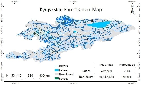
2.1. The Study Area

The Kyrgyzstan Republic is located in Central Asia, which is a landlocked country surrounded by Kazakhstan, Uzbekistan, Tajikistan, and China, as shown in Figure 1a. Around 80% of its territory is occupied by mountainous regions. Forests are relatively scarce in this country, and most of them are distributed around the regions with altitude ranging from 700 meters to 3600 meters; however, they play a significant role in the environment, society, and economy. The Kyrgyzstan Republic’s forests are very important for the diversity of local biological systems, which are homes of many endemic trees including the largest remaining wild forest of walnut in the world. As for society, around 65% of population live in rural mountainous regions relying on livestock and farming, where forests can maintain water balance to ensure the quality and amount of water required by the rural communities upstream and downstream. Importantly, recent policies have realized the utilization of forests for timber, grazing animals, beekeeping, and collecting fruits or nuts, and they also recognized the crucial role of forests in the economy of both local rural communities and the entire country. However, existing forest inventories are incomplete and outdated, and a high accuracy forest cover map is highly required for sustainable development of the environment, society, and economy. Therefore, the entire Kyrgyzstan Republic is selected as the study area.

2.2. The Geographical Datasets and Their Preprocessing

2.2.1. The GlobeLand30 Product

The GlobeLand30 product in 2010 can be freely available from the official site of National Geomatics Center of China, which is composed of 853 data tiles all over the world. It is the result of a four-year project in China aiming to produce a global land cover dataset at the spatial resolution of 30 m [27]. It was developed using more than 10,000 satellite images. A total number of 10 land cover types were identified and mapped, where forest cover was the focus of this study [24]. Accuracy assessment results suggested that the user’s accuracy of forest cover was 0.83, but the producer’s accuracy was missing. Hence, it is still an open question on forest accuracy around the world or particularly in the Kyrgyzstan Republic [25]. In this study, this dataset was preprocessed with three steps. The first step was to mosaic the data titles to produce a raster map covering the entire country, the second step was to re-project the map into the Universal Transverse Mercator (UTM) coordinate system, and the last step was to clip the projected map with boundaries of the Kyrgyzstan Republic. All these steps were carried out in ArcGIS. As shown in Figure 1b, forest cover was extracted simply by identifying the pixels labeled as forests and directly used in our method in Section 3. Additionally, a simple statistical analysis suggested that the estimated forest area is about 1,556,390 ha and constitutes around 7.8% of the entire territory, which is relatively larger than the amount of 954,000 ha summarized by FAO in 2010 [28].

2.2.2. The USGS TreeCover2010 Dataset

The USGS TreeCover2010 product can be freely downloaded from the official site of the Global Land Analysis and Discovery (GLAD) laboratory at the University of Maryland, which is organized in data tiles of 10 × 10 degrees from 80° north to 60° south. It is a global tree cover map produced through a collaboration between the USGS and the University of Maryland, which was derived from cloud-free annual growing season composite Landsat TM/ETM+ images and global MODIS Vegetation Continuous Fields (VCF) products. In this map, tree cover canopy is defined as horizontal ground covered by woody vegetation greater than 5 meters in height. It contains per pixel estimates (1–100%) of percent maximum tree canopy cover at the spatial resolution of 30 m for the year 2010 [23]. Accuracy assessment results suggested that user’s accuracy and producer’s accuracy for forest loss detection are greater than 80% and the overall accuracy for both forest gain and forest loss exceeds 90% at the global extent [23]. This dataset is preprocessed using the same steps as the GlobeLand30 product in ArcGIS, and, as shown in Figure 1c, tree cover percentage was visualized and used directly in our method in Section 3.
Owing to its definition, forest cover in the USGS TreeCover2010 can be extracted at different tree cover threshold values. As shown in Table 1, we compared forest cover in the USGS TreeCover2010 at different tree cover threshold values with forest cover in the GlobeLand30 product. As the tree cover threshold value increases from 10% to 90%, forest cover area estimated by the USGS TreeCover2010 decreases dramatically from 89.61 (104 ha) to 100 ha, which corresponds to a reduction of forest cover percentage from 4.48% to 0.0004%. At the same time, forest difference from the GlobeLand30 becomes larger and larger, which gives rise to the question of how to determine the optimal tree cover threshold value for a better fusion with the forest in the GlobeLand30.

2.2.3. Landsat Images

Landsat-5 TM images can be freely downloaded from the USGS archives at the spatial resolution of 30 m, which record digital information of the reflected and emitted energy from Earth in various wavelengths of the electromagnetic spectrum. Each image has 7 bands, but only 6 bands were used in our study except for the thermal band. It should be noted that only images with low cloud coverage were chosen during the growing season in 2010. Thereafter, a total number of 26 Landsat-5 TM images (including 156 bands) covering the entire country were adopted in this study. These images were then preprocessed with four steps. The first step was to correct for the effects of clouds and aerosols using the Quick Atmospheric Correction model in ENVI, which is a reliable and fast method without ancillary information to derive apparent surface reflectance images. The second step was to mosaic the 26 TM images with respect to each band in ArcGIS, which was intended to produce a seamless large image covering the entire country. The third step was to re-project the mosaicked images into the UTM coordinate system in ArcGIS. The fourth step was to clip the projected images with the boundary of the Kyrgyzstan Republic in ArcGIS, which produced an input image of 6 bands for our method. As shown in Figure 1d, we visualized band 4, 3, 2 of the input image with the color of red, green, and blue, where vegetation appeared red. In this study, the input image of 6 bands was mainly used to derive the normalized difference vegetation index (NDVI) map and to reveal the characteristics of spectral features and texture features to distinguish forest cover from non-forest cover, which is elaborated in detail in Section 3.

2.2.4. The Ancillary Geographical Datasets

The auxiliary geographical datasets include the digital elevation model (DEM) and the MODIS land surface temperature (LST) product MOD11A2 [29]. DEM was produced by NASA under the shuttle radar topographic mission [30], which is now freely available under its fourth version and known as the highest quality elevation data for the whole world at the spatial resolution of 90 m. Its vertical error is reported to be less than 16 m, and there are very few no-data regions in our study area. MOD11A2 was produced by the NASA MODIS land team in 2010 and is freely available for the globe at the spatial resolution of 1 km. In this study, we used the MOD11A2 product in May 2010, where each pixel records the 8-day average value of clear-sky land surface temperature. The two datasets were then preprocessed with four steps. The first step was to re-sample the two datasets such that they had the same spatial resolution of 30 m, the second step was to mosaic each dataset such that it covered the entire country, the third step was to re-project the two datasets into the UTM coordinate system, and the last step was to clip each dataset using the boundary of the Kyrgyzstan Republic. It should be noted that the four steps were carried out in ArcGIS. As shown in Figure 1e,f, DEM and land surface temperature of the Kyrgyzstan Republic are displayed. These datasets can benefit forest classification by providing auxiliary geographic information (e.g. temperature tends to be more moderate in forest cover area) and improving classification accuracy, which is elaborated in detail in Section 3.

3. Methodologies

3.1. Land Cover Product Fusion

As shown in Figure 2, the first stage was the fusion of forest cover in the GlobeLand30 product and forest cover in the USGS TreeCover2010 map at tree cover threshold value α, which aimed to demarcate the study area into the consistent area and the conflicting area. The consistent area was composed of pixels that were labeled as forest or non-forest by both of the two products, e.g. a pixel with value of 1 in the two images was considered as a consistent forest pixel. The conflicting area consisted of pixels that were labeled as different land cover types, e.g. a pixel with value of 1 in the GlobeLand30 and value of 0 in the USGS TreeCover2010 was regarded as a conflicting pixel. The combination fully utilized the advantages of the existing two products on their agreements on definitions of forest and non-forest, which might have reduced the uncertainty of forest mapping. In addition, the consistent area provided a cost-effective way to generate training samples automatically for our classification system, and the conflicting area was left for prediction.

3.2. Geographical Feature Fusion

The second stage of fusion intended to characterize forest and non-forest by extracting geographical features from the datasets of TM images, digital elevation model, and land surface temperature map. Thus, for a given pixel, its feature vector could be extracted from the multiple datasets. Basically, the preprocessed TM image included six bands, which were used to extract three spectral features and three texture features. Spectral features could be denoted as the three largest principal components of the six bands from a Principal Components Analysis (PCA). Texture information of one band could be calculated as four second-order metrics using the window size of 5 × 5 pixels, which included neighborhood entropy, local homogeneity (inverse difference moment), local energy (angular second moment), and local variance [31]. Thus, texture information of six bands could be represented as 24 texture bands, and texture features could be denoted as the three largest principal components of 24 texture bands using a PCA technique. Additionally, two extra features were incorporated, including the NDVI value calculated from the TM image, and the texture feature determined as the largest principal component from a PCA on a four texture band of NDVI. Furthermore, four extra features were added, which included height, aspect, and slope calculated from a terrain analysis on DEM and temperature extracted from a land surface temperature map. It was our assumption that feature fusion with auxiliary geographic information could better characterize forest and non-forest, and hence improve the accuracy of forest cover mapping, which is discussed in Section 5. Therefore, in our method, the twelve-dimensional feature vector including auxiliary geographic information was adopted for the classification.

3.3. Classifier Fusion

The third stage was the fusion of multiple classifiers in a stacking manner, which is a two-layer structured classification system. The first layer contained five base classifiers, and the second layer included one best meta-classifier. Importantly, the five base classifiers were selected such that they were different from each other in terms of classification mechanisms, parameter settings, and the degree of randomization, and the meta-classifier was selected from two potential ones such that it had the highest accuracy and could improve the accuracy over any base classifiers [15].

3.3.1. Preliminaries on Classifiers

A classifier is used to predict the class label from a given feature vector, and it can be formulated as y ^ = C ( x ) , where x is the feature vector, y ^ is the class label predicted by the classifier, and C is the classifier inferred from the training data containing a set of feature vectors (x) together with their class labels (e.g. forest or non-forest). Besides, many metrics are proposed to assess the accuracy of the classifier, such as overall accuracy, producer’s accuracy, and user’s accuracy. However, given the imbalanced training data (a majority of non-forest versus a minority of forest), we adopted the metrics of kappa statistic, F1 score, and G statistic [32].
Kappa statistic measures how well the classification performs as compared to a completely random classification, G statistic is defined as the geometric mean of producer’s accuracy on forest and non-forest, and F1 score is the harmonic mean of producer’s accuracy on forest and user’s accuracy on forest.
K a p p a = | T | ( x { T f } I ( C ( x ) = l f ) + x { T n f } I ( C ( x ) = l n f ) ) ( | T f | x { T } I ( C ( x ) = l f ) + | T n f | x { T } I ( C ( x ) = l n f ) ) | T | | T | ( | T f | x { T } I ( C ( x ) = l f ) + | T n f | x { T } I ( C ( x ) = l n f ) )
G = 1 | T f | x { T f } I ( C ( x ) = l f ) 1 | T n f | x { T n f } I ( C ( x ) = l n f )
F 1 s c o r e = 2 ( x { T f } I ( C ( x ) = l f ) / | T f | ) ( x { T f } I ( C ( x ) = l f ) / x { T } I ( C ( x ) = l f ) ) ( x { T f } I ( C ( x ) = l f ) / | T f | ) + ( x { T f } I ( C ( x ) = l f ) / x { T } I ( C ( x ) = l f ) )
where {T} is the set of test data, |T| is the size of test data, {Tf} is the set of forest test data with class label lf, |Tf| is the size of forest test data, {Tnf} is the set of non-forest test data with class label lnf, |Tnf| is the size of non-forest test data, and I(●) is the indicator function.

3.3.2. Base Classifier

Five different base classifiers were adopted, which included K-nearest neighbor (KNN), multi-layer perceptron (MLP), random forest (RF), extra-trees (EXT), and decision tree based bagging (DTB). These base classifiers are widely used in remote sensing images and have different kinds of expertise in classification. According to classification mechanism, they can be categorized into three groups, where the first group includes the non-parametric classifier KNN, the second group includes the neural network based classifier MLP, and the third group contains the parametric tree-based classifiers in terms of RF, EXT, and DTB. Besides, differences among the classifiers in the third group can be further distinguished from the aspects of parameter settings and randomization. Parameter settings are mainly related to organization of training samples and usage of feature space, while randomization refers to the degree to which the split is determined in random during the construction of a tree classifier. The different classification mechanisms, different parameter settings, and different degrees of randomization could capture distinct feature patterns, which could lead to different prediction results and further add to the diversity of the stacking classification system.
Specifically, the KNN classifier is a lazy classifier that assigns the most frequent class label among the k nearest training samples to the predicted pixel, where the value of k is set as 10 according to the experimental performance. The MLP classifier is a non-linear artificial neural network classifier that uses backpropagation to train a multilayer perceptron by minimizing the amount of error in the output compared to the expected result, where two hidden layers with the sizes of 80 and 10 are adopted based on parameters adjustment. The RF, EXT, and DTB classifiers are all built from a set of trees and make prediction by averaging predictions from individual tree classifiers, but they differ remarkably in parameter settings and randomization. As for the DTB classifier, each tree classifier is trained on random sample drawn from the training set, and all the features are used to determine the best split value without randomness. As for the RF classifier, each tree classifier is also trained on the random set drawn from the training set, but it uses random subsets of features to determine the most discriminative splitting value. This randomness might increase the bias but can be compensated by the decrement of variance owing to averaging. Different from the RF classifier, each tree classifier in EXT is trained using the entire training data, but a further step of randomization is adopted to choose the splitting value instead of the most discriminative one, which might both increase the bias and reduce the variance a bit more [13].

3.3.3. Meta-Classifier

A meta-classifier is trained with the predictions of base classifiers and makes predictions based on the predicted features. However, meta-classifiers differ in their capacities to make accurate predictions, and thus two meta-classifiers were examined in our study, which include logistic regression (LR) and gradient boosting machines (GBM). LR is a consistent and simple method to learn how to combine the predictions from base classifiers and is well suited to this binary classification problem as it produces binary outputs itself. GBM aims to optimize the loss function by adding weak learners and applying a gradient boosting method, which also supports the binary classification problem very well. As a rule of thumb, the meta-classifier should be determined as the one that has a higher accuracy and outperforms all base classifiers. Therefore, in this method, GBM was adopted as the meta-classifier in our classification system, because it showed a relatively higher accuracy than the alternative LR and outperformed the five base classifiers, which is discussed in Section 5.

3.3.4. The Two-Layer Structured Classification System

As aforementioned, the two-layer structured classification system is composed of five base classifiers and one meta-classifier. This classification system belongs to the family of ensemble methods, which is believed to be superior to the other two types of ensemble methods, such as bagging and boosting, in most cases [33]. It should be noted that classifiers in our classification system were implemented using the Scikit-learn open source machine learning package [34], and that parameters included in our classifiers were not tuned except as noted. Firstly, samples of forest and non-forest were randomly selected from the consistent area (α) to train and validate individual base classifiers, for instance, y ^ i b a s e = C i b a s e ( x ) , where y ^ i b a s e was the class label predicted by the ith base classifier C i b a s e . Secondly, predictions from the five base classifiers were organized as a feature vector to train and validate the meta-classifier, for instance, y ^ m e t a = C m e t a ( y ^ K N N b a s e , y ^ E X T b a s e , y ^ R F b a s e , y ^ M L P b a s e , y ^ D T B b a s e ) , where y ^ m e t a was the class label predicted by the meta-classifier C m e t a or the final output of our classification system. Thirdly, the predicted results (forest and non-forest) from the conflicting area were merged with the consistent area to obtain the forest cover map at certain tree cover threshold value. However, it was not a trivial task to determine the optimal sample size, and we solved it by gradually increasing the sample size to detect the optimal one giving improved accuracy. Therefore, in this study, the optimal sample sizes of forests were determined as 70,000, 80,000, 110,000, 100,000, 100,000, and 110,000 at tree cover threshold values of 10%, 20%, 30%, 40%, 50%, and 60%, respectively, which is discussed in Section 5.

3.4. Selection of Optimal α to Derive Forest Cover Map with High Accuracy

The last stage was to select the optimal tree cover threshold value α such that a high accurate forest cover map could be developed. On one hand, a large value of tree cover threshold α can result in the consistent area with small extent, which could strengthen the reliability of forest samples and consequently improve the accuracy of our classification system. However, it cannot guarantee a high accurate forest cover map due to the large number of pixels to be estimated in the conflicting area, which will introduce uncertainties to our final forest cover map. On the other hand, a small value of tree cover threshold α can result in the consistent area with large extent, which could lead to the unreliability of forest samples and consequently decrease the accuracy of our classification system, although the number of pixels to be estimated in the conflicting area is relatively small. Hence, it is not a trivial task to determine the optimal tree cover threshold value α. To examine this issue, a number of test samples were uniformly selected from the entire study area to evaluate the accuracy of forest cover map at certain tree cover threshold value α. Specifically, a total number of 1,898 forest samples and 8,025 non-forest samples were identified by visual interpretation from Google Earth images in the same time period. Using these testing samples, accuracy in terms of kappa, G, and F1 score were calculated for each forest cover map at tree cover threshold value α, and a high accuracy forest cover map was derived at the optimal tree cover threshold value α giving the highest accuracy.

4. Results

Using our classification system, we derived forest cover products at tree cover threshold values of 10%, 20%, 30%, 40%, 50%, and 60%. As shown in Figure 3a, a combination of the USGS TreeCover2010 at tree cover threshold value of 40% and the GlobeLand30 could produce a forest cover map with kappa value of 0.89, G value of 0.86, and F1 score value of 0.91, which was the most accurate one among the products at different tree cover threshold values. For instance, kappa values of the forest cover product at tree cover threshold value of 40% were approximately 5.4%, 2.3%, 1.5%, 6.9%, and 14.4% higher than those of forest cover products at tree cover threshold values of 10%, 20%, 30%, 50%, and 60%, respectively. As shown in Figure 3b,c, similar finding could be also reported for G value and F1 score.
Besides, our forest cover products at different tree cover threshold values were compared with the GlobeLand30 and the USGS TreeCover2010. As shown in Figure 3a, kappa values of our forest cover products at tree cover threshold values of 10%, 20%, 30%, 40%, 50%, and 60% were roughly 1.7%, 5.6%, 7.8%, 11.4%, 23.4%, and 39.2% higher than those in the USGS TreeCover2010, whereas they were about 31.7%, 35.7%, 36.8%, 38.8%, 29.9%, and 21.4% higher than the one in the GlobeLand30. This finding was confirmed, as seen in Figure 3b,c, where the G value and F1 scores of our forest cover products were always higher than those in the GlobeLand30 and USGS TreeCover2010. Importantly, these findings further suggested that our forest cover product at tree cover threshold value of 40% had the highest accuracy in terms of kappa, G, and F1 score, which was chosen as our final product in this study.
As shown in Table 2, Table 3 and Table 4, producer’s accuracy (PA) of our product on forest was 86.51%, which was relatively larger than 75.71% of the USGS TreeCover2010 and 79.5% of the GlobeLand30. This observation means that our product contained around 86.51% of the total forest. Besides, user’s accuracy (UA) of our product on forest was as high as 97.74%, which was greater than 94.42% of the USGS TreeCover2010 and 66.07% of the GlobeLand30. It indicated that around 97.74% of forest in our product was real forest, but about 33.93% of forest in the GlobeLand30 might be confused with other land cover types. In other words, forest in GlobeLand30 might be overestimated. The superiority of our product on forest can be also reflected by the high value of the F1 score, which was around 9.21% and 27.17% greater than those of the USGS TreeCover2010 and the GlobeLand30, respectively.
As shown in Figure 4, we presented our forest cover map using our method. The extracted forest cover was unevenly distributed in space and was composed of different types of forests. For instance, spruce forests are mainly located in the eastern region and with a few scattered in the central region, which can be identified as the locations of d, f, g, and h; the walnut forests are mainly distributed in the western region along the slopes of the valley identified as b, and they are the largest remaining forest type in the world with a significant role in biodiversity conservation; the juniper forests mainly grow in the southern region identified as the locations of a and c and with a few dispersed across the country; and many other types of forests grow along the riverside such as the location of e. Statistically, it was estimated that the forest cover area is around 472,369 ha, which constitutes about 2.4% of the territory of the entire country. However, this percentage was smaller than 3.3% of the Central Asia Forest Cover (CAFC) [4], 3.4% of the Global Forest Change (GFC) [23], and 5% of the FAO in 2010 [28]. It should be noted that our product gave a relatively low estimation of forest resources in 2010, which could be mainly attributed to a rigorous definition of forest by using a tree cover threshold value of 40% in the USGS TreeCover2010. Nonetheless, selection of a tree cover threshold value of 40% ensures a forest cover map with high accuracy, which can be compared with forest cover map in previous years to explore forest dynamics in terms of deforestation and restoration. Therefore, our product can be valuable for understanding the current forest distribution, evaluating the current forest resources, amending the current national forest policies, and developing sustainable forest management strategies.
To further illustrate the superiority of our forest cover map, eight test sites were selected uniformly from the entire study region (as noted from a to h in Figure 4). Meanwhile, the high resolution Google Earth images on different dates in 2010 were displayed to serve as the ground truth to facilitate the visual comparison of our product with the other two products. It should be noted that we tried to choose the Google Earth images during the growing season as much as possible, but there were cases when the image was absent or unclear with cloud. In these cases, we had to choose the clear Google Earth images on another date in 2010. As shown in Figure 5, we could generally observe that forest cover extracted from the USGS TreeCover2010 at tree cover threshold value of 40% tended to underestimate the forest extent, where the real forests were wrongly identified as other types of land covers. On the other hand, forest cover extracted from the GlobeLand30 was more likely to be overestimated, where other types of land covers might have been misclassified as forest. Importantly, forest cover extracted from our method had a high quality and could reflect well the real situations. For instance, as seen in Figure 5a,c, forest cover was clearly identified in our product, but it was underestimated in the USGS TreeCover2010 and overestimated in the GlobeLand30; the same situation can be shown in Figure 5b,d,f–h. Specifically, as seen in Figure 5e, grasslands were misclassified as forests by TreeCover2010 and many forests were not identified by GlobeLand30; however, forest cover in our product was relatively complete.

5. Discussions and Limitations

5.1. Influence of Auxiliary Geographical Information on Model Accuracy

It has been argued that fusion of auxiliary geographic information into the feature vector can improve the accuracy of classification [15]. Thus, we discussed this argument by gradually including auxiliary information into the feature vector. The feature vector is basically composed of six dimensions of three spectral features and three texture features, and then it is expanded into eight dimensions by including NDVI and its texture and further increased into twelve dimensions by appending height, slope, aspect, and temperature.
As shown in Figure 6, we can see that fusion of auxiliary geographic information can significantly improve the accuracy of classifiers in terms of kappa, G, and F1 score. For the five base classifiers, kappa, G, and F1 score can be improved on average by 34%, 16%, and 33%, respectively (Figure 6a–c). However, this result is based on forest sample size of 100,000 and tree cover threshold value of 50%. We wonder whether the improved model accuracy can be affected by the change of forest sample size or tree cover threshold value. As shown from Figure 6d–f, we found that the change of forest sample size from 100,000 to 20,000 has little influence on the improved model accuracy. Similarly, as shown from Figure 6g–i, we found that the change of tree cover threshold value from 50% to 30% has also trivial influence on the improved model accuracy. For the two meta-classifiers, kappa, G, and F1 score are also improved on average by 36%, 18%, and 35%, respectively, which are slightly higher than those of base classifiers and remain stable when changing sample size (n) or tree cover threshold value (α). Additionally, it is very clear that GBM has a larger value of kappa or G or F1 score than LR irrespective of feature dimension size, sample size, or tree cover threshold value. Hence, in this study, the twelve-dimensional feature vector including auxiliary geographic information is adopted and GBM is used as the meta-classifier. Nonetheless, sample size (n) has a slight influence on the accuracy of classification, for instance, kappa value of DTB deceases from 0.73 to 0.71 when sample size (n) changes from 100,000 to 20,000.

5.2. Influence of Sample Size on Model Accuracy

As aforementioned, sample size can impose a non-trivial influence on the accuracy of our model. Thus, we discussed this issue by gradually increasing sample size and to observe if the optimal sample size gives improved accuracy. As shown in Figure 7, we can see that the accuracy of our model in terms of kappa, G, and F1 score firstly increases and then decreases with the increment of sample size. Specifically, polynomial models with degree = 2 can be obtained by fitting the relationship between forest sample size and model accuracy at different tree cover threshold values. Interestingly, from the polynomial curve, the optimal forest sample sizes of 70,000, 80,000, 110,000, 100,000, 100,000, and 110,000 can be determined visually for our models at tree cover threshold values of 10%, 20%, 30%, 40%, 50%, and 60%, respectively. For instance, using the optimal sample size, kappa value is calculated as 0.68, 0.71, 0.72, 0.74, 0.74, and 0.78 at tree cover threshold values of 10%, 20%, 30%, 40%, 50%, and 60%, respectively.

5.3. Comparison with Other Forest Cover Products

A hybrid fusion strategy, including forest cover products fusion, geographical feature fusion, and classifiers fusion, is adopted to extract the forest cover. Specifically, as shown in Table 5, our classification system could outperform any individual classifiers in its first layer. Thus, forest cover developed using our method differs from any single forest cover products in the literature. On one hand, forest cover estimates from government statistical reports tend to be overestimated, for instance, around 5% of the entire territory is estimated as forest cover by FAO in 2010 [28] and about 4.3% reported by International Union of Forest Research Organizations (IUFRO) [35]. The reason can be partly attributed to the inclusion of sparse woodland or grassland as part of forest [4,36]. On the other hand, forest cover estimates using different remote sensing based methods are different in the literature, and possible reasons can be phenological variation, spectral reflectance, forest definitions, and different models. For instance, forest cover constitutes only 0.54% in the MODIS VCF product [21], but the percentages can be 7.8% in the GlobeLand30 product [24], 13.5% in the GLC2000 product [20], 3.3% in the CAFC product [4], and 3.4% in the GFC dataset [6]. Specifically, forest cover in the USGS TreeCover2010 might be overestimated using very small tree cover threshold value, such as 10% or even 5%.

5.4. Limitations of This Study

Firstly, it is well known that multi-source image classification could outperform the traditional statistically based classification, and it is also argued that classifiers might perform differently at different locations because image information varies geographically [37]. In these respects, we assume that inclusion of auxiliary geographic information could improve the accuracy of land cover classification. Currently, a few studies have attempted to utilize the geographic information in the procedure of classification. For instance, geographical coordinates in terms of latitude and longitude were integrated into the feature vector with the aim to improve the classification accuracy [15]; the results of spatial heterogeneity analysis were adopted to improve the accuracy of classification [38]. In this study, we used information relevant to forest including NDVI, elevation, and temperature. Although the classification accuracy improved significantly, it is still an open question of how to choose effective and uncorrelated auxiliary geographical variables, which needs a deep understanding of domain knowledge and requires experiments with trial and error.
Secondly, samples should be used to train the classification model, which are randomly selected to represent the characteristics of the entire population. In this respect, sampling strategy can affect the classification accuracy. However, it is not a trivial task to obtain representative samples in land cover classification because of spatial dependency and unbalanced distribution of geographic entities. In fact, the unbalanced issue might depend on the context. It would not be a problem for the classification of oasis from the desert, which are homogeneous and uniformly distributed, but it would be a severe problem in our study considering the heterogeneous distribution of non-forest (including grassland, scrubland, farmland, and so on). Therefore, a stratified spatial sampling was adopted in our study according to the variability of forest and non-forest. In addition, to improve the classification accuracy, we explored the influence of sample size on the classification accuracy. Although stratified sampling can help to reduce the variance of sample information, it does not consider the spatial dependency among neighboring samples, which indicates that nearby samples are more similar to each other and might give redundant information. Thus, improving the sampling strategy points out a future study.
Thirdly, there are more than 800 different forest definitions in use around the world and some countries have adopted several definitions at the same time, which might cause difficulty in forest cover extraction. Currently, most studies extracted the forest cover from the USGS TreeCover2010 by using a certain tree cover threshold value, and very few studies considered the influence of different tree cover threshold values on the accuracy of forest cover. However, this study took a step to explore the forest covers extracted from the USGS TreeCover2010 at different tree cover threshold values and thereafter contributed a forest cover map with improved accuracy. Thus, usage of the agreements on forest definitions from multiple products can be a potential way to improve the accuracy of forest cover map, but it is still an open question of how to utilize different forest definitions in an effective way, for instance, how many forest cover products are necessary and optimal. This should depend on the context and deserves further studies.

6. Conclusions

This study used a hybrid fusion strategy to derive forest cover map with improved accuracy for the Kyrgyzstan Republic. Specifically, the forest cover in the USGS TreeCover2010 was overlaid with the forest cover in the GlobeLand30, which produced the consistent area and the conflicting area. Then, a two-layered stacking classification system, composed of five base classifiers and one meta-classifier, was proposed and trained using random samples from the consistent area. We found that the accuracy of our model could be improved significantly by including auxiliary geographic information. Additionally, by gradually changing the sample size, a clear polynomial relationship with the model accuracy can be derived. This finding suggested that optimal sample size can be obtained to further improve the accuracy of our model. Lastly, our model was used to estimate forest in the conflicting area, which was further merged with forest in the consistent area to create the final forest cover map.
In this study, we derived several forest cover maps with respect to tree cover threshold values of 10%, 20%, 30%, 40%, 50%, and 60% in the USGS TreeCover2010. Specifically, the forest cover map at tree cover threshold value of 40% was verified as the one with the highest accuracy in terms of kappa, G, and F1 score in terms of the values of 0.89, 0.86, and 0.91, respectively. For instance, F1 score value of our product in forest is 9.21% and 27.17% higher than those of the USGS TreeCover2010 and the GlobeLand30, respectively. Moreover, the forest extent in our product is estimated as 472,369 ha and constitutes around 2.4% of the entire territory, which is relatively smaller than most of the estimates reported in the literature. In this respect, our estimate might suggest a low estimation of forest resources based on rigorous definition, which can be valuable for reviewing and amending the current national forest policies. Importantly, this study contributed a hybrid fusion strategy of deriving a high accuracy forest cover map, which is economical and time-saving. It can be used to develop high accuracy forest cover maps in other countries or regions and can be also applied to other types of land covers.

Author Contributions

Conceptualization, T.J., W.S. and L.Z.; methodology, T.J. and Y.L.; software, T.J. and Y.L.; validation, T.J. and Y.L.; formal analysis, T.J.; investigation, T.J. and Y.L.; resources, T.J. and Y.L.; data curation, T.J. and Y.L.; writing—original draft preparation, T.J.; writing—review and editing, T.J.; visualization, T.J. and Y.L.; funding acquisition, T.J., W.S. and L.Z.

Funding

This work was supported by the National Key Research and Development Program of China (grant number 2016YFB0501404), the National Natural Science Foundation of China (grant number 41971332), and the Hong Kong Scholar Program (grant number G-YZ91).

Acknowledgments

We would like to thank the constructive comments from the editor and anonymous referees. We would also like to extend our gratitude to Kai Chen for his research assistance.

Conflicts of Interest

The authors declare no conflict of interest.

References

  1. Pan, Y.; Birdsey, R.A.; Phillips, O.L.; Jackson, R.B. The structure, distribution, and biomass of the world’s forests. Annu. Rev. Ecol. Evol. Syst. 2013, 44, 593–622. [Google Scholar] [CrossRef]
  2. Ghosh, S.M.; Behera, M.D. Aboveground biomass estimation using multi-sensor data synergy and machine learning algorithms in a dense tropical forest. Appl. Geogr. 2018, 96, 29–40. [Google Scholar] [CrossRef]
  3. MacDicken, K.; Jonsson, Ö.; Piña, L.; Marklund, L.; Maulo, S.; Contessa, V.; Adikari, Y.; Garzuglia, M.; Lindquist, E.; Reams, G.; et al. Global Forest Resources Assessment 2015: How Are the World’s Forests Changing? Food and Agriculture Organistation of the United Nations (FAO): Roma, Italy, 2016. [Google Scholar]
  4. Yin, H.; Khamzina, A.; Pflugmacher, D.; Martius, C. Forest cover mapping in post-Soviet Central Asia using multi-resolution remote sensing imagery. Sci. Rep. 2017, 7, 1–11. [Google Scholar] [CrossRef] [PubMed]
  5. Sannier, C.; McRoberts, R.E.; Fichet, L.-V.; Makaga, E.M.K. Using the regression estimator with Landsat data to estimate proportion forest cover and net proportion deforestation in Gabon. Remote Sens. Environ. 2014, 151, 138–148. [Google Scholar] [CrossRef]
  6. Potapov, P.V.; Turubanova, S.A.; Tyukavina, A.; Krylov, A.M.; McCarty, J.L.; Radeloff, V.C.; Hansen, M.C. Eastern Europe’s forest cover dynamics from 1985 to 2012 quantified from the full Landsat archive. Remote Sens. Environ. 2015, 159, 28–43. [Google Scholar] [CrossRef]
  7. Boyd, D.S.; Danson, F.M.; Danson, F. Satellite remote sensing of forest resources: three decades of research development. Prog. Phys. Geogr. Earth Environ. 2005, 29, 1–26. [Google Scholar] [CrossRef]
  8. McRoberts, R.E.; Liknes, G.C.; Domke, G.M. Using a remote sensing-based, percent tree cover map to enhance forest inventory estimation. For. Ecol. Manag. 2014, 331, 12–18. [Google Scholar] [CrossRef]
  9. White, J.C.; Coops, N.C.; Wulder, M.A.; Vastaranta, M.; Hilker, T.; Tompalski, P. Remote Sensing Technologies for Enhancing Forest Inventories: A Review. Can. J. Remote Sens. 2016, 42, 619–641. [Google Scholar] [CrossRef] [Green Version]
  10. Healey, S.P.; Cohen, W.B.; Yang, Z.; Brewer, C.K.; Brooks, E.B.; Gorelick, N.; Hernandez, A.J.; Huang, C.; Hughes, M.J.; Kennedy, R.E.; et al. Mapping forest change using stacked generalization: An ensemble approach. Remote Sens. Environ. 2018, 204, 717–728. [Google Scholar] [CrossRef]
  11. Krawczyk, B.; Woźniak, M.; Herrera, F. On the usefulness of one-class classifier ensembles for decomposition of multi-class problems. Pattern Recognit. 2015, 48, 3969–3982. [Google Scholar] [CrossRef]
  12. Fernández, A.; Lopez, V.; Galar, M.; Del Jesus, M.J.; Herrera, F.; Hilario, A.F. Analysing the classification of imbalanced data-sets with multiple classes: Binarization techniques and ad-hoc approaches. Knowledge-Based Syst. 2013, 42, 97–110. [Google Scholar] [CrossRef]
  13. Foody, G.M. Supervised image classification by MLP and RBF neural networks with and without an exhaustively defined set of classes. Int. J. Remote Sens. 2004, 25, 3091–3104. [Google Scholar] [CrossRef]
  14. Silva, J.; Bacao, F.; Dieng, M.; Foody, G.M.; Caetano, M. Improving specific class mapping from remotely sensed data by cost-sensitive learning. Int. J. Remote Sens. 2017, 38, 3294–3316. [Google Scholar] [CrossRef] [Green Version]
  15. Clinton, N.; Yu, L.; Gong, P. Geographic stacking: Decision fusion to increase global land cover map accuracy. ISPRS J. Photogramm. Remote Sens. 2015, 103, 57–65. [Google Scholar] [CrossRef]
  16. Li, G.; Lu, D.; Moran, E.; Hetrick, S. Land-cover classification in a moist tropical region of Brazil with Landsat TM imagery. Int. J. Remote Sens. 2011, 32, 8207–8230. [Google Scholar] [CrossRef] [PubMed]
  17. Song, X.-P.; Huang, C.; Feng, M.; Sexton, J.O.; Channan, S.; Townshend, J.R. Integrating global land cover products for improved forest cover characterization: An application in North America. Int. J. Digit. Earth 2014, 7, 709–724. [Google Scholar] [CrossRef]
  18. Masek, J.G.; Huang, C.; Wolfe, R.; Cohen, W.; Hall, F.; Kutler, J.; Nelson, P. North American forest disturbance mapped from a decadal Landsat record. Remote Sens. Environ. 2008, 112, 2914–2926. [Google Scholar] [CrossRef]
  19. Potapov, P.; Turubanova, S.; Hansen, M.C. Regional-scale boreal forest cover and change mapping using Landsat data composites for European Russia. Remote Sens. Environ. 2011, 115, 548–561. [Google Scholar] [CrossRef]
  20. Bartholome, E.; Belward, A.S. GLC2000: A new approach to global land cover mapping from Earth observation data. Int. J. Remote Sens. 2005, 26, 1959–1977. [Google Scholar] [CrossRef]
  21. Friedl, M.A.; Sulla-Menashe, D.; Tan, B.; Schneider, A.; Ramankutty, N.; Sibley, A.; Huang, X. MODIS Collection 5 global land cover: Algorithm refinements and characterization of new datasets. Remote Sens. Environ. 2010, 114, 168–182. [Google Scholar] [CrossRef]
  22. Zhao, Y.; Gong, P.; Yu, L.; Hu, L.; Li, X.; Li, C.; Zhang, H.; Zheng, Y.; Wang, J.; Zhao, Y.; et al. Towards a common validation sample set for global land-cover mapping. Int. J. Remote Sens. 2014, 35, 4795–4814. [Google Scholar] [CrossRef]
  23. Hansen, M.C.; Potapov, P.V.; Moore, R.; Hancher, M.; Turubanova, S.A.; Tyukavina, A.; Thau, D.; Stehman, S.V.; Goetz, S.J.; Loveland, T.R.; et al. High-Resolution Global Maps of 21st-Century Forest Cover Change. Science 2013, 342, 850–853. [Google Scholar] [CrossRef] [PubMed] [Green Version]
  24. Chen, J.; Chen, J.; Liao, A.; Cao, X.; Chen, L.; Chen, X.; He, C.; Han, G.; Peng, S.; Lu, M.; et al. Global land cover mapping at 30m resolution: A POK-based operational approach. ISPRS J. Photogramm. Remote Sens. 2015, 103, 7–27. [Google Scholar] [CrossRef] [Green Version]
  25. Yang, Z.; Dong, J.; Liu, J.; Zhai, J.; Kuang, W.; Zhao, G.; Shen, W.; Zhou, Y.; Qin, Y.; Xiao, X.; et al. Accuracy Assessment and Inter-Comparison of Eight Medium Resolution Forest Products on the Loess Plateau, China. ISPRS Int. J. Geo-Information 2017, 6, 152. [Google Scholar] [CrossRef]
  26. Feng, M.; Sexton, J.O.; Huang, C.; Anand, A.; Channan, S.; Song, X.P.; Song, D.X.; Kim, D.H.; Noojipady, P.; Townshend, J.R. Earth science data records of global forest cover and change: Assessment of accuracy in 1990, 2000, and 2005 epochs. Remote Sens. Environ. 2016, 184, 73–85. [Google Scholar] [CrossRef] [Green Version]
  27. Chen, J.; Cao, X.; Peng, S.; Ren, H. Analysis and Applications of GlobeLand30: A Review. ISPRS Int. J. Geo-Information 2017, 6, 230. [Google Scholar] [CrossRef]
  28. Ridder, R.M. Global Forest Resources Assessment 2010: Options and Recommendations for a Global Remote Sensing Survey of Forests; FAO Resour Assess Programme Work Paper; FAO: Rome, Italy, 2007; Volume 141. [Google Scholar]
  29. Wan, Z.M. MOD11A2: MODIS/Terra Land Surface Temperature and Emissivity 8-Day L3 Global 1 km Grid SIN V006. NASA EOSDIS Land Processes DAAC, 2015. Available online: https://lpdaac.usgs.gov/products/mod11a2v006/ (accessed on 4 October 2019).
  30. Jarvis, A.; Reuter, H.I.; Nelson, A.; Guevara, E. Hole-filled seamless SRTM data (Version 4). International Centre for Tropical Agriculture, 2008. Available online: http://srtm.csi.cgiar.org (accessed on 4 October 2019).
  31. Haralick, R.M.; Shanmugam, K.; Dinstein, I. Textural Features for Image Classification. IEEE Trans. Syst. Man, Cybern. 1973, 3, 610–621. [Google Scholar] [CrossRef]
  32. Akosa, J. Predictive Accuracy: A Misleading Performance Measure for Highly Imbalanced Data. In Proceedings of the SAS Global Forum 2017, Orlando, FL, USA, 2–5 April 2017. [Google Scholar]
  33. Whalen, S.; Pandey, G.; Pandey, G. A Comparative Analysis of Ensemble Classifiers: Case Studies in Genomics. In Proceedings of the 2013 IEEE 13th International Conference on Data Mining, Dallas, TX, USA, 7–10 December 2013; pp. 807–816. [Google Scholar]
  34. Pedregosa, F.; Varoquaux, G.; Gramfort, A.; Michel, V.; Thirion, B.; Grisel, O.; Blondel, M.; Prettenhofer, P.; Weiss, R.; Dubourg, V.; et al. Scikit-learn: Machine Learning in Python. J. Mach. Learn. Res. 2012, 12, 2825–2830. [Google Scholar]
  35. Orozumbekov, A.; Musuraliev, T.; Toktoraliev, B.; Kysanov, A.; Shamshiev, B.; Sultangaziev, O. Forest Rehabilitation in Kyrgyzstan. In Keep Asia Green Volume IV “West and Central Asia”; Lee, D.K., Kleine, M., Eds.; IUFRO Headquarters: Vienna, Austria, 2009; Volume 20-IV, pp. 83–130. [Google Scholar]
  36. Atamuradov, A.; Karryeva, S. Global Forest Resources Assessment: Turkmenistan Country Report; Food and Agriculture Organistation of the United Nations (FAO): Roma, Italy, 2005. [Google Scholar]
  37. Didaci, L.; Giacinto, G.; Roli, F.; Marcialis, G.L. A study on the performances of dynamic classifier selection based on local accuracy estimation. Pattern Recognit. 2005, 38, 2188–2191. [Google Scholar] [CrossRef]
  38. Cadenasso, M.L.; Pickett, S.T.A.; Schwarz, K. Spatial heterogeneity in urban ecosystems: Reconceptualizing land cover and a framework for classification. Front. Ecol. Environ. 2007, 5, 80–88. [Google Scholar] [CrossRef]
Figure 1. The study area and its geographical datasets: (a) the study area; (b) forest in the GlobeLand30 product; (c) tree cover percentage in the USGS TreeCover2010; (d) Landsat TM image; (e) the digital elevation model (DEM); and (f) the land surface temperature (LST) product.
Remotesensing 11 02325 g001
Figure 2. A flowchart of deriving forest cover map using a hybrid fusion strategy.
Remotesensing 11 02325 g002
Figure 3. Comparisons of our forest cover maps at different tree cover threshold values (α) with the USGS TreeCover2010 and the GlobeLand30 in terms of (a) kappa, (b) G, and (c) F1 score.
Remotesensing 11 02325 g003
Figure 4. Forest cover map derived from our method.
Remotesensing 11 02325 g004
Figure 5. Validation of the accuracy of our product overlaid with Google Earth images on different dates in 2010 for the 8 different sites: (a) August of 2010; (b) July of 2010; (c) August of 2010; (d) October of 2010; (e) June of 2010; (f) July of 2010; (g) October of 2010; (h) July of 2010.
Remotesensing 11 02325 g005aRemotesensing 11 02325 g005b
Figure 6. Influence of auxiliary geographical information on model accuracy in different scenarios: (ac) kappa, G, and F1 score calculated with (tree cover threshold value) α = 50% and (forest sample size) n = 100,000; (df) kappa, G, and F1 score calculated with α = 50% and n = 20,000; (gi) kappa, G, and F1 score calculated with α = 30% and n = 100,000.
Remotesensing 11 02325 g006
Figure 7. Influence of sample size on model accuracy at different tree cover threshold values: (a) α = 10%; (b) α = 20%; (c) α = 30%; (d) α = 40%; (e) α = 50%; (f) α = 60%.
Remotesensing 11 02325 g007
Table 1. Basic statistical comparison of the forest cover in the GlobeLand30 and the USGS TreeCover2010 (Note: the total cover area is about 19,990,000 ha for the Kyrgyzstan Republic).
Forest in the USGS TreeCover2010 with Different Tree Cover Threshold ValuesForest in the GlobeLand30
10%20%30%40%50%60%70%80%90%
Area (104 ha)89.6171.7958.5347.8927.5116.4812.386.130.01155.64
Percentage (%)4.483.592.932.391.380.820.620.310.00047.78
Table 2. Accuracy assessment of our product (Note: the values of kappa and G are 0.89 and 0.86, respectively; PA (producer’s accuracy) is defined as the number of pixels classified as forest accurately divided by the total number of pixels of real forest; UA (user’s accuracy) is defined as the number of pixels classified as forest accurately divided by the total number of pixels classified as forest).
Our ProductForestNon-ForestOverallPA (%)F1 Score (%)
Forest1642256189886.5191.78
Non-Forest387987802599.5398.19
Overall168082439923
UA (%)97.7496.89
Table 3. Accuracy assessment of forest cover in the USGS TreeCover2010 at tree cover threshold value of 40% (Note: the values of kappa and G are 0.80 and 0.76, respectively).
USGS TreeCover2010 (40%)ForestNon-ForestOverallPA (%)F1 Score (%)
Forest1437461189875.7184.04
Non-Forest857940802598.9496.67
Overall152284019923
UA (%)94.4294.51
Table 4. Accuracy assessment of forest cover in the GlobeLand30 (Note: the values of kappa and G are 0.65 and 0.80, respectively).
GlobeLand30ForestNon-ForestOverallPA (%)F1 Score (%)
Forest1509389189879.5072.17
Non-Forest7757250802590.3492.57
Overall228476399923
UA (%)66.0794.91
Table 5. Accuracy comparison of our classification system with the individual classifiers.
Kappa (%)G (%)F1 Score (%)
Base classifiersDTB73.5785.6473.83
EXT73.2884.3573.54
RF73.29 85.1173.56
MLP69.5481.6169.84
KNN67.8781.5368.18
Meta classifierGBM73.7386.1774.00

