Precipitation Retrieval over the Tibetan Plateau from the Geostationary Orbit—Part 1: Precipitation Area Delineation with Elektro-L2 and Insat-3D

Abstract

The lack of long term and well distributed precipitation observations on the Tibetan Plateau (TiP) with its complex terrain raises the need for other sources of precipitation data for this area. Satellite-based precipitation retrievals can fill those data gaps. Before precipitation rates can be retrieved from satellite imagery, the precipitating area needs to be classified properly. Here, we present a feasibility study of a precipitation area delineation scheme for the TiP based on multispectral data with data fusion from the geostationary orbit (GEO, Insat-3D and Elektro-L2) and a machine learning approach (Random Forest, RF). The GEO data are used as predictors for the RF model, extensively validated by independent GPM (Global Precipitation Measurement Mission) IMERG (Integrated Multi-satellitE Retrievals for GPM) gauge calibrated microwave (MW) best-quality precipitation estimates. To improve the RF model performance, we tested different optimization schemes. Here, we find that (1) using more precipitating pixels and reducing the amount of non-precipitating pixels during training greatly improved the classification results. The accuracy of the precipitation area delineation also benefits from (2) changing the temporal resolution into smaller segments. We particularly compared our results to the Infrared (IR) only precipitation product from GPM IMERG and found a markedly improved performance of the new multispectral product (Heidke Skill Score (HSS) of 0.19 (IR only) compared to 0.57 (new multispectral product)). Other studies with a precipitation area delineation obtained a probability of detection (POD) of 0.61, whereas our POD is comparable, with 0.56 on average. The new multispectral product performs best (worse) for precipitation rates above the 90th percentile (below the 10th percentile). Our results point to a clear strategy to improve the IMERG product in the absence of MW radiances.

1. Introduction

The Tibetan Plateau (TiP) is known to be crucial (1) for the global atmospheric circulation with special reference to the east Asian monsoon system and (2) for humans who depend on the water supply by rivers originating in the high mountains of the TiP [1]. Particularly for (2), the exact knowledge on the spatial extent and temporal development of precipitation is of utmost importance. Unfortunately, precipitation on the TiP is not well observed. The high elevated plateau (ca. 4500 m a.s.l. on average) with its complex terrain challenges the installation and maintenance of climate stations and weather radars [2]. On the monthly and annual scale, many attempts have been made over the last few decades to extrapolate the rain gauge networks with a coarse spatial resolution to produce area-wide rainfall information in a high spatial resolution (e.g., [3,4]). On the other hand, downscaling reanalysis data [5,6] and specific model based hindcast approaches [7,8,9] provided a significant progress in high resolution rainfall information for the plateau. Regarding real observations in very high spatio-temporal resolution, satellite-based precipitation retrievals might help to properly understand precipitation behaviour in space and time. TRMM-based (Tropical Rainfall Measuring Mission) products are frequently used to characterize the spatio-temporal rainfall pattern of high Asia and the TiP [10,11,12,13], which, however, showed some biases, particularly without taking additional factors such as topography into account (e.g., [14]). In comparison to the polar or inclined orbiting satellite systems (such as TRMM) which have a restricted temporal resolution, satellites from the geostationary orbit (GEO) warrant a very high temporal resolution (15–30 min) that is superior to observe highly dynamic precipitation events e.g., from convective storms. Many algorithms have been successfully developed so far for GEO systems such as Geostationary Operational Environmental Satellite (GOES), Himawari and Meteosat, in the last few years mainly based on machine learning [15,16,17,18,19,20,21]. Accuracies (Probability of Detection, POD) up to 0.6 could be reached for a precipitation amount while better results are achieved by solely classifying the precipitating areas [22]. The discrimination between liquid and solid precipitation is not conducted in these studies. A basal setback for GEO applications over the TiP is the fact that the satellite systems mentioned above hardly cover the plateau because of a low viewing angle. For the more central GEO’s such as the Russian Elektro-L2 and the Indian Insat-3D system, hardly any studies on precipitation retrieval over the TiP are conducted. Even the new Modified-IMSRA (M-IMSRA) algorithm of the Indian Meteorological Department (IMD), combining precipitation area delineation and rainfall retrieval, is mostly applied to the Indian subcontinent [23]. To combine the high temporal resolution of GEO retrieval and the advantages of passive and active microwave radiances for rainfall retrieval, several hybrid approaches were developed: CMORPH (Climate Prediction Center MORPHing technique; [24]), PERSIANN (Precipitation Estimation from Remotely Sensed Information using Artificial Neural Networks; [25,26]) and TMPA (TRMM Multi-satellite Precipitation Analysis [27,28]). Applied to the TiP, CMORPH was proven to over-/underestimate the frequency of low/high precipitation [29]. CMORPH and TMPA were found superior to PERSIANN where all retrievals showed more problems over the more arid regions of the TiP [30,31].

The newest generation hybrid retrieval combining active and passive microwave (MW), GEO-IR and ground data are the Integrated Multi-satellitE Retrievals for GPM (IMERG) from the Global Precipitation Measurement mission (GPM) [28,32]. IMERG provides the microwave only estimates, morphed precipitation estimates, infrared (IR) only precipitation and gauge calibrated MW precipitation. The quality of the different products vary within IMERG. The radiative signatures from MW sensors are able to see through clouds and have therefore a direct connection with rainfall [28,33,34]. Hence, MW estimates provide accurate precipitation retrievals. IMERG intends to use MW estimates whenever possible. Over snowy/icy surfaces, IR data are used because passive microwave (PMW) data are not reliable. The MW estimates were cross calibrated between all instruments with reference to the GPM imager GMI. The DPR (dual-frequency precipitation radar) and the GMI from the GPM core instrument are combined to retrieve precipitation estimates (GPM Combined Radar-Radiometer CORRA) [32,35]. However, MW precipitation estimates tend to underestimate the number of rain events [14,28,36,37]. To improve the MW precipitation estimates, IMERG provides MW precipitation, which is calibrated against gauge observations over land. It should be stressed that the precipitation estimates derived from IR only are developed by just using one single band (10.8 $\mathsf{\mu }$m) from GEO satellites. These simple estimates suffer from the indirect relationship between IR and precipitation and the use of only one spectral band which highlights the uncertainty of this product. Tan et al. [28] analyzed the sources of error in IMERG and find that IR only precipitation performs poorly and remarkably fails to identify rain events. They conclude that, due to the misses, IR only issues an underestimation of precipitation. Tests on the TiP in comparison to TRMM products showed that warm season and light rainfall were captured with higher accuracy but high altitude (>4500 m) precipitation partly with slightly lower accuracy [38,39].

In summary, there is still a large amount of uncertainty in precipitation retrieval even in the newest generation products due to various reasons. One main problem seems to be the still insufficient delineation of the precipitating areas in different regimes (dry, moist areas) and topographies, combined with a very restricted use of GEO IR data in the hybrid products.

Thus, we generally focus on an improvement of precipitation retrieval by (i) the best GEO selection for the TiP, (ii) combining the full spectral range of second generation GEO systems with (iii) the powerful tools of machine learning technology (Random Forest, RF). In this paper, we develop a precipitation methodology to delineate precipitating areas using a combination of Insat-3D and Elektro-L2. We therefore present various tests to select the best model to delineate precipitating areas on the TiP. RF models are trained by the high quality, gauge calibrated MW estimates from IMERG [28,31]. The classification results are validated against independent GPM IMERG data not used for model training.

2. Data and Methods

This section gives an overview of the data used in this study. Then we describe the processing scheme of the precipitation area delineation. Furthermore, we provide information on the RF modeling in general and on the concept of our modeling process. The study area comprises the region from 25${}^{\circ }$N–45${}^{\circ }$N and 65${}^{\circ }$E–105${}^{\circ }$E to cover the whole TiP, and we restrict our analyses only to areas which belong to the TiP, located above 2500 m to exclude areas where the formation of precipitation differs from the formation of precipitation on the TiP.

2.1. Data

The data used for optimizing the precipitation area delineation are described in the following subsections. We chose the GEO satellites Insat-3D and Elektro-L2 due to their spatial resolution of 4 km and their central view on the TiP. The study period ranges from 5 March 2017 to 4 October 2017.

Figure 1 describes the data amount on a temporal and spatial scale which is available for training and validation. The rainy season is June, July and August. The other months do not receive much precipitation [8,40]. Since March, April and October lack lots of data, we decided to focus on May, June, July, August and September, where much more data are available. The spatial data availability is overall evenly distributed on the TiP; however, there are some areas which are frequently masked out due to IMERG’s quality index. These areas are mostly covered with ice and snow.

2.1.1. Geostationary Satellite Products from Insat-3D and Elektro-L2

Detailed information about the satellite data from Insat-3D and Elektro-L2 can be found in

Table 1. Overview of used bands derived from Insat-3D and Elektro-L2. (MIR = Mid-Infrared; WV = Water Vapor, TIR = Thermal Infrared).

Band Type	Satellite	Central Wavelength [$\mathsf{\mu }$m]	Spatial Resolution [km]	Temporal Resolution [min]
MIR	Insat-3D	3.9	4	30
WV	Insat-3D	6.8	8	30
MIR	Elektro-L2	8	4	30
TIR	Elektro-L2	9.7	4	30
TIR	Insat-3D	10.8	4	30
TIR	Insat-3D	11.9	4	30

and

Table 2. Overview of the GEO satellite data and the GPM (Global Precipitation Measurement Mission) IMERG (Integrated Multi-satellitE Retrievals for GPM) precipitation products.

Categories	Insat-3D	Elektro-L2	GPM IMERG
Reference	[41,42,43]	[44]	[32,45,46]
Launch date	July 2013	December 2015	February 2014
Data availability	January 2014	5 March 2017–4 October 2017	March 2014
Location	82.1${}^{\circ }$E/0${}^{\circ }$N	77.8${}^{\circ }$E/0${}^{\circ }$ N	60${}^{\circ }$N–60${}^{\circ }$S
Data level	1.5	1.5	3
Operated by	MOSDAC	Russ. Met. Service Roshhydromet & Russ. Federal space agency Roskosmos	NASA
Sensor	multispectral radiometer imager	optical multispectral scanning imager-radiometer (MSU-GS)	dual-frequency precipitation radar (DPR) & 13-channel passive microwave (PMW) imager (GMI)
Products	imager bands (0.65 $\mathsf{\mu }$m, 1.65 $\mathsf{\mu }$m, 3.9 $\mathsf{\mu }$m, 10.8 $\mathsf{\mu }$m, 11.9 $\mathsf{\mu }$m, 6.8 $\mathsf{\mu }$m) latitude, longitude, satellite azimuth, & elevation, sun azimuth & elevation, Cloudmask (clear, cloudy, probably clear, probably cloudy, cold space)	imager bands (0.57 $\mathsf{\mu }$m, 0.72 $\mathsf{\mu }$m, 0.85 $\mathsf{\mu }$m, 3.75 $\mathsf{\mu }$m, 6.35 $\mathsf{\mu }$m, 8 $\mathsf{\mu }$m, 8.7 $\mathsf{\mu }$m, 9.7 $\mathsf{\mu }$m, 10.7 $\mathsf{\mu }$m, 11.85 $\mathsf{\mu }$m), latitude, longitude	Observation time, Precipitation source, PrecipCal, IR only, Quality Index

. The sun elevation angle from Insat-3D was used to calculate the sun azimuth angle.

The spatiotemporal resolution of the cloud mask provided by the Indian Space Research Organization MOSDAC is 4 km and 30 min. The classification of the cloud mask uses radiances from the 3.9 $\mathsf{\mu }$m, 10.8 $\mathsf{\mu }$m and 11.9 $\mathsf{\mu }$m bands [41].

2.1.2. Satellite Precipitation Product GPM (Global Precipitation Measurement Mission): IMERG (Integrated Multi-satellitE Retrievals for GPM)

The GPM core satellite was launched in February 2014 and covers the area between 60${}^{\circ }$N–60${}^{\circ }$S. The GPM Core Observatory satellite carries a dual-frequency precipitation radar (DPR) and a 13-channel passive microwave (PMW) imager (GMI) [32,45].

GPM offers several data levels (Level 1–3). Level 3 data are gridded, accumulated multi-satellite merged data sets such as IMERG where the GMI is the calibrator among various sensors from other low earth orbiting (LEO) satellites.

GPM IMERG is available for three different latency periods depending on the user’s requirements of application. An early (6 h, real-time applications), late (12 h, e.g., crop forecasting) and final run (4 months, research purposes) can be assessed [28,32]. The final run recommended for research purposes is used in this study [47].

2.1.3. Additional Data

A digital elevation model (DEM) from the Global 30 Arc-Second Elevation Data Set is used [48]. It is provided in a EPSG: 4326 projection (WGS 84) covering the whole globe. The data were adjusted to the study area of the TiP (25${}^{\circ }$N–45${}^{\circ }$N, 65${}^{\circ }$E–105${}^{\circ }$E), and the same spatial resolution as GPM IMERG of 0.1${}^{\circ }$ was assigned using the nearest neighbor interpolation. Different topographical indices were calculated like the topographic position index (TPI) [49], the terrain ruggedness index (TRI) [50] and slope and aspect using the Grass module r.slope.aspect [51].

Furthermore, geostatistical texture features were computed. They are used as predictors for the modeling. Geostatistical texture features characterize textures based on the relationship between the similarity and distance of neighboring pixels. The IR bands from Elektro-L2 and Insat-3D served as input for these calculations. The geostatistical texture features might be helpful to distinguish different cloud types. We use the variogram (VAR), madogram (MAD), rodogram (ROD), cross variogram (CV), and pseudo cross variogram (PCV), which were used in similar studies for the derivation of atmospheric properties [52]. In addition, we calculated the band differences for each possible combination. All predictors are listed in

Table 3. Overview of the predictors used for the RF feature selection and tuning.

Bands [$\mathsf{\mu }$m]	Band Differences	Geostatistical Texture Features	Ancillary Data
3.9	$\Delta$ T 3.9–11.9	Variogram (VAR, all bands)	Static
6.8	$\Delta$ T 6.8–3.9	Madogram (MAD, all bands)	Digital Elevation Model (DEM)
8	$\Delta$ T 6.8–8	Rodogram (ROD, all bands)	Topographic Position Index (TPI)
9.7	$\Delta$ T 6.8–11.9	Cross Variogram (CV, all band comb.)	Terrain Ruggedness Index (TRI)
10.8	$\Delta$ T 8–3.9	Pseudo Cross Variogram (PCV, all band comb.)	Slope
11.9	$\Delta$ T 9.7–3.9		Aspect
	$\Delta$ T 9.7–6.8		Tangential curvature
	$\Delta$ T 9.7–8		Profile curvature
	$\Delta$ T 10.8–6.8		Satellite Elevation Angle
	$\Delta$ T 10.8–11.9		Satellite Azimuth Angle
	$\Delta$ T 10.8–3.9		Partly static
	$\Delta$ T 10.8–8		Solar Zenith Angle
	$\Delta$ T 10.8–9.7		Sun Azimuth Angle

(bands, band differences, geostatistical texture features and ancillary data).

2.2. Processing Scheme of the Precipitation Area Delineation

We aim to identify precipitating areas (areas with and without precipitation) on the TiP based on an RF machine learning approach using multispectral IR data from GEO satellites and (partly) static variables as predictors (Figure 2). In a first step, we preprocessed the satellite data to get a uniform data set regarding spatio-temporal resolution and data quality for the modeling. To this end, the GEO data were first projected to a common reference system (EPSG: 4326; WGS84). The satellite data and GPM IMERG were cropped to the research area (25${}^{\circ }$N–45${}^{\circ }$N, 65${}^{\circ }$E–105${}^{\circ }$E). The 4 km and 8 km resolutions of the GEO satellite data were resized to match the IMERG resolution of 0.1${}^{\circ }$ using nearest neighbor interpolation. Since all data are available at 30 min resolution, no temporal aggregation was performed.

We employ a combination of Insat-3D and Elektro-L2 because, on the one hand, Elektro-L2 contains a variety of useful bands; however, these data are not operationally available. On the other hand, Insat-3D is operationally available but lacks bands that are useful for cloud phase detection. A combination of both satellites overcomes these issues and allows for a precipitation area delineation for the common period (see Table 1 for details).

Not all the data were chosen for the modeling; therefore, data were masked out that (1) were not assigned a “Quality Index for precipitationCal field” (precipitationQualityIndex) > 0.9 in order to use only accurate “Multi-satellite precipitation estimate with gauge calibration” (precipitationCal) that is based on MW based rainfall information [32,46,53], (2) were not assigned as cloudy in the Insat-3D cloud mask and (3) where the difference between the Insat-3D scanning time differed more than 7 min from the “Microwave satellite observation time” (HQobservationTime) of GPM IMERG to account for close timing between the satellite overflight and the precipitation events observed in IMERG. Since no visible (VIS) and near infrared (NIR) bands are used, no differentiation between daytime, nighttime and twilight is applied. We used the “Multi-satellite precipitation estimate with gauge calibration” (precipitationCal) from the final run of the IMERG product which is a combined product of different satellite sensors. We used the “Quality Index for precipitationCal field” to extract only the most reliable MW based rainfall information from the precipitationCal data [53]. In the next step, we used the information of the "Microwave satellite observation time" (HQobservationTime) to calculate the time difference between the Insat-3D scanning time and the time of overflight of the respective MW sensors.

The data set consists of (1) Insat-3D bands, the cloud mask, the scan time, sun and satellite azimuth and elevation, (2) Elektro-L2 bands, and (3) the IMERG data that contains the MW gauge calibrated precipitation, IR only precipitation, observation time, observation source, and quality index. All of the data also contain latitude and longitude.

The preprocessed data set was then split into two subsets for training (80%) and validation (20%) for each scene. The training data are used for the feature selection, model parameter tuning and training described in the following. The feature selection and model parameter tuning are performed for each month, whereas the training was performed for each balanced data set (see Figure 3 for details) and temporal resolution separately. The feature selection results in a subset of most relevant features out of the initial feature space. The RF models are trained using the training data set and are then applied to the validation data. The resulting precipitating area is validated against an IMERG’s gauge calibrated MW precipitating area that was not used for training.

A major part of RF model training is to find the best performing procedure for modeling the precipitating area (Figure 3). First, we aim to find the best temporal resolution for model training which might be monthly, weekly, daily or scene based. In addition, we test whether we need to change the balance of the precipitating (which are rare) and non-precipitating pixels (which are usually frequent). Instead of training the model with all cloudy pixels, which include an enormous amount of non-precipitating pixels, we test the model performance with different training sets: all precipitation pixels and (i) the same (ratio of 1:1), (ii) double (ratio1:2) or (iii) triple (ratio of 1:3) amount of cloud-covered, non-precipitation pixels for training. This procedure should help the individual models to learn how to differentiate between cloud areas with and without precipitation. In a last optimizing step, we add static variables as predictors (see Table 3 for details) to the model process. Therefore, we perform another feature selection and a new model parameter tuning, which both contains the static predictors and trains the model using the best temporal resolution and the best ratio for the precipitating pixels.

2.3. RF Model Training and Validation

2.3.1. General Concept of Random Forests

The RF technique, which was first proposed by Breiman [54], is an ensemble decision tree algorithm for classification and regression and is constantly used for various studies on meteorological remote sensing [15,16,20,52,55]. The algorithm is able to fit numerous classification and regression trees to data and to combine the model predictions according to the trees in the forest. Bootstrap samples from ${}^2{/}_3$ of the training data set with replacement are selected and, for each bootstrap, subsets are used to grow decision trees. A set of trees are more accurate and reliable compared to a single tree. Each tree votes for one specific class. The final decision is made by choosing the class with the highest amount of votes. The out-of-bag (OOB) error is calculated based on the ${}^2{/}_3$ of the training data. The RF model is applied to the remaining ${}^1{/}_3$ of the OOB data. The OOB score is used to classify the error rate and is the measure for the internal validation of the RF model [15]. The calculation of the OOB score is explained in detail in Breiman [56]. The RF model also provides feature importances which are useful to identify the most important predictors. The RF models are prediction algorithms and can efficiently run on big data. The RF models map nonlinear relationships well [54]. The Python Scikit-learn package was used to implement the RF method for the current study [57].

2.3.2. Random Forest Classification

IMERG’s gauge calibrated MW precipitation serves as the training reference for RF modeling. In a first step, a recursive backward feature elimination was applied to reduce the number of predictors and to find the best performing feature subset for the classification to improve the performance of the RF model [58]. About 70 predictors are initially used for the feature selection.

An RF classification was used for the feature selection for each month by aggregating all training scenes. From this data set, 10% are randomly selected, whereas we set the condition that 20% of the randomly selected data must be rainy pixels and the RF classification is run 50 times to account for stable results. The OOB score and the feature importance resulting from the classification are saved. The least important feature is deleted from the feature list and a new model is fit using the reduced feature space. The procedure of deleting the least important feature and saving the feature importances is repeated until only one feature is left in the classification. Finally, a mean feature importance for each feature was calculated and the predictors were ranked based on the order of their elimination.

The feature selection which precisely determines the predictors relevant for the detection of precipitating areas was performed on a monthly scale to account for seasonality. In the end, 31 predictors on average for the whole data set remain which are further used as predictor variables in the tuning and training of the RF model (see Figure 4).

In order to find the optimal number of trees in the forest and the optimal number of features to consider when looking for the best split, these parameters of the RF models were tuned. The tuning was performed by randomly selecting 10% of the training data set, whereas 20% of the randomly selected data needed to be rainy pixels and repeating the model tuning 50 times for both model parameters to ensure stable results. The number of features for the best split that were tested range from 2 to 10 by 2 (2, 4, 6, 8, 10) and the number of trees in the forest range from 100 to 400 by 30 (100, 130, 160, 190, 220, 250, 280, 310, 340, 370, 400). In order to save calculation time and power, tuning was performed (1) on a monthly scale and (2) with fixed ranges of the model tuning parameters. The number of features for the best split varies between 4 and 10 and the number of trees varies between 370 and 400.

The final RF classification models are trained using the optimal predictors and the optimal tuning parameters derived above. As training data a random subset of 80% of the data of each scene are used. The training subset is comprised by the remaining 20%. Please note that only data which fulfilled the conditions are used for training and validation (see Section 2.2 and Figure 2).

We first test all different temporal resolutions with all different versions of the balanced data set regarding the ratio of precipitating and non-precipitating pixels. For all of these tests, we use the results from the feature selection and model parameter tuning. The best temporal resolution with the best version of the balanced data set is used to test whether static predictors have an effect on the quality of the modeling. Therefore, another feature selection and model tuning which comprise the static predictors is performed (see Figure 2 and Table 3).

2.3.3. Validation of the Random Forest Models

The RF models were validated against IMERG’s gauge calibrated MW precipitation from which the categorical scores (TP, TN, FN, FP; for abbreviations see

Table 4. Confusion matrix used to calculate the validation measures for the precipitation area delineation [59,60].

		Observation
		Precipitation	No Precipitation
Model estimation	Precipitation	True Positives (TP)	False Positives (FP)
	No precipitation	False Negatives (FN)	True Negatives (TN)

) are obtained. The following validation measures are used to evaluate the model performance: POD, POFD, FAR, HSS and PC (for abbreviations see

Table 5. Categorical validation measures with equation, range of values and optimal value [59,60].

Validation Measure	Equation	Range	Optimal Value
Probability of Detection	POD = $\frac{TP}{TP+FN}$	[0, 1]	1
Probability of False Detection	POFD = $\frac{FP}{FP+TN}$	[0, 1]	0
False Alarm Ratio	FAR = $\frac{FP}{TP+FP}$	[0, 1]	0
Heidke Skill Score	HSS = $\frac{TP\ast TN-FP\ast FN}{\left[\right(TP+FN)\ast (FN+TN)+(TP+FP)\ast (FP+TN\left)\right]/2}$	[$-\infty$, 1]	1
Percentage Correct	PC = $\frac{(TP+TN)}{(TP+FN+FP+TN)}$	[0, 1]	1

). The POD describes the proportion of correctly classified rainy pixels, whereas the POFD illustrates the percentage of non-precipitating pixels which were incorrectly classified as rainy by the model. The FAR describes the proportion of incorrectly rainy classified pixels. The HSS evaluates the overall performance of the model. The PC accounts for the proportion between correctly classified rainy and non-rainy pixels with regard to all pixels (correctly and not correctly classified pixels). Since we aim to improve the IR only precipitation from GPM IMERG, we compare our classification results based on multispectral data to the IR only precipitation product. Table 4 gives an overview of the confusion matrix which is used for the calculation of the validation measures (see Table 5).

2.4. Random Forest Model Optimization

Selection of the Best Model

This chapter summarizes the tests which were performed to select the best model for the precipitation area delineation with regard to the validation measures. To do so, we chose eight days from each available month (May, June, July, August, September) to test the differences of the models. These test days from each month were selected according to observed precipitation events in the IMERG data.

It is known that the TiP is a semi-arid region where 60–70% of the precipitation on the TiP occur in the summer months (June, July, August) [8,40]. The model therefore faces challenges in learning to differentiate between precipitating and non-precipitating data due to the low amount of rainy pixels. We assume that selecting completely random data for training leads to an underrepresentation of the rainy class. Reducing the amount of non-precipitating pixels compared to rainy pixels is known to be helpful for the model to better capture the precipitating areas (refer to [21,61]). We tested the (i) unbalanced, (ii) same (ratio of 1:1), (iii) double (ratio1:2) or (iiii) triple (ratio of 1:3) amount of pixels for training.

It is important to account for the seasonality of precipitation since the rainfall amount in May differs a lot from the amount in July where precipitation is influenced by the monsoon. Therefore, we tested the temporal resolution of the RF models on a monthly, weekly, daily and scene based resolution. Monthly or weekly trained models might be useful to gain more rainy data and therefore helping the model to learn when precipitation occurs which we expect to be most helpful in rather dry months like May or September. Daily or scene based trained models might be more precise than weekly or monthly trained models because they only capture the precipitation signals from a specific day or scene.

The relation between terrain and precipitation is well known [13,14]. We assume to enhance our precipitation area delineation by adding static predictors to the RF training (see Table 3 for details). For example, Yamamoto et al. [62] and Kidd et al. [63] showed that altitude has an impact on the performance of rainfall detection in Nepal. Their results prove that static predictors enhance the detection of rainfall areas. In addition, other studies found the use of static predictors like the DEM helpful [61]. For this purpose, we performed a separate feature selection on a monthly basis with the best temporal resolution to include the static predictors (Table 3).

2.5. Comparison to IMERG’s IR Only Precipitation Estimate

We used six multispectral bands from two GEO satellites with reference to the gauge calibrated MW precipitation estimates from IMERG to detect the precipitating areas on the TiP. The results of the presented precipitation area delineation were compared with the IR only precipitation product from IMERG which only uses the 10.8 $\mathsf{\mu }$m band for precipitation retrieval. We assume that the use of multispectral satellite data outperforms IMERG’s single band precipitation product.

3. Results

3.1. Results of the Selection of the Best Model

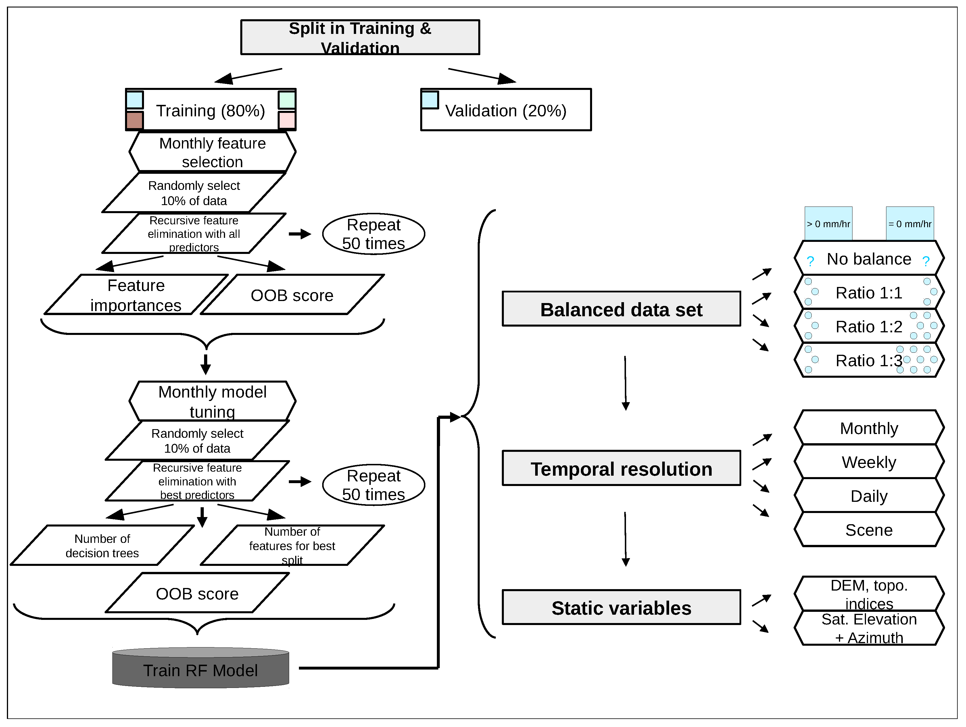
The feature selection and tuning were performed on a monthly basis, whereas the training was performed on a monthly, weekly, daily and scene based resolution. All of these temporal variations were also tested using a different amount of non-rainy pixels (unbalanced, ratio of 1:1, ratio1:2 and ratio of 1:3).

The results from the model training on a monthly and unbalanced selected pixel basis revealed the following model performance. The POD was very high ranging from 0.76–0.83 for the five test weeks and the POFD was very low at around 0.08. However, the FAR was very high (0.76 on average). The HSS was especially low in the less rainy seasons like May and September with values 0.15–0.25 and higher in the rainy months like June, July and August (0.37 on average). The PC was overall very high at 0.93 since most rainy pixels are recognized correctly by the model.

The POD was for all temporal resolutions stable and ranged from 0.73–0.87 with an unbalanced choice of pixels regarding all test weeks. When using the ratio of 1:1, the POD dropped for all temporal resolutions because this ratio highly overestimates the true distribution of rainfall data. The POD ranged between 0.22–0.41. We tested the ratio1:2 which resulted in a higher POD compared the ratio of 1:1 and a lower POD than the unbalanced choice (0.33–0.52). Training the RF models with a ratio of 1:3 led to a moderate POD of 0.40–0.61 for all temporal resolutions. The POFD was overall low for all tests ranging between 0.01–0.08.

The FAR decreased in all test weeks with increasing temporal resolution (e.g., from a monthly to weekly resolution) using the unbalanced option when training the RF model. Using the unbalanced choice of pixels, however, led to enormous high FAR up to 0.9. The FAR dropped rapidly when the models were trained using the ratio of 1:1. Modeling with the ratio of 1:1 led to an improvement of the FAR on all time scales which could be reduced down to 0.11. The FAR increased for all temporal scales when the models were trained using the ratio1:2 and ratio of 1:3. However, the POD in both cases was higher compared to the POD of the ratio of 1:1 at all temporal scales.

The HSS displays the overall performance of the model. The HSS increased when the temporal resolution decreased. This is due to the decreasing FAR with decreasing temporal resolution. The highest HSS was found when training the model on a scene basis. Regarding the amount of rainy pixels for training, we find that the HSS was highest when trained with the ratio of 1:3.

The PC was lowest for all temporal resolutions when the model is trained with a ratio of 1:1 (0.79–0.86). It increased for all test weeks with a ratio of 1:2 and reached very good results when the model is either trained unbalanced or with a ratio of 1:3 (up to 0.93). The PC in the unbalanced ratio was very high due to the many correctly negative classified pixels.

To summarize, we find that training the models on a scene basis together with the ratio of 1:3 performs best. This means that we choose all rainy pixels and the triple amount of non-rainy pixels for each scene separately. We also find that the results improve with increasing temporal resolution (see Figure 5).

Although other studies improved their model performance by the use of static predictors, we found that there is hardly any difference when training the model using static predictors on a scene basis with a ratio of 1:3 (see Figure 2 and Table 3). In order to test the effect of static predictors, we performed a separate feature selection and a separate RF parameter tuning on a monthly basis (see

Table 6. Comparison of scene based trained models with a ratio of 1:3 without and with the use of static predictors (SP).

Validation	May		June		July		August		September
	No SP	With SP	No SP	With SP	No SP	With SP	No SP	With SP	No SP	With SP
POD	0.47	0.41	0.57	0.55	0.59	0.59	0.61	0.55	0.57	0.48
POFD	0.03	0.03	0.03	0.03	0.04	0.04	0.04	0.03	0.02	0.02
FAR	0.29	0.30	0.26	0.24	0.26	0.25	0.26	0.24	0.23	0.25
HSS	0.49	0.44	0.59	0.58	0.59	0.60	0.60	0.57	0.60	0.53
PC	0.92	0.92	0.93	0.92	0.92	0.93	0.93	0.93	0.94	0.92

for the comparison).

Figure 6 displays the validation scores for the precipitation area delineation for 5–12 July 2017. There are some differences in the POD, FAR and HSS, but hardly any differences in the POFD and PC. The HSS is highest when the POD is high and the FAR low.

Figure 7 states that low precipitation rates (<10th percentile) are prone to errors with a relatively low POD and a high FAR, whereas high precipitation rates (>90th percentile) display a very POD (ca. 0.9), and a low FAR (ca. 0.2). The POD and HSS increase with increasing precipitation rates, whereas the FAR decreases with increasing precipitation rates.

A reason for that might be that clouds with low precipitation amounts do not differ much from non-precipitating clouds in terms of their top temperatures in the different channels. By contrast, the top cloud temperatures from clouds that lead to high amounts of precipitation can be distinguished more easily from the non-precipitating clouds because of the significant temperature differences.

3.2. Results of the Comparison between the New Precipitation Area Delineation and IMERG’s IR Only Precipitation

The best model was compared to the IR only product which uses only one spectral band for precipitation retrieval (see

Table 7. Comparison of the new precipitation area delineation (PAD) and IMERG’s IR only precipitation for the test weeks (May, June, July, August, September 2017).

Validation	May		June		July		August		September
	PAD	IR only	PAD	IR only	PAD	IR only	PAD	IR only	PAD	IR only
POD	0.40	0.07	0.58	0.29	0.59	0.28	0.55	0.28	0.50	0.26
POFD	0.03	0.07	0.03	0.06	0.04	0.06	0.03	0.06	0.02	0.05
FAR	0.35	0.99	0.24	0.55	0.27	0.43	0.26	0.51	0.25	0.52
HSS	0.43	0.002	0.59	0.22	0.60	0.25	0.56	0.23	0.54	0.23
PC	0.92	0.92	0.93	0.81	0.93	0.74	0.93	0.83	0.93	0.84

). Compared to IMERG’s IR only, the new precipitation delineation based on Elektro-L2 and Insat-3D displayed a higher POD (0.4–0.59) than IR only (0.24 on average) which highly underestimates precipitation events. The POFD of IR only is comparably low. The FAR is extremely high (between 0.43–0.99) compared to the new precipitation delineation. The HSS and partly the PC of IR only produce lower values (HSS at 0.19 and PC at 0.84 on average for all months), which stresses the improvement of the new multispectral delineation.

Figure 8 shows an example of a scene from 7 July 2017 at 4:00 p.m. UTC. Grey represents the MW swath where the gauge calibrated MW precipitation is available and no clouds occur. The white areas are masked out due to a low quality index below 0.9 which indicates that these areas could not be filled with gauge calibrated MW precipitation and therefore are probably snow or ice covered. The white areas cannot be used for training and validation. The colours yellow (TN), red (FN), blue (FP) and green (TP) indicate the verification measures. The left graphic depicts the performance of the new precipitation area delineation based on the gauge calibrated MW precipitation from IMERG.

The graphic on the right shows the differences in the IR only and gauge calibrated MW precipitation product for 7 July 2017 at 4:00 p.m. UTC on the TiP as an example. It indicates that IR only does not capture the precipitating areas which occur in the gauge calibrated MW precipitation product (FN) and also produces some False Positives (FP) where no precipitation occurred.

Our findings show that our model performs better than IR only precipitation compared to IMERG’s gauge calibrated MW precipitation.

Figure 9 distinguishes the modeling performance of IR only in low (<10th percentile), medium (between > 10th and < 90th percentile) and high (>90th percentile) precipitation rates. It reveals that high precipitation rates are easier to detect compared to low precipitation rates by IR only. The POFD is comparably low and the FAR decreases with high precipitation rates. The HSS increases with the increase in precipitation. The PC decreases in comparison from high to low precipitation rates.

4. Discussion

In this study we present the first rain area delineation on the TiP based on GEO satellite data which are fully validated across space and time.

Due to the missing IMERG independent gauge and weather radar network on the TiP, the variety of validation data are restricted. We therefore use the gauge calibrated MW precipitation from IMERG which was excluded from the feature selection, tuning and training processes to gain independent precipitation data.

Before modeling, we defined conditions for the selection of the data (see Section 2.3 RF model training and validation). When checking the data, we found pixels in the gauge calibrated MW precipitation of IMERG which are flagged as rainy but are not marked as cloudy in the Insat-3D cloud mask. Since they do not fulfill the condition of being cloudy in the cloud mask, they are excluded from training and validation. Some of these pixels were classified as probably cloudy in the cloud mask of Insat-3D. However, we decided to use only those pixels which were clearly classified as cloudy.

We also note that many pixels in all seasons, but especially in May and September, are frequently masked out due to IMERG’s quality index, which, in these cases, is below 0.9. The snow and ice covered areas are not used for precipitation retrieval. The IMERG algorithm adds IR information when MW is not able to produce reliable estimates due to the high reflectance of snow and ice. The IR reduces the quality of the precipitation estimates, which are then excluded from training and validation.

Due to computational effort, we performed the feature selection and RF parameter tuning only once; however, the results might change when performing a feature selection for all of the different settings of the models.

There are several possibilities for the failure of the precipitation area delineation. We find that the detection of high precipitation amounts (above 90th percentile) is quite well captured by the new precipitation delineation, whereas low precipitation (below 10th percentile) performs poorly. The medium range of precipitation (between 10th and 90th percentile) is better (worse) captured (1) than precipitation below (above) the 10th (90th) percentile and (2) in the rainy season. Our results indicate that low precipitation rates are hard to capture using GEO satellite data. The difference of the brightness temperatures between precipitating and non-precipitating pixels, especially for low precipitation rates, is not inconsistent and leads to false results. In addition, a high FAR indicates that the model is not able to sufficiently differ between precipitation and no precipitation. High precipitation rates are especially important regarding disaster management and water availability for humans.

Adding static predictors did not change our results. We assume that, due to the rather coarse monthly basis, the feature selection did not include many of the static predictors, which, therefore, did not change the results much.

Our study shows that precipitation area delineation works best in the rainy months (July, August). We found quite a poor performance for the rather dry months May and September. The precipitating areas in June are captured with intermediate accuracy.

We tested four different temporal resolutions and found that scene based trained models performed best. Coarse temporal resolutions like monthly trained models instead lead to worse results. Daily and weekly trained models performed at an intermediate level, with a better tendency of daily models to capture precipitation. Furthermore, we tested four different balancing methods when training the model. We found that there are differences in the performance when changing the balance of rainy and non-rainy pixels. Both tests changed the results which indicates that the data input highly affects the prediction outcome. Depending on the modeling approach, the training data should be selected carefully.

We use IMERG’s gauge calibrated MW precipitation for training and validation because it is the most reliable satellite precipitation product within IMERG [28]. However, it is restricted to those areas where MW is available. The gaps, where MW is not available, are filled in IMERG with IR based on one single band from GEO satellites. The indirect relation between IR and precipitation leads to an underestimation of precipitation. However, the IR is more frequently available compared to the MW precipitation. IMERG’s IR only product is not able to capture precipitation precisely.

We showed that our precipitation area delineation outperforms the IR only precipitation from IMERG. This is due to the very low POD (missing precipitation) and the very high FAR in the IR only product. We therefore conclude that multispectral IR information enhances the precipitation area classification results. Figure 10 displays the distribution of the validation measures covering the available data in 2017 (Figure 10a–d). There is hardly any pattern visible for TP, FP and FN, but the TN are found to mostly occur in the south of the TiP. The western part of the TiP contains frequently masked out areas covered with snow and ice leading to data gaps in all verification measures. The gauge calibrated MW precipitation totals (Figure 10e) and the frequency of gauge calibrated MW precipitation (Figure 10f) capture the dry western and some northern parts of the TiP, whereas the south and southeast are moist and influenced by (1) orographic effects and (2) the monsoon.

Other studies also focus on the classification of precipitating areas. To this end, the Meteosat Second Generation (MSG) Spinning Enhanced Visible and InfraRed Imager (SEVIRI) data with its resolution of 3 km and 15 min or the Himawari-8 with its 2 km and 15 min resolution are used several times for various areas [15,16,17,18,19,20,21]. Thies et al. [17] discriminate raining from non-raining cloud areas over Germany using MSG SEVIRI with reference to a German Weather radar product and found for night-time a POD of 0.6, a POFD of 0.2 and a FAR of 0.5. They also find comparable results for daytime. In their study about precipitation process and rainfall intensity differentiation, Thies et al. [18] use the detection of the precipitation areas together with the precipitation process to assign the precipitation rates. The POD varies between 0.1–0.7, whereas the POFD varies between 0–0.6, the FAR is between 0.3–0.9 and the HSS does not exceed 0.2. Kühnlein et al. [16] derive precipitation estimates from MSG SEVIRI using RF and find a POD of 0.5, POFD of 0.15, FAR of 0.5 and HSS of 0.2–0.5 for their classification of precipitating areas in Germany. Mapping rainfall over southern Africa using MSG SEVIRI lead to a validation aggregation of 1 h to a POD of 0.6, a low POFD of 0.18, but a high FAR of 0.8 and a low HSS of 0.18 [20].

Precipitating clouds were classified using IR from Himawari-8 where an enormous high POD of 0.98 and a high HSS of 0.2–0.8 is found, whereas the FAR does not exceed 0.01 [22]. Min et al. [21] estimate summertime precipitation from Himawari-8 and determine a POD of 0.58, a FAR between 0.27–0.41 and a HSS of 0.53. The TiP is especially challenging for satellite based precipitation retrieval techniques. This is due to the high elevation that causes low surface temperatures. These low surface temperatures hardly differ from the temperature of the clouds. This is problematic for the IR based techniques. On the other side, the high elevation and the semi-arid conditions are problematic for PMW sensors, since they often detect the ground signal in these cases which leads to misinterpretations in the retrieval algorithms. The same holds true for snow and ice covered areas which are very common on the TiP. Even if we use the best available data source within the IMERG product by choosing the MW based precipitation information as a reference for our technique, one has to keep in mind that this rainfall information should not be considered as the “truth” because of the described uncertainties.

GPM rainfall estimates are evaluated against gauge networks by Tan et al. [64] and their evaluation results in a POD of 0.7, FAR of 0.3-0.8 and a HSS of 0.3-0.7, whereas the data were evaluated on a precipitation threshold of 0.2 mm/hr. Everything below 0.2 mm/hr is not considered as precipitation because they state that small precipitation rates cannot be captured by satellites.

Table 8. Comparison of the validation measures of the new precipitation area delineation (PAD) compared to other studies.

Validation Measures	PAD	Thies et al., 2008a	Thies et al., 2008b	Kühnlein et al., 2014	Meyer et al., 2017a	Thus, & Shin 2018	Min et al., 2019
POD	0.52	0.6	0.1–0.7	0.5	0.6	0.98	0.58
POFD	0.03	0.2	0–0.6	0.15	0.18
FAR	0.27	0.5	0.3–0.9	0.5	0.8	0.01	0.27–0.41
HSS	0.54		>0.2	0.2–0.5	0.18	0.2–0.8	0.53
PC	0.92

summarizes the validation metrics of other studies compared to our results.

We use two GEO satellites to retrieve the precipitating area over the TiP. Future enhanced GEO systems from the Elektro-L series with a variety of spectral bands which can be operationally used will enhance the retrieval of precipitation over the TiP. In addition, possible minimal spatial offsets when superimposing the three different satellite products (Elektro-L2, Insat-3D, GPM IMERG) might be reduced. In addition, other studies indicate this issue [55,65].

The gauge calibrated MW precipitation combines imager and sounder which were all calibrated to the GPM core instrument (GMI). However, there are differences in the performance of precipitation detection in each sensor and especially in the differentiation between imager and sounder. There are two imagers (GMI, AMSR) and three sounders (ATMS, MHS, SSMIS) available in the V05B IMERG version. A sounder might perform worse than an imager, which then leads to a false classification [28]. The microwave humidity sounder (MHS) is known to strongly overestimate low rain rates and underestimate moderate intensities [28,36]. The MHS and the advanced temperature and moisture sounder (ATMS) are less accurate than the conical-scanning sensors like the GMI [66]. Since we would lose too much data when removing the sounder, we keep all data.

5. Conclusions

The lack of reliable precipitation data enhances the need for satellite-based precipitation retrievals for this region. Thus far, no precipitation retrieval especially for the TiP is available in a high spatio-temporal resolution. The aim of the study is to model the precipitation area delineation on the TiP using multispectral data from two GEO satellites (Insat-3D, Elektro-L2) with a machine learning approach (RF) based on the best quality gauge calibrated MW precipitation from IMERG. We showed that the precipitation area detection can be improved by (1) changing the ratio of the precipitating or non-precipitating data during training, and (2) by changing the temporal resolution to scene based trained models. Adding static predictors in the training process did not improve the precipitation area detection due to the coarse temporal resolution of the feature selection. We found a strong improvement of our multispectral precipitation area delineation compared to IMERG’s single band IR only precipitation estimate with reference to the gauge calibrated MW precipitation. Our multispectral approach overcomes the main weakness of IMERG’s IR only precipitation product, which underestimates precipitation [28].

References

1. Immerzeel, W.W.; van Beek, L.P.; Bierkens, M.F. Climate Change Will Affect the Asian Water Towers. Science 2010, 328, 1382–1385. [Google Scholar] [CrossRef] [PubMed]
2. Alazzy, A.A.; Lü, H.; Chen, R.; Ali, A.B.; Zhu, Y.; Su, J. Evaluation of Satellite Precipitation Products and Their Potential Influence on Hydrological Modeling over the Ganzi River Basin of the Tibetan Plateau. Adv. Meteorol. 2017, 2017, 3695285. [Google Scholar] [CrossRef]
3. Zhang, X.; Lu, X.; Wang, X. Comparison of spatial interpolation methods based on rain gauges for annual precipitation on the Tibetan plateau. Pol. J. Environ. Stud. 2016, 25, 1339–1345. [Google Scholar] [CrossRef]
4. He, H.Y.; Guo, Z.H.; Xiao, W.F.; Guo, Q.S. Mapping monthly precipitation for Tibetan Plateau with GIS and multivariate analysis based on DEM data. Acta Ecol. Sin. 2005, 25, 2933–2938. [Google Scholar]
5. Gerlitz, L.; Conrad, O.; Böhner, J. Large-scale atmospheric forcing and topographic modification of precipitation rates over High Asia—A neural-network-based approach. Earth Syst. Dyn. 2015, 6, 61–81. [Google Scholar] [CrossRef]
6. Karger, D.N.; Conrad, O.; Böhner, J.; Kawohl, T.; Kreft, H.; Soria-Auza, R.W.; Zimmermann, N.E.; Linder, H.P.; Kessler, M. Climatologies at high resolution for the earth’s land surface areas. Sci. Data 2017, 4, 1–20. [Google Scholar] [CrossRef] [PubMed]
7. Curio, J.; Maussion, F.; Scherer, D. A 12-year high-resolution climatology of atmospheric water transport over the Tibetan Plateau. Earth Syst. Dyn. 2015, 6, 109–124. [Google Scholar] [CrossRef] [Green Version]
8. Curio, J.; Scherer, D. Seasonality and spatial variability of dynamic precipitation controls on the Tibetan Plateau. Earth Syst. Dyn. 2016, 7, 767–782. [Google Scholar] [CrossRef] [Green Version]
9. Maussion, F.; Scherer, D.; Mölg, T.; Collier, E.; Curio, J.; Finkelnburg, R. Precipitation seasonality and variability over the Tibetan Plateau as resolved by the high Asia reanalysis. J. Clim. 2014, 27, 1910–1927. [Google Scholar] [CrossRef]
10. Bai, A.J.; Liu, C.H.; Liu, X.D. Diurnal Variation of Summer Rainfall over the Tibetan Plateau and Its Neighboring Regions Revealed by TRMM Multi-Satellite Precipitation Analysis. Chin. J. Geophys. 2008, 51, 518–529. [Google Scholar] [CrossRef] [Green Version]
11. Fu, Y.; Liu, G. Possible misidentification of rain type by TRMM PR over Tibetan Plateau. J. Appl. Meteorol. Climatol. 2007, 46, 667–672. [Google Scholar] [CrossRef]
12. Lehnert, L.W.; Wesche, K.; Trachte, K.; Reudenbach, C.; Bendix, J. Climate variability rather than overstocking causes recent large scale cover changes of Tibetan pastures. Sci. Rep. 2016, 6, 24367. [Google Scholar] [CrossRef] [PubMed] [Green Version]
13. Bookhagen, B.; Burbank, D.W. Topography, relief, and TRMM-derived rainfall variations along the Himalaya. Geophys. Res. Lett. 2006, 33, 1–5. [Google Scholar]
14. Yin, Z.Y.; Zhang, X.; Liu, X.; Colella, M.; Chen, X. An Assessment of the Biases of Satellite Rainfall Estimates over the Tibetan Plateau and Correction Methods Based on Topographic Analysis. J. Hydrometeorol. 2008, 9, 301–326. [Google Scholar] [CrossRef]
15. Kühnlein, M.; Appelhans, T.; Thies, B.; Nauss, T. Improving the accuracy of rainfall rates from optical satellite sensors with machine learning—A random forests-based approach applied to MSG SEVIRI. Remote Sens. Environ. 2014, 141, 129–143. [Google Scholar] [CrossRef]
16. Kühnlein, M.; Appelhans, T.; Thies, B.; Nauß, T. Precipitation estimates from MSG SEVIRI daytime, nighttime, and twilight data with random forests. J. Appl. Meteorol. Climatol. 2014, 53, 2457–2480. [Google Scholar] [CrossRef]
17. Thies, B.; Nauss, T.; Bendix, J. Discriminating raining from non-raining cloud areas at mid-latitudes using meteosat second generation SEVIRI night-time data. Meteorol. Appl. 2008, 15, 219–230. [Google Scholar] [CrossRef]
18. Thies, B.; Nauss, T.; Bendix, J. Discriminating raining from non-raining clouds at mid-latitudes using meteosat second generation daytime data. Atmos. Chem. Phys. 2008, 8, 2341–2349. [Google Scholar] [CrossRef] [Green Version]
19. Thies, B.; Nauss, T.; Bendix, J. Precipitation process and rainfall intensity differentiation using Meteosat Second Generation Spinning Enhanced Visible and Infrared Imager data. J. Geophys. Res. Atmos. 2008, 113, 1–19. [Google Scholar] [CrossRef]
20. Meyer, H.; Drönner, J.; Nauss, T. Satellite-based high-resolution mapping of rainfall over southern Africa. Atmos. Meas. Tech. 2017, 10, 2009–2019. [Google Scholar] [CrossRef] [Green Version]
21. Min, M.; Bai, C.; Guo, J.; Sun, F.; Liu, C.; Wang, F.; Xu, H.; Tang, S.; Li, B.; Di, D.; et al. Estimating Summertime Precipitation from Himawari-8 and Global Forecast System Based on Machine Learning. IEEE Trans. Geosci. Remote Sens. 2019, 57, 2557–2570. [Google Scholar] [CrossRef]
22. Thus, D.; Shin, D.B. Classification of precipitating clouds using satellite infrared observations and its implications for rainfall estimation. Q. J. R. Meteorol. Soc. 2018, 144, 133–144. [Google Scholar] [Green Version]
23. Upadhyaya, S.; Ramsankaran, R. Modified-INSAT Multi-Spectral Rainfall Algorithm (M-IMSRA) at climate region scale: Development and validation. Remote Sens. Environ. 2016, 187, 186–201. [Google Scholar] [CrossRef]
24. Joyce, R.J.; Janowiak, J.E.; Arkin, P.A.; Xie, P. CMORPH: A Method that Produces Global Precipitation Estimates from Passive Microwave and Infrared Data at High Spatial and Temporal Resolution. J. Hydrometeorol. 2004, 5, 487–503. [Google Scholar] [CrossRef]
25. Behrangi, A.; Hsu, K.l.; Imam, B.; Sorooshian, S.; Huffman, G.J.; Kuligowski, R.J. PERSIANN-MSA: A Precipitation Estimation Method from Satellite-Based Multispectral Analysis. J. Hydrometeorol. 2009, 10, 1414–1429. [Google Scholar] [CrossRef]
26. Ashouri, H.; Hsu, K.; Sorooshian, S.; Braithwaite, D.; Knapp, K.; Cecil, D.; Nelson, B.; Prat, O. PERSIANN-CDR: Daily precipitation climate data record from multisatellite observations for hydrological and climate studies. Bull. Am. Meteorol. Soc. 2015, 96, 69–83. [Google Scholar] [CrossRef]
27. Kidd, C.; Levizzani, V. Status of satellite precipitation retrievals. Hydrol. Earth Syst. Sci. 2011, 15, 1109–1116. [Google Scholar] [CrossRef] [Green Version]
28. Tan, J.; Petersen, W.A.; Tokay, A. A Novel Approach to Identify Sources of Errors in IMERG for GPM Ground Validation. J. Hydrometeorol. 2016, 17, 2477–2491. [Google Scholar] [CrossRef]
29. Wu, L.; Zhai, P. Validation of daily precipitation from two high-resolution satellite precipitation datasets over the Tibetan Plateau and the regions to its east. Acta Meteorol. Sin. 2012, 26, 735–745. [Google Scholar] [CrossRef]
30. Tong, K.; Su, F.; Yang, D.; Hao, Z. Evaluation of satellite precipitation retrievals and their potential utilities in hydrologic modeling over the Tibetan Plateau. J. Hydrol. 2014, 519, 423–437. [Google Scholar] [CrossRef]
31. Gao, Y.; Liu, M. Evaluation of high-resolution satellite precipitation products using rain gauge observations over the Tibetan Plateau. Hydrol. Earth Syst. Sci. 2013, 17, 837–849. [Google Scholar] [CrossRef] [Green Version]
32. Huffman, G.J.; Bolvin, D.T.; Nelki, E.J.; Nelkin, E.J. Integrated Multi-satellitE Retrievals for GPM (IMERG) Technical Documentation; 2017; pp. 1–48. Available online: https://pmm.nasa.gov/sites/default/files/document_files/IMERG_doc.pdf (accessed on 1 October 2019).
33. Guo, H.; Chen, S.; Bao, A.; Behrangi, A.; Hong, Y.; Ndayisaba, F.; Hu, J.; Stepanian, P.M. Early assessment of Integrated Multi-satellite Retrievals for Global Precipitation Measurement over China. Atmos. Res. 2016, 176–177, 121–133. [Google Scholar] [CrossRef]
34. Ning, S.; Wang, J.; Jin, J.; Ishidaira, H. Assessment of the Latest GPM-Era High-Resolution Satellite Precipitation Products by Comparison with Observation Gauge Data over the Chinese Mainland. Water 2016, 8, 481. [Google Scholar] [CrossRef]
35. Grecu, M.; Olson, W.S.; Munchak, S.J.; Ringerud, S.; Liao, L.; Haddad, Z.; Kelley, B.L.; Mclaughlin, S.F. The GPM combined algorithm. J. Atmos. Ocean. Technol. 2016, 33, 2225–2245. [Google Scholar] [CrossRef]
36. Kidd, C.; Matsui, T.; Chern, J.; Mohr, K.; Kummerow, C.; Randel, D. Global precipitation estimates from cross-track passive microwave observations using a physically based retrieval scheme. J. Hydrometeorol. 2016, 17, 383–400. [Google Scholar] [CrossRef]
37. Tan, M.; Duan, Z. Assessment of GPM and TRMM Precipitation Products over Singapore. Remote Sens. 2017, 9, 720. [Google Scholar] [CrossRef]
38. Xu, R.; Tian, F.; Yang, L.; Hu, H.; Lu, H.; Hou, A. Ground validation of GPM IMERG and TRMM 3B42V7 rainfall products over southern Tibetan Plateau based on a high-density rain gauge network. J. Geophys. Res. 2017, 122, 910–924. [Google Scholar] [CrossRef]
39. Ma, Y.; Tang, G.; Long, D.; Yong, B.; Zhong, L.; Wan, W.; Hong, Y. Similarity and error intercomparison of the GPM and its predecessor-TRMM multisatellite precipitation analysis using the best available hourly gauge network over the Tibetan Plateau. Remote Sens. 2016, 8, 569. [Google Scholar] [CrossRef]
40. Bookhagen, B.; Burbank, D.W. Toward a complete Himalayan hydrological budget: Spatiotemporal distribution of snowmelt and rainfall and their impact on river discharge. J. Geophys. Res. Earth Surf. 2010, 115, 1–25. [Google Scholar] [CrossRef]
41. National Satellite Meteorological Centre. Insat-3D Data Products Catalog; Technical Report; 2014. Available online: http://satellite.imd.gov.in/dynamic/INSAT3D_Catalog.pdf (accessed on 1 October 2019).
42. MOSDAC, Space Applications Centre, Indian Space Research Organisation, Govt. of INDIA. Meteorological & Oceanographic Satellite Data Archival Centre. Available online: https://www.mosdac.gov.in/ (accessed on 1 October 2019).
43. News, S.P. INSAT-3D Now Operational. 2014. Available online: https://www.wmo-sat.info/vlab/2014/02/insat-3d-now-operational/ (accessed on 1 October 2019).
44. Zak, A. Zenit Delivers Elektro-L2. 2016. Available online: http://www.russianspaceweb.com/elektro-l2.html (accessed on 30 September 2019).
45. Skofronick-Jackson, G.; Huffman, G.; Stocker, E.; Petersen, W. Successes with the Global Precipitation Measurement (GPM) Mission, Technical Report 4. In Proceedings of the International Geoscience and Remote Sensing Symposium (IGARSS), Beijing, China, 10–15 July 2016. [Google Scholar]
46. Huffman, G. GPM IMERG Final Precipitation L3 Half Hourly 0.1 Degree x 0.1 Degree V05 (3IMERGHH), Greenbelt, MD, Goddard Earth Sciences Data and Information Services Center (GES DISC). 2017. Available online: https://disc.gsfc.nasa.gov/datasets/GPM_3IMERGHH_V05/summary (accessed on 1 October 2019).
47. Huffman, G.J. Precipitation Measurement Mission. GPM Data Downloads. Available online: https://pmm.nasa.gov/data-access/downloads/gpm (accessed on 30 September 2019).
48. ORNL DAAC. Digital Elevation Model: Global 30 Arc-Second Elevation Data Set (GTOPO30); 2017. Available online: https://webmap.ornl.gov/ogc/dataset.jsp?dg_id=10003_1 (accessed on 1 October 2019).
49. Jenness, J. Topographic Position Index (TPI) v. 1.2. Technical Report. 2006. Available online: http://www.jennessent.com/downloads/TPI_Documentation_online.pdf (accessed on 30 September 2019).
50. Riley, S.J.; DeGloria, S.D.; Elliot, R. A Terrain Ruggedness Index that Quantifies Topographic Heterogeneity. Intermt. J. Sci. 1999, 5, 23–27. [Google Scholar]
51. Wilson, M.F.; O’Connell, B.; Brown, C.; Guinan, J.C.; Grehan, A.J. Multiscale terrain analysis of multibeam bathymetry data for habitat mapping on the continental slope. Mar. Geod. 2007, 30, 3–35. [Google Scholar] [CrossRef]
52. Egli, S.; Thies, B.; Drönner, J.; Cermak, J.; Bendix, J. A 10 year fog and low stratus climatology for Europe based on Meteosat Second Generation data. Q. J. R. Meteorol. Soc. 2017, 143, 530–541. [Google Scholar] [CrossRef]
53. Huffman, G. IMERG Quality Index. Available online: https://docserver.gesdisc.eosdis.nasa.gov/public/project/GPM/IMERG_QI.pdf (accessed on 30 September 2019).
54. Breiman, L. Random Forests. Mach. Learn. 2011, 45, 5–32. [Google Scholar] [CrossRef]
55. Meyer, H.; Lehnert, L.W.; Wang, Y.; Reudenbach, C.; Nauss, T.; Bendix, J. From local spectral measurements to maps of vegetation cover and biomass on the Qinghai-Tibet-Plateau: Do we need hyperspectral information? Int. J. Appl. Earth Obs. Geoinf. 2017, 55, 21–31. [Google Scholar] [CrossRef]
56. Breiman, L. Out-of-Bag Estimation; Statistics Department. University of California: Berkeley, CA, USA, 1996; pp. 1–13. Available online: https://scholar.google.com/scholar?hl=en&as_sdt=0%2C5&as_vis=1&q=Out-of-Bag+Estimation%3B+Statistics+Department.+University+of+California.+Berkeley.&btnG= (accessed on 1 October 2019).
57. Pedregosa, F.; Varoquaux, G.; Gramfort, A.; Michel, V.; Thirion, B.; Grisel, O.; Blondel, M.; Prettenhofer, P.; Weiss, R.; Dubourg, V.; et al. Scikit-learn: Machine Learning in Python. J. Mach. Learn. Res. 2011, 12, 2825–2830. [Google Scholar]
58. Ghaemi, M.; Feizi-Derakhshi, M.R. Feature selection using Forest Optimization Algorithm. Pattern Recognit. 2016, 60, 121–129. [Google Scholar] [CrossRef]
59. Cermak, J. SOFOS—A New Satellite-Based Operational Fog Observation Scheme. Ph.D. Thesis, Philipps-Universität Marburg, Marburg, Germany, 2006. [Google Scholar]
60. World Weather Research Program/Working Group On Numerical Experimentation Joint Working Group On Verification. Forecast Verification—Issues, Methods and FAQ. Available online: https://www.cawcr.gov.au/projects/verification/ (accessed on 30 September 2019).
61. Beusch, L.; Foresti, L.; Gabella, M.; Hamann, U. Satellite-based rainfall retrieval: From generalized linear models to artificial neural networks. Remote Sens. 2018, 10, 939. [Google Scholar] [CrossRef]
62. Yamamoto, M.K.; Ueno, K.; Nakamura, K. Comparison of Satellite Precipitation Products with Rain Gauge Data for the Khumb Region, Nepal Himalayas. J. Meteorol. Soc. Jpn. 2011, 89, 597–610. [Google Scholar] [CrossRef] [Green Version]
63. Kidd, C.; Tan, J.; Kirstetter, P.E.; Petersen, W. Validation of the Version 05 Level 2 precipitation products from the GPM Core Observatory and constellation satellite sensors. Q. J. R. Meteorol. Soc. 2018, 144, 313–328. [Google Scholar] [CrossRef]
64. Tan, J.; Petersen, W.A.; Kirchengast, G.; Goodrich, D.C.; Wolff, D.B. Evaluation of Global Precipitation Measurement Rainfall Estimates against Three Dense Gauge Networks Three Dense Gauge Networks. J. Hydrometeorol. 2018, 19. [Google Scholar] [CrossRef]
65. Yao, Z.; Li, W.; Zhao, B.; Chen, Y. Remote Sensing of Precipitation on the Tibetan Plateau Using the TRMM Microwave Imager. J. Appl. Meteorol. 2001, 40, 1381–1392. [Google Scholar] [CrossRef]
66. Li, R.; Wang, K.; Qi, D. Validating the Integrated Multisatellite Retrievals for Global Precipitation Measurement in Terms of Diurnal Variability With Hourly Gauge Observations Collected at 50,000 Stations in China. J. Geophys. Res. Atmos. 2018, 123, 10423–10442. [Google Scholar] [CrossRef]
Figure 1. Data availability of the least common data of Insat-3D, Elektro-L2 and GPM IMERG (with all met conditions) for the half year of 2017 on a temporal (a) and spatial (b) scale relative to the number of available scenes.
Remotesensing 11 02302 g001
Figure 2. Schematic view of the processing scheme of the precipitation area delineation.
Remotesensing 11 02302 g002
Figure 3. Workflow of the selection of the best model. See Section 2.4 for a detailed description.
Remotesensing 11 02302 g003
Figure 4. Average feature importance and standard deviations relative to the most important feature of the feature space. Feature importance was calculated for a subset of all available scenes from the training data set using all non-static predictors. The error bars were calculated based on one standard deviation of each predictor.
Remotesensing 11 02302 g004
Figure 5. Receiver Operating Characteristics (ROC) diagram comparing the probability of detection (POD) with the false alarm ration (FAR) based on the mean prediction samples of all test weeks in 2017. The colors / shape indicate the different temporal resolutions/different balanced data sets.
Remotesensing 11 02302 g005
Figure 6. Performance of the precipitation area delineation for eight days (5–12 July 2017) as boxplots. The validation scores are calculated for each validation scene of these eight days. The boxes display the 25th, 50th and 75th percentiles. Whiskers indicate extreme data up to 1.5 times of the interquartile range. Outliers are marked as crosses. The width of the boxes is relative to the available number of validation scenes.
Remotesensing 11 02302 g006
Figure 7. Performance of the new precipitation area delineation for July 2017 as boxplots for low, medium and high precipitation amounts according to percentiles. The boxes display the 25th, 50th and 75th percentiles. Whiskers indicate extreme data up to 1.5 times of the interquartile range. Outliers are marked as crosses. The width of the boxes is relative to the available number of validation scenes.
Remotesensing 11 02302 g007
Figure 8. Comparison of the performance of the new precipitation area delineation (left) with IMERG’s IR only, both with reference to IMERG’s gauge calibrated MW precipitation on July 7th 2017 on 4:00 p.m. UTC. These estimates are available for the grey MW swath marked area. Snow covered areas do not fulfill the quality index from IMERG.
Remotesensing 11 02302 g008
Figure 9. Performance of the precipitation area delineation using IR only precipitation for July 2017 as boxplots for low, medium and high precipitation rates according to percentiles. The boxes display the 25th, 50th and 75th percentiles. Whiskers indicate extreme data up to 1.5 times of the interquartile range. Outliers are marked as crosses. The width of the boxes is relative to the available number of validation scenes.
Remotesensing 11 02302 g009
Figure 10. Distribution of mean validation measures over the Tibetan Plateau (TiP) for 2017 (ad) with the precipitation totals (e) and frequency of gauge calibrated MW precipitation for 2017 (f).
Remotesensing 11 02302 g010