Article

Use of Very High-Resolution Optical Data for Landslide Mapping and Susceptibility Analysis along the Karnali Highway, Nepal

1
Goddard Earth Sciences Technology and Research, Universities Space Research Association, Columbia, MD 21046, USA
2
Hydrological Sciences Laboratory, NASA Goddard Space Flight Center, Greenbelt, MD 20771, USA
*
Author to whom correspondence should be addressed.
Remote Sens. 2019, 11(19), 2284; https://doi.org/10.3390/rs11192284
Submission received: 30 August 2019 / Revised: 19 September 2019 / Accepted: 25 September 2019 / Published: 30 September 2019
(This article belongs to the Section Remote Sensing in Geology, Geomorphology and Hydrology)

Abstract

:
The Karnali highway is a vital transport link and the only primary roadway that connects the remote Karnali region to the lowlands in Mid-Western Nepal. Every year there are reports of landslides blocking the road, making this area largely inaccessible. However, little effort has focused on systematically identifying landslides and landslide-prone areas along this highway. In this study, landslides were mapped with an object-based approach from very high-resolution optical satellite imagery obtained by the DigitalGlobe constellation in 2012 and PlanetScope in 2018. Landslides ranging from 10 to 30,496 m2 were detected within a 3 km buffer along the highway. Most of the landslides were located at lower elevations (between 500–1500 m) and on steep south-facing slopes. Landslides tended to cluster closer to the highway, near drainage channels and away from faults. Landslides were also most prevalent within the Kuncha Formation geologic class, and the forested and agricultural land cover classes. A susceptibility map was then created using a logistic regression methodology to highlight patterns in landslide activity. The landslide susceptibility map showed a good prediction rate with an area under the curve (AUC) of 0.90. A total of 33% of the study arealies in high/very high susceptibility zones. The map highlighted the lower elevated areas between Bangesimal and Manma towns with the Kuncha Formation geologic class as being the most hazardous. The banks of the Karnali River, its tributaries and areas near the highway were also highly susceptible to landslides. The results highlight the potential of very high-resolution optical imagery for documenting detailed spatial information on landslide occurrence, which enables susceptibility assessment in remote and data scarce regions such as the Karnali highway.

1. Introduction

The mountains in Nepal are one of the most hazardous environments in the world, with frequent landslides caused by tectonic activity, monsoonal rainfall and infrastructure development [1]. About 72% of the country is hilly or mountainous, with 50% of the total population residing in these areas [2]. Long-term development and economic prosperity of this region is contingent on the availability and reliability of roads for access to infrastructure such as marketplaces, schools, and hospitals [3]. As a result, understanding the frequency, distribution, and susceptibility of landslides along Nepal’s main transportation corridors is vital for better characterizing the impact that landslides may impose on the population within this region.
The Karnali region (Figure 1) in Mid-Western Nepal has a high poverty rate, low social development, weak governance and high development costs due to inaccessibility [4]. Food insecurity is a major problem in this region [5]. The Karnali highway is the only major transportation link that connects Jumla district in the Karnali region to Surkhet district, which contains the provincial capital. Construction of the highway started in 1991 and is still ongoing under Nepal’s Road Sector Development Project with support from the World Bank [6]. Every year, there are reports of highway blockade by landslides, particularly during the monsoon season that spans June through September, making this area inaccessible by road [7]. Despite the known landslide frequency, there have been no systematic landslide inventories conducted along this highway to date. In order to safeguard the livelihood of the people, ensure sustained development in this region and the proper functioning of the highway, areas prone to landslides must be identified and, ultimately, the risk must be mitigated.
Landslide susceptibility maps provide an estimate of where landslides might occur, typically based on knowledge of landslides that have occurred in the past [8]. There are many different methods for conducting landslide susceptibility mapping depending on the objectives of the resulting map [9]. Landslide susceptibility mapping can be categorized as heuristic, deterministic and statistical [10]. Heuristic methods are based on expert knowledge, hence are subjective. Deterministic approaches require a large number of input data gathered from laboratory tests and field visits, and can only be applied in smaller areas [11]. Statistical approaches are based on relationships between known or inferred instability variables with past and present distributions of landslides [12]. Similarly in Nepal, various landslide susceptibility mapping methods have been tested and their performances have been documented [13,14,15,16,17,18,19,20,21,22,23,24,25,26,27,28,29]. Most of these studies have been conducted in Central and Eastern Nepal, possibly due to the lack of landslide data in the Western part of the country.
The most important information required for susceptibility mapping is an inventory of past landslide occurrences. Conventional landslide inventories are produced by field visits and aerial photo interpretation [30]. This process is very time-consuming and can be subjective [31,32]. Recent advancements in remote-sensing technologies have significantly increased our ability to rapidly map landslides of various sizes, with less in situ surveys or human interaction [33,34,35]. Remote sensing of landslides can be categorized into two groups: pixel-based and object-based image analysis (OBIA). Pixel-based methods utilize spectral information alone, and ignore spatial information [36]. Hence, these are not the best method to map geomorphic processes such as landslides [37]. OBIA, on the other hand, incorporates spectral, textural, morphological and topographical characteristics, which are more suitable for detecting landslides [38]. OBIA has been successfully used to map landslides all around the world [37,39,40,41,42,43,44,45,46,47,48,49,50,51,52,53,54,55,56,57]. Comparative studies between pixel-based methods and OBIA have highlighted the superiority of OBIA in detecting landslides with fewer false positives [58,59].
Landsat 8, with a spatial resolution of 30 m, has been found effective in mapping larger landsides for rapid assessment in Nepal [60,61,62,63]. The launch of Sentinel-2, with a spatial resolution of 10 m in 2015, has also increased the availability of free high-resolution optical imagery and enabled landslide detection at finer scales than what was possible with previous open source satellite imagery from Landsat and ASTER. However, hazard and risk studies require a complete landslide inventory, and freely available optical imagery from sensors such as Sentinel-2, Landsat and ASTER are not capable of detecting small landslides with areas of less than 100 m2. As a result, very high-resolution (VHR) imagery is the only space-based option for a systematic and comprehensive landslide mapping [64]. VHR satellites are commercially owned, expensive and not freely available, except when disaster charters (www.disasterscharter.org) are activated. NextView licensing agreement, a partnership between the U.S. government and U.S. commercial vendors, provides access to VHR imagery for federal agencies in support of scientific research [65]. This partnership provides access to VHR optical imagery obtained from the DigitalGlobe (DG) (Westminster, Colorado, USA) constellation. The Small Satellite Data Buy program [66] is another initiative started by NASA to investigate the effectiveness of VHR imagery in support of research activities undertaken by the agency. This program provides access to additional VHR optical imagery from three satellites: SkySat, RapidEye and PlanetScope, operated by Planet Labs Inc. (San Francisco, California, USA) for NASA funded projects.
The aim of this study is to create multi-temporal landslide inventories along the Karnali highway using VHR imagery from DG and PlanetScope with the OBIA methodology. The effectiveness of this remote sensing based landslide inventory is demonstrated by producing a susceptibility map, documenting its predictive capacity and potential applications.

2. Study Area

The Karnali highway (Figure 1) in Province 6 of Nepal runs south to north starting at Bangesimal in the Surkhet District and ending in Khalanga, of the Jumla District. This highway mostly runs parallel to the Karnali river between Bangesimal and Manma. Beyond Manma, it follows the Tila river, a tributary of the Karnali river. Since we are interested in landslide activity that might affect the highway, we defined a buffer of 3 km along the highway as our study area. The route is 233 km long and paved. Construction of the highway started in 1991/1992. However, the road was finally opened along the entire route to Khalanga only on 1 April 2007.
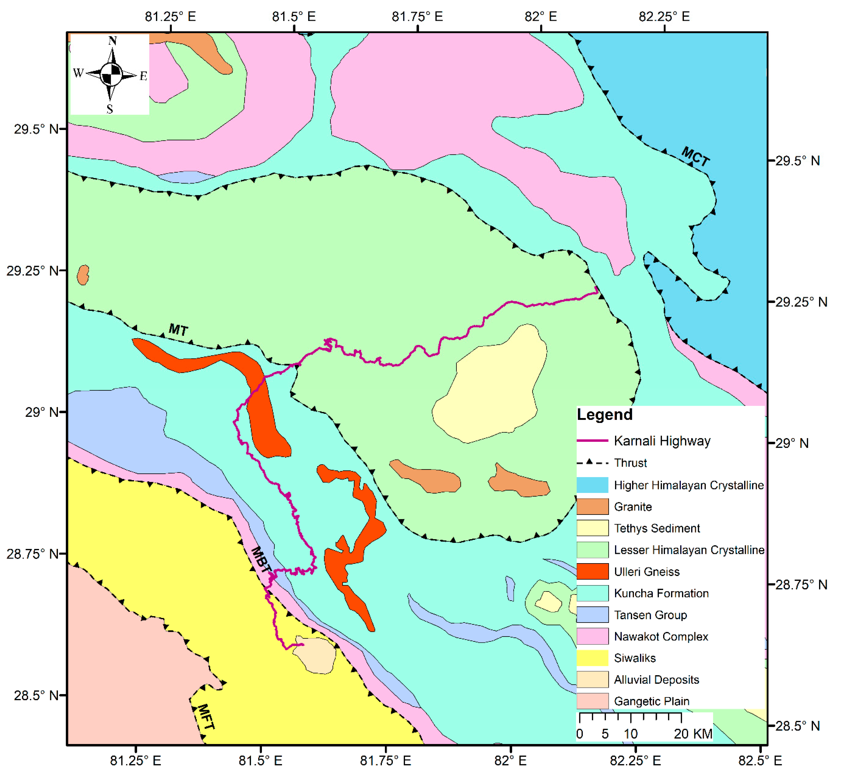
Nepal is divided into five geotectonic zones from south to north: the Gangetic Plain, Siwaliks, Lesser Himalaya, Higher Himalaya and Tibetan-Tethys Himalaya. These zones are separated from each other by the thrust faults. The southernmost fault, the Main Frontal Thrust (MFT) separates the Siwaliks from the Gangetic Plain. The Main Boundary Thrust (MBT) separates the Lesser Himalaya from the Siwaliks. The Main Central Thrust (MCT) separates the Higher Himalaya from the Lesser Himalaya. The South Tibetan Detachment System (STDS) marks the boundary between the Higher Himalaya and the overlying fossiliferous sequence of the Tibetan-Tethys Himalaya. The Karnali highway passes through two geotectonic zones: the Siwaliks and the Lesser Himalaya (Figure 2). The Neogene Siwaliks consists of mudstone, sandstone and conglomerate. The Lesser Himalayan rocks mainly consist of low to medium grade Proterozoic metamorphic rocks (e.g., phyllite, schist, metasandstone and quartzite) of the Kuncha Formation along with metasedimentary rocks of the Nawakot Complex that extend from MBT at the southern margin to MCT at the northern margin. The granitic intrusions are also present within the Lesser Himalayas, such as the Ulleri Gneiss. The Gondwana rocks and Post-Gondwana Eocene-Early Miocene sediments of the Tansen group are present sporadically throughout the Lesser Himalayas. The Lesser Himalayan Crystalline, consisting of Proterozoic gneisses and schists, are present in the Lesser Himalayas as klippe.

3. Materials and Methods

3.1. Data

3.1.1. Satellite Imagery

Multispectral data from three satellites of the DG constellation: GeoEye-1 (GE01), QuickBird-2 (QB02) and WorldView-2 (WV02) (Table 1) and PlanetScope [68] were used for creating the landslide inventories. The DG satellites acquire images over a certain area only when it is tasked and at various off-nadir angles. VHR imagery tends to be best if the off-nadir angle is <20° [64]. Images acquired with higher off-nadir angles will suffer from image distortion and result in lower georeferencing accuracies. We queried the DG archives for images with off-nadir angle <20° and cloud cover <20%. The satellite coverage over this area was intermittent, with nearly complete coverage available only for the year 2012. In order to complete the coverage, we incorporated one frame from 2010, two frames from 2011 and two frames from 2013 (Figure 1). As most of the images are from 2012, we will consider landslides detected using DG as a 2012 inventory. DG Level 1B products are available through the NextView license [65]. DG level 1B data are radiometrically and sensor corrected, but not projected to a plane using map projection or datum [69]. We orthorectified the data using a 30 m NASADEM [70] and then converted into top-of-the-atmosphere reflectance for normalized difference vegetation index (NDVI) calculations. All the processing was done using Polar Geospatial Center’s orthorectification tools [71] on the Advanced Data Analytics Platform (ADAPT) at NASA Goddard Space Flight Center (GSFC)’s NASA Center for Climate Simulation (NCCS) (http://www.nccs.nasa.gov/services/adapt).
In order to map recent landslides, we created another landslide inventory (referred to as the 2018 inventory) using 22 PlanetScope tiles from 11 and 12 November 2018, covering the whole highway. We used Level 3B PlanetScope Ortho Scene products at 3 m resolution with tile size of 24 km by 7 km.

3.1.2. Landslide Explanatory Variables

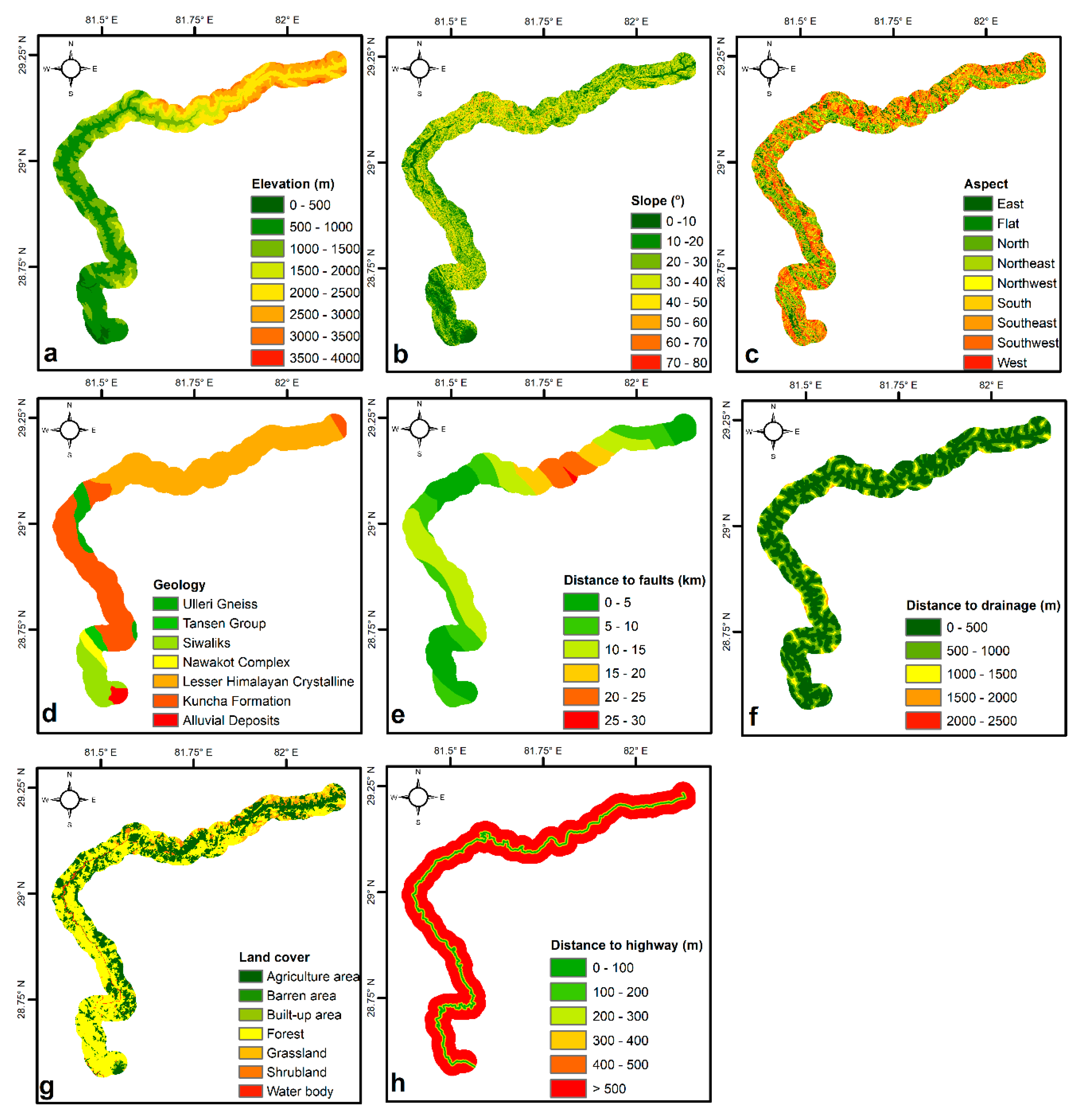
The explanatory variables (Figure 3) used in this study can be categorized into four main groups: topographical, geological, hydrological and anthropogenic. These variables were generated in raster format with spatial resolution of 30 m in ArcGIS.
Topographical variables considered in this study are elevation, slope and aspect and were generated using a 30 m NASADEM. Elevation controls most of the geomorphological and geological processes and ranges across the study region from 341 to 3753 m. The elevation was classified into eight classes (Figure 3a). Slope is often considered the most important factor contributing to landslides [72] and varies from 0 to 75° over the study area. The slope was classified into eight classes (Figure 3b). Slope aspect determine the amount of insolation and rainfall received due to prevailing climatologic patterns, which can have a substantial influence on landslide triggering [73]. The slope aspect was prepared with values ranging from 0 to 360 and further classified into nine classes (Figure 3c).
Geology plays an important role in the occurrences of landslides as lithological and structural variations often lead to a difference in rock strength and permeability of soils and rocks [74,75]. Geological variables were obtained from digitized geological map from the Department of Mines and Geology in Nepal [67]. The Karnali highway passes through seven geological classes (Figure 3d). The main geological structures that demarcate the study area are the MBT and the Mahabharat Thrust (MT) (Figure 2). These fault lines were digitized from the geological map. Distance to faults were created using the Euclidean distance toolset in ArcGIS and classified into six classes (Figure 3e).
The hydrological variable was represented by distance to drainage, since runoff adversely affects stability by eroding the slope or by saturating the lower portion of the hillslope [76]. Drainage was obtained from NASADEM using hydrology toolset in ArcGIS. Distance to drainage was calculated using the Euclidean distance method and classified into five classes (Figure 3f).
Anthropogenic variables were represented by land cover and distance to highway. Human activities and road construction along steep mountain terrain destabilize the slope, which can increase the frequency of landslides [77]. Land cover with seven land cover types (Figure 3g) was obtained from the 2010 land cover map created from Landsat at 30 m resolution by The International Centre for Integrated Mountain Development (ICIMOD) [78]. Road networks data were obtained from OpenStreetMap [79]. The distance to highway was created using the Euclidean distance method and classified into six classes (Figure 3h).

3.2. Methods

3.2.1. Landslide Inventory Mapping

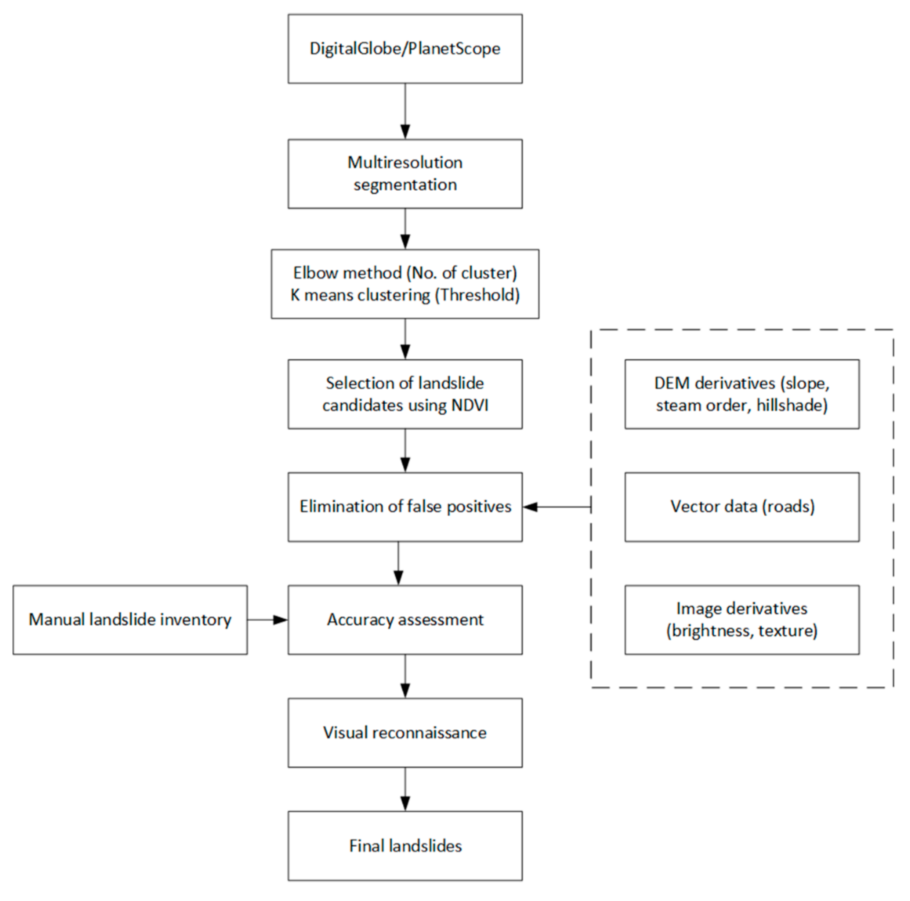
The methodology for landslide mapping is outlined in Figure 4. Imagery used in this study have different dates and acquisition modes. Hence, the methodology described below has been applied to individual tiles of DG and PlanetScope separately. The steps are described in sequential order.

Segmentation

The first important procedure is segmentation, which divides an image into objects based on the homogeneity of the pixel values [80]. We used multiresolution segmentation (MRS) [81] available in eCognition® Developer 8.9 (Trimble Germany GmbH, Munich, Germany) software [82]. MRS is a bottom-up region-merging technique in which small objects are merged into bigger ones in subsequent steps [83]. MRS requires three parameters: scale, shape and compactness. The scale controls the image object size, with higher scale resulting in larger objects and small scale in smaller objects. The shape determines the degree to which shape influences segmentation vs. spectral homogeneity. The compactness defines the weight of compactness criteria. The higher the value, more compact the objects will be. There are many methods for selecting the optimal scale automatically, such as estimation of scale parameter 2 [84], plateau objective function [42] and optimal scale parameter selector [85]. However, currently there is no standardized or best method for optimal scale estimation [86]. Manual trial and error selection of scale parameter is time consuming. Different scales were tested for segmentation, but obtaining a scale that accounts for different sizes of landslides present in the region was very difficult. Generally, over-segmentation is preferred to under-segmentation as merging is possible in later steps [37]. Hence, to ensure that the boundaries of the smallest landslide areas were derived, we used a small scale parameter of 10 with shape 0.1 and compactness 0.9 [37,57].

Selection of Likely Landslide Candidate Objects

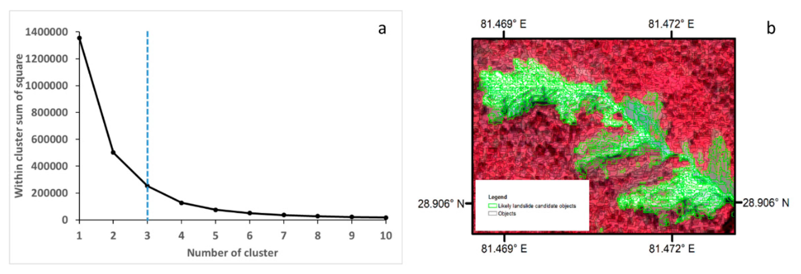
In this study, landslides and false positives (non-landslide areas appearing/initially classified as landslides) were detected first, with sequential elimination of false positives in the subsequent step. A NDVI threshold was used to separate likely landslide candidate objects from other vegetated surfaces. This threshold is selected according to Martha et al. [41] using K-means clustering [87]. K-means clustering finds cluster centers in continuous data, which can be used to set thresholds for identification of landslides and removal of false positives. One requirement of this method is that the number of clusters (K) must be predefined. We used the Elbow method to calculate the number of clusters (Figure 5a). This method was implemented in Python. In the Elbow method, a graph is plotted between within-cluster sum of squares (WCSS), which is the distance between each member of the cluster and its centroid and number of clusters. The main idea behind K-means clustering is to group data such that the WCSS is at a minimum. The location of bend (elbow) in the plot indicates the appropriate number of clusters beyond which increasing the number of clusters will not result in a decrease of WCSS. The elbow point was then determined automatically using the Elbow point detection method [88,89]. Using the obtained number of clusters, a NDVI threshold was obtained using K-means clustering to select likely landslide candidate objects (Figure 5b).

Removal of False Positives from Landslides

Since NDVI was used as a distinguishing feature, objects with similar or lower NDVI values, such as shadows, rivers, roads, buildings, agricultural and barren lands, are misclassified as landslides. Combination of local knowledge, K-means clustering and spatial datasets were used for elimination of these false positives in sequential order.
Candidate objects belonging to shadow class were separated using brightness and hillshade. The hillshade map was generated using solar altitude and azimuth information at the time of image acquisition in ArcGIS. Shadows have low brightness and hillshade. K-means clustering was then used to obtain thresholds for brightness and hillshade. River objects were separated using stream order obtained from Strahler’s method [90]. Stream order >5 represents perennial flowing water body. Candidate objects that intersected high stream orders were assigned to river class. As water exhibits negative NDVI, a threshold of NDVI < 0 was also used as additional criteria to separate river. Alluvial sands are present closer to river channels and are brighter than landslides. Hence, candidate objects belonging to this class were separated using the distance from river and higher brightness values compared to surrounding gorges. Distance to river and brightness threshold were set manually according to local conditions. Candidate objects that intersected the roads vector layer were separated and assigned to the road class. Agricultural land such as terrace farming was separated based on low slope and texture values, which was calculated using the gray level co-occurrence matrix (GLCM) [37]. Mean GLCM of the red band was calculated using Haralick’s method [91]. The mean GLCM threshold was obtained from K-means clustering. Buildings were removed using shape criteria (i.e., small area and rectangular fit). Barren areas appeared darker than landslides, so a manual brightness threshold was selected to differentiate objects belonging to the barren class from landslide objects. A visual check to remove remaining obvious false positives was achieved in under 15 min. The remaining objects were merged and exported from eCognition in shapefiles as final landslides for validation and further analysis in ArcGIS.

3.2.2. Landslide Susceptibility Mapping

In this study we used logistic regression to calculate susceptibility, which allows for a multivariate regression between a dependent variable and several independent variables [92]. In landslide susceptibility mapping, the dependent variable is binary, representing the presence or absence of landslides, and the independent variables are landslide explanatory variables. The independent variables can be continuous, categorical or a combination of both [93]. The generalized linear model function in R software was used to fit the logistic regression model. In logistic regression, the logit function converts the probabilities into values from 0 to 1. The function that defines probability of landslide occurrence ( P ) is defined as:
logit = log ( P 1 P ) = b 0 + b 1 x 1 + b 2 x 2 + + b n x n ,
and
P = 1 1 + e ( b 0 + b 1 x 1 + b 2 x 2 + + b n x n ) ,
where, x i are the explanatory variables considered by the model, b 0 is the intercept and b i the coefficients assigned to each explanatory variable x i .

4. Results

4.1. Landslide Mapping Validation

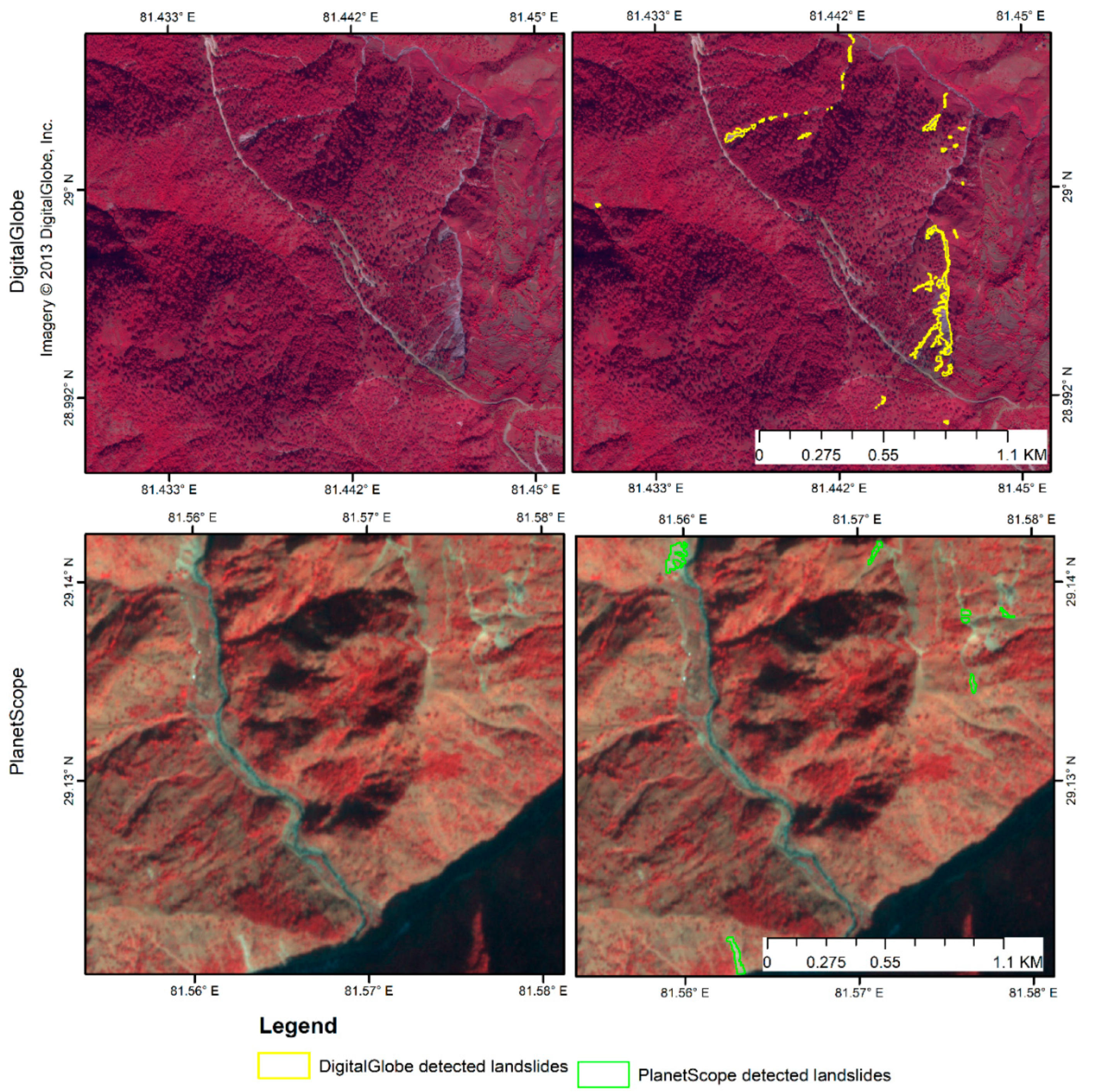
Figure 6 shows two example areas for the OBIA-detected landslides from DG and PlanetScope images. In order to validate the OBIA-detected landslides, the inventory was compared with a reference inventory that was compiled manually, using one WV02 image from 8 October 2012 (red square in Figure 1). Three metrics were calculated: true positive (TP), false negative (FN), and false positive (FP). These metrics were not based on the number of landslides because segmentation-derived image objects rarely correspond to single landslides due to over or under-segmentation [53,94]. Instead, the performance metrics were determined according to the overlapping area. TPs are correctly mapped landslides; FPs are detected landslides that have not been mapped in the reference inventory and FNs are reference landslides not identified by OBIA. Based on these metrics, the two accuracy indices, producer accuracy (PA) also known as detection percentage, and user accuracy (UA) were calculated as follows:
P A = T P T P + F N 100
U A = T P T P + F P 100
It was observed that the OBIA-based method was only successful in obtaining 59% of the area of the reference inventory (Table 2). When evaluating based on the intersection of any portion of the reference and OBIA landslides, a PA of 98% was obtained. This suggests that nearly all landslides were detected using OBIA, but that the areas were not always accurate and had the tendency to be underestimated.

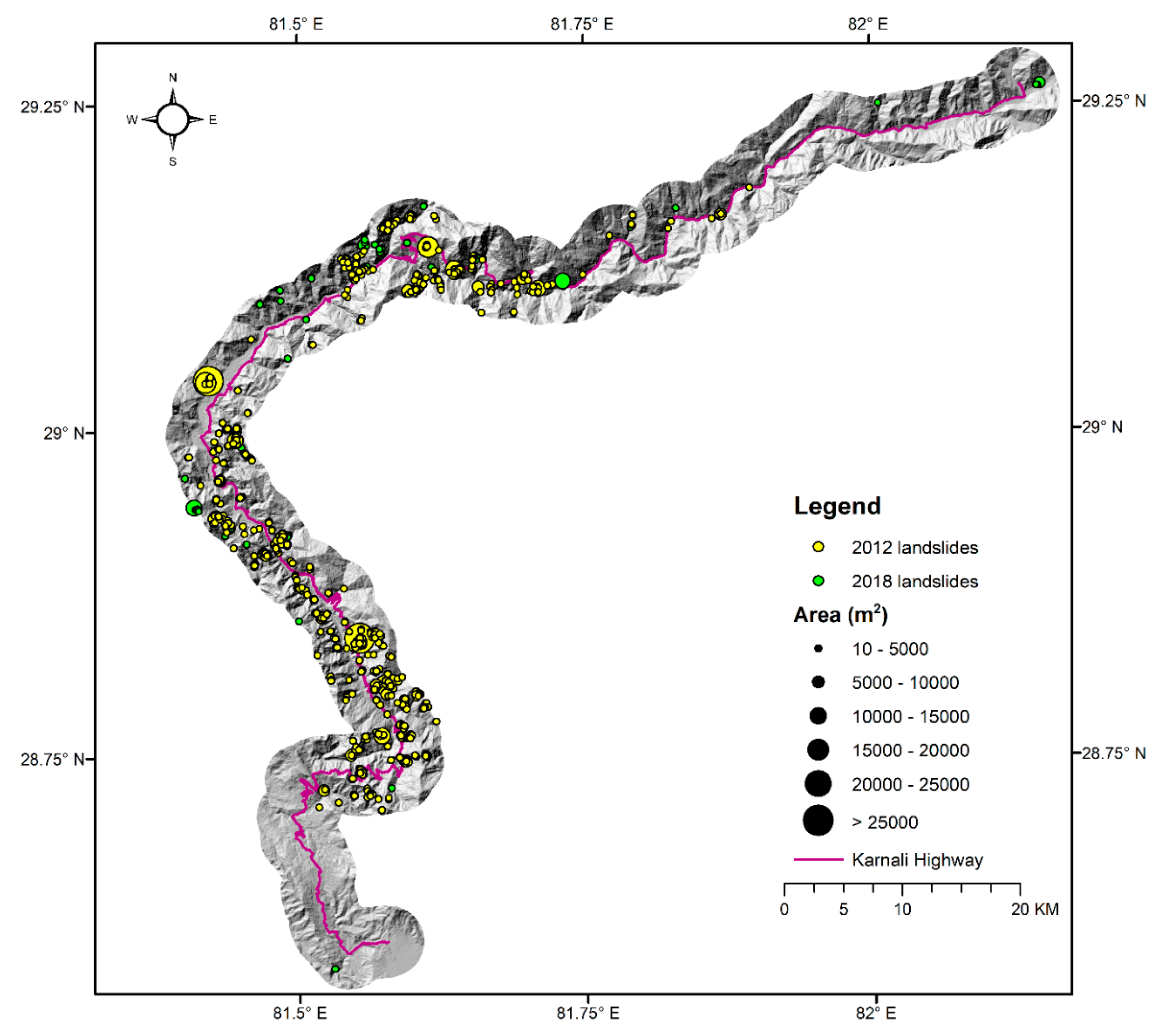
4.2. Spatial Distribution of Landslides

Figure 7 shows the location and size of OBIA-based landslides within the 980 km2 Karnali highway study area. The size of the landslides varied from 10 to 30,496 m2. As OBIA was not successful in delineating the complete area of individual landslides, and also to avoid spatial autocorrelation of landslide samples during susceptibility modelling [95,96], we converted the detected landslides into initiation points using a Digital Elevation Model (DEM). The initiation point was assumed to be the highest elevation on the landslide boundary. In total, 1061 landslide initiation points were generated. A total of 993 landslide initiation points were generated from landslide areas obtained from DG images between 2010–2013 and an additional 68 new landslide initiation points were generated using new landslide areas obtained from PlanetScope images from 2018.
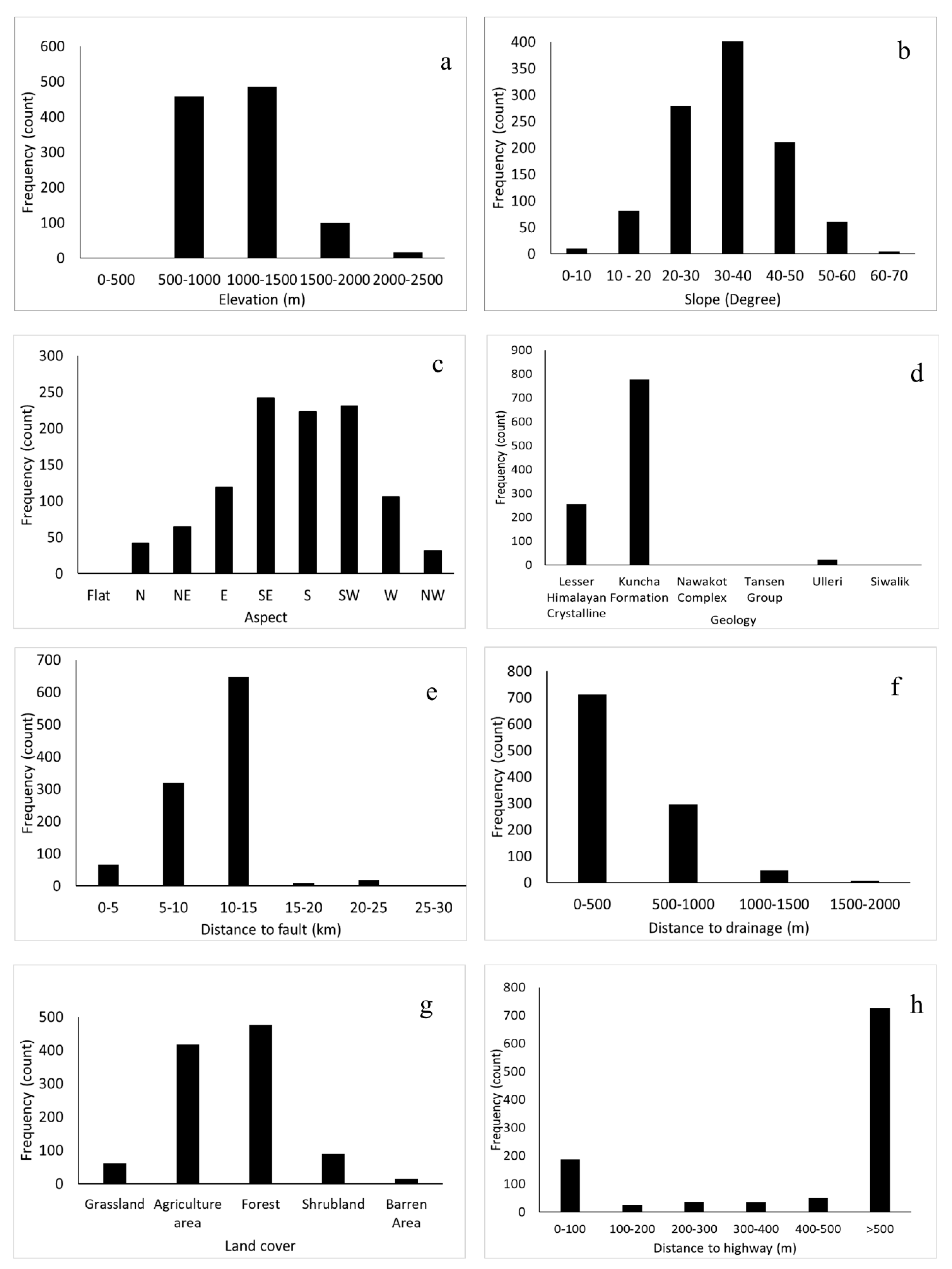
Figure 8 shows the relationship of landslides with explanatory variables. Most of the landslides are located between 500–1500 m in elevation (Figure 8a) with slopes of 20–50° (Figure 8b). Landslides are predominantly distributed within south-facing slopes (Figure 8c) that have high insolation and evaporation rates, resulting in less vegetated surfaces [73]. These slopes are also on the windward side, which tends to receive more precipitation compared to leeward slopes and might result in more landslide activity. The phyllite, schist, metasandstone and quartzite of the Kuncha Formation geologic class contains the majority of the landslides (Figure 8d). The phyllite of the Kuncha Formation are moderately to highly weathered and fractured [97], which might lead to increased landsliding. Landslides are located at a distance of 10–15 km from faults (Figure 8e), with the dominant fault zones oriented east–west. The effects of runoff and undercutting by the river are highlighted by a higher number of landslides within 500 m of drainages (Figure 8f). Comparison with the 2010 land cover map reveals landslides predominantly occur in forest and agriculture land cover types (Figure 8g), which might be due to destruction of forest for settlement and agriculture, as the development of the highway continued throughout the years. A higher number of landslides within 100 m of the highway (Figure 8h) suggests landslide initiation could be exacerbated due to infrastructure development associated with the highway.

4.3. Landslide Susceptibility and Validation

Different approaches exist for separating the landslide inventory into a training and validation data set. It is commonly suggested that approximately 20% of the data selected at random should be used to validate the result [95]. In this study, 75% of the landslide points selected randomly were used for training the logistic regression model and 25% were held for validation. An equal number of non-landslide points were also used during the training phase.
Eight landslide explanatory variables were considered for logistic regression. Aspect, geology and land cover are categorical variables and elevation, slope, distance to faults, distance to highway and distance to drainage are continuous variables. All the explanatory variables were classified into different classes with nominal values. In this study, each of the classes within the variables were represented using landslide densities and these values were used for logistic regression. Use of landslide densities also allows for the representation of explanatory variables on the same scale, which enables us to estimate the effect of each variables on landslide occurrence [98]. Landslide density [99] was calculated as:
L a n d s l i d e   D e n s i t y = ( B i / A i ) ( B / A )
where B i is the number of landslides within a class, A i is number of pixels in a class, B is the total number of landslides and A is total number of pixels within the study area.
Table 3 shows the regression coefficients along with test statistics of the eight explanatory variables. Standard error is the upper and lower limits of the coefficient. The z value is the ratio of regression coefficient to standard error. Pr(>|z|) is the significance. From the analysis of coefficients and test statistics, it is seen that all variables except for distance to drainage have a prominent role in landslide formation, highlighted by the positive coefficient and significance at 0.05 level. Slope with the highest coefficient has a higher effect on landslide formation than any other variable.
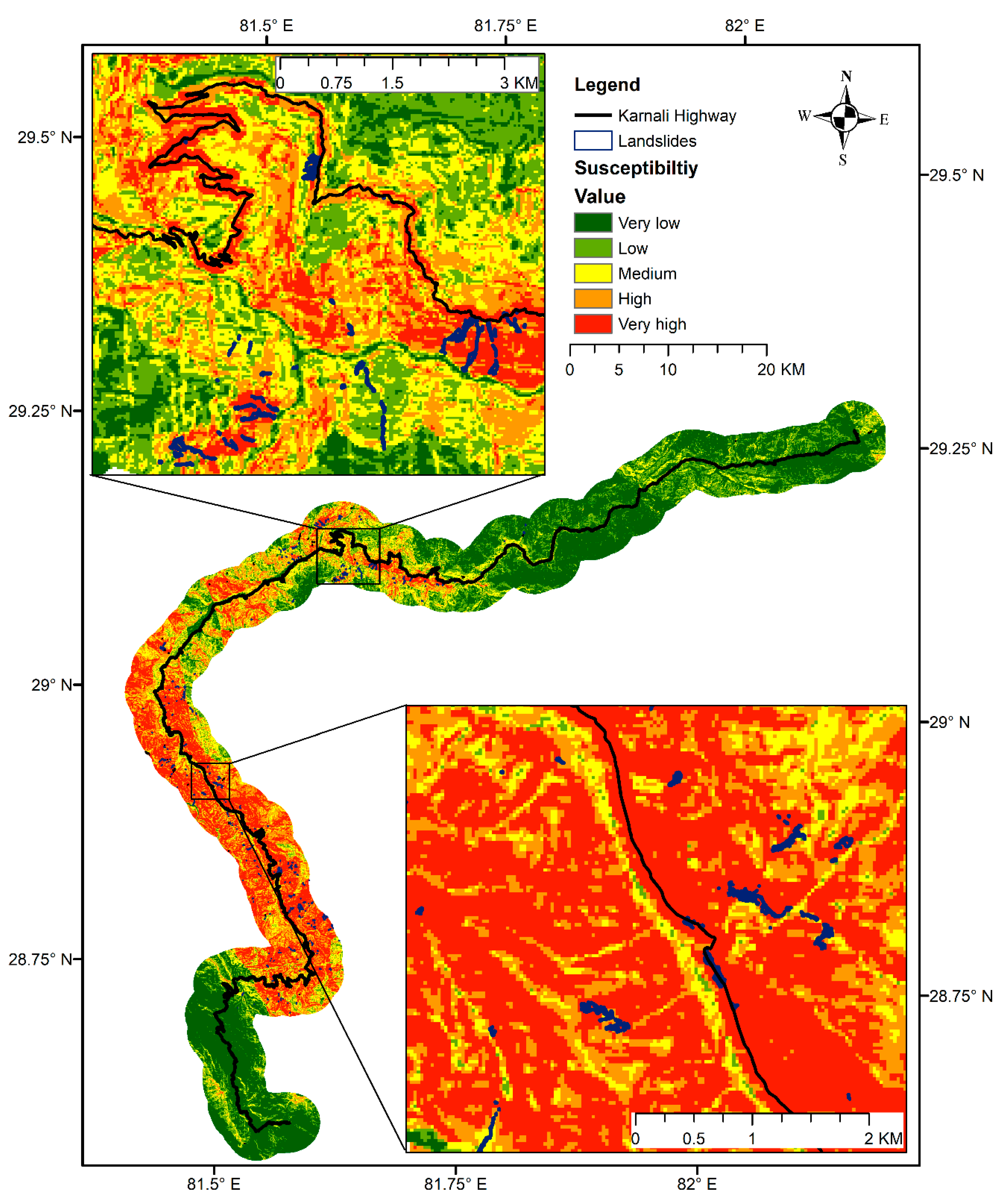
The susceptibility values obtained from logistic regression are probabilities on a continuous scale from 0 to 1. These values are classified into five levels: very low, low, moderate, high and very high (Figure 9) using the natural breaks algorithm [100], which groups similar values together maximizing the difference between classes. Table 4 shows the percentage of landslide susceptibility classes for the whole study area. A total of 53.58% of the area lies in the very low/low susceptibility zones, whereas 32.97% of the study area lies in the high/very high susceptibility zones. The map shows the lower elevation areas between Bangesimal and Manma towns (Figure 1), with the Kuncha Formation geologic class being the most hazardous. The banks of the Karnali River, its tributaries and areas near to the highway are also highly susceptible to landslides.
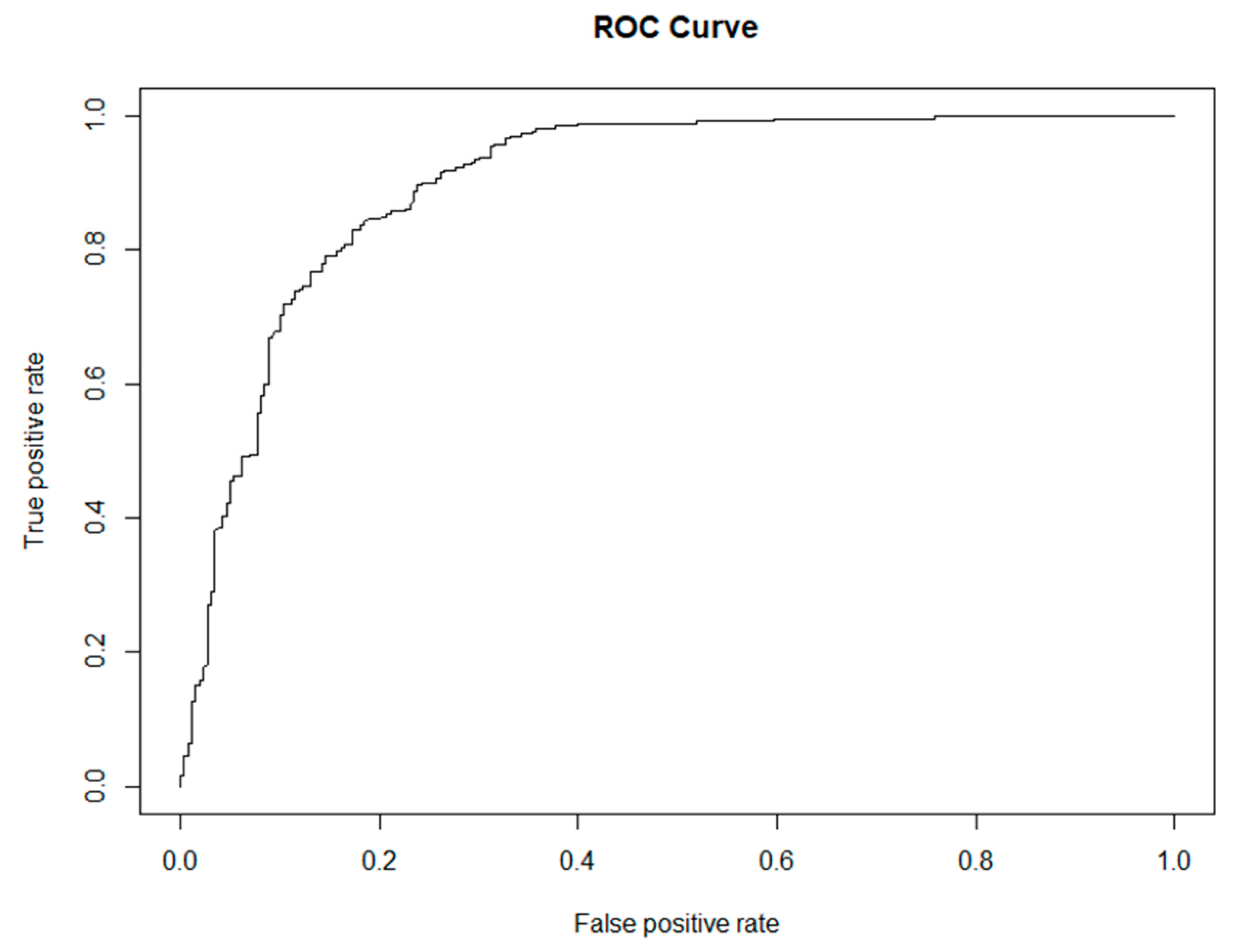
The landslide susceptibility map was verified with the receiver operating characteristic (ROC) curve statistics, a useful method for representing the quality of deterministic and probabilistic detection and forecast systems [101]. The ROC curve is created by plotting the true positive rate and false positive rate of each possible binary classification of a dataset [102]. The area under the curve (AUC) indicates the performance of the model. Its value ranges from 0 to 1, where 1 indicates a perfect model fit and 0.5 indicates that the model does not perform any better than random chance. A total of 259 landslides and an equal number of non-landslide points not used for training the logistic regression model were used for validating the landslide susceptibility map. Results of the ROC analysis shown in Figure 10 give an AUC value of 0.90, which is higher than the 0.7 suggested for a successful prediction [103].

5. Discussion

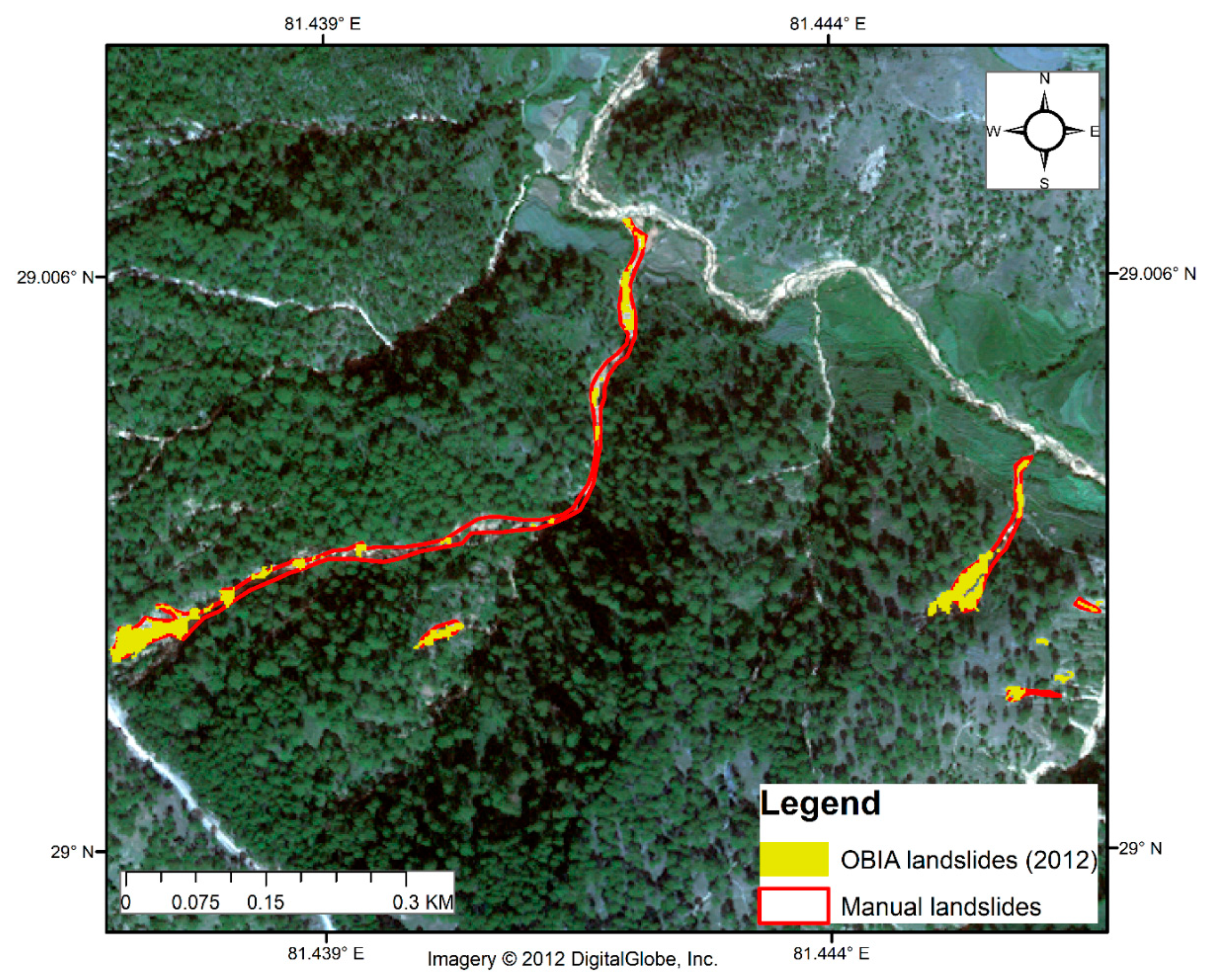
This study represents the first time VHR imagery was applied using the OBIA methodology to map landslides along the Karnali highway. This method was only successful in mapping 59% of the landslide areas relative to the reference inventory. Upon close investigation (Figure 11), it was noted that the OBIA based method was successful in delineating landslide scarps, but was unable to detect long narrow debris trails due to the lack of distinct spectral properties. A similar result and issue was reported while mapping landslide hotspots in New Zealand using OBIA [94]. Error may have been introduced by using the 30 m DEM, the single segmentation scale used for identification of the landslide candidates, and the removal of false positives in this study. The OBIA detected landslide inventory accuracy decreases gradually with the reduction of DEM resolution [104]. Most of the studies using OBIA for landslide detection utilized a high-resolution DEM (10 m and higher) created from sources such as stereo pairs [37], LiDAR [47] and contours [38]. Another factor contributing to the error might be the single segmentation scale used in this study. Multiple scale-based false positive identifications significantly improves the overall accuracy [42]. However, creating a DEM and using multiple segmentation scale OBIA landslide detection for areas as large as the entire Karnali highway is a challenge.
A total of 1161 initiation points were obtained based on landslide areas delineated from VHR imagery. In this study, we did not address amalgamation (i.e., mapping of several adjacent landslides as a single landslide) that might have occurred during merging and exporting from eCognition. However, amalgamation must be addressed if landslide inventories obtained using OBIA are to be utilized for studies where individual characteristics of a landslide are of importance, such as assessment of area–frequency distributions and estimation of landslide volumes [105,106]. A hybrid approach that combines OBIA with manual improvement could streamline the whole mapping process with acceptable accuracy, and reduce the time and effort needed for generating landslide inventories [94]. In mountainous areas, shadow is a major problem. Landslides that lie within shadows cannot be detected using optical imagery. Hence, field validation and inclusion of those landslides missed, because of this issue and the OBIA methodology in general, must be prioritized.
Based on initiation points, a landslide susceptibility map was produced using logistic regression. Although a good prediction rate (AUC value of 0.90) was achieved, some inherent problems related to the statistical method remain. The landslide inventory contains all types of landslides. Hence, the susceptibility map produced is highly generalized. Training the model for each landslide type might result in a slightly different susceptibility map that may be more suitable for local scale analysis. Use of initiation points may lead to underestimation of the hazard, as it does not consider size or runout of the landslide. Similarly, small landslides are assigned the same weight as larger landslides, which may result in a shift towards higher susceptibility further up on the slope [107]. Logistic regression is based on the assumption that past combinations of explanatory variables that have resulted in landslides in some area holds true in other areas as well. However, finding the optimal combination of variables is not always straightforward [108]. The training data only included landslide information from a 3 km buffer along the highway, which might not sufficiently capture all variable combinations responsible for landslide occurrence. Thus, some critical slopes might not be identified as highly susceptible zones. In order to avoid these scenarios, continuous monitoring and updating of the susceptibility map must be prioritized. Nevertheless, this study shows that remote sensing and the OBIA methodology is valuable for detecting landslides in a short amount of time in order to systematically characterize landslide pattern and improve our ability to identify susceptible zones in remote regions such as the Karnali highway in Mid-Western Nepal.
This study established landslide locations and areas along the Karnali highway for the first time. Approximately 33% of the study area lies in high/very high susceptibility zones. The road section that lies between Bangesimal and Manma towns is highly susceptible to landslides. This spatial and areal distribution will be helpful for decision makers to focus on locations with higher densities of landslide activity. There may be additional opportunities to further characterize slow moving landslides by considering displacement rates obtained from synthetic aperture radar (SAR) [49,109]. However, in mountainous regions such as Karnali, shadow, layover and decorrelation due to vegetation and snow, are factors limiting the applicability of SAR [110]. The 30 m susceptibility map provides estimates of locations where landslides might initiate and does not model landslide flow and deposition. Thus, it cannot be used for land-use planning, emergency response and engineering decisions directly. It can be used to provide a general overview of landslide hazard in the area and to delineate areas that might benefit from low-cost slope stabilization measures such as bioengineering [111,112]. These preventive measures not only help minimize landslide occurrence but also protect the population from its cascading impacts. While the susceptibility map proposed here is static, it can be used with dynamic variables such as satellite precipitation [113] to create a hazard map and identify sections of the highway that may be more likely to be exposed to landslides each season or with particular extreme rain events. However, this would require improved temporal information on when landslides occurred. Continuous monitoring of landslides and their evolution in time may be possible with recent availability of free high-resolution imagery from Sentinel-2 however, the resolution remains too coarse to resolve smaller landslide events. Additional information on population from Landscan [114] or Gridded Population of the World [115] can be used to better understand the potential exposure and risks to populations within the region.

6. Conclusions

A landslide inventory was created from VHR imagery in 2012 and 2018 using OBIA within a 3 km buffer of the Karnali highway. To our knowledge, this is the first landslide inventory in this area. The OBIA method was able to identify 59% of the landslide area obtained from manual mapping. The primary reason for the mismatch in landslide area was due to the challenge in detecting landslide tail or runout. Using landslide initiation points derived from the OBIA-based inventory area as training data, a landslide susceptibility map with a spatial resolution of 30 m was created using logistic regression. The map has a good prediction rate, with an AUC of 0.90. Results indicate that approximately 33% of the study area lies in high/very high susceptibility zones. The road section between Bangesimal and Manma was found to be the most hazardous. This susceptibility map provides the first estimates of highly susceptible areas to landslides along the Karnali highway, which can inform decisions about where to apply mitigation approaches, such as bioengineering. This method demonstrates the potential for conducting similar analyses in remote areas, providing the first step towards hazard and risk estimates and can be expanded to other landslide-prone regions around the country.

Author Contributions

P.A. and D.K. designed the research. P.A. performed object-based landslide mapping, susceptibility analysis and wrote the manuscript with support from T.S., D.K. and T.S. contributed to general discussion and review of the paper.

Funding

This research funded by National Aeronautics and Space Administration (NASA) High Mountain Asia Grant (NNX16AT79G) was further augmented with funds provided by NASA’s Small Satellite Data Buy (SSDB) program.

Acknowledgments

We would like to thank Paul Montesano for providing access to the eCognition software. Geospatial support for this work provided by the Polar Geospatial Center under (NNX16AT79G). Map data copyrighted OpenStreetMap contributors and available from https://www.openstreetmap.org.

Conflicts of Interest

The authors declare no conflict of interest.

References

  1. Petley, D.N.; Hearn, G.J.; Hart, A.; Rosser, N.J.; Dunning, S.A.; Oven, K.; Mitchell, W.A. Trends in landslide occurrence in Nepal. Nat. Hazards 2007, 43, 23–44. [Google Scholar] [CrossRef]
  2. Central Bureau of Statistics Nepal Population and Housing Census 2011. Available online: https://cbs.gov.np/wp-content/upLoads/2019/07/pulationandhousing-census-2011.pdf (accessed on 13 April 2018).
  3. Sapkota, J.B. Access to infrastructure and human well-being: Evidence from rural Nepal. Dev. Pract. 2018, 28, 182–194. [Google Scholar] [CrossRef]
  4. Ligal, P.R. Karnali Area Development: A Strategic Frame-Work. Available online: http://prad-nepal.com/wp-content/uploads/2015/09/Karnali-area-development-Strategic-framework1.pdf (accessed on 20 March 2018).
  5. World Food Programme A Sub-Regional Hunger Index for Nepal. Available online: http://neksap.org.np/uploaded/resources/Publications-and-Research/Reports/A Sub-Regional Hunger Index for Nepal, July 2009.pdf (accessed on 13 April 2018).
  6. Ahmed, F.; Regmi, P.P. Study on the Transport Constrains in Western Nepal (Karnali Highway Transport Corridor). Available online: http://archive.rapnepal.com/report-publication/study-transport-constrains-western-nepal-karnali-highway-transport-corridor (accessed on 3 April 2018).
  7. World Food Programme More than Roads: Using Markets to Feed the Hungry in Nepal. Available online: http://www.cashlearning.org/downloads/resources/documents/more-than-roads_using-markest-to-feed-the-hungry-in-nepal-_july-2010.pdf (accessed on 20 March 2018).
  8. Guzzetti, F.; Reichenbach, P.; Cardinali, M.; Galli, M.; Ardizzone, F. Probabilistic landslide hazard assessment at the basin scale. Geomorphology 2005, 72, 272–299. [Google Scholar] [CrossRef]
  9. Ercanoglu, M.; Gokceoglu, C. Use of fuzzy relations to produce landslide susceptibility map of a landslide prone area (West Black Sea Region, Turkey). Eng. Geol. 2004, 75, 229–250. [Google Scholar] [CrossRef]
  10. Aleotti, P.; Chowdhury, R. Landslide hazard assessment: Summary review and new perspectives. Bull. Eng. Geol. Environ. 1999, 58, 21–44. [Google Scholar] [CrossRef]
  11. Van Westen, C.J. Geo-information tools for landslide risk assessment: An overview of recent developments. Landslides Eval. Stab. 2004, 1, 39–56. [Google Scholar]
  12. Guzzetti, F.; Carrara, A.; Cardinali, M.; Reichenbach, P. Landslide hazard evaluation: A review of current techniques and their application in a multi-scale study, Central Italy. Geomorphology 1999, 31, 181–216. [Google Scholar] [CrossRef]
  13. Kayastha, P.; Dhital, M.R.; De Smedt, F. Landslide susceptibility mapping using the weight of evidence method in the Tinau watershed, Nepal. Nat. Hazards 2012, 63, 479–498. [Google Scholar] [CrossRef]
  14. Kayastha, P. Application of fuzzy logic approach for landslide susceptibility mapping in Garuwa sub-basin, East Nepal. Front. Earth Sci. 2012, 6, 420–432. [Google Scholar] [CrossRef]
  15. Kayastha, P.; Dhital, M.R.; De Smedt, F. Evaluation of the consistency of landslide susceptibility mapping: A case study from the Kankai watershed in east Nepal. Landslides 2013, 10, 785–799. [Google Scholar] [CrossRef]
  16. Kayastha, P.; Bijukchhen, S.M.; Dhital, M.R.; De Smedt, F. GIS based landslide susceptibility mapping using a fuzzy logic approach: A case study from Ghurmi-Dhad Khola area, Eastern Nepal. J. Geol. Soc. India 2013, 82, 249–261. [Google Scholar] [CrossRef]
  17. Kayastha, P.; Dhital, M.R.; De Smedt, F. Application of the analytical hierarchy process (AHP) for landslide susceptibility mapping: A case study from the Tinau watershed, west Nepal. Comput. Geosci. 2013, 52, 398–408. [Google Scholar] [CrossRef]
  18. Kayastha, P. Landslide susceptibility mapping and factor effect analysis using frequency ratio in a catchment scale: A case study from Garuwa sub-basin, East Nepal. Arab. J. Geosci. 2015, 8, 8601–8613. [Google Scholar] [CrossRef]
  19. Kayastha, P.; Dhital, M.R.; De Smedt, F. Evaluation and comparison of GIS based landslide susceptibility mapping procedures in Kulekhani watershed, Nepal. J. Geol. Soc. India 2013, 81, 219–231. [Google Scholar] [CrossRef]
  20. Dahal, R.K.; Hasegawa, S.; Nonomura, A.; Yamanaka, M.; Masuda, T.; Nishino, K. GIS-based weights-of-evidence modelling of rainfall-induced landslides in small catchments for landslide susceptibility mapping. Environ. Geol. 2008, 54, 311–324. [Google Scholar] [CrossRef]
  21. Dahal, R.K.; Hasegawa, S.; Nonomura, A.; Yamanaka, M.; Dhakal, S.; Paudyal, P. Predictive modelling of rainfall-induced landslide hazard in the Lesser Himalaya of Nepal based on weights-of-evidence. Geomorphology 2008, 102, 496–510. [Google Scholar] [CrossRef]
  22. Regmi, A.D.; Yoshida, K.; Pourghasemi, H.R.; DhitaL, M.R.; Pradhan, B. Landslide susceptibility mapping along Bhalubang—Shiwapur area of mid-Western Nepal using frequency ratio and conditional probability models. J. Mt. Sci. 2014, 11, 1266–1285. [Google Scholar] [CrossRef]
  23. Regmi, A.D.; Devkota, K.C.; Yoshida, K.; Pradhan, B.; Pourghasemi, H.R.; Kumamoto, T.; Akgun, A. Application of frequency ratio, statistical index, and weights-of-evidence models and their comparison in landslide susceptibility mapping in Central Nepal Himalaya. Arab. J. Geosci. 2014, 7, 725–742. [Google Scholar] [CrossRef]
  24. Devkota, K.C.; Regmi, A.D.; Pourghasemi, H.R.; Yoshida, K.; Pradhan, B.; Ryu, I.C.; Dhital, M.R.; Althuwaynee, O.F. Landslide susceptibility mapping using certainty factor, index of entropy and logistic regression models in GIS and their comparison at Mugling–Narayanghat road section in Nepal Himalaya. Nat. Hazards 2013, 65, 135–165. [Google Scholar] [CrossRef]
  25. Ghimire, M. Landslide occurrence and its relation with terrain factors in the Siwalik Hills, Nepal: Case study of susceptibility assessment in three basins. Nat. Hazards 2011, 56, 299–320. [Google Scholar] [CrossRef]
  26. Bijukchhen, S.M.; Kayastha, P.; Dhital, M.R. A comparative evaluation of heuristic and bivariate statistical modelling for landslide susceptibility mappings in Ghurmi–Dhad Khola, east Nepal. Arab. J. Geosci. 2013, 6, 2727–2743. [Google Scholar] [CrossRef]
  27. Poudyal, C.P.; Chang, C.; Oh, H.-J.; Lee, S. Landslide susceptibility maps comparing frequency ratio and artificial neural networks: A case study from the Nepal Himalaya. Environ. Earth Sci. 2010, 61, 1049–1064. [Google Scholar] [CrossRef]
  28. Dhakal, A.S.; Amada, T.; Aniya, M. Landslide hazard mapping and the application of GIS in the Kulekhani watershed, Nepal. Mt. Res. Dev. 1999, 19, 3. [Google Scholar] [CrossRef]
  29. Timilsina, M.; Bhandary, N.P.; Dahal, R.K.; Yatabe, R. Distribution probability of large-scale landslides in central Nepal. Geomorphology 2014, 226, 236–248. [Google Scholar] [CrossRef]
  30. Scaioni, M.; Longoni, L.; Melillo, V.; Papini, M. Remote Sensing for Landslide Investigations: An Overview of Recent Achievements and Perspectives. Remote Sens. 2014, 6, 9600–9625. [Google Scholar] [CrossRef]
  31. Guzzetti, F.; Mondini, A.C.; Cardinali, M.; Fiorucci, F.; Santangelo, M.; Chang, K.-T. Landslide inventory maps: New tools for an old problem. Earth Sci. Rev. 2012, 112, 42–66. [Google Scholar] [CrossRef] [Green Version]
  32. Galli, M.; Ardizzone, F.; Cardinali, M.; Guzzetti, F.; Reichenbach, P. Comparing landslide inventory maps. Geomorphology 2008, 94, 268–289. [Google Scholar] [CrossRef]
  33. Ghorbanzadeh, O.; Blaschke, T.; Gholamnia, K.; Meena, R.S.; Tiede, D.; Aryal, J. Evaluation of Different Machine Learning Methods and Deep-Learning Convolutional Neural Networks for Landslide Detection. Remote Sens. 2019, 11, 196. [Google Scholar] [CrossRef]
  34. Lu, P.; Qin, Y.; Li, Z.; Mondini, A.C.; Casagli, N. Landslide mapping from multi-sensor data through improved change detection-based Markov random field. Remote Sens. Environ. 2019, 231, 111235. [Google Scholar] [CrossRef]
  35. Lin, B.-S.; Thomas, K.; Chen, C.-K.; Ho, H.-C. Evaluation of landslides process and potential in Shenmu sub-watersheds, central Taiwan. Landslides 2019, 16, 551–570. [Google Scholar] [CrossRef]
  36. Myint, S.W.; Gober, P.; Brazel, A.; Grossman-Clarke, S.; Weng, Q. Per-pixel vs. object-based classification of urban land cover extraction using high spatial resolution imagery. Remote Sens. Environ. 2011, 115, 1145–1161. [Google Scholar] [CrossRef]
  37. Martha, T.R.; Kerle, N.; Jetten, V.; van Westen, C.J.; Kumar, K.V. Characterising spectral, spatial and morphometric properties of landslides for semi-automatic detection using object-oriented methods. Geomorphology 2010, 116, 24–36. [Google Scholar] [CrossRef]
  38. Sun, W.; Tian, Y.; Mu, X.; Zhai, J.; Gao, P.; Zhao, G. Loess landslide inventory map based on GF-1 satellite imagery. Remote Sens. 2017, 9, 314. [Google Scholar] [CrossRef]
  39. Barlow, J.; Franklin, S.; Martin, Y. High spatial resolution satellite imagery, DEM derivatives, and image segmentation for the detection of mass wasting processes. Photogramm. Eng. Remote Sens. 2006, 72, 687–692. [Google Scholar] [CrossRef]
  40. Moine, M.; Puissant, A.; Malet, J.-P. Detection of landslides from aerial and satellite images with a semi-automatic method. Application to the Barcelonnette basin (Alpes-de-Hautes-Provence, France). In Landslide Processes—From Geomorphologic Mapping to Dynamic Modelling; HAL: Bengaluru, India, 2009; pp. 63–68. [Google Scholar]
  41. Martha, T.R.; Kerle, N.; van Westen, C.J.; Jetten, V.; Kumar, K.V. Segment optimization and data-driven thresholding for knowledge-based landslide detection by object-based image analysis. IEEE Trans. Geosci. Remote Sens. 2011, 49, 4928–4943. [Google Scholar] [CrossRef]
  42. Martha, T.R.; Kerle, N.; van Westen, C.J.; Jetten, V.; Kumar, K.V. Object-oriented analysis of multi-temporal panchromatic images for creation of historical landslide inventories. ISPRS J. Photogramm. Remote Sens. 2012, 67, 105–119. [Google Scholar] [CrossRef]
  43. Martha, T.R.; Kamala, P.; Jose, J.; Vinod Kumar, K.; Jai Sankar, G. Identification of new Landslides from High Resolution Satellite Data Covering a Large Area Using Object-Based Change Detection Methods. J. Indian Soc. Remote Sens. 2016, 44, 515–524. [Google Scholar] [CrossRef]
  44. Lu, P.; Stumpf, A.; Kerle, N.; Casagli, N. Object-oriented change detection for landslide rapid mapping. IEEE Geosci. Remote Sens. Lett. 2011, 8, 701–705. [Google Scholar] [CrossRef]
  45. Stumpf, A.; Kerle, N. Object-oriented mapping of landslides using Random Forests. Remote Sens. Environ. 2011, 115, 2564–2577. [Google Scholar] [CrossRef]
  46. Lahousse, T.; Chang, K.T.; Lin, Y.H. Landslide mapping with multi-scale object-based image analysis–a case study in the Baichi watershed, Taiwan. Nat. Hazards Earth Syst. Sci. 2011, 11, 2715–2726. [Google Scholar] [CrossRef]
  47. Van Den Eeckhaut, M.; Kerle, N.; Poesen, J.; Hervás, J. Object-oriented identification of forested landslides with derivatives of single pulse LiDAR data. Geomorphology 2012, 173, 30–42. [Google Scholar] [CrossRef]
  48. Hölbling, D.; Friedl, B.; Eisank, C. An object-based approach for semi-automated landslide change detection and attribution of changes to landslide classes in northern Taiwan. Earth Sci. Inform. 2015, 8, 327–335. [Google Scholar] [CrossRef] [Green Version]
  49. Hölbling, D.; Füreder, P.; Antolini, F.; Cigna, F.; Casagli, N.; Lang, S. A semi-automated object-based approach for landslide detection validated by persistent scatterer interferometry measures and landslide inventories. Remote Sens. 2012, 4, 1310–1336. [Google Scholar] [CrossRef]
  50. Li, Y.; Chen, G.; Wang, B.; Zheng, L.; Zhang, Y.; Tang, C. A new approach of combining aerial photography with satellite imagery for landslide detection. Nat. Hazards 2013, 66, 649–669. [Google Scholar] [CrossRef]
  51. Li, X.; Cheng, X.; Chen, W.; Chen, G.; Liu, S. Identification of Forested Landslides Using LiDar Data, Object-based Image Analysis, and Machine Learning Algorithms. Remote Sens. 2015, 7, 9705–9726. [Google Scholar] [CrossRef] [Green Version]
  52. Behling, R.; Roessner, S.; Kaufmann, H.; Kleinschmit, B. Automated Spatiotemporal Landslide Mapping over Large Areas Using RapidEye Time Series Data. Remote Sens. 2014, 6, 8026–8055. [Google Scholar] [CrossRef] [Green Version]
  53. Rau, J.-Y.; Jhan, J.-P.; Rau, R.-J. Semiautomatic object-oriented landslide recognition scheme from multisensor optical imagery and DEM. IEEE Trans. Geosci. Remote Sens. 2014, 52, 1336–1349. [Google Scholar] [CrossRef]
  54. Blaschke, T.; Feizizadeh, B.; Hölbling, D. Object-Based Image Analysis and Digital Terrain Analysis for Locating Landslides in the Urmia Lake Basin, Iran. IEEE J. Sel. Top. Appl. Earth Obs. Remote Sens. 2014, 7, 4806–4817. [Google Scholar] [CrossRef]
  55. Dou, J.; Chang, K.-T.; Chen, S.; Yunus, P.A.; Liu, J.-K.; Xia, H.; Zhu, Z. Automatic Case-Based Reasoning Approach for Landslide Detection: Integration of Object-Oriented Image Analysis and a Genetic Algorithm. Remote Sens. 2015, 7, 4318–4342. [Google Scholar] [CrossRef] [Green Version]
  56. Heleno, S.; Matias, M.; Pina, P.; Sousa, A.J. Semiautomated object-based classification of rain-induced landslides with VHR multispectral images on Madeira Island. Nat. Hazards Earth Syst. Sci. 2016, 16, 1035–1048. [Google Scholar] [CrossRef] [Green Version]
  57. Chen, T.; Trinder, C.J.; Niu, R. Object-Oriented Landslide Mapping Using ZY-3 Satellite Imagery, Random Forest and Mathematical Morphology, for the Three-Gorges Reservoir, China. Remote Sens. 2017, 9, 333. [Google Scholar] [CrossRef]
  58. Moosavi, V.; Talebi, A.; Shirmohammadi, B. Producing a landslide inventory map using pixel-based and object-oriented approaches optimized by Taguchi method. Geomorphology 2014, 204, 646–656. [Google Scholar] [CrossRef]
  59. Keyport, R.N.; Oommen, T.; Martha, T.R.; Sajinkumar, K.S.; Gierke, J.S. A comparative analysis of pixel-and object-based detection of landslides from very high-resolution images. Int. J. Appl. Earth Obs. Geoinform. 2018, 64, 1–11. [Google Scholar] [CrossRef]
  60. Yu, B.; Chen, F. A new technique for landslide mapping from a large-scale remote sensed image: A case study of Central Nepal. Comput. Geosci. 2017, 100, 115–124. [Google Scholar] [CrossRef] [Green Version]
  61. Chen, F.; Yu, B.; Li, B. A practical trial of landslide detection from single-temporal Landsat8 images using contour-based proposals and random forest: A case study of national Nepal. Landslides 2018, 15, 453–464. [Google Scholar] [CrossRef]
  62. Yu, B.; Chen, F.; Muhammad, S. Analysis of satellite-derived landslide at Central Nepal from 2011 to 2016. Environ. Earth Sci. 2018, 77, 331. [Google Scholar] [CrossRef]
  63. Sharma, K.; Saraf, A.K.; Das, J.; Baral, S.S.; Borgohain, S.; Singh, G. Mapping and Change Detection Study of Nepal-2015 Earthquake Induced Landslides. J. Indian Soc. Remote Sens. 2017. [Google Scholar] [CrossRef]
  64. Williams, J.G.; Rosser, N.J.; Kincey, M.E.; Benjamin, J.; Oven, K.J.; Densmore, A.L.; Milledge, D.G.; Robinson, T.R.; Jordan, C.A.; Dijkstra, T.A. Satellite-based emergency mapping using optical imagery: Experience and reflections from the 2015 Nepal earthquakes. Nat. Hazards Earth Syst. Sci. 2018, 18, 185–205. [Google Scholar] [CrossRef]
  65. Neigh, C.S.R.; Masek, J.G.; Nickeson, J.E. High-resolution satellite data open for government research. Eos Trans. Am. Geophys. Union 2013, 94, 121–123. [Google Scholar] [CrossRef]
  66. NASA Evaluates Commercial Small-Sat Earth Data for Science. Available online: https://www.nasa.gov/press-release/nasa-evaluates-commercial-small-sat-earth-data-for-science (accessed on 13 August 2019).
  67. Amatya, K.M.; Jnawali, B.M.; Shrestha, P.L. Geological Map of Nepal: Kathmandu, 1994: Scale: 1:1,000,000; Department of Mines & Geology: Kathmandu, Nepal, 1994. [Google Scholar]
  68. Planet Team Planet Application Program Interface: In Space for Life on Earth. San Francisco, CA. Available online: https://api.planet.com (accessed on 5 February 2019).
  69. DigitalGlobe DigitalGlobe’s Core Imagery Products Guide V1.1. Available online: https://geomatics.planet.com/upload/digitalglobe/DigitalGlobe Core Imagery Products Guide.pdf (accessed on 20 March 2018).
  70. Crippen, R.; Buckley, S.; Belz, E.; Gurrola, E.; Hensley, S.; Kobrick, M.; Lavalle, M.; Martin, J.; Neumann, M.; Nguyen, Q. NASADEM global elevation model: Methods and progress. Int. Arch. Photogramm. Remote Sens. Spat. Inf. Sci. 2016, 41, 125–128. [Google Scholar] [CrossRef]
  71. Polar Geospatial Center’s Orthorectification Tools. Available online: https://github.com/PolarGeospatialCenter/imagery_utils (accessed on 10 January 2018).
  72. Ercanoglu, M.; Gokceoglu, C.; Van Asch, T.W.J. Landslide susceptibility zoning north of Yenice (NW Turkey) by multivariate statistical techniques. Nat. Hazards 2004, 32, 1–23. [Google Scholar] [CrossRef]
  73. Dahal, R.K. Rainfall-induced landslides in Nepal. Int. J. Eros. Control Eng. 2012, 5, 1–8. [Google Scholar] [CrossRef]
  74. Pradhan, B.; Lee, S. Landslide susceptibility assessment and factor effect analysis: Backpropagation artificial neural networks and their comparison with frequency ratio and bivariate logistic regression modelling. Environ. Model. Softw. 2010, 25, 747–759. [Google Scholar] [CrossRef]
  75. Kamp, U.; Growley, B.J.; Khattak, G.A.; Owen, L.A. GIS-based landslide susceptibility mapping for the 2005 Kashmir earthquake region. Geomorphology 2008, 101, 631–642. [Google Scholar] [CrossRef]
  76. Gökceoglu, C.; Aksoy, H. Landslide susceptibility mapping of the slopes in the residual soils of the Mengen region (Turkey) by deterministic stability analyses and image processing techniques. Eng. Geol. 1996, 44, 147–161. [Google Scholar] [CrossRef]
  77. Stanley, T.; Kirschbaum, D.B. A heuristic approach to global landslide susceptibility mapping. Nat. Hazards 2017, 87, 145–164. [Google Scholar] [CrossRef] [Green Version]
  78. Uddin, K.; Shrestha, H.L.; Murthy, M.S.R.; Bajracharya, B.; Shrestha, B.; Gilani, H.; Pradhan, S.; Dangol, B. Development of 2010 national land cover database for the Nepal. J. Environ. Manag. 2015, 148, 82–90. [Google Scholar] [CrossRef]
  79. OpenStreetMap Contributors OpenStreetMap. Available online: http://osm-x-tractor.org/Data.aspx (accessed on 7 June 2015).
  80. Blaschke, T.; Burnett, C.; Pekkarinen, A. Image segmentation methods for object-based analysis and classification. In Remote Sensing Image Analysis: Including the Spatial Domain; Springer: Berlin/Heidelberg, Germany, 2004; pp. 211–236. [Google Scholar]
  81. Baatz, M.; Schäpe, A. Multiresolution Segmentation: An optimization approach for high quality multi-scale image segmentation. In Angewandte Geographische Informationsverarbeitung XII; Strobl, J., Blaschke, T., Griesebner, G., Eds.; Wichmann-Verlag: Heidelberg, Germany, 2000; pp. 12–23. [Google Scholar]
  82. Trimble eCognition 2017. Available online: http://www.ecognition.com/ (accessed on 30 August 2019).
  83. Benz, U.C.; Hofmann, P.; Willhauck, G.; Lingenfelder, I.; Heynen, M. Multi-resolution, object-oriented fuzzy analysis of remote sensing data for GIS-ready information. ISPRS J. Photogramm. Remote Sens. 2004, 58, 239–258. [Google Scholar] [CrossRef]
  84. Drăguţ, L.; Csillik, O.; Eisank, C.; Tiede, D. Automated parameterisation for multi-scale image segmentation on multiple layers. ISPRS J. Photogramm. Remote Sens. 2014, 88, 119–127. [Google Scholar] [CrossRef]
  85. Vamsee, A.M.; Kamala, P.; Martha, T.R.; Kumar, K.V.; Amminedu, E. A tool assessing optimal multi-scale image segmentation. J. Indian Soc. Remote Sens. 2018, 46, 31–41. [Google Scholar] [CrossRef]
  86. Kohli, D.; Warwadekar, P.; Kerle, N.; Sliuzas, R.; Stein, A. Transferability of object-oriented image analysis methods for slum identification. Remote Sens. 2013, 5, 4209–4228. [Google Scholar] [CrossRef]
  87. MacQueen, J. Some methods for classification and analysis of multivariate observations. In Proceedings of the Fifth Berkeley Symposium on Mathematical Statistics and Probability, Oakland, CA, USA, 21 June–18 July 1965; pp. 281–297. [Google Scholar]
  88. Satopaa, V.; Albrecht, J.; Irwin, D.; Raghavan, B. Finding a “kneedle”in a haystack: Detecting knee points in system behavior. In Proceedings of the 31st International Conference on Distributed Computing Systems, Minneapolis, MN, USA, 20–24 June 2011; pp. 166–171. Available online: http://www1.icsi.berkeley.edu/barath/papers/kneedle-simplex11.pdf (accessed on 10 January 2018).
  89. Knee-Point Detection in Python. Available online: https://github.com/arvkevi/kneed (accessed on 10 January 2018).
  90. Strahler, A.N. Introduction to Physical Geography; Food and Agriculture Organization: Rome, Italy, 1965. [Google Scholar]
  91. Haralick, R.M.; Shanmugam, K. Textural features for image classification. IEEE Trans. Syst. Man. Cybern. 1973, 610–621. [Google Scholar] [CrossRef]
  92. Lee, S. Application of logistic regression model and its validation for landslide susceptibility mapping using GIS and remote sensing data. Int. J. Remote Sens. 2005, 26, 1477–1491. [Google Scholar] [CrossRef]
  93. Atkinson, P.M.; Massari, R. Generalised linear modelling of susceptibility to landsliding in the central Apennines, Italy. Comput. Geosci. 1998, 24, 373–385. [Google Scholar] [CrossRef]
  94. Hölbling, D.; Betts, H.; Spiekermann, R.; Phillips, C. Identifying Spatio-Temporal Landslide Hotspots on North Island, New Zealand, by Analyzing Historical and Recent Aerial Photography. Geoscience 2016, 6, 48. [Google Scholar] [CrossRef]
  95. Van Den Eeckhaut, M.; Vanwalleghem, T.; Poesen, J.; Govers, G.; Verstraeten, G.; Vandekerckhove, L. Prediction of landslide susceptibility using rare events logistic regression: A case-study in the Flemish Ardennes (Belgium). Geomorphology 2006, 76, 392–410. [Google Scholar] [CrossRef]
  96. Jacobs, L.; Dewitte, O.; Poesen, J.; Sekajugo, J.; Nobile, A.; Rossi, M.; Thiery, W.; Kervyn, M. Field-based landslide susceptibility assessment in a data-scarce environment: The populated areas of the Rwenzori Mountains. Nat. Hazards Earth Syst. Sci. 2018, 18, 105–124. [Google Scholar] [CrossRef]
  97. Regmi, N.R.; Giardino, J.R.; Vitek, J.D.; Dangol, V. Mapping landslide hazards in western Nepal: Comparing qualitative and quantitative approaches. Environ. Eng. Geosci. 2010, 16, 127–142. [Google Scholar] [CrossRef]
  98. Ayalew, L.; Yamagishi, H. The application of GIS-based logistic regression for landslide susceptibility mapping in the Kakuda-Yahiko Mountains, Central Japan. Geomorphology 2005, 65, 15–31. [Google Scholar] [CrossRef]
  99. Bai, S.-B.; Wang, J.; Lü, G.-N.; Zhou, P.-G.; Hou, S.-S.; Xu, S.-N. GIS-based logistic regression for landslide susceptibility mapping of the Zhongxian segment in the Three Gorges area, China. Geomorphology 2010, 115, 23–31. [Google Scholar] [CrossRef]
  100. Jenks, G.F. Optimal Data Classification for Choropleth Maps; Department of Geographiy, University of Kansas Occasional Paper: Lawrence, KS, USA, 1977. [Google Scholar]
  101. Swets, J.A. Measuring the accuracy of diagnostic systems. Science 1988, 240, 1285–1293. [Google Scholar] [CrossRef] [PubMed]
  102. Zweig, M.H.; Campbell, G. Receiver-operating characteristic (ROC) plots: A fundamental evaluation tool in clinical medicine. Clin. Chem. 1993, 39, 561–577. [Google Scholar] [PubMed]
  103. Fawcett, T. An introduction to ROC analysis. Pattern Recognit. Lett. 2006, 27, 861–874. [Google Scholar] [CrossRef]
  104. Chen, Q.; Liu, X.; Liu, C.; Ji, R. Impact analysis of different spatial resolution DEM on object-oriented landslide extraction from high resolution remote sensing images. In Proceedings of the 2013 Ninth International Conference on Natural Computation (ICNC), Shenyang, China, 23–25 July 2013; pp. 940–945. [Google Scholar]
  105. Marc, O.; Hovius, N. Amalgamation in landslide maps: Effects and automatic detection. Nat. Hazards Earth Syst. Sci. 2015, 15, 723–733. [Google Scholar] [CrossRef]
  106. Li, G.; West, A.J.; Densmore, A.L.; Jin, Z.; Parker, R.N.; Hilton, R.G. Seismic mountain building: Landslides associated with the 2008 Wenchuan earthquake in the context of a generalized model for earthquake volume balance. Geochem. Geophys. Geosyst. 2014, 15, 833–844. [Google Scholar] [CrossRef] [Green Version]
  107. Golovko, D.; Roessner, S.; Behling, R.; Wetzel, H.-U.; Kleinschmit, B. Evaluation of Remote-Sensing-Based Landslide Inventories for Hazard Assessment in Southern Kyrgyzstan. Remote Sens. 2017, 9, 943. [Google Scholar] [CrossRef]
  108. Das, I.; Sahoo, S.; van Westen, C.; Stein, A.; Hack, R. Landslide susceptibility assessment using logistic regression and its comparison with a rock mass classification system, along a road section in the northern Himalayas (India). Geomorphology 2010, 114, 627–637. [Google Scholar] [CrossRef]
  109. Ambrosi, C.; Strozzi, T.; Scapozza, C.; Wegmüller, U. Landslide hazard assessment in the Himalayas (Nepal and Bhutan) based on Earth-Observation data. Eng. Geol. 2018, 237, 217–228. [Google Scholar] [CrossRef]
  110. Sun, Q.; Hu, J.; Zhang, L.; Ding, X. Towards slow-moving landslide monitoring by integrating multi-sensor InSAR time series datasets: The Zhouqu case study, China. Remote Sens. 2016, 8, 908. [Google Scholar] [CrossRef]
  111. Dahal, B.K.; Dahal, R.K. Landslide hazard map: Tool for optimization of low-cost mitigation. Geoenviron. Disasters 2017, 4, 8. [Google Scholar] [CrossRef]
  112. Pantha, B.R.; Yatabe, R.; Bhandary, N.P. GIS-based highway maintenance prioritization model: An integrated approach for highway maintenance in Nepal mountains. J. Transp. Geogr. 2010, 18, 426–433. [Google Scholar] [CrossRef]
  113. Huffman, G.J.; Bolvin, D.T.; Braithwaite, D.; Hsu, K.; Joyce, R.; Xie, P.; Yoo, S.-H. NASA global precipitation measurement (GPM) integrated multi-satellite retrievals for GPM (IMERG). Algorithm Theor. basis Doc. Version 2015, 4, 30. [Google Scholar]
  114. Bright, E.A.; Rose, A.N.; Urban, M.L. Landscan 2015 High-Resolution Global Population Data Set; Oak Ridge National Lab. (ORNL): Oak Ridge, TN, USA, 2016. [Google Scholar]
  115. CIESIN. Gridded Population of the World Version 3 (GPWV3): Population Density Grids; Socioeconomic Data Applications Center (SEDAC): Palisades, NY, USA; Columbia University: New York, NY, USA, 2005. [Google Scholar]
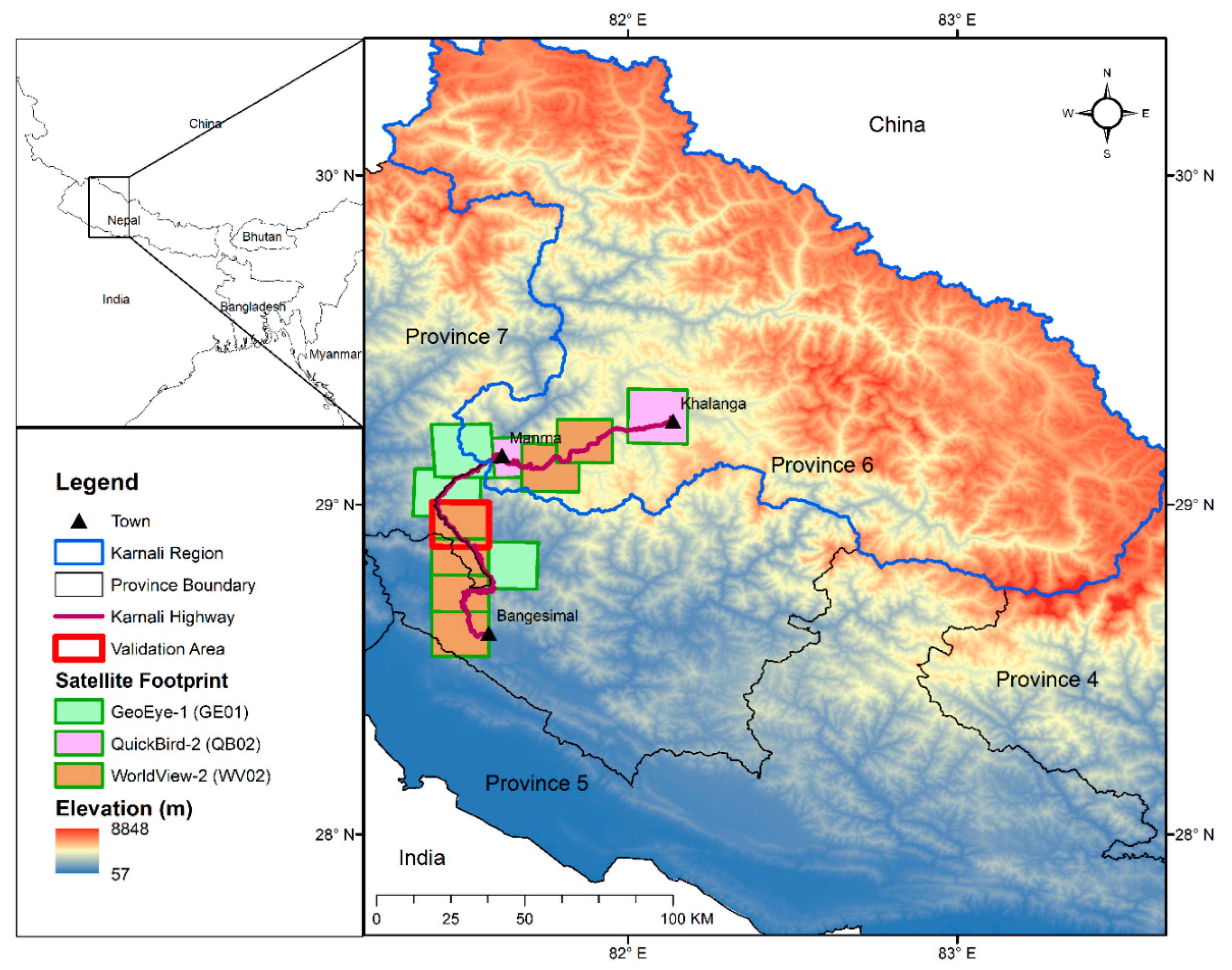
Figure 1. Study area and location of the Karnali highway. The tiles highlight the DigitalGlobe (DG) satellite footprint, with the red box indicating the validation area for the object-based image analysis (OBIA) mapping method. PlanetScope data obtained for 2018, not shown here, covers the same approximate study region as the DG satellite footprint in 22 tiles.
Remotesensing 11 02284 g001
Figure 2. Geologic map of the study area [67] with major thrust faults: Main Frontal Thrust (MFT), Main Boundary Thrust (MBT), Mahabharat Thrust (MT) and Main Central Thrust (MCT).
Remotesensing 11 02284 g002
Figure 3. Landslide explanatory variables. Topographical: (a) elevation; (b) slope; (c) aspect; geological: (d) geology; (e) distance to faults; hydrological: (f) distance to drainage and anthropogenic: (g) land cover; (h) distance to highway.
Remotesensing 11 02284 g003
Figure 4. Workflow chart showing each step taken in object-based image analysis (OBIA) landslide mapping.
Remotesensing 11 02284 g004
Figure 5. (a) Example application of the number of clusters determined using the Elbow method in which bend was calculated at 3 using Elbow point-detection method (normalized difference vegetation index (NDVI) from WV02 image of 8 October 2012); (b) Segmentation using scale parameter 10 and selected likely landslide candidate objects using an NDVI threshold of 0.44 (green polygons).
Remotesensing 11 02284 g005
Figure 6. Subset areas showing the OBIA detected landslide along the Karnali highway obtained from DigitalGlobe (top) and PlanetScope (bottom) for two separate locations.
Remotesensing 11 02284 g006
Figure 7. Location and area of landslides along the Karnali highway for the two mapping periods, 2012 and 2018.
Remotesensing 11 02284 g007
Figure 8. Frequency analysis of the landslide inventory for each explanatory variable: (a) elevation; (b) slope; (c) aspect; (d) geology; (e) distance to fault; (f) distance to drainage; (g) land cover and (h) distance to highway.
Remotesensing 11 02284 g008
Figure 9. Landslide susceptibility map derived from logistic regression with inset plots highlighting two hazardous portions of the Karnali highway.
Remotesensing 11 02284 g009
Figure 10. Receiver operating characteristic (ROC) curve computed from validation sample.
Remotesensing 11 02284 g010
Figure 11. Manually mapped landslides compared with OBIA based landslides.
Remotesensing 11 02284 g011
Table 1. DG imagery used in this study.
SensorAcquisition TimeCloud Cover (%)Off Nadir (degree)Resolution (m)
GE0130 December 2010010.91.65
GE0111 December 2011015.91.65
GE0111 December 2011620.41.65
WV0212 January 2012014.51.85
WV028 October 201209.11.85
WV028 October 20120.68.91.85
WV028 October 201208.71.85
WV028 October 20122.48.51.85
QB0212 October 20120.412.32.4
WV0226 February 201304.21.85
QB0230 May 2013016.52.4
Table 2. Comparison of OBIA and manual landslides based on overlapping landslide area.
True Positive (m2)False Positive (m2)False Negative (m2)Producer Accuracy (%)User Accuracy (%)
110,62561,19276,18159.2264.39
Table 3. Coefficient and test statistics of variables used in logistic regression.
FactorCoefficientStandard Errorz ValuePr(>|z|)
Intercept−6.020.84−7.170.00
Slope1.590.1113.970.00
Aspect0.800.145.550.00
Elevation1.220.177.180.00
Distance to drainage−0.810.73−1.120.26
Geology0.900.118.330.00
Distance to faults0.590.134.450.00
Land cover0.390.152.610.00
Distance to highway0.420.094.880.00
Table 4. Percentage of landslide susceptibility classes in the study area.
Susceptibility%
Very low35.30
Low18.28
Moderate13.45
High14.14
Very high18.83