An Empirical Assessment of the MODIS Land Cover Dynamics and TIMESAT Land Surface Phenology Algorithms

Abstract

Observations of vegetation phenology at regional-to-global scales provide important information regarding seasonal variation in the fluxes of energy, carbon, and water between the biosphere and the atmosphere. Numerous algorithms have been developed to estimate phenological transition dates using time series of remotely sensed spectral vegetation indices. A key challenge, however, is that different algorithms provide inconsistent results. This study provides a comprehensive comparison of start of season (SOS) and end of season (EOS) phenological transition dates estimated from 500 m MODIS data based on two widely used sources of such data: the TIMESAT program and the MODIS Global Land Cover Dynamics (MLCD) product. Specifically, we evaluate the impact of land cover class, criteria used to identify SOS and EOS, and fitting algorithm (local versus global) on the transition dates estimated from time series of MODIS enhanced vegetation index (EVI). Satellite-derived transition dates from each source are compared against each other and against SOS and EOS dates estimated from PhenoCams distributed across the Northeastern United States and Canada. Our results show that TIMESAT and MLCD SOS transition dates are generally highly correlated (r = 0.51-0.97), except in Central Canada where correlation coefficients are as low as 0.25. Relative to SOS, EOS comparison shows lower agreement and higher magnitude of deviations. SOS and EOS dates are impacted by noise arising from snow and cloud contamination, and there is low agreement among results from TIMESAT, the MLCD product, and PhenoCams in vegetation types with low seasonal EVI amplitude or with irregular EVI time series. In deciduous forests, SOS dates from the MLCD product and TIMESAT agree closely with SOS dates from PhenoCams, with correlations as high as 0.76. Overall, our results suggest that TIMESAT is well-suited for local-to-regional scale studies because of its ability to tune algorithm parameters, which makes it more flexible than the MLCD product. At large spatial scales, where local tuning is not feasible, the MLCD product provides a readily available data set based on a globally consistent approach that provides SOS and EOS dates that are comparable to results from TIMESAT.

1. Introduction

Land surface phenology (LSP) observations derived from satellites provide information related to seasonal dynamics in the net ecosystem exchange of carbon [1,2] and surface energy and water balance [3,4] at regional-to-global scales. LSP has also been shown to reflect year-to-year variation in weather and is, therefore, a sensitive indicator of ecosystem response to long-term changes in climate [4,5,6]. Consistent with perturbations expected from climate change, long-term phenology studies have identified widespread trends towards earlier springs and a lengthening of the growing season [1,6,7,8]. In contrast, observed trends towards delayed leaf senescence are less pronounced and are spatially heterogeneous [4,7]. These changes have important implications for ecosystem productivity and function [1,4,9]. Therefore, accurate information regarding the start and end of the growing season is important for monitoring and modeling the impacts of climate change on vegetation and ecosystem processes.

Studies of how growing seasons have changed over the past several decades are supported by both field observations and satellite data. For example, a large number of field studies have explored the phenological response of vegetation to climate change at particular locations or for subsets of species [2,6,10,11]. Satellite-based monitoring of phenology, on the other hand, allows regional-to-global analysis of ecosystem responses to climate change, but does not support species-level modeling and analysis. Early remote sensing-based studies of phenology used coarse spatial resolution imagery from the Advanced Very High Resolution Radiometer-AVHHR, e.g., [12,13,14]. In recent years, however, most studies have exploited image time series at 250 to 500 m spatial resolution derived from NASA’s Moderate Resolution Imaging Spectroradiometer-MODIS, e.g., [8,15,16]. Most recently, a number of studies have begun to use 10–30 m imagery available from Landsat and Sentinel 2, e.g., [17,18,19,20].

A variety of different methods have been used to extract so-called phenological transition dates (i.e., metrics identifying the day of year associated with specific phenophase transitions–see [14]) from time series of spectral vegetation indices such as the normalized difference vegetation index (NDVI). In particular, start of season (SOS) and end of season (EOS) dates are widely estimated from remotely sensed time series using a variety of methods to model observed temporal dynamics, including harmonic analysis [13,21], wavelet decomposition [22], splines [23], and curve fitting [14,15,18,24]. Curve fitting algorithms are the most commonly used, and among them, the asymmetric Gaussian, double logistic, and piecewise logistic functions are widely applied [14,15,20,24,25]. Regardless of the algorithm used, the overall methodology for extracting transition dates generally includes the following steps: assemble satellite vegetation index time series, pre-process (i.e., gap filling, cloud screening, smoothing), identification of valid phenological cycles, function fitting (i.e., splines, double logistic), and lastly either parameter inversion [i.e., 15] or threshold date extraction [i.e., 23]. Hereafter, we refer to the overall implementation of these steps and extraction of transition dates from the TIMESAT program and the MLCD products as phenological methods.

While the data and tools available for estimating LSP have greatly matured over the past three decades, there is no consensus in the community regarding which method is best for a given application, e.g., [26,27]. Specifically, different LSP extraction algorithms and remote sensing data sources generally produce different estimates for start of season (SOS) and end of season (EOS) transition dates [19,28,29,30]. Indeed, the results of [26] demonstrated that different methods applied to the same input data differed in their estimates of SOS over North America by as much as two months. Such differences in phenological transition dates have often been ascribed to differences in the methods used, leading the authors of [26] to conclude that the best way of resolving these discrepancies is to use an ensemble approach. The authors of [31], on the other hand, reconcile the discrepancies by using a novel approach to characterize the phenological cycle based on not only SOS and EOS but on 21 ecologically interpretable metrics characterizing the growing season. Despite the findings of [26] and [31], many users still rely on the MLCD global product or on the TIMESAT software for their applications. Given how widely used MLCD and TIMESAT are, a need exists to analyze the differences in phenological transition dates between these two sources of data, not only for SOS (like [26]) but also for EOS at a higher spatial resolution of 500 m as opposed to 8 km [cf., 26].

In this paper, we present results from a comparison of SOS and EOS dates from the two of the most widely used phenological transition date extraction products developed over the last two decades: (1) TIMESAT, a freely distributed and widely used software package [14]; and (2) the Collections 5 and 6 MODIS Global Land Cover Dynamics (MLCD) product (MCD12Q2), which is the only global operational land surface phenology product currently available to the community [16,23]. The MLCD product provides annual phenological transition dates at global scale that have been used to explore phenological dynamics at regional to continental scales [1,5,32]. The TIMESAT program, on the other hand, allows users to tailor algorithm parameters to specific locations and applications, and has primarily been used to study regional phenological patterns and processes including vegetation dynamics in Ireland [33] and Fennoscandia [34], phenological change in the Sahel [35] and Northern Europe [8], and insect defoliation in birch forests in Sweden [36], among others. These two sources of phenological information are freely available and widely used by the community. However, the similarities and differences in phenological transition dates derived from each source have never been evaluated. The primary goal of this paper is to characterize the nature, magnitude and origins of disagreement between SOS and EOS transition dates provided by TIMESAT against those provided by the MLCD product. To this end, we present a comparison of SOS and EOS dates from TIMESAT and the MLCD product across a range of land cover types and ecological conditions. To evaluate the agreement and differences in SOS and EOS dates from each method, our analysis addresses two main objectives:

• To document the nature and magnitude of random versus systematic errors in LSP metrics from TIMESAT versus those from the MLCD product.
• To explore and explain the causes for the observed differences between LSP metrics from each of these sources.

To perform our analysis, we compared results from the TIMESAT program against the MLCD Collection 5 and 6 products (hereafter referred to as C5 and C6), and also compared results from both products against near-surface remote sensing observations from the PhenoCam network in North America [37].

2. Materials and Methods

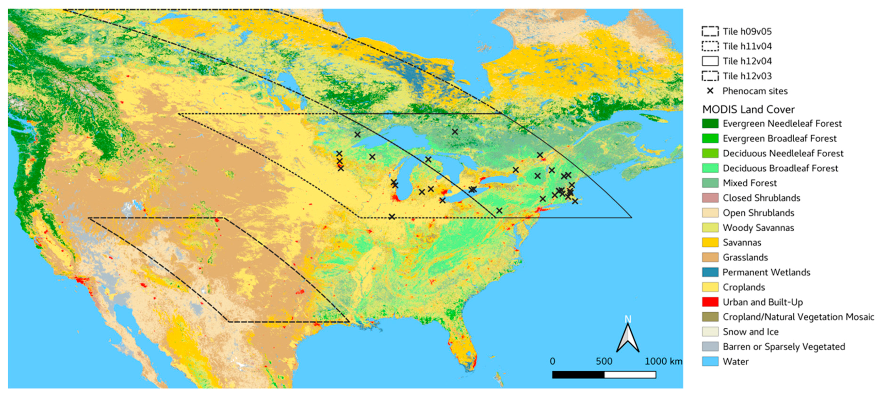
2.1. MODIS NBAR Data and Study Region

Time series of the normalized difference snow index (NDSI) [38] were calculated along with the enhanced vegetation index (EVI) [39] and two-band enhanced vegetation index (EVI2) [40] from MODIS C5 and C6 imagery. To be consistent with the C5 and C6 MLCD, we used EVI for the comparison between TIMESAT and the MLCD C5, and EVI2 for the comparison between TIMESAT and the MLCD C6. All three indices were calculated using Nadir Bidirectional Reflectance Distribution Function (BRDF)-Adjusted Reflectance (NBAR) measurements at 500 m spatial resolution (MCD43A4) from 2003 to 2014 [41,42]. NBAR time series provide surface reflectance measurements that are normalized to a consistent nadir view geometry with solar illumination conditions corresponding to local noon based on BRDF models estimated from multi-angular, cloud-free, atmospherically corrected MODIS surface reflectance measurements [41]. To minimize the influence of negatively biased EVI/EVI2 values, which are primarily caused by clouds, atmospheric constituents and snow contamination, we used NBAR quality assessment data (MCD43A2) to identify low quality and snow-contaminated EVI/EVI2 NBAR data. To select and filter snow contaminated pixels not identified in the C5 NBAR quality assessment flags, we computed NDSI and used a threshold of NDSI > −0.2. Snow contaminated EVI pixels were replaced with the 10% snow-free EVI quantile value at each pixel in each year. The resulting cloud-screened and snow-free MODIS EVI time series were used as input for the TIMESAT program. In the C5 MLCD product, instead of using the 10% snow-free EVI quantile, snow-contaminated values were replaced with the most recent snow-free EVI value at each pixel [15]. For C6 NBAR EVI2 and the C6 MLCD product, snow and ice contaminated values were identified using a similar method where the 10% snow-free EVI quantile was determined, with some exceptions, based on a 3-year window (for details see [23]).

For our analysis, we compared phenological transition dates for SOS and EOS obtained from TIMESAT with corresponding dates from the C5 and C6 MLCD products from 2003 to 2014 for four MODIS tiles in North America (h09v05, h11v04, h12v03, and h12v04) that encompass a range of ecoregions, climate, and land cover types (Figure 1). Hereafter, we refer to these tiles as US Southwest, US Midwest, Central Canada, and US Northeast, respectively. Based on the International Geosphere-Biosphere Programme (IGBP) classification in the C6 MODIS Land Cover Type product (MCD12Q1), we restricted our analysis to the four dominant vegetated land cover classes in each tile, which included croplands, cropland/natural vegetation mosaic, mixed forests, deciduous and broadleaf forests, as well as grasslands and shrublands (Figure 1) [43]. The amplitude and shape of phenological cycles varied by ecosystem and land cover type (for example, see Figure 2c,d). Although in a given 12-month period it is possible for vegetation to have multiple growth cycles (i.e., double-crop agriculture), multiple cycles are relatively rare in our study region. Specifically, across all tiles, fewer than 1.39% of all pixels had more than one phenology cycle per year. For pixels that exhibit multiple cycles, we only examine results for the first cycle in a given year.

2.2. TIMESAT

TIMESAT is a software package for extracting seasonality parameters from time series of remotely sensed vegetation indices [24] (http://web.nateko.lu.se/timesat/timesat.asp). The package was designed for use with high frequency, moderate and coarse spatial resolution imagery from sensors such as MODIS and AVHRR and includes three main methods for fitting smooth time series to remotely sensed data: Savitzky–Golay filtering, and double-logistic and asymmetric Gaussian models (Figure 2a). In TIMESAT, users can select the fitting method used to model time series, detect outliers, and tune the parameters to suit the particular needs of their study and the characteristics of their study site (

Table 1. Input settings for time series processing in TIMESAT for two different fitting methods: double logistic and Savitzky–Golay, as recommended by [44].

Parameter	Short Description	Double Logistic	Savitzky–Golay
Window size	Half window for Savitzky–Golay filtering. Larger values smooth more.	NA	3
Spike method	Based on (1) median filtering and (2) weights from seasonal decomposition by Loess (STL).	1	2
Spike value	Determines the degree of spike removal. Low values remove more spikes.	1.8	NA
Amplitude cutoff value	Series with amplitude smaller than this are not processed.	0.1	0.1
Valid data range	Data outside range is assigned weight 0.	0.01–1.0	0.01–1.0
Season parameter	A value of 1 selected to fit one season per year.	1	1
Number of envelope iterations	Number of iterations for upper envelope adaptation. The range is from 1 to 3.	2	2
Adaptation strength	Strength of the envelope adaptation. The range is from 0 to 10.	2	2

). Here we generated eight sets (4 using EVI time series and 4 using EVI2 time series) of SOS and EOS results from TIMESAT using the double logistic model and the Savitzky–Golay filter fit to MODIS EVI/EVI2 NBAR time series, using the default parameters in TIMESAT for each method (Table 1) [44]. It’s important to note that these two methods have different properties in regard to the way they fit seasonal time series; double logistic functions fit highly generalized seasonal curves that capture the overall seasonal structure while disregarding local variations, whereas Savitzky–Golay filtering smoothly follows within-season variations and therefore captures subtle dynamics during the growing season (Figure 2a). Since Gaussian functions are very similar to the double logistic model, this method was not included in this study. Thus, the tested methods represent the behavior of most algorithms that are commonly used (e.g., harmonic functions are also global, while splines are more local in nature). To determine the day of year (DOY) corresponding to the SOS and EOS at each pixel in each year, we used two thresholds corresponding to 10% and 15% of the seasonal amplitude of EVI in spring and fall (Figure 2b). These thresholds were selected based on the C5 and C6 MLCD thresholds so that the phenological transition dates of the MLCD products and those derived from the TIMESAT approaches would be comparable.

2.3. MODIS Land Cover Dynamics

We used satellite-based observations of LSP from the MODIS C5 and C6 MLCD products. In C5, vegetation growth cycles were characterized using four transition dates estimated from time series of C5 MODIS NBAR EVI at 500 m spatial resolution [15,16]. To do this, the C5 MLCD algorithm fit piecewise logistic functions to EVI time series at each pixel, and used maxima in the rate of change in curvature to determine the DOY corresponding to key phenological transition dates: (1) the onset of EVI increase (i.e., SOS), (2) the onset of EVI maximum (maximum canopy development), (3) the onset of EVI decrease (senescence), and (4) the onset of EVI minimum (i.e., EOS). In the C6 MLCD product, outliers were removed and smooth EVI2 time series were generated in a single step using penalized cubic splines [23]. In this approach, the timing of (1) greenup onset and dormancy onset, (2) mid-greenup and mid-senescence, (3) maturity onset and senescence onset were determined as the DOY when the splined EVI2 time series first/last crossed 15%, 50%, and 90% of seasonal amplitude, respectively.

2.4. PhenoCam Sites and Data

Phenological transition dates from TIMESAT and the MLCD products were compared against transition dates estimated from time series of vegetation canopy greenness measurements derived from PhenoCam imagery. PhenoCams are digital webcams mounted above the vegetation canopy that acquire data at high-repeat frequencies (i.e., 30-min to daily intervals; http://explore.phenocam.us/) [37]. Previous studies have demonstrated the ability of PhenoCam observations to quantitatively monitor the seasonal development of both deciduous and conifer canopies [5,45,46]. In this study, we used SOS and EOS dates from 47 PhenoCams from the PheoCam Dataset v1.0 (Table S1) from 2006 to 2014 that overlapped with our study area [37], totaling 177 site-years for SOS and 192 site-years for EOS. PhenoCam SOS and EOS dates were estimated from green chromatic coordinate (GCC) time series extracted from a manually delineated region of interest at each site. SOS and EOS dates were estimated using three-day GCC data; first seasonal amplitude of GCC was calculated and then dates were identified when the spline exceeded 10% of the amplitude at each site [37].

2.5. Comparison of Land Surface Phenology Metrics

In each MODIS tile, we selected a random sample of 500 pixels from each of the four most common land cover classes. To compare phenological transition dates derived from the four different phenology extraction methods (TIMESAT Savitzky–Golay, TIMESAT double logistic, MODIS C5 and MODIS C6) we pooled all 500 pixels together and computed the root mean square error (RMSE), bias, and correlation coefficients for SOS and EOS transition dates from MLCD versus TIMESAT. For each comparison, we report the correlation coefficient (R) and the associated statistical significance (p < 0.05). The bias (in days) was calculated relative to the MLCD products, so a negative bias indicates that the MLCD transition dates were later than TIMESAT transition dates. The analysis of transition dates derived from the different fitting methods was stratified by region (US Southwest, US Midwest, US Northeast and Central Canada), by phenological transition dates (SOS and EOS), and by land cover class (Agricultural Mosaic, Croplands, Deciduous Forest, Evergreen Forest, Mixed Forest, Grasslands, Open Shrublands, Savannas, and Woody Savannas). Finally, SOS and EOS dates from the C5 and C6 MLCD products and TIMESAT were compared with corresponding transition dates from near-surface PhenoCam imagery.

3. Results

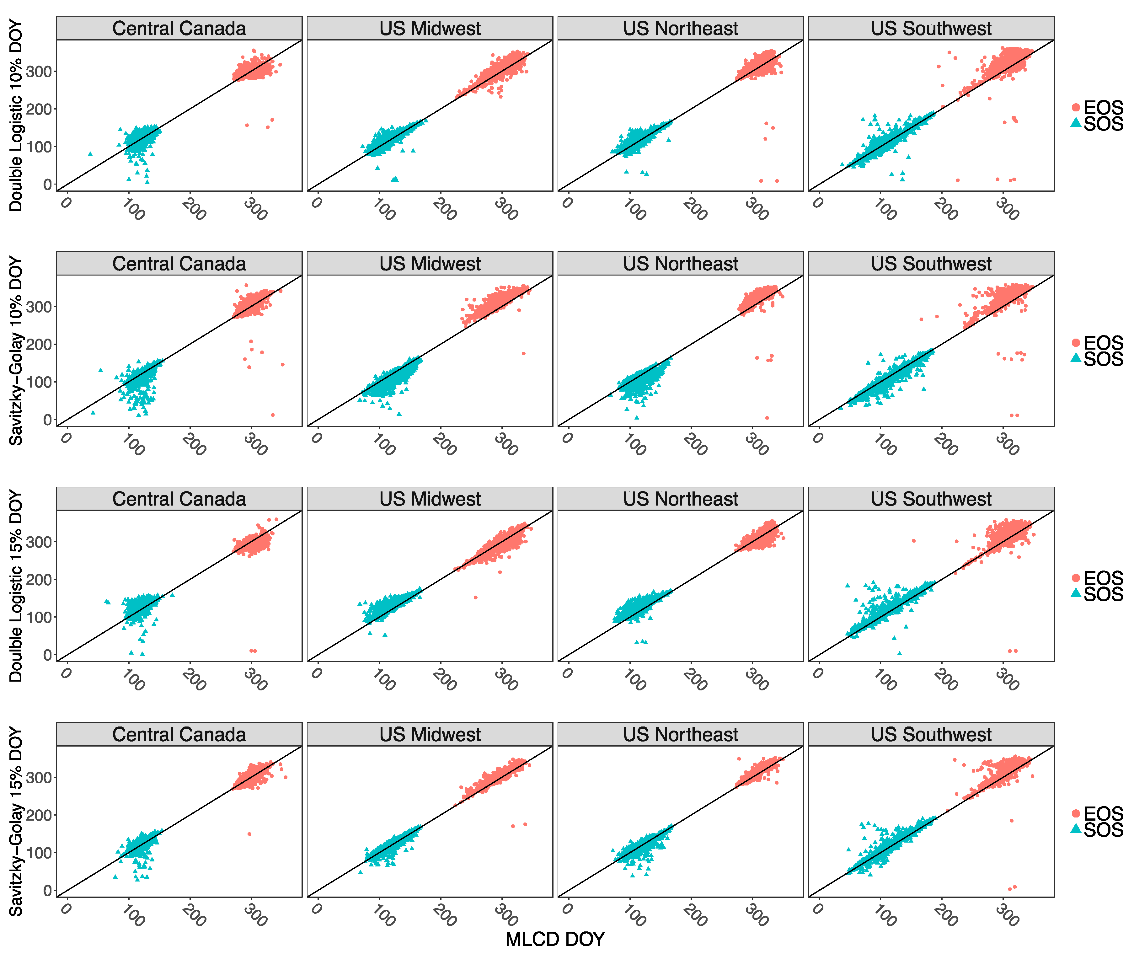
3.1. Comparison among Median SOS and EOS Transition Dates

We characterized the nature and magnitude of variability in phenological metrics across different fitting methods at interannual time scales from 2003 to 2014. Figure S4 presents the distribution of phenological transitions for each of the four MODIS tiles and five fitting methods. Across regions, the estimated median phenological transition from Savitzky–Golay using a 10% threshold is always the earliest during SOS, whereas the estimated median SOS from the double logistic using a 15% threshold is always the latest during SOS (Figure S4). The variability in median phenological transition dates is highest in the US Southwest.

In addition to characterizing the variability in median phenological transition dates, we also evaluated the agreement between SOS and EOS dates estimated by the TIMESAT program against corresponding dates from the C5 and C6 MLCD products (Figure 3, Table S2, Table S3). Specifically, Figure 3 shows a statistical summary that compares SOS dates from the C5 and C6 MLCD products against TIMESAT based on 10% and 15% thresholds of the seasonal amplitude using the Savitzky–Golay filter and double logistic models. SOS and EOS derived from TIMESAT exhibited generally (but not uniformly) strong agreement with the C5 and C6 MLCD products (Figure 3, Figure S1). The correlation coefficients between TIMESAT versus C6 MLCD were higher and the RMSE was lower during SOS (average r = 0.79; average RMSE = 9.10 days) compared to EOS (average r = 0.70; average RMSE = 11.9 days) (Figure 3, Figure S1). SOS RMSEs were generally consistent across regions with values averaging about 8 days with C6 (10 days with C5) in the US Midwest and US Northeast and 10 days with C6 (13 days with C5) in US Southwest and Central Canada (Figure 3).

Overall, we found that results were quite consistent across satellite-based methods, with some explainable discrepancies in Central Canada. While SOS correlations were generally good, with correlation coefficients ranging from 0.51 to 0.97 across methods and regions, correlations in Central Canada were as low as 0.25 (Figure 3, Table S2, Table S3). In general, the Savitzky–Golay fitting method at 10% amplitude showed lower agreement and higher systematic bias with the C5 and C6 MLCD products compared to other TIMESAT methods (Figure 3, Table S2, Table S3). Conversely, in Central Canada agreement was higher between results from the MLCD products and TIMESAT using Savitzky–Golay filtering. While there was notable spread around the 1:1 line for SOS in Central Canada, during EOS there was less variability in the transition dates (Figure 4). To explore these discrepancies further, we investigated clusters with very early EOS (DOY ≤ 20) in TIMESAT, which are not present in MLCD, and determined that these differences were associated with TIMESAT EOS transition dates that were estimated to have occurred in the first few days of the subsequent year (Figure 4). Overall, correlations between TIMESAT and MLCD phenological transition dates were consistently higher (RMSE consistently lower) with C6 compared to C5 (Figure 3). The most notable improvement in agreement between results from TIMESAT and C6 MLCD relative to C5 MLCD was in problematic areas such as Central Canada and the US Southwest where the spread around the 1:1 line decreased substantially with C6 (Figure S2). We postulate that the largest disagreements among methods are caused by differences in snow screening, especially in Central Canada, where differences in phenological transition dates among methods were highest (Figure 4).

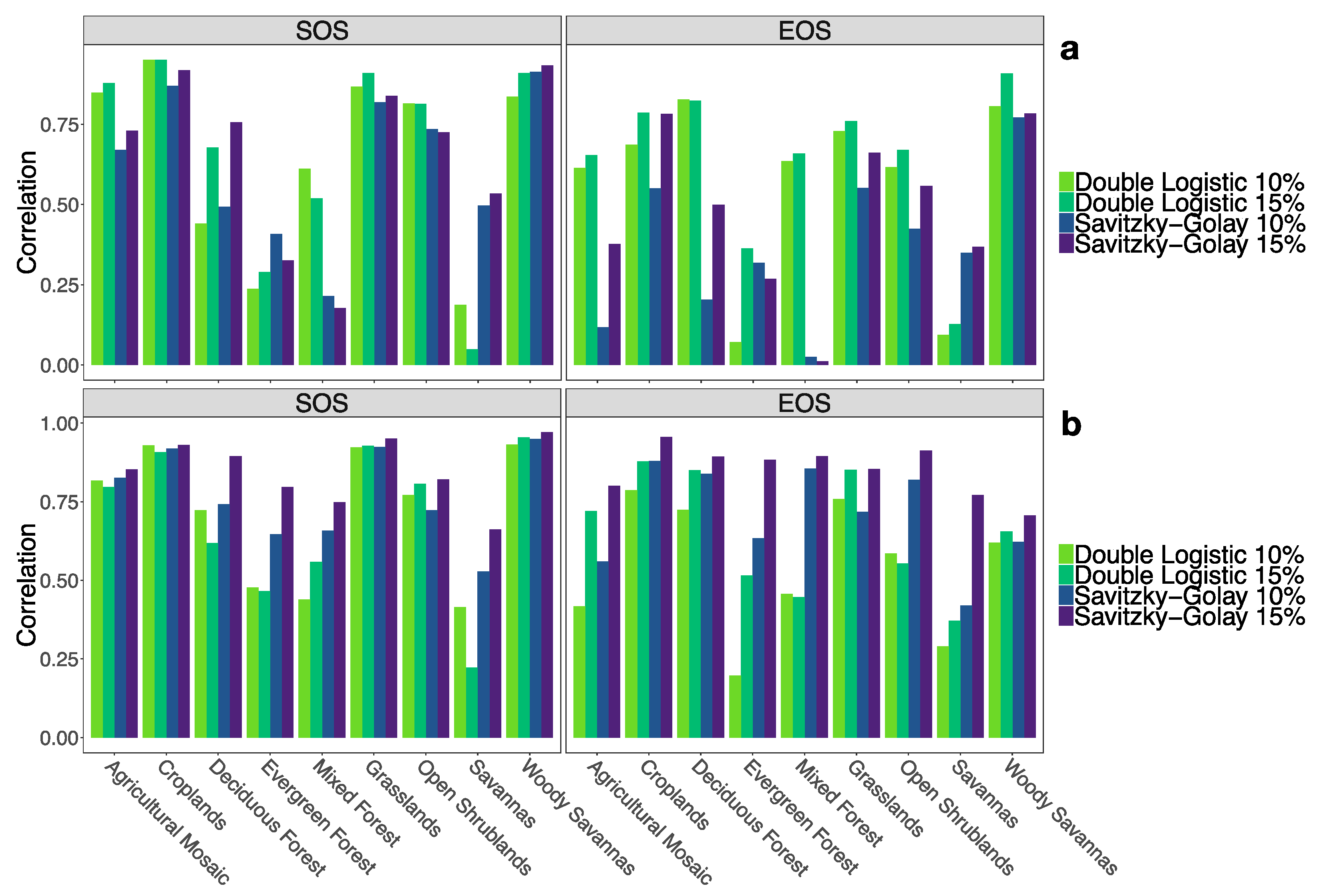
3.2. Comparison by Land Cover Class

To further investigate patterns of agreement and disagreement among methods, we stratified our analysis by land cover class. Figure 5 shows that the largest discrepancies in the timing of SOS and EOS between results from TIMESAT and the MLCD products were associated with land cover types that traditionally present the biggest challenges for retrieval of land surface phenology: evergreen forests and mixed land cover types including mixed forests and savannas (Figure 2c,d, Figure 5). Further, agreement among methods was higher with C6 MLCD compared to C5 MLCD for almost all land cover classes during both SOS and EOS. For example, agreement between results from TIMESAT and C5 MLCD in evergreen forests was low across all methods during both SOS (average r = 0.31) and EOS (average r = 0.25) (Figure 5a). (This is the average of all methods shown in Figure 5.) However, for C6 MLCD agreement in evergreen forest was much higher, with an average correlation of 0.60 during SOS and an average correlation of 0.56 for EOS (Figure 5b). More generally, agreement between SOS and EOS dates from TIMESAT Savitzky–Golay versus the C6 MLCD product improved for all problematic classes, with correlation coefficients above 0.50 in most cases (Figure 5). Despite overall improvement, agreement between TIMESAT double logistic and C6 MLCD remained low to moderate for evergreen forests, mixed forests, and savannas.

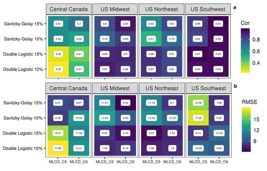
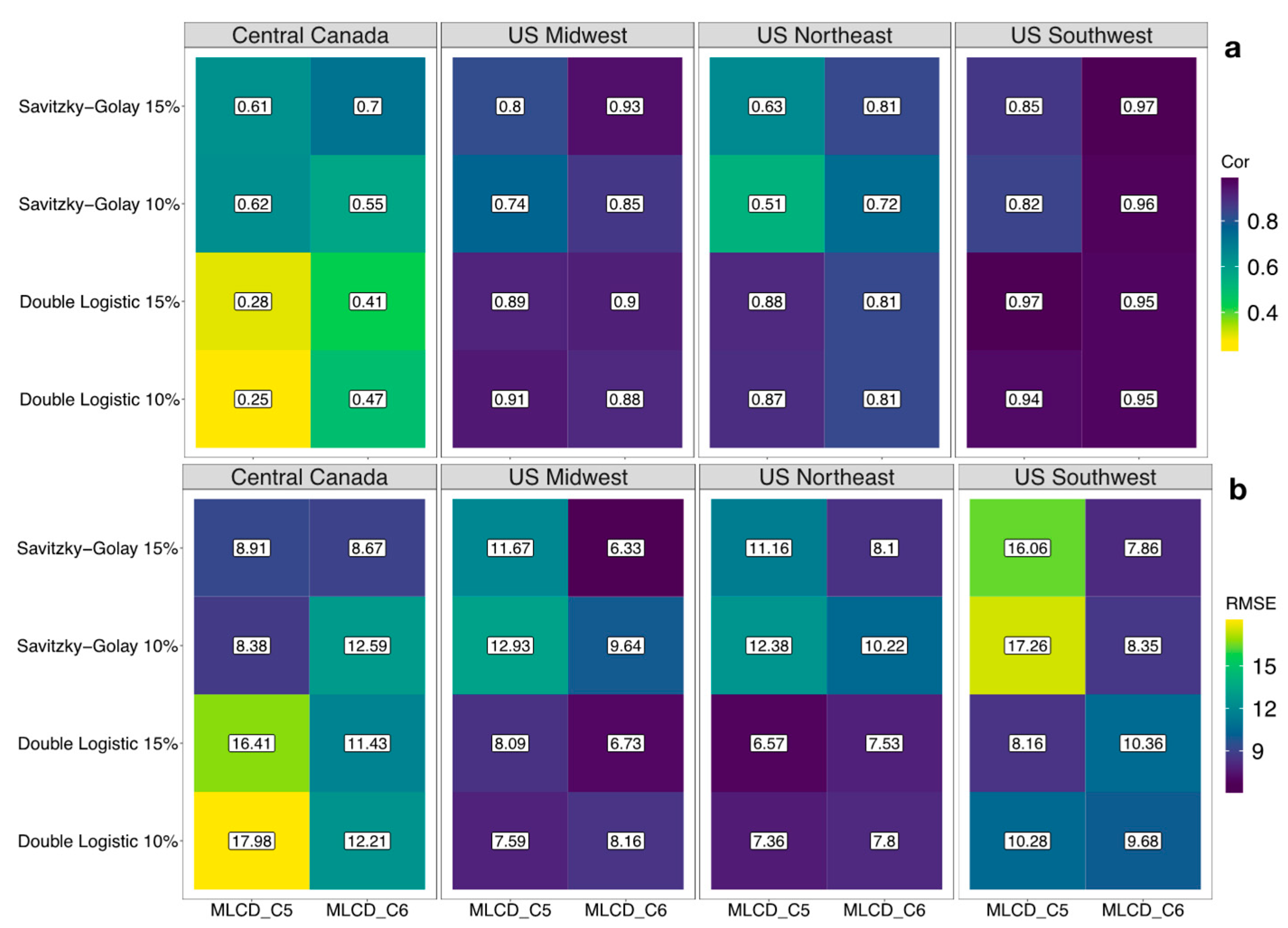
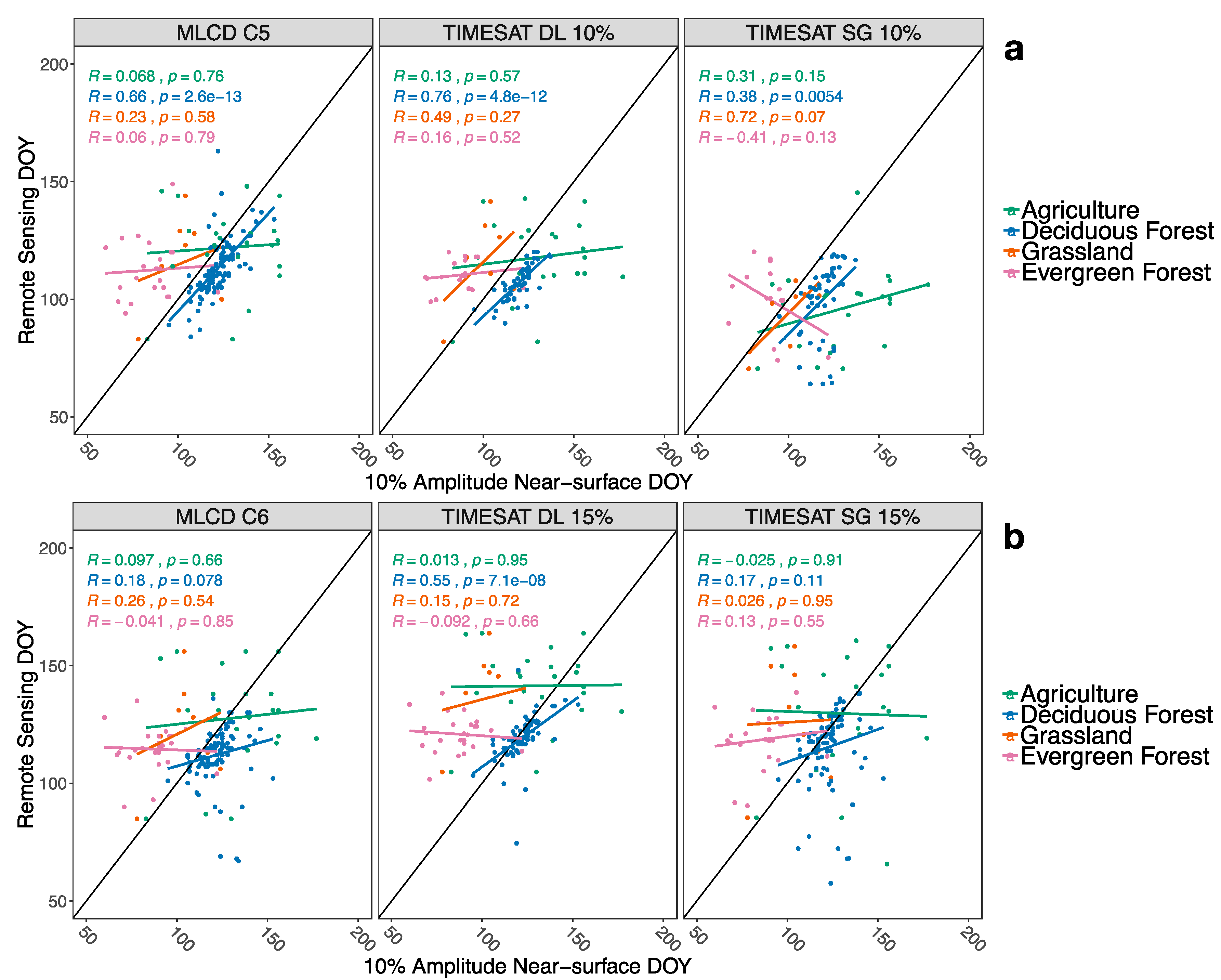
3.3. Comparison between Result from PhenoCam and MODIS

Agreement between phenological dates derived from MODIS-based methods and PhenoCam depends on land cover type and heterogeneity surrounding PhenoCam sites [37]. Consistent with this, results from our analysis show large discrepancies between SOS and EOS dates from PhenoCam versus those from MODIS (MLCD and TIMESAT) in agricultural and evergreen sites with correlations of 0.31 or less (Figure 6, Figure S3). The agricultural PhenoCam sites in this study tended to be located in heterogeneous landscapes (e.g., Kellog Biological Station) that include a matrix of crops and natural land cover [37]. Similarly, there was poor to moderate agreement between PhenoCam- and MODIS-derived SOS and EOS dates in grasslands, again ostensibly because of site heterogeneity (e.g., University of Illinois Energy Farm Restored Prairie). Agreement in deciduous forests, on the other hand, was moderate with correlations of ~0.45 for SOS and ~0.50 for EOS (Figure 6, Figure S3). For deciduous forests, TIMESAT double logistic 10% estimates had the strongest agreement, with PhenoCam-derived estimates of SOS (r = 0.76, Figure 6a). Overall agreement between phenological transition dates from PhenoCam versus the MLCD products was stronger for C5 compared to C6, most likely because the C6 MLCD algorithm used 15% of EVI2 amplitude to determine transition dates, which does not match the 10% of amplitude threshold used to estimate SOS and EOS from PhenoCam GCC data. However, C5 MLCD dates showed an average systematic bias of 10 days early and 7 days late for SOS and EOS, respectively, compared to PhenoCam estimates (Figure 6, Figure S3). This is consistent with other studies showing that MODIS products predict SOS early relative to field observations for a variety of reasons, most notably the impact of snowmelt and understory vegetation, for which leaf emergence tends to precede the tree canopy in forests [37].

4. Discussion

SOS and EOS values from TIMESAT and the MLCD products are directly comparable because they are derived using the same EVI/EVI2 time series calculated from MODIS NBAR data. Hence, observed discrepancies in SOS and EOS dates were caused by two main sources: (1) differences in the underlying method used to estimate phenological transition dates, and (2) method-specific snow screening and treatment of missing data. Because LSP results are sensitive to methods used to pre-process input data, there is continued need in the phenology community to understand how to best identify noise and gap-fill time series prior to applying LSP methods [26,47,48]. Based on the results presented here, we recommend that TIMESAT users employ vegetation indices that are specifically designed for use in areas with seasonal snow cover, e.g., [49,50], or use the normalized difference snow index (NDSI) index in addition to the MODIS quality flags to screen data for snow and cloud contaminated EVI values [23,43].

4.1. Differences in Fitting Methods and Thresholds Used to Identify Transition Dates

Our results do not identify a single method that is universally preferred or superior to the other methods examined. However, our results do suggest several key strengths and weaknesses of each method. Since no one method is optimal, users should consider the ultimate objective of their study as well as the vegetation cover in their region of interest. For local-to-regional scale studies, TIMESAT has substantial advantages because it allows users to specify different fitting methods and thresholds based on land cover and LSP dynamics. At the same time, users should be aware that (like with all methods) LSP metrics estimated from TIMESAT are dependent on the quality of the input data. Results from regions with frequent snow or clouds (e.g., Central Canada), or low seasonal EVI amplitude (e.g., US Southwest) have lower quality relative to results from regions with strong seasonality that have fewer sources of noise (e.g., US Northeast) (Figure 3, Figure 5). In this context, it is important to understand that differences in tuning parameters (e.g., using 10% versus 15% of seasonal amplitude as a threshold to determine transition dates) can produce quite different results (Figure 3, Table S2, Table S3). In TIMESAT, selection of fitting methods for the time series and land cover-specific tuning of model parameters is most productive when users are knowledgeable of the particular characteristics of their study site and have reliable ground data to evaluate their results. The advantage of the MLCD product, on the other hand, is that it provides global time series of land surface phenology data that are produced operationally and consistently across all locations in a way that is not feasible using the TIMESAT program.

Overall, we found that results were quite consistent across satellite-based methods, land cover classes, and time of year. Specifically, comparison of SOS and EOS dates among methods and regions indicates that the TIMESAT double logistic model has higher overall agreement with the C5 MLCD product compared to Savitzky–Golay (Figure 3, Table S2, Table S3), which is consistent with conclusions from previous studies by [14,24,25,51]. The similar functional form of the double logistic function used by TIMESAT and the piecewise logistic of the C5 MLCD product explains this agreement. Low agreement between MLCD and TIMESAT double logistic in Central Canada is due to double logistic fitting method producing spurious results due to low EVI values prior to SOS (Figure S5). The shape of the curve leads to an early estimate of SOS due to the inflexible form of the double logistic relative to the local fitting capability of Savitzky–Golay. In deciduous forests, results from TIMESAT using the double logistic function and the C5 MLCD product show good agreement with results from PhenoCam data, which supports the conclusion that these algorithms provide a good representation of vegetation phenology in ecoregions with strong seasonality in EVI/EVI2 (Figure 6). Similarly, high agreement between SOS and EOS dates from the C6 MLCD and TIMESAT based on Savitzky–Golay filtering is explained by the fact that both functions employ local fitting methods to model EVI2 time series. Relative to collection 5, improvements in time series density and input data quality in MODIS collection 6 also contribute to overall better agreement of the C6 MLCD with results from TIMESAT. In addition, both the C6 MLCD product and TIMESAT use thresholds of seasonal amplitude to determine SOS and EOS dates [14,23], while the C5 MLCD product uses an approach based on the rate of curvature in fitted logistic functions.

4.2. Differences in Land Cover

Stratification by land cover type reveals that both the choice of criteria used to determine phenological transition dates (e.g., 10% vs. 15% of EVI amplitude) and biogeographical regions (i.e., Central Canada) influence agreement across methods. For both SOS and EOS, agreement between results from TIMESAT and the MLCD product is higher with C6 MODIS (Figure 5b) and in particular the agreement between C6 MLCD and TIMESAT Savitzky–Golay is higher compared to results from the double logistic. However, there is a poor agreement between results from TIMESAT and the MLCD products in vegetation types with low seasonal EVI amplitude (i.e., evergreen forests and savannas) [25,52] (Figure 2c,d). When the land cover in a pixel has low seasonal amplitude in EVI/EVI2, subtle differences in the pre-processing of the data and the phenology extraction methods applied can result in different estimates of SOS and EOS. As a result, savannas located in US Southwest showed only low to moderate agreement across methods and high variation in SOS (Figure S4). Similarly, agreement was consistently lower for evergreen forests, where phenological amplitude is relatively low, time series are irregular, and it’s challenging to detect subtle changes in EVI/EVI2 (Figure 2c). Lastly, mixed forests also showed lower overall agreement because weaker seasonality in vegetation indices make it hard to unambiguously identify the maximum and minimum EVI/EVI2 [52]. In contrast, agreement among results from the different methods is high in regions that are relatively homogeneous with vegetation types that exhibit pronounced EVI/EVI2 seasonal amplitude (i.e., deciduous forests and croplands) (Figure 3, Figure 4). The inability of SOS and EOS metrics to effectively capture the phenology dynamics of these land cover classes could perhaps be ameliorated by using a muti-dimensional approach that captures more metrics that characterize the phenological cycle and explicitly includes variance [31]. However, this type of analysis is beyond the scope of this work.

4.3. Comparison with Near-Surface PhenoCam Data

Despite moderate to high agreement between satellite-based and near-surface SOS and EOS dates in deciduous forests, phenological transition dates in other land cover types show relatively low agreement (Figure 6, Figure S3). Specifically, for deciduous forests, the TIMESAT double logistic approach has the highest agreement with PhenoCam results compared to the MLCD product and TIMESAT Savitzky–Golay approach. For all other land cover types, the agreement is usually low to moderate and no satellite-based method clearly outperforms the rest. This suggests that for land cover types where agreement between satellite-based and near-surface phenological transition dates is moderate to high, TIMESAT based on a double logistic model is able to capture on the ground phenology dynamics better than MLCD. However, it’s important to note that results from comparisons between transition dates derived from PhenoCam and the MLCD product or TIMESAT depend strongly on how representative the PhenoCam camera field of view is of the landscape-based field of view recorded by MODIS. Indeed, the relatively low agreement outside of deciduous forests highlights the primary limitation of coarse resolution imagery for mapping and monitoring LSP in heterogeneous landscapes [5,37,46].

Further, because the geographic distribution of PhenoCam sites included in our analysis was restricted to the Central and Northeastern United States, our study does not provide a comprehensive characterization of error in satellite measurements of phenology relative to field observations. Lastly, PhenoCams may not compare well with MODIS because of two limiting factors: (1) GCC utilizes information only from visible channels, whereas EVI/EVI2 values include information from MODIS’ near-infrared band, which responds strongly to canopy dynamics; and (2) PhenoCams generally use oblique view angles, which can cause strong directional effects that can bias SOS and EOS estimates relative to values derived from nadir viewing sensors [53]. Generally, robust assessment of LSP metrics from satellites requires consistent and long-term observations of phenology on the ground at spatial scales that are commensurate with the measurements and field of view provided by space-borne remote sensing instruments. Future studies would benefit from additional ground-based measurements that complement PhenoCam observations, including flux towers [54], professional on-the-ground observers [34], and field spectral measurements [27].

5. Conclusions

Phenological observations derived from satellites at seasonal and interannual time scales provide information related to biosphere-atmosphere exchanges of carbon, energy, and water at regional to global scales. This study provides a comprehensive comparison of start of season and end of season phenology for the two most widely used satellite-based LSP sources: TIMESAT and the MODIS Global Land Cover Dynamics (MLCD) product. Our results demonstrate that there is higher agreement among methods during SOS compared to EOS, and that results from TIMESAT show higher agreement with C6 MLCD results compared to C5 MLCD. While our results do not identify a method that is universally best, we identify several key strengths and weaknesses of the different methods. For local-to-regional studies that cover diverse vegetation types and physical environments and for users who are knowledgeable of the particular characteristics of their study site, TIMESAT has substantial advantages because it allows users to specify different fitting methods and thresholds based on land cover class. However, because of noise in time series of satellite data, especially in northern regions, we recommend that TIMESAT users carefully filter input data for snow contamination using the normalized difference snow index (NDSI) in addition to using the quality flags for MODIS products. For regional-to-global studies, we recommend the use of the MLCD product as it provides high quality, consistent and reliable observations at large spatial scales.

References

1. Keenan, T.F.; Gray, J.; Friedl, M.A.; Toomey, M.; Bohrer, G.; Hollinger, D.Y.; Munger, J.W.; O’Keefe, J.; Schmid, H.P.; Wing, I.S.; et al. Net Carbon Uptake Has Increased through Warming-Induced Changes in Temperate Forest Phenology. Nat. Clim. Chang. 2014, 4, 598–604. [Google Scholar] [CrossRef]
2. Migliavacca, M.; Sonnentag, O.; Keenan, T.F.; Cescatti, A.; O’Keefe, J.; Richardson, A.D. On the Uncertainty of Phenological Responses to Climate Change, and Implications for a Terrestrial Biosphere Model. Biogeosciences 2012, 9, 2063–2083. [Google Scholar] [CrossRef]
3. Baldocchi, D.D.; Xu, L.; Kiang, N. How Plant Functional-Type, Weather, Seasonal Drought, and Soil Physical Properties Alter Water and Energy Fluxes of an Oak–Grass Savanna and an Annual Grassland. Agric. For. Meteorol. 2004, 123, 13–39. [Google Scholar] [CrossRef]
4. Richardson, A.D.; Keenan, T.F.; Migliavacca, M.; Ryu, Y.; Sonnentag, O.; Toomey, M. Climate Change, Phenology, and Phenological Control of Vegetation Feedbacks to the Climate System. Agric. For. Meteorol. 2013, 169, 156–173. [Google Scholar] [CrossRef]
5. Hufkens, K.; Friedl, M.; Sonnentag, O.; Braswell, B.H.; Milliman, T.; Richardson, A.D. Linking Near-Surface and Satellite Remote Sensing Measurements of Deciduous Broadleaf Forest Phenology. Remote Sens. Environ. 2012, 117, 307–321. [Google Scholar] [CrossRef]
6. Menzel, A.; Sparks, T.H.; Estrella, N.; Koch, E.; Aasa, A.; Ahas, R.; Alm-Kübler, K.; Bissolli, P.; Braslavská, O.; Briede, A.; et al. European Phenological Response to Climate Change Matches the Warming Pattern. Glob. Chang. Biol. 2006, 12, 1969–1976. [Google Scholar] [CrossRef]
7. Walther, G.-R.; Post, E.; Convey, P.; Menzel, A.; Parmesan, C.; Beebee, T.J.; Fromentin, J.-M.; Hoegh-Guldberg, O.; Bairlein, F. Ecological Responses to Recent Climate Change. Nature 2002, 416, 389–395. [Google Scholar] [CrossRef] [PubMed]
8. Jin, H.; Jönsson, A.M.; Olsson, C.; Lindström, J.; Jönsson, P.; Eklundh, L. New Satellite-Based Estimates Show Significant Trends in Spring Phenology and Complex Sensitivities to Temperature and Precipitation at Northern European Latitudes. Int. J. Biometeorol. 2019, 63, 763–775. [Google Scholar] [CrossRef]
9. Penuelas, J.; Rutishauser, T.; Filella, I. Phenology Feedbacks on Climate Change. Science 2009, 324, 887–888. [Google Scholar] [CrossRef] [Green Version]
10. Parmesan, C.; Yohe, G. A Globally Coherent Fingerprint of Climate Change Impacts across Natural Systems. Nature 2003, 421, 37–42. [Google Scholar] [CrossRef]
11. Richardson, A.D.; Bailey, A.S.; Denny, E.G.; Martin, C.W.; O’Keefe, J. Phenology of a Northern Hardwood Forest Canopy. Glob. Chang. Biol. 2006, 12, 1174–1188. [Google Scholar] [CrossRef]
12. Reed, B.C.; Brown, J.F.; VanderZee, D.; Loveland, T.R.; Merchant, J.W.; Ohlen, D.O. Measuring Phenological Variability from Satellite Imagery. J. Veg. Sci. 1994, 5, 703–714. [Google Scholar] [CrossRef]
13. Stöckli, R.; Vidale, P.L. European Plant Phenology and Climate as Seen in a 20-Year AVHRR Land-Surface Parameter Dataset. Int. J. Remote Sens. 2004, 25, 3303–3330. [Google Scholar] [CrossRef]
14. Jönsson, P.; Eklundh, L. Seasonality Extraction by Function Fitting to Time-Series of Satellite Sensor Data. IEEE Trans. Geosci. Remote Sens. 2002, 40, 1824–1832. [Google Scholar] [CrossRef]
15. Zhang, X.; Friedl, M.A.; Schaaf, C.B.; Strahler, A.H.; Hodges, J.C.; Gao, F.; Reed, B.C.; Huete, A. Monitoring Vegetation Phenology Using MODIS. Remote Sens. Environ. 2003, 84, 471–475. [Google Scholar] [CrossRef]
16. Ganguly, S.; Friedl, M.A.; Tan, B.; Zhang, X.; Verma, M. Land Surface Phenology from MODIS: Characterization of the Collection 5 Global Land Cover Dynamics Product. Remote Sens. Environ. 2010, 114, 1805–1816. [Google Scholar] [CrossRef]
17. Fisher, J.; Mustard, J.; Vadeboncoeur, M. Green Leaf Phenology at Landsat Resolution: Scaling from the Field to the Satellite. Remote Sens. Environ. 2006, 100, 265–279. [Google Scholar] [CrossRef]
18. Melaas, E.K.; Friedl, M.A.; Zhu, Z. Detecting Interannual Variation in Deciduous Broadleaf Forest Phenology Using Landsat TM/ETM+ Data. Remote Sens. Environ. 2013, 132, 176–185. [Google Scholar] [CrossRef]
19. Melaas, E.K.; Sulla-Menashe, D.; Friedl, M.A. Multidecadal Changes and Interannual Variation in Springtime Phenology of North American Temperate and Boreal Deciduous Forests. Geophys. Res. Lett. 2018, 45, 2679–2687. [Google Scholar] [CrossRef]
20. Jönsson, P.; Cai, Z.; Melaas, E.; Friedl, M.; Eklundh, L. A Method for Robust Estimation of Vegetation Seasonality from Landsat and Sentinel-2 Time Series Data. Remote Sens. 2018, 10, 635. [Google Scholar] [CrossRef]
21. Jakubauskas, M.E.; Legates, D.R.; Kastens, J.H. Harmonic analysis of time-series AVHRR NDVI data. Photogramm. Eng. Remote Sens. 2001, 67, 461–470. [Google Scholar]
22. Sakamoto, T.; Yokozawa, M.; Toritani, H.; Shibayama, M.; Ishitsuka, N.; Ohno, H. A Crop Phenology Detection Method Using Time-Series MODIS Data. Remote Sens. Environ. 2005, 96, 366–374. [Google Scholar] [CrossRef]
23. Gray, J.M.; Melaas, E.K.; Sulla-Menashe, D.; Moon, M.; Friedl, M.A. Global Land Surface Phenology from MODIS: Collection 6 Products. Remote Sens. Environ. 2019. in Preparation. [Google Scholar]
24. Jönsson, P.; Eklundh, L. TIMESAT—A Program for Analyzing Time-Series of Satellite Sensor Data. Comput. Geosci. 2004, 30, 833–845. [Google Scholar] [CrossRef]
25. Beck, P.S.A.; Atzberger, C.; Høgda, K.A.; Johansen, B.; Skidmore, A.K. Improved Monitoring of Vegetation Dynamics at Very High Latitudes: A New Method Using MODIS NDVI. Remote Sens. Environ. 2006, 100, 321–334. [Google Scholar] [CrossRef]
26. White, M.A.; de BEURS, K.M.; Didan, K.; Inouye, D.W.; Richardson, A.D.; Jensen, O.P.; O’Keefe, J.; Zhang, G.; Nemani, R.R.; van LEEUWEN, W.J.D.; et al. Intercomparison, Interpretation, and Assessment of Spring Phenology in North America Estimated from Remote Sensing for 1982-2006. Glob. Chang. Biol. 2009, 15, 2335–2359. [Google Scholar] [CrossRef]
27. Cai, Z.Z.; Jönsson, P.; Jin, H.X.; Eklundh, L. Performance of Smoothing Methods for Reconstructing NDVI Time-Series and Estimating Vegetation Phenology from MODIS Data. Remote Sens. 2017, 9, 1271. [Google Scholar] [CrossRef]
28. Piao, S.; Friedlingstein, P.; Ciais, P.; Viovy, N.; Demarty, J. Growing Season Extension and Its Impact on Terrestrial Carbon Cycle in the Northern Hemisphere over the Past 2 Decades: PHENOLOGY AND CARBON CYCLE IN NH. Glob. Biogeochem. Cycles 2007, 21. [Google Scholar] [CrossRef]
29. Zhang, X.; Tarpley, D.; Sullivan, J.T. Diverse Responses of Vegetation Phenology to a Warming Climate. Geophys. Res. Lett. 2007, 34, 1–5. [Google Scholar] [CrossRef]
30. Jeong, S.-J.; Ho, C.-H.; Gim, H.-J.; Brown, M.E. Phenology Shifts at Start vs. End of Growing Season in Temperate Vegetation over the Northern Hemisphere for the Period 1982–2008: PHENOLOGY SHIFTS AT START VS. END OF GROWING SEASON. Glob. Chang. Biol. 2011, 17, 2385–2399. [Google Scholar] [CrossRef]
31. Buitenwerf, R.; Rose, L.; Higgins, S.I. Three Decades of Multi-Dimensional Change in Global Leaf Phenology. Nat. Clim. Chang. 2015, 5, 364–368. [Google Scholar] [CrossRef]
32. Friedl, M.A.; Gray, J.M.; Melaas, E.K.; Richardson, A.D.; Hufkens, K.; Keenan, T.F.; Bailey, A.; O’Keefe, J. A Tale of Two Springs: Using Recent Climate Anomalies to Characterize the Sensitivity of Temperate Forest Phenology to Climate Change. Environ. Res. Lett. 2014, 9, 054006. [Google Scholar] [CrossRef]
33. O’Connor, B.; Dwyer, E.; Cawkwell, F.; Eklundh, L. Spatio-Temporal Patterns in Vegetation Start of Season across the Island of Ireland Using the MERIS Global Vegetation Index. ISPRS J. Photogramm. Remote Sens. 2012, 68, 79–94. [Google Scholar] [CrossRef]
34. Jin, H.; Jönsson, A.M.; Bolmgren, K.; Langvall, O.; Eklundh, L. Disentangling Remotely-Sensed Plant Phenology and Snow Seasonality at Northern Europe Using MODIS and the Plant Phenology Index. Remote Sens. Environ. 2017, 198, 203–212. [Google Scholar] [CrossRef]
35. Heumann, B.W.; Seaquist, J.W.; Eklundh, L.; Jönsson, P. AVHRR Derived Phenological Change in the Sahel and Soudan, Africa, 1982–2005. Remote Sens. Environ. 2007, 108, 385–392. [Google Scholar] [CrossRef]
36. Olsson, P.-O.; Lindström, J.; Eklundh, L. Near Real-Time Monitoring of Insect Induced Defoliation in Subalpine Birch Forests with MODIS Derived NDVI. Remote Sens. Environ. 2016, 181, 42–53. [Google Scholar] [CrossRef]
37. Richardson, A.D.; Hufkens, K.; Milliman, T.; Frolking, S. Intercomparison of Phenological Transition Dates Derived from the PhenoCam Dataset V1.0 and MODIS Satellite Remote Sensing. Sci. Rep. 2018, 8, 5679. [Google Scholar] [CrossRef]
38. Salomonson, V.V.; Appel, I. Estimating Fractional Snow Cover from MODIS Using the Normalized Difference Snow Index. Remote Sens. Environ. 2004, 89, 351–360. [Google Scholar] [CrossRef]
39. Huete, A.; Didan, K.; Miura, T.; Rodriguez, E.P.; Gao, X.; Ferreira, L.G. Overview of the Radiometric and Biophysical Performance of the MODIS Vegetation Indices. Remote Sens. Environ. 2002, 83, 195–213. [Google Scholar] [CrossRef]
40. Jiang, Z.; Huete, A.; Didan, K.; Miura, T. Development of a Two-Band Enhanced Vegetation Index without a Blue Band. Remote Sens. Environ. 2008, 112, 3833–3845. [Google Scholar] [CrossRef]
41. Schaaf, C.B.; Gao, F.; Strahler, A.H.; Lucht, W.; Li, X.; Tsang, T.; Strugnell, N.C.; Zhang, X.; Jin, Y.; Muller, J.-P.; et al. First Operational BRDF, Albedo Nadir Reflectance Products from MODIS. Remote Sens. Environ. 2002, 83, 135–148. [Google Scholar] [CrossRef]
42. Schaaf, C.; Wang, Z. MCD43A4 MODIS/Terra+Aqua BRDF/Albedo Nadir BRDF Adjusted Ref Daily L3 Global—500m V006 [Data set]. NASA EOSDIS Land Process. DAAC. 2015. [Google Scholar] [CrossRef]
43. Sulla-Menashe, D.; Gray, J.M.; Abercrombie, S.P.; Friedl, M.A. Hierarchical Mapping of Annual Global Land Cover 2001 to Present: The MODIS Collection 6 Land Cover Product. Remote Sens. Environ. 2019, 222, 183–194. [Google Scholar] [CrossRef]
44. Eklundh, L.; Jönsson, P. TIMESAT 3.2 with Parallel Processing Software Manual; Lund University: Lund, Sweden, 2015. [Google Scholar]
45. Richardson, A.D.; Jenkins, J.P.; Braswell, B.H.; Hollinger, D.Y.; Ollinger, S.V.; Smith, M.-L. Use of Digital Webcam Images to Track Spring Green-up in a Deciduous Broadleaf Forest. Oecologia 2007, 152, 323–334. [Google Scholar] [CrossRef] [PubMed]
46. Klosterman, S.T.; Hufkens, K.; Gray, J.M.; Melaas, E.; Sonnentag, O.; Lavine, I.; Mitchell, L.; Norman, R.; Friedl, M.A.; Richardson, A.D. Evaluating Remote Sensing of Deciduous Forest Phenology at Multiple Spatial Scales Using PhenoCam Imagery. Biogeosciences 2014, 11, 4305–4320. [Google Scholar] [CrossRef]
47. Delbart, N.; Kergoat, L.; Le Toan, T.; Lhermitte, J.; Picard, G. Determination of Phenological Dates in Boreal Regions Using Normalized Difference Water Index. Remote Sens. Environ. 2005, 97, 26–38. [Google Scholar] [CrossRef]
48. Jönsson, A.M.; Eklundh, L.; Hellström, M.; Bärring, L.; Jönsson, P. Annual changes in MODIS vegetation indices of Swedish coniferous forests in relation to snow dynamics and tree phenology. Remote Sens. Environ. 2010, 114, 2719–2730. [Google Scholar] [CrossRef]
49. Jin, H.; Eklundh, L. A Physically Based Vegetation Index for Improved Monitoring of Plant Phenology. Remote Sens. Environ. 2014, 152, 512–525. [Google Scholar] [CrossRef]
50. Wang, C.; Chen, J.; Wu, J.; Tang, Y.; Shi, P.; Black, T.A.; Zhu, K. A Snow-Free Vegetation Index for Improved Monitoring of Vegetation Spring Green-up Date in Deciduous Ecosystems. Remote Sens. Environ. 2017, 196, 1–12. [Google Scholar] [CrossRef]
51. Hird, J.N.; McDermid, G.J. Noise Reduction of NDVI Time Series: An Empirical Comparison of Selected Techniques. Remote Sens. Environ. 2009, 113, 248–258. [Google Scholar] [CrossRef]
52. Cong, N.; Piao, S.; Chen, A.; Wang, X.; Lin, X.; Chen, S.; Han, S.; Zhou, G.; Zhang, X. Spring Vegetation Green-up Date in China Inferred from SPOT NDVI Data: A Multiple Model Analysis. Agric. For. Meteorol. 2012, 165, 104–113. [Google Scholar] [CrossRef]
53. Vrieling, A.; Meroni, M.; Darvishzadeh, R.; Skidmore, A.K.; Wang, T.; Zurita-Milla, R.; Oosterbeek, K.; O’Connor, B.; Paganini, M. Vegetation Phenology from Sentinel-2 and Field Cameras for a Dutch Barrier Island. Remote Sens. Environ. 2018, 215, 517–529. [Google Scholar] [CrossRef]
54. Melaas, E.K.; Sulla-Menashe, D.; Gray, J.M.; Black, T.A.; Morin, T.H.; Richardson, A.D.; Friedl, M.A. Multisite Analysis of Land Surface Phenology in North American Temperate and Boreal Deciduous Forests from Landsat. Remote Sens. Environ. 2016, 186, 452–464. [Google Scholar] [CrossRef]
Figure 1. Map of four MODIS tiles and 47 near-surface PhenoCam sites used in the analysis. The background image shows the MODIS Land Cover Type product (MCD12Q1 C6) across the study region using the International Geosphere-Biosphere Programme (IGBP) classification.
Remotesensing 11 02201 g001
Figure 2. EVI time series with different fitting methods and phenological transition date thresholds. Panel (a) shows double logistic (black) and Savitzky–Golay (blue) fits to time series of enhanced vegetation index (EVI). Panel (b) shows the two different thresholds corresponding to 10% (blue, solid line) and 15% (purple, dashed line) of the seasonal amplitude of EVI in spring and fall. Panels (c,d) are sample time series of EVI at two different locations: Evergreen Needleleaf Forest in Central Canada and Savanna in the US Southwest.
Remotesensing 11 02201 g002
Figure 3. Summary statistics comparing phenological transition dates extracted from TIMESAT with those obtained from the MODIS C5 and C6 MLCD products across 12 years from 2003 to 2014 for four MODIS tiles in Central Canada, US Midwest, US Northeast and US Southwest. Panel (a) shows the correlation, and panel (b) shows the RMSE in days for start of season (SOS). We used two thresholds corresponding to 10% and 15% of the seasonal amplitude of EVI. All correlation values are statistically significant at p < 0.05.
Remotesensing 11 02201 g003
Figure 4. Scatterplots showing agreement among the MLCD C6 product and the different TIMESAT approaches stratified by season: start of season (SOS) is shown in blue and end of season (EOS) is shown in red. The panels represent the different regions of North America included in this study. Data shown in this plot were screened for snow using normalized difference snow index (NDSI).
Remotesensing 11 02201 g004
Figure 5. Correlation coefficients for comparison among the C5 (a) and C6 (b) MLCD products and different TIMESAT approaches for each land cover class included in the analysis. The left-hand side panel shows results start of season (SOS) and the right-hand side panel shows results for end of season (EOS). Different colors represent the four different approaches implemented in TIMESAT. All SOS and EOS correlation values are statistically significant at p < 0.05 with the exception of Mixed Forest for C5 EOS versus Savitzky–Golay 10% and 15% as well Evergreen Forest C5 EOS versus double logistic 10%.
Remotesensing 11 02201 g005
Figure 6. Relationships between Phenocam and MODIS start of season (SOS). Top row (a) shows a comparison of PhenoCam dates against C5 MLCD dates, and TIMESAT double logistic (DL) and TIMESAT Savitzky–Golay (SG) results derived from C5 NBAR time series. Bottom row (b) shows comparison of Phenocam dates with MLCD C6 dates, and TIMESAT results derived from C6 NBAR time series. Solid black lines show 1:1 relationship and solid colored lines show best fit regression models for the four different land cover classes in the field of view of the cameras.
Remotesensing 11 02201 g006