Large-Scale Remote Sensing Image Retrieval Based on Semi-Supervised Adversarial Hashing

Abstract

Remote sensing image retrieval (RSIR), a superior content organization technique, plays an important role in the remote sensing (RS) community. With the number of RS images increases explosively, not only the retrieval precision but also the retrieval efficiency is emphasized in the large-scale RSIR scenario. Therefore, the approximate nearest neighborhood (ANN) search attracts the researchers’ attention increasingly. In this paper, we propose a new hash learning method, named semi-supervised deep adversarial hashing (SDAH), to accomplish the ANN for the large-scale RSIR task. The assumption of our model is that the RS images have been represented by the proper visual features. First, a residual auto-encoder (RAE) is developed to generate the class variable and hash code. Second, two multi-layer networks are constructed to regularize the obtained latent vectors using the prior distribution. These two modules mentioned are integrated under the generator adversarial framework. Through the minimax learning, the class variable would be a one-hot-like vector while the hash code would be the binary-like vector. Finally, a specific hashing function is formulated to enhance the quality of the generated hash code. The effectiveness of the hash codes learned by our SDAH model was proved by the positive experimental results counted on three public RS image archives. Compared with the existing hash learning methods, the proposed method reaches improved performance.

1. Introduction

With the development of Earth observation (EO) techniques, remote sensing (RS) has entered the big data era. The number of RS images collected by the EO satellites every day is increased explosively. How to manage these massive amounts of RS images in the content level becomes an open and tough task in the RS community [1]. As a useful management tool, remote sensing image retrieval (RSIR) is always adopted to organize the RS images according to their contents [2]. The main target of RSIR is finding similar target images from the archive according to the query image provided by users. RSIR is a complicated technology that consists of a series of image processing methods [3], such as feature extraction, similarity matching, etc. It is also a comprehensive technology that covers a large number of techniques [4], such as feature representation, metric learning, image annotation, image caption, etc.

The basic framework of RSIR is summarized in Figure 1. Feature learning focuses on obtaining useful image representation while similarity matching aims at measuring the resemblance between images. The process of RSIR can be formulated as ${\rm Y}=sort\left(dist\left(\mathbf{q},\mathcal{I}\right)\right)$, where $\mathbf{q}$ indicates the query RS image, $\mathcal{I}$ means a set of RS images within archive (target images), $dist(·)$ denotes a certain distance measure, $sort(·)$ illustrates the sort function, and ${\rm Y}$ is the retrieval results. Two assessment criteria, i.e., precision and efficiency, are always selected to assess the retrieval performance [2,5]. The ideal scenario is that the developed retrieval algorithms can search for more correct results with the minimal time cost. In the very beginning, researchers always paid close attention to develop effective feature learning methods [1,2,6]. The similarity matching was always accomplished in an exhausting manner using the simple or dedicated distance measures. From the precision aspect, this kind of retrieval methods performs well since the continuous and dense image features learned by the specific algorithms are useful enough [7,8,9,10]. From the efficiency aspect, this kind of approaches is feasible as the volume of RS images within the archive is not large. Nevertheless, in the current RS big data era, the volume of RS images within the archive becomes large. The traditional exhausting search mechanism cannot reach the demands of the timeliness in this large-scale scenario. Thus, the approximate nearest neighbor (ANN) search [11] draws researchers’ attention. Note that the large-scale mentioned in this paper means there are many RS images within the archive.

ANN, as an approximate searching strategy, aims at finding the samples that are near to the query under certain distances [12]. For a query image $\mathbf{q}$, ANN can be mathematically formulated as $ANN\left(\mathbf{q}\right)=\left\{\left.\mathbf{I}\right|dist\left(\mathbf{q},\mathbf{I}\right)\le \delta ,\mathbf{I}\in \mathcal{I}\right\}$, where $\delta$ is a distance threshold. Many ANN approaches are proposed in the last decades, including time-constrained search methods [13,14], and error-constrained neighbor search algorithms [15,16,17]. During the search, the time-constrained ANNs aim to reduce the time-, cost-, and error-constrained ANNs from pouring attention into the accuracy. Among the diverse ANN methods, hashing is a successful solution for many applications, which focuses on mapping the images from the original feature space to the hash space. Through transforming an image item into compact and short binary codes, not only the room for storing the images could be reduced but also the similarity matching speed could be enhanced [18]. For an image $\mathbf{I}$, hashing can be defined as $\mathbf{b}=\left[h_1\left(\mathbf{I}\right),h_2\left(\mathbf{I}\right),\cdots ,h_K\left(\mathbf{I}\right)\right]$, where $\left\{h_i\left(·\right),i=1,\cdots ,K\right\}$ indicates the K hash functions, while $\mathbf{b}$ means the K-dimensional binary hash code with the value $\left\{0,1\right\}$ or $\left\{-1,1\right\}$. The crucial problem in hashing is formulating or learning the hash functions.

In the beginning, locality sensitive hashing (LSH) [16,19] and its variations [20,21,22,23,24] play a dominant role in the hashing community. By introducing the random projection, the different hashing functions are generated first. Then, the hash codes of images can be obtained using those functions. Accompanying with the proper searching schemes, the LSH family achieves successes in the large-scale retrieval community. However, this kind of data-independent hashing methods needs long bits to ensure retrieval precision [18]. To overcome the mentioned limitation, data-dependent hashing becomes popular recently, which aims at learning the hash functions from the specific dataset so that the retrieval results based on the obtained hash codes are as similar as the results based on the original features [25]. In general, there are three key points in learning to hash [26], including similarity preserving, low quantization loss, and bit balance. The similarity preserving means the resemblance relationships between images in the original feature space should remain to the binary code space. The low quantization loss indicates that the performance gap between the hash code before and after the binarization should be minimized. The bit balance denotes that the bits within a hash code should have approximate 50% chance to be 0 or 1. There are many hash learning methods [27,28,29] that have been proposed during the last decades, and they achieve successes in their own applications. However, their performance is still limited by the original low-level features.

Due to the strong capacity of feature representation, deep learning [30], especially the convolutional neural network (CNN) [31], is bringing a technical revolution for image processing. Hash learning, of course, also benefits from the CNN model. Since the features obtained by CNN (which is recorded deep features in this paper) can capture more useful information from images, the behavior of hash codes learned by those deep features is superior to that of the binary codes learned by handcrafted features. Many deep hash learning methods are proposed [32,33,34,35]. Most of them embed the hash learning into the CNN framework, i.e., a hash layer is added in the top of the CNN model. When the network is trained, the hash codes are the outputs of the hash layer. Although deep hashing achieves astounding results in large-scale image retrieval, there are still some issues that could be improved. First, due to the characteristic of the CNN model, many labeled data should be used to complete the network training. This is tough work for many practical applications, such as the RS related tasks. Second, the hash codes are the discrete binary vectors. Since they do not have derivatives, the CNN model cannot be trained using the conventional optimization methods (e.g., stochastic gradient descent) directly. Some researchers adopt the algebraic relaxing scheme to avoid this limitation [35,36,37,38,39]. Nevertheless, this scheme always reduces the final hash codes’ performance. Third, bit balance, one of the key points in hash learning, is always accomplished by the penalty term within the objective function. This would influence the other two points (i.e., similarity preserving and quantization loss) as the optimization results are the trade-off between different penalty terms.

In the RS community, learning to hash is also an important technique to mine the contents of RS images in the large-scale scenario [5,40]. However, due to the specific properties of RS images, it is improper to directly use the hash learning algorithms proposed in the natural image community to deal with the large-scale RSIR task. For example, the number of labeled RS images is not enough for many successful deep hash learning methods. In addition, the contents within an RS image are more complex compared with a natural image. The diverse objects with multi-scale information enhance the difficulty of hash learning. Consequently, there is a need for the effective deep hash learning method to address the large-scale RS image retrieval task. In this paper, considering the limitations (for the existing deep hashing techniques) and difficulties (for the RS images) discussed above, we propose a new deep hashing method to accomplish the large-scale RSIR, named semi-supervised deep adversarial hashing (SDAH). First, we assume that the proper visual features of RS images have been obtained, so that our main work is mapping the continuous and high dimensional visual features into the discrete and short binary vectors. This can increase the practicability of our method. Second, we introduce adversarial auto-encoder (AAE) [41] to be the backbone of our SDAH. The residual auto-encoder (RAE) is developed to generate hash codes with minimal information loss. The uniform discriminator is used to impose the uniform binary distribution on the generated hash codes, which ensures that the obtained hash codes are bit balanced. Third, to decrease the number of labeled data, a category discriminator is added to guarantee that our hashing can be accomplished in a semi-supervised manner. Through defining the specific objective function, the learned hash codes are similarity preserving, low quantization loss and discriminated. Finally, the normal hamming distance is used to get the retrieval results rapidly. The proposed hash learning model can be formulated as $\mathbf{b}=\mathcal{H}\left(\mathbf{f}\right)=\mathcal{H}\left(\mathcal{M}\left(\mathbf{I}\right)\right)$, where $\mathbf{b}$ and $\mathbf{f}$ indicate the hash code and visual feature of the image $\mathbf{I}$, $\mathcal{M}\left(·\right)$ denotes the visual feature extraction, $\mathcal{H}\left(·\right)$ means the nonlinear hash functions learned from a certain number of RS images using the SDAH network. Based on the hashing model, the retrieval process can be defined as ${\rm Y}=sort\left(dis{t}_h\left(\mathcal{H}\left(\mathcal{M}\left(\mathbf{q}\right)\right),\mathcal{H}\left(\mathcal{M}\left(\mathcal{I}\right)\right)\right)\right)$, where $dis{t}_h\left(·\right)$ illustrates the hamming distance.

Our main contributions can be summarized as follows.

• To ensure our hashing method is practical, we adopt a two-stage scheme to replace the end-to-end learning framework. Thus, any useful RS feature learning methods can be used to learn effective visual features.
• To get the bit balanced hash codes, we embed our hash learning in the generative adversarial framework. Through the adversarial learning, the prior binary uniform distribution can be imposed on the generated codes. Thus, SDAH can ensure the coding balance intuitively.
• To learn the effective binary code with minimal costs, we expand SDAH to the semi-supervised framework. In addition, the hashing objective function is developed to ensure the binary vectors are not only similarity preserving and low quantization loss but also discriminative.

The rest of the paper is organized as follows. Section 2 reviews some published literature related to RSIR and hash learning. Both preliminaries (e.g., AAE model) and our SDAH are introduced in Section 3. Two RS image archives used to testify our method are presented in Section 4. The experimental results and related discussion are displayed in Section 5. Section 6 provides the conclusion.

2. Related Work

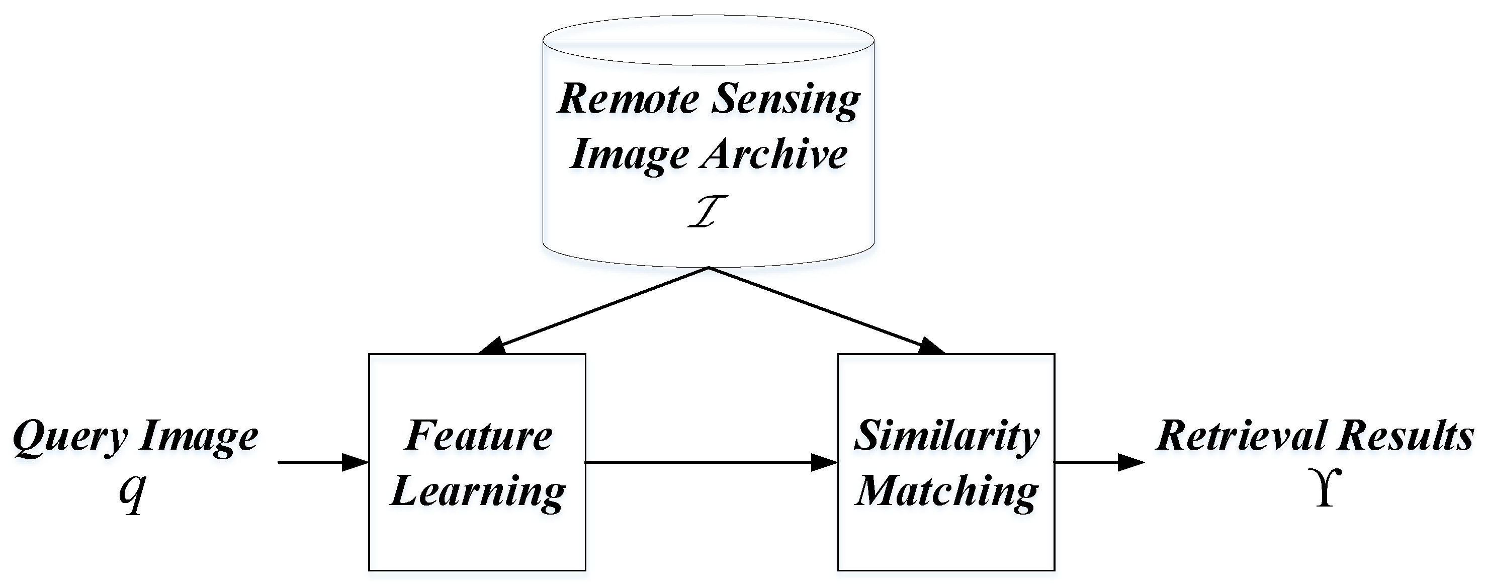
2.1. Remote Sensing Image Retrieval

RSIR is a popular research topic in the RS community, and there are many successful methods that were proposed in the last decades. Here, we divide them into two groups for review. In the first group, the proposed methods aim to develop effective content descriptors or similarity measures for RSIR. Datcu et al. [42] presented a knowledge-driven information mining method in 2003. In this method, the stochastic model (Gibbs Markov random field) was used to extract the RS images’ texture features from the content aspect. Meanwhile, the unsupervised clustering scheme was developed to reduce the feature vectors’ dimension. In addition, Bayesian networks were introduced to capture the users’ interests from the semantic level. Combining them together, satisfactory retrieval results could be acquired. Yang et al. [43] presented an RSIR method based on the bag-of-words (BOW) [44] features. Several key issues for constructing the BOW features are discussed in detail for RS images, such as scale invariant feature transform (SIFT) [45], codebook size, etc. Based on the BOW features, the retrieval results could be obtained using the common distance measures. With the help of CNN, Tang et al. [46] proposed an unsupervised deep feature learning method for RSIR. Both the complex contents and the multi-scale information of the RS images were taken into account in this method. Apart from the mentioned feature extraction/learning methods, there are still many algorithms that focus on similarity measures. A region-based distance was proposed for Synthetic Aperture Radar (SAR) image content retrieval [47]. In this method, SAR image was segmented into several regions using the texture, brightness and shape features first. Then, the distances between SAR images were formulated as the integration of the dissimilarities of multiple regions. Tang et al. [48] introduced a fuzzy similarity measure to complete the RSIR. Similar to the approach presented in [47], the SAR image was divided into different regions first. Then, the fuzzy theory was chosen to represent different regions, which could decrease the negative influence of segmentation uncertainty. Finally, the formulation of resemblance between SAR images was transformed into calculating the similarities between fuzzy sets. Li et al. [49] developed a collaborative affinity metric fusion method to measure the similarities between high-resolution RS images for RSIR. First, the contributions of handcrafted and deep features were combined under the graph theory. Then, the resemblance between RS images was defined as the affinity values between the nodes within the graph.

In the second group, the researchers concentrate their efforts on improving the initial retrieval results. Some of them use the supervised relevance feedback (RF) framework to enhance retrieval performance. Ferecatu and Boujemaa [50] proposed an active learning (AL) driven RF method to improve retrieval performance. To ease the users’ burden of sample selection, AL was introduced in the RF iteration. Meanwhile, the authors proposed the most ambiguous and orthogonal (MAO) principle under the support vector machine (SVM) paradigm to ensure the selected samples are useful. Finally, the initial retrieval results were reranked using the SVM classifier. Another AL driven RF method was introduced in [51]. Besides the uncertainty and diversity (which correspond to the MAO principle), the density of samples was also taken into account during the sample selection. To overcome the limitation of a single AL method, a multiple AL-based RF method was proposed in [48]. Diverse AL algorithms were embedded in the RF framework to generate different reranked results. Then, those results were fused in the relevance score level to obtain the final retrieval results. Apart from the RF methods, other researchers select the unsupervised reranking techniques to improve the initial retrieval results. Tang et al. [52] developed an image reranking approach for SAR images based on the multiple graphs fusion. First, diverse SAR-oriented visual features were extracted, and the relevant scores were estimated in multiple feature spaces. Then, a model-image matrix was constructed based on the estimated scores for calculating the similarities between SAR images. Finally, a fully connected graph was established using the obtained similarities to accomplish the image reranking. Another image reranking method was developed for RS images [53], in which the retrieval improvement was achieved in a coarse-to-fine manner.

2.2. Learning to Hash

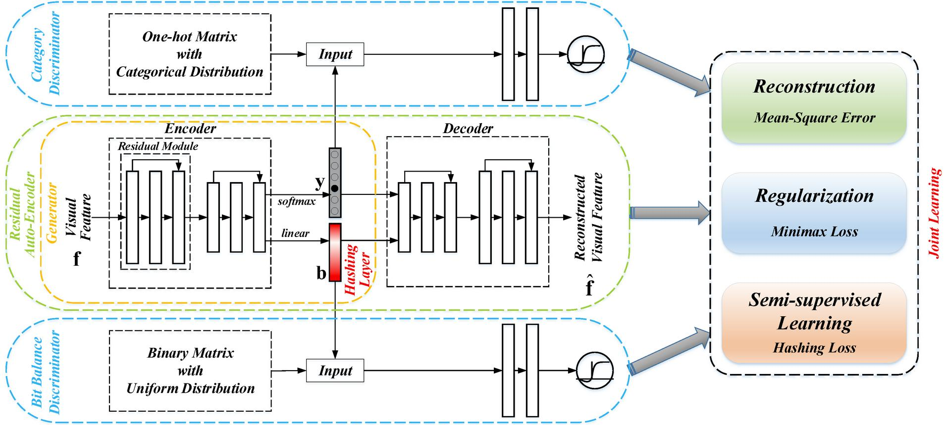
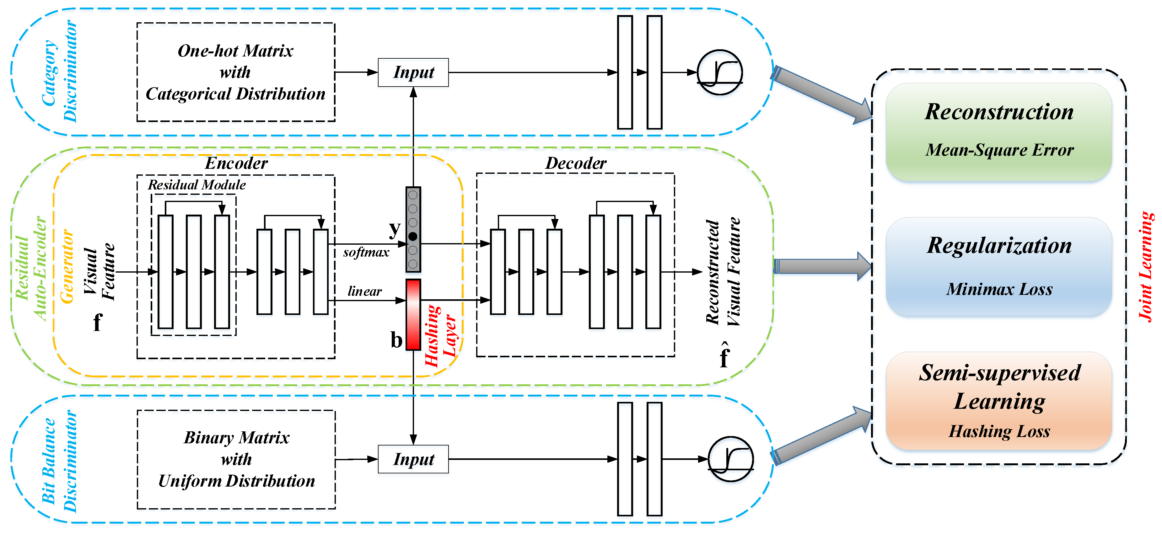
We roughly divide the existing learning to hash methods into two groups according to if the deep neural network is added in hash learning or not. The methods within the first group aim to develop effective hashing functions without the help of deep learning, and we name them non-deep hashing. Weiss et al. [26] proposed the spectral hashing to obtain the binary codes with the consideration of the semantic relationships between data-points. The authors transformed the hash learning into the graph partitioning and developed the spectral algorithm to complete the coding problem with the relaxation. Based on the spectral hashing, the kernelized version was proposed [54]. Through adding the kernel functions, the image contents represented by the original visual features could be fully mapped to the hash codes, which enhances the hashing performance. Heo et al. [55,56] proposed the spherical hashing to learn the hash functions for mapping more spatially coherent images into similar binary codes. In addition, the spherical hamming distance was developed to match up the spherical hashing. Shen et al. [57] developed the supervised discrete hashing to simplify the hash optimization (NP-hard problem in general) by reformulating the objective function using an auxiliary variable. Through dividing the NP-hard hashing into several sub-problems, the normal regularization algorithm (such as cyclic coordinate descent) could be used to optimize the binary codes. A two-step hash learning algorithm was introduced in [58]. The first step aimed to define a unified formulation for both supervised and unsupervised hashing. The second step focused on transforming the bit learning into the binary quadratic problem. In the RS community, Demir and Bruzzone [5] selected the kernel-based nonlinear hashing method [59] to complete the large-scale RSIR. The comprehensive experiments proved the feasibility of hash learning for RS images. Although the methods discussed above are reasonable and feasible, their performance is still limited due to the input data which is the handcrafted visual feature.

In the second group, the deep neural network is incorporated to accomplish hash learning, we name them deep hashing. The earliest deep hash learning method might be semantic hashing [60], in which the restricted Boltzmann machine (RBM) was introduced to map the documents from the original feature space to the binary space. The learning process was completed by two steps, i.e., pre-training and fine-tuning, which aim to generate the low-dimensional vectors and binary-like codes, respectively. Xia et al. [36] proposed another two-stage deep hashing method named supervised hashing. In the first stage, the approximate hash codes of the training images were obtained by decomposing the pairwise similarity matrix without considering the visual contents. Then, a CNN model was developed to learn the deep features and final hash codes with the guidance of semantic labels and obtained approximate hash codes. An end-to-end deep hashing approach was presented in [34] to deal with multi-label image retrieval. Both the semantic ranking and CNN model were combined to learn hash functions so that the obtained hash codes could remain the multiple similarities between the images in the semantic space. Do et al. [61] developed a binary deep neural network to learn the hash codes in an unsupervised manner. Considering the key points within the hash learning, the authors designed the specific loss function and utilized the alternating optimization algorithm with algebraic relaxation to solve it. Then, they expanded the proposed network to the supervised version to reach the stronger performance. To reduce the time cost of hash learning, Jiang and Li [62] introduced an asymmetric deep supervised hashing model. In this model, only the query images’ hash functions were learned via CNN. The target images’ hash codes were learned by the asymmetric pairwise loss function directly. From this point, the whole hash learning process could be speeded up obviously. In the RS community, Li et al. [40,63] proposed a set of deep hashing methods to deal with the single source and multi-source RSIR tasks. In [40], with the consideration of the characteristics of single source RS images, the authors developed the deep CNN model with the pairwise loss function to learn the hash codes. Two scenarios, i.e., the labeled images were limited or sufficient, were taken into account during the network training. In [63], the source-invariant deep hashing CNN was proposed to cope with the cross-source RSIR task. Besides the normal intra-source pairwise constraints, authors developed the specific loss term for inter-source. Then, the alternating learning strategy was proposed to train the network. The experimental results verified the effectiveness of the proposed method.

3. Methodology

The proposed SDAH network is discussed in this section. Before explaining our SDAH, the adversarial auto-encoder (AAE) is introduced first.

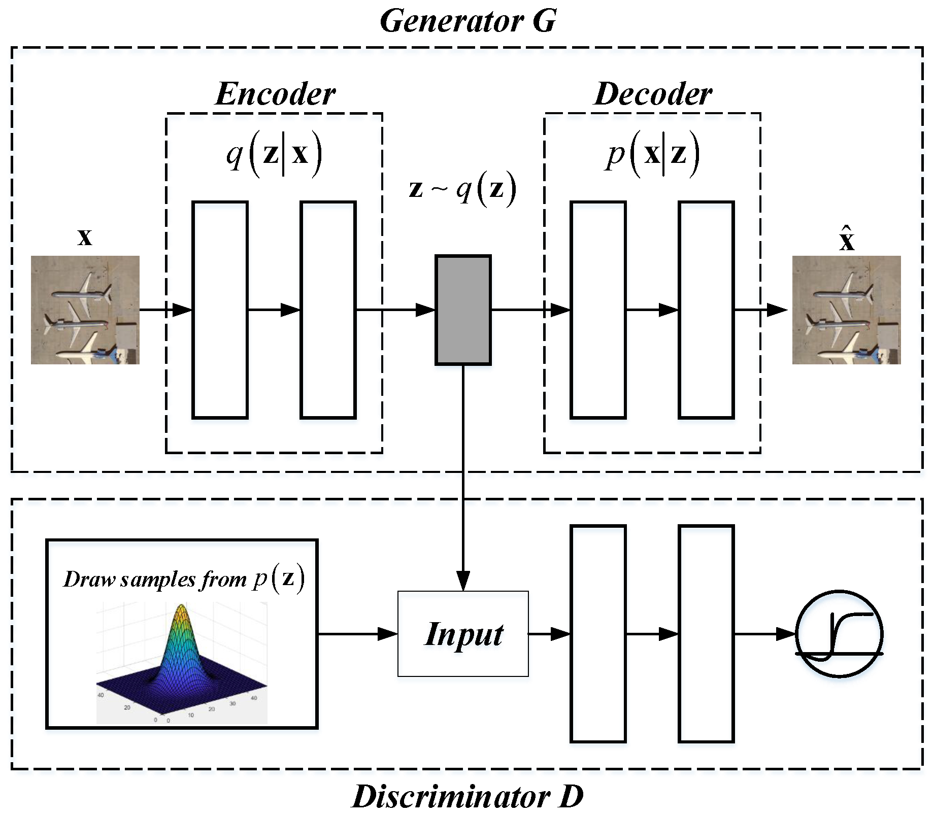
3.1. Adversarial Autoencoder

AAE model [41] is an expansion of auto-encoder (AE). Through the adversarial learning (which is proposed in GAN [64]), AAE can not only learn the latent feature but also impose a certain distribution on the learned feature. From this point, AAE can be regarded as the probabilistic AE. The basic framework of AAE is shown in Figure 2.

There are two networks within the AAE model, including the generator G and discriminator D. The generator G is actually an AE, which aims at learning the latent feature $\mathbf{z}$ from the input data $\mathbf{x}$ according to the reconstruction error. From the view of distribution, the encoding can be formulated as

$$q\left(\mathbf{z}\right)={\int }_{\mathbf{x}}q\left(\left.\mathbf{z}\right|\mathbf{x}\right)p_d\left(\mathbf{x}\right)d\mathbf{x},$$

(1)

where $q\left(\mathbf{z}\right)$ indicates the aggregated posterior distribution of the latent feature $\mathbf{z}$, $q\left(\left.\mathbf{z}\right|\mathbf{x}\right)$ means the encoding distribution, and $p_d\left(\mathbf{x}\right)$ denotes the data distribution. The decoder uses the latent feature $\mathbf{z}$ to generate the reconstructed data $\widehat{\mathbf{x}}$. The generator G can be trained by minimizing the error between $\mathbf{x}$ and $\widehat{\mathbf{x}}$, which is often measured by the mean square error (MSE). The discriminator D is a normal multi-layer network, which is added on the top of the learned feature $\mathbf{z}$ for guiding $q\left(\mathbf{z}\right)$ to match an arbitrary prior distribution $p\left(\mathbf{z}\right)$. The goal of D is distinguishing if the input vector follows the prior distribution $p\left(\mathbf{z}\right)$ or not. The AAE model can be trained in the minimax optimization manner which is proposed in [64]. The solution of the minimax optimization is formulated as

$$\underset{G}{min}\underset{D}{max}V\left(D,G\right)=E_{\mathbf{x}\tilde{}{p}_{data}\left(\mathbf{X}\right)}\left[logD\left(\mathbf{x}\right)\right]+E_{\mathbf{x}\tilde{}{p}_z\left(z\right)}\left[log\left(1-D\left(G\left(z\right)\right)\right)\right].$$

(2)

Apart from the basic model, there are still other two models in the AAE framework. One is supervised AAE, and the other is semi-supervised AAE. For supervised AAE, the label information is incorporated in the decoding stage. First, the label is converted into the one-hot vector. Then, both the label vector and the latent feature $\mathbf{z}$ are fed to the decoder of G to reconstruct the input data $\mathbf{x}$. For semi-supervised AAE, the label information is embedded through the adversarial learning. Suppose there are two prior distributions, i.e., categorical and expected distributions. For generator G, after the encoding, two vectors are generated, including the discrete class variable $\mathbf{y}$ and the continuous latent feature $\mathbf{z}$. Then, they are used to reconstruct the input data by the decoder. For discriminator $D_1$, the prior categorical distribution is imposed to regularize $\mathbf{y}$ for ensuring the discrete class variable do not carry any information of latent feature $\mathbf{z}$. For discriminator $D_2$, the expected distribution is imposed to force the the aggregated posterior distribution of latent feature $\mathbf{z}$ matches the predefined distribution. The reconstructed error, regularization loss and the semi-supervised classification error should be considered under the adversarial learning framework.

Due to the characteristic of the AAE model, especially the semi-supervised version, it can be used to learn the hash code inherently. First, the hash code can be adversarial leaned through imposing a prior uniform distribution with binary values. Second, under the semi-supervised learning framework, the semantic information (labels) of samples can be embedded, which can guarantee the learned binary features are discriminative. In addition, the volume of the labeled data is not large, which leads the hashing method feasible in practice.

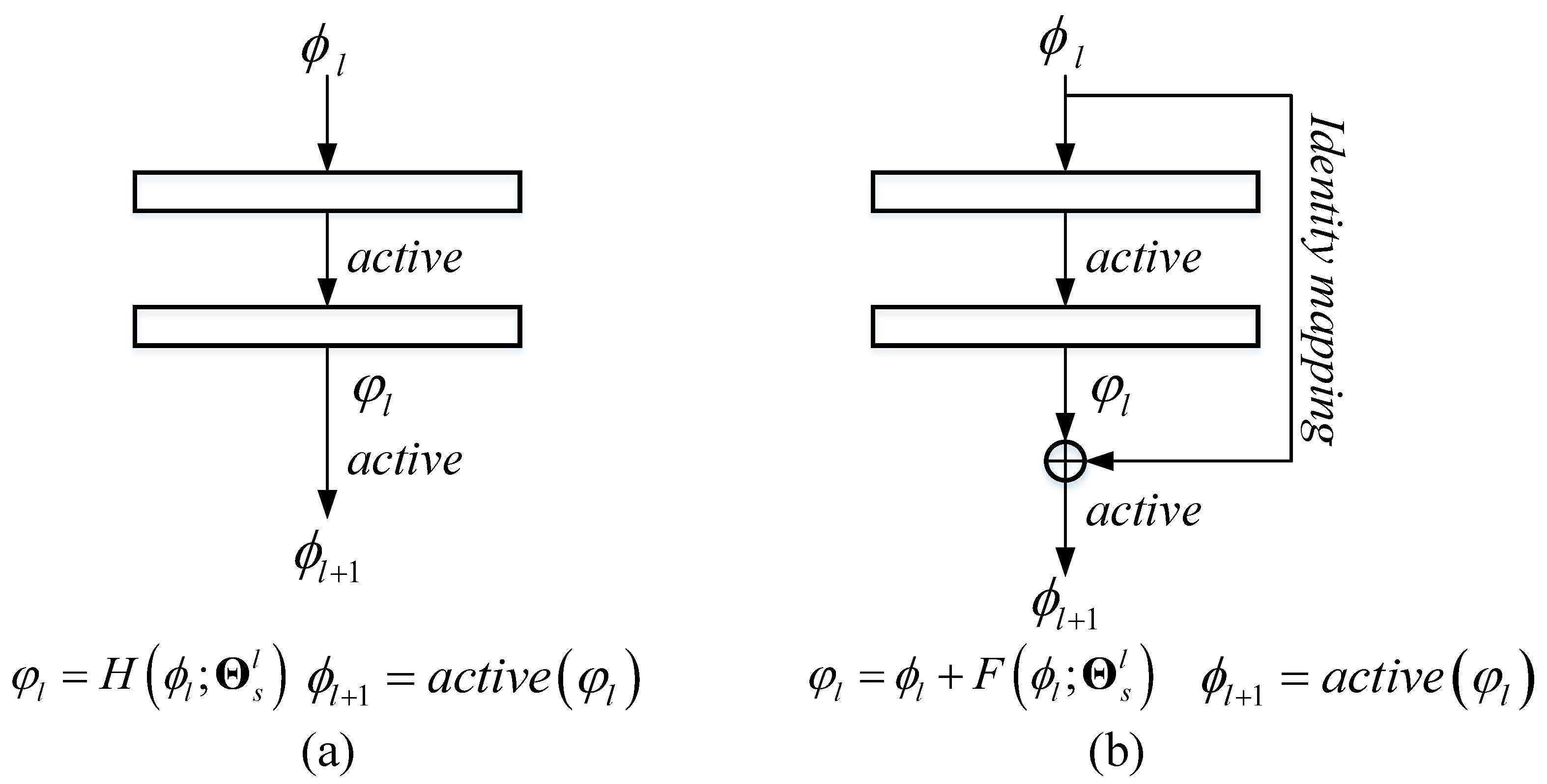
3.2. Proposed Deep Hashing Network

Based on the semi-supervised AAE model, we propose our SDAH in this section. Its framework is exhibited in Figure 3, which consists of three components, they are, residual auto-encoder (RAE) based generator G, category discriminator $D_c$, and uniform discriminator $D_u$. Now, we introduce them in detail.

To illustrate the generator G clearly, we first introduce RAE network. Similar to the AE model, there are three components in our RAE, including encoder, hidden layer and decoder. Nevertheless, the following modification is carried out for developing RAE. First, to reduce the difficulty of training and enrich the information of the latent features (i.e., the outputs of the encoder), the residual module [65] is introduced into our RAE. Through adding the residual module, not only the problems of gradient vanishing and degradation can be mitigated but also the layer-wise information loss would be decreased. Second, we divide the hidden layer into two parts, including the class variable $\mathbf{y}$ and the hash code $\mathbf{b}$. The class variable $\mathbf{y}$ is used to accomplish the semi-supervised learning, while the hash code $\mathbf{b}$ is our final target. The work flow of RAE can be summarized as follows. When users input the visual feature $\mathbf{v}$, the encoder with the residual module maps it into $\mathbf{y}$ and $\mathbf{b}$. Then, both $\mathbf{y}$ and $\mathbf{b}$ are fed into the residual decoder for the reconstructed data $\widehat{\mathbf{v}}$. The generator G of our SDAH model is the encoder of RAE, which focuses on generating the class and hash variables.

Generally speaking, the class information is always described by the one-hot vector (single class scenario). However, the generated class variable $\mathbf{y}$ in our SDAH is continuous. Thus, the category discriminator $D_c$ is developed to impose the categorical distribution [66] on $\mathbf{y}$. Note that the categorical distribution is a discrete probability distribution, which describes the results of a random variable that belongs one of c categories. The category discriminator $D_c$ is a normal multi-layer neural network with the softmax output. Its main function is distinguishing if a sample generated by G or not. To this end, we construct a one-hot matrix with the categorical distribution as the “true” input of $D_c$. Apart from regularizing $\mathbf{y}$ to follow the categorical distribution, $D_c$ can also ensure the generated $\mathbf{y}$ only contains the class information. Thus, these generated label representations can be used to accomplish the semi-supervised learning directly.

Besides $D_c$, another multi-layer network is also developed to regularize the generated latent hash code $\mathbf{b}$. Here, we record it uniform discriminator $D_u$. Due to the characteristic of the back propagation algorithm, the generated $\mathbf{b}$ is actually a continuous variable rather than a discrete binary code with value 0/1. To obtain the expected binary code, we impose the binary uniform distribution on $\mathbf{b}$ using $D_u$. First, a binary matrix with uniform distribution is constructed to be the “true” data for $D_u$. Second, $D_u$ forces the generated $\mathbf{b}$ to follow the prior binary uniform distribution by the adversarial learning. Through adding the uniform discriminator $D_u$, we can not only learn the pseudo-binary codes but also ensure the codes keep bit balanced. Here, the pseudo-binary code means the values of each bit in $\mathbf{b}$ are concentrated around 0 and 1.

3.3. Learning Strategy of Proposed Hashing Network

After introducing the components of our SDAH model, the learning strategy is discussed in this section. The network training can be divided into three parts, including unsupervised reconstruction, adversarial regularization and semi-supervised learning. Before describing them in detail, we first define some important notations for clarity. Suppose there is an image dataset $\mathcal{I}=\left\{I_1,\cdots I_N\right\}$ with N RS images. The visual features $\mathbf{V}=\left\{{\mathbf{v}}_1,\cdots ,{\mathbf{v}}_N\right\}$ of those images have been obtained. The semantic labels $\left\{{\mathbf{s}}_1,\cdots ,{\mathbf{s}}_n\right\}$ of a small number of RS images are provided, where $n\ll N$.

3.3.1. Unsupervised Reconstruction

The main target of unsupervised reconstruction is to train the generator G using all of N samples, and this step is accomplished by the RAE model.

Similar to the traditional AE model, we assume that the encoder of RAE is represented by $f\left(·\right)$, while the decoder of RAE is denoted by $g\left(·\right)$. Thus, for an input sample $\mathbf{v}$, the RAE model can be defined as

$$\left[\mathbf{y},\mathbf{b}\right]=f\left(\mathbf{v};{\mathbf{\Theta }}_r\right),\widehat{\mathbf{v}}=g\left(\mathbf{y},\mathbf{b};{\mathbf{\Theta }}_r\right),$$

(3)

where $\widehat{\mathbf{v}}$ means the reconstructed sample, and ${\mathbf{\Theta }}_r$ indicates the weights of RAE. To estimate the encoding and decoding functions, we minimize the mean squared error between $\mathbf{v}$ and $\widehat{\mathbf{v}}$. The optimization can be formulated as

$${\mathcal{L}}_{RAE}=\underset{{\Theta }_r}{argmin}\sum _{i=1}^N{∥{\mathbf{v}}_i-{\widehat{\mathbf{v}}}_i∥}_2^2=\underset{{\Theta }_r}{argmin}\sum _{i=1}^N{∥{\mathbf{v}}_i-g\left(f\left(\mathbf{v};{\mathbf{\Theta }}_r\right);{\mathbf{\Theta }}_r\right)∥}_2^2,$$

(4)

Different from the conventional AE model, the basic unit of RAE is the residual block rather than the normal fully connection block. Suppose the input of the lth residual block is ${\varphi }_l$, and the weights corresponding to the lth residual block is ${\mathbf{\Theta }}_r^l=\left\{{\mathbf{\Theta }}_r^{l,i},1\le i\le n_l\right\}$, where $n_l$ denotes the number of layers in the residual block. Therefore, the output of the lth residual block is

$${\phi }_l={\varphi }_l+F\left({\varphi }_l;{\mathbf{\Theta }}_r^l\right),$$

(5)

where $F\left(·\right)$ means the residual function that completed by several fully connection layers. After the element-wise addition, the input of the $(l+1)$th residual block can be defined as ${\varphi }_{l+1}=active\left({\phi }_l\right)$, where $active\left(·\right)$ denotes the activation function. If we select the linear activation function, the input of the $(l+1)$th residual block can be written as

$${\varphi }_{l+1}={\varphi }_l+F\left({\varphi }_l;{\mathbf{\Theta }}_r^l\right).$$

(6)

Consequently, the recurrence formula of the L residual blocks can be defined as

$${\varphi }_L={\varphi }_l+\sum _{i=l}^{L-1}F\left({\varphi }_i;{\mathbf{\Theta }}_r^i\right).$$

(7)

When we use the backward propagation algorithm to optimize ${\mathcal{L}}_{RAE}$, the chain rule of derivative should be adopted, i.e.,

$$\frac{\partial {\mathcal{L}}_{RAE}}{\partial {\varphi }_l}=\frac{\partial {\mathcal{L}}_{RAE}}{\partial {\varphi }_L}\frac{\partial {\varphi }_L}{\partial {\varphi }_l}=\frac{\partial {\mathcal{L}}_{RAE}}{\partial {\varphi }_L}\left(1+\frac{\partial }{\partial {\varphi }_l}\sum _{i=l}^{L-1}F\left({\varphi }_i;{\mathbf{\Theta }}_r^i\right)\right).$$

(8)

To further explain the residual block, we exhibit a comparison between the fully connection block and the residual block in Figure 4. Figure 4a shows a normal fully connection block. The output of the $\left(l\right)$th block ${\phi }_l$ can be obtained using mapping function $F\left(·\right)$ directly. In contrast, the output of the $\left(l\right)$th residual block (displayed in Figure 4b) should be acquired by the summation of ${\varphi }_l$ and results of $F\left(·\right)$.

After training the RAE, we can obtain the generator G of our SDAH model, which is actually the encoder of RAE.

3.3.2. Adversarial Regularization

When we learn the generator G, two latent variables $\mathbf{y}$ and $\mathbf{b}$ can also be obtained. As mentioned in Section 3.2, we wish that $\mathbf{y}$ could reflect the semantic label information and $\mathbf{b}$ could be the expected binary code. To this end, two discriminators $D_c$ and $D_u$ are developed to impose the certain distributions on $\mathbf{y}$ and $\mathbf{b}$.

Now, the problem is how to construct the “true” input data with the proper distribution for two discriminators. For $D_c$, we construct the “true” input data as follows. First, $n_{ca}$ one-hot column vectors ${\mathbf{m}}_{ca}\in {\mathbb{R}}^{c\times 1}$ are generated randomly, where c means the number of semantic class. Then, we combine them together to construct a matrix ${\mathbf{M}}_{ca}\in {\mathbb{R}}^{c\times n_{ca}}$. It is not difficult to find that the constructed ${\mathbf{M}}_{ca}$ follows the category distribution naturally. For $D_u$, we construct the “true” input data under the following conditions. First, we define a matrix ${\mathbf{M}}_{un}\in {\mathbb{R}}^{K\times n_{un}}$ with the uniform distribution, where K indicates the length of expected hash code. In addition, the elements within ${\mathbf{M}}_{un}$ are 0 or 1. Then, we further let ${\mathbf{M}}_{un}·{\mathbf{M}}_{un}^T=\mathbf{I}·\left(K/2\right)$.

When the “true” input data for discriminators is decided, the next step is imposing the prior distributions on the generated latent variables through the adversarial learning. For clarity, we separate the generator G into $G_c$ and $G_u$, which correspond to $\mathbf{y}$ and $\mathbf{b}$, respectively. Then, the adversarial regularization procedure can be formulated by Equations (9) and (10).

$$\underset{G_c}{min}\underset{D_c}{max}{E}_{\mathbf{x}\sim p\left({\mathbf{M}}_{ca}\right)}\left[log{D}_c\left(\mathbf{x}\right)\right]+E_{\mathbf{y}\sim p\left(\mathbf{y}\right)}\left[log\left(1-D_c\left(G_c\left(\mathbf{y}\right)\right)\right)\right]$$

(9)

$$\underset{G_u}{min}\underset{D_u}{max}{E}_{\mathbf{x}\sim p\left({\mathbf{M}}_{un}\right)}\left[log{D}_u\left(\mathbf{x}\right)\right]+E_{\mathbf{b}\sim p\left(\mathbf{b}\right)}\left[log\left(1-D_u\left(G_u\left(\mathbf{b}\right)\right)\right)\right]$$

(10)

There is another point we want to explain further: the value of $n_{ca}$ and $n_{un}$. The data used for training the deep neural network are usually divided into several batches. For different batches, we would construct different “true” data with the same distribution for $D_c$ and $D_u$. Thus, the values of $n_{ca}$ and $n_{un}$ are equal to the batch size $n_b$.

3.3.3. Semi-Supervised Learning

After the unsupervised reconstruction and the adversarial regularization, we can obtain the latent variable $\mathbf{y}$ with the category distribution and the binary-like variable $\mathbf{b}$ with the uniform distribution. Nevertheless, since there are no other specific operations, the current code $\mathbf{b}$ does not have any discriminative information, which is not proper for the retrieval task. Thus, we develop the semi-supervised learning part to improve $\mathbf{b}$.

First, to ensure $\mathbf{b}$ is discriminative, we adopt the classification loss function to embed the semantic information. As mentioned at the beginning of this section, there are n samples with the semantic labels $\left\{{\mathbf{s}}_1,\cdots ,{\mathbf{s}}_n\right\}$. Assume that the class variables $\left\{{\mathbf{y}}_1,\cdots ,{\mathbf{y}}_n\right\}$ corresponding to those samples have been obtained. Then, the cross entropy function is selected to measure the classification error, and the formula is

$${\mathcal{L}}_{cls}=-\sum _i^n\left({\mathbf{s}}_{i}log{\mathbf{y}}_i\right).$$

(11)

Note that there are two common formats of the cross entropy function [66,67,68], and we select the current version (Equation (11)) since the softmax function is selected to accomplish the classification.

Second, to remain the similarity relationships between samples from the original feature space to hash code space, and further introduce the semantic label information, we design the similarity preserving loss function as follow,

$${\mathcal{L}}_{sim}=\sum _{i=1}^n\sum _{j=1}^n\left(r_{ij}{∥{\mathbf{b}}_i-{\mathbf{b}}_j∥}_2^2+\left(1-r_{ij}\right)max\left(m-{∥{\mathbf{b}}_i-{\mathbf{b}}_j∥}_2^2,0\right)\right),$$

(12)

where $r_{ij}$ indicates the semantic relationships between two samples, ${∥{\mathbf{b}}_i-{\mathbf{b}}_j∥}_2^2$ measures the distance between two samples, and $m>0$ denotes the margin parameter. For $r_{ij}$, when two samples belong to the same semantic class $r_{ij}=1$ and otherwise $r_{ij}=0$. This function constrains the similar samples should be mapped into similar hash codes.

To solve the proposed similarity preserving loss function using the back propagation algorithm, some characteristics of ${\mathcal{L}}_{sim}$ should be analyzed, including the convexity and the differentiability. For convexity, there are two terms within the objective function ${\mathcal{L}}_{sim}$, and both of them are the convex functions. In addition, since the value of $r_{ij}$ is equal to 0 or 1, the coefficient $\left(1-r_{ij}\right)$ is nonnegative. Thus, the linear combination of two terms, i.e., ${\mathcal{L}}_{sim}$, is also a convex function. For differentiability, due to the max operation, the object function is non-differentiable at some certain points [35]. To optimize Equation (12) smoothly, the sub-gradients is selected to replace the normal gradients. In addition, we define the sub-gradients to be $\mathbf{1}$ at such differentiable points. In detail, the two terms within ${\mathcal{L}}_{sim}$ are recorded ${\mathcal{L}}_{sim}^1$ and ${\mathcal{L}}_{sim}^2$ for short. Then, their sub-gradients can be formulated by Equations (13) and (14). After calculating the sub-gradients over the batches, the back propagation algorithm can be carried out normally.

$$\frac{\partial {\mathcal{L}}_{sim}^1}{\partial {\mathbf{b}}_i}=2r_{ij}\left({\mathbf{b}}_i-{\mathbf{b}}_j\right),\frac{\partial {\mathcal{L}}_{sim}^2}{\partial {\mathbf{b}}_j}=-2r_{ij}\left({\mathbf{b}}_i-{\mathbf{b}}_j\right).$$

(13)

$$\begin{array}{c}\frac{\partial {\mathcal{L}}_{sim}^2}{\partial {\mathbf{b}}_i}=\left\{\begin{array}{ccc}-2\left(1-r_{ij}\right)\left({\mathbf{b}}_i-{\mathbf{b}}_j\right)& ,& {∥{\mathbf{b}}_i-{\mathbf{b}}_j∥}_2^2<m\\ 0& ,& otherwise\end{array}\right.,\\ \frac{\partial {\mathcal{L}}_{sim}^2}{\partial {\mathbf{b}}_j}=\left\{\begin{array}{ccc}2\left(1-r_{ij}\right)\left({\mathbf{b}}_i-{\mathbf{b}}_j\right)& ,& {∥{\mathbf{b}}_i-{\mathbf{b}}_j∥}_2^2<m\\ 0& ,& otherwise\end{array}\right..\end{array}$$

(14)

Third, to decrease the quantization error, we introduce the following loss function in bit level [69],

$${\mathcal{L}}_{quan}=-\sum _{i=1}^n\sum _{k=1}^K{b}_i^{k}log\left(b_i^k\right)+\left(1-b_i^k\right)log\left(1-b_i^k\right),$$

(15)

where $b_i^k$ indicates the kth bit in the hash code. Through minimizing this function, the hash bits can be pushed toward 0 or 1. This can help to reduce the loss of quantization.

Finally, the discussed loss function is linearly combined together and the semi-supervised learning can be formulated as

$${\mathcal{L}}_{hash}=\underset{\mathbf{y},\mathbf{b}}{argmin}\left({\lambda }_c{\mathcal{L}}_{cls}+{\lambda }_s{\mathcal{L}}_{sim}+{\lambda }_q{\mathcal{L}}_{quan}\right),$$

(16)

where ${\lambda }_c$, ${\lambda }_s$ and ${\lambda }_q$ are the free parameters for adjusting the contribution of each term.

3.3.4. Flow of Learning Strategy

We adopt the stochastic learning method to train our SDAH model. The three parts discussed above are trained alternatively. In particular, the unsupervised reconstruction loss function ${\mathcal{L}}_{RAE}$ is optimized first to initial the parameters of the generator G. Then, the parameters of the generator G and discriminators $D_c$ and $D_u$ are updated by Equations (9) and (10). Third, the generated latent variables $\mathbf{y}$ and $\mathbf{b}$ are optimized using ${\mathcal{L}}_{hash}$. The first two steps are accomplished using all N samples, while the third step is achieved using n labeled samples. It is note that the learned variable $\mathbf{b}$ is a binary-like vector that the elements within the vector are near 1 or 0. To obtain the real discrete binary code, we set a threshold t. When $b_i>t$, $b_i=1$, and otherwise $b_i=0$. In this paper, we set $t=0.5$ unless otherwise stated.

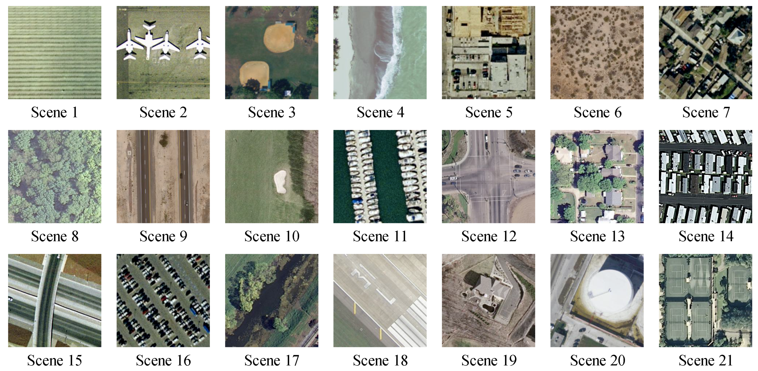
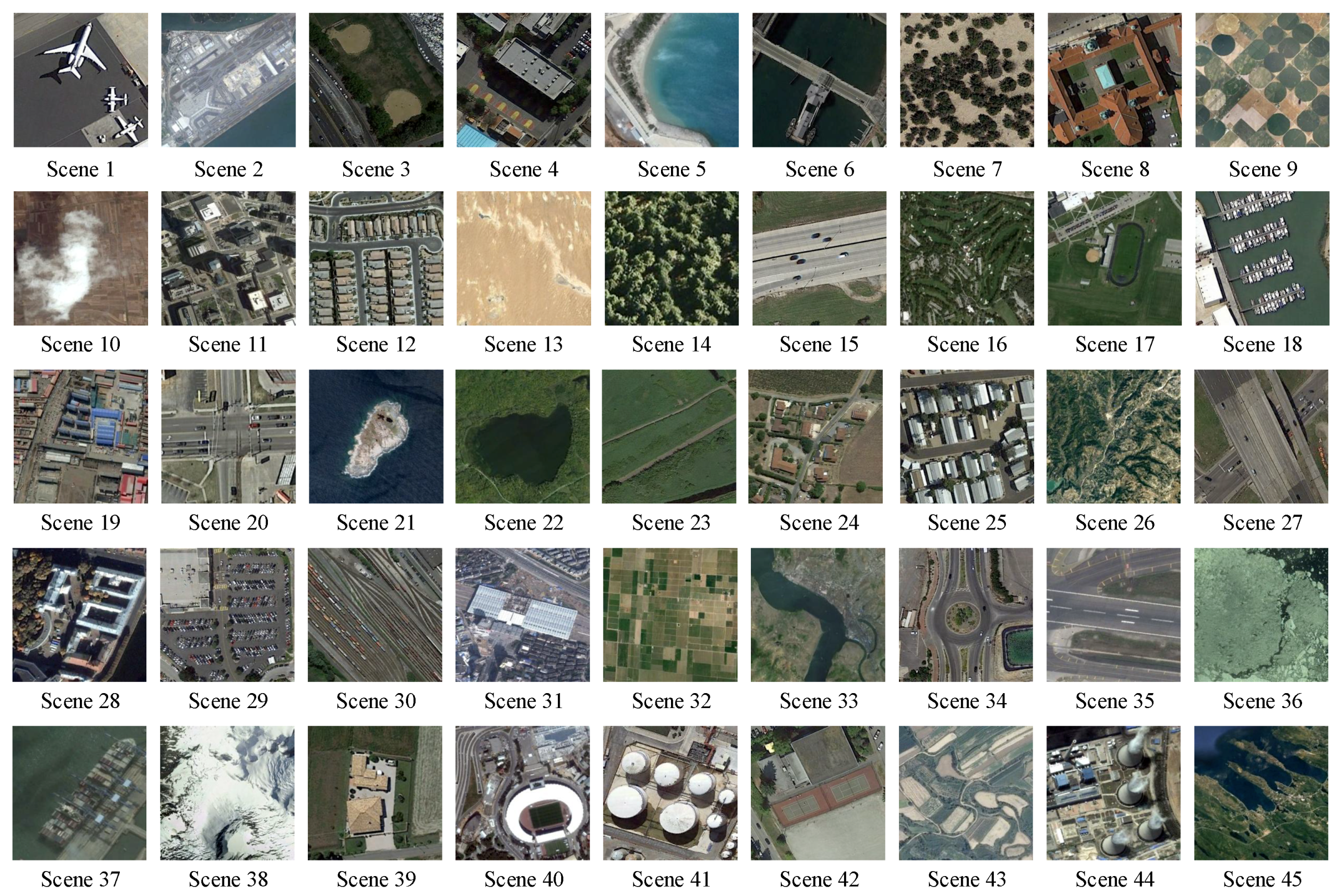
4. Dataset Introduction

To testify our SDAH model is effective for RSIR task, we selected three published RS image sets. The first one is a high resolution land-use image set constructed by University of California Merced [43,70]. We refer to it as UCM in this paper. There are 2100 RS images with the pixel resolution of one foot in UCM. Their size is $256\times 256$. All of those images are equally divided into 21 semantic categories, including “agricultural”, “airplane”, etc. The examples of RS images corresponding to each category are exhibited in Figure 5, and the names and volume of different scenes are summarized in

Table 1. Names and volume of different scenes in UCM dataset.

Scene Number	Scene	Volume	Scene Number	Scene	Volume
1	Agricultural	100	12	Intersection	100
2	Airplane	100	13	Medium Residential	100
3	Baseball Diamond	100	14	Mobile Home Park	100
4	Beach	100	15	Overpass	100
5	Buildings	100	16	Parking Lot	100
6	Chaparral	100	17	River	100
7	Dense Residential	100	18	Runway	100
8	Forest	100	19	Sparse Residential	100
9	Freeway	100	20	Storage Tanks	100
10	Golf Course	100	21	Tennis Court	100
11	Harbor	100

. The second one is an aerial image dataset constructed by Wuhan University and HuaZhong University of Science and Technology [71]. Here, we name it AID for short. In AID, there are 10,000 aerial images with the fixed size of $600\times 600$, and their pixel resolution covers from 0.5 m to 8 m. All of the images are partitioned into 30 semantic scenes, including “Airport”, “Bare Land”, etc. The number of images within each scene is not balanced. The scene with the minimal images (220) is “Baseball Field”, while the categories with maximum images (420) are “Pond” and “Viaduct”. Some examples of different scenes are exhibited in Figure 6, and their names and volume are displayed in

Table 2. Names and volume of different scenes in AID dataset.

Scene Number	Scene	Volume	Scene Number	Scene	Volume
1	Airport	360	16	Mountain	340
2	Bare Land	310	17	Park	350
3	Baseball Field	220	18	Parking	390
4	Beach	400	19	Playground	370
5	Bridge	360	20	Pond	420
6	Center	260	21	Port	380
7	Church	240	22	Railway Station	260
8	Commercial	350	23	Resort	290
9	Dense Residential	410	24	River	410
10	Desert	300	25	School	300
11	Farmland	370	26	Sparse residential	300
12	Forest	250	27	Square	330
13	Industrial	390	28	Stadium	290
14	Meadow	280	29	Storage tanks	360
15	Medium Residential	290	30	Viaduct	420

. The last one is a 45-scene-class RS image dataset published by Northwestern Polytechnical University [72], and we name it NWPU for short in this paper. There are 700 images for each scene category, and the spatial resolution of those images ranges from 0.2 m to 30 m. The size of images within NWPU is $256\times 256$. Some examples of different classes are displayed in Figure 7, and the names and volume of these scenes can be found in

Table 3. Names and volume of different scenes in NWPU dataset.

Scene Number	Scene	Volume	Scene Number	Scene	Volume
1	Airplane	700	24	Medium Residential	700
2	Airport	700	25	Mobile Home Park	700
3	Baseball Diamond	700	26	Mountain	700
4	Basketball Court	700	27	Overpass	700
5	Beach	700	28	Palace	700
6	Bridge	700	29	Parking Lot	700
7	Chaparral	700	30	Railway	700
8	Church	700	31	Railway Station	700
9	Circular Farmland	700	32	Rectangular Farmland	700
10	Cloud	700	33	River	700
11	Commercial Area	700	34	Roundabout	700
12	Dense Residential	700	35	Runway	700
13	Desert	700	36	Sea Ice	700
14	Forest	700	37	Ship	700
15	Freeway	700	38	Snow Berg	700
16	Golf Course	700	39	Sparse Residential	700
17	Ground Track Field	700	40	Stadium	700
18	Harbor	700	41	Storage Tank	700
19	Industrial Area	700	42	Tennis Court	700
20	Intersection	700	43	Terrace	700
21	Island	700	44	Thermal Power Station	700
22	Lake	700	45	Wetland	700
23	Meadow	700

.

5. Experiments

5.1. Experimental Settings

To generate the hash code using our SDAH, some preparatory work should be completed in advance. First, the structure of SDAH should be decided. Suppose the dimension of input data is d, the number of semantic classes is c, and the bit of expected hash codes is K. Then, our hashing network structure is summarized in

Table 4. Structure of our semi-supervised deep adversarial hashing.

Residual Auto-Encoder	Encoder (Generator)	$\mathit{d}\to \left({}^{\mathit{d}}/{}_2\to {}^{\mathit{d}}/{}_2\to {}^{\mathit{d}}/{}_2\right)\to \left({}^{\mathit{d}}/{}_4\to {}^{\mathit{d}}/{}_4\to {}^{\mathit{d}}/{}_4\right)$
	Latent	c, K
	Decoder	$\left({}^d/{}_4\to {}^d/{}_4\to {}^d/{}_4\right)\to \left({}^d/{}_2\to {}^d/{}_2\to {}^d/{}_2\right)\to d$
Category Discriminator		$c\to {}^d/{}_2\to {}^d/{}_4$
Uniform Discriminator		$K\to {}^d/{}_2\to {}^d/{}_4$

. Second, the training data for SDAH need to be prepared. We randomly selected 20% of images from the original dataset to be the training data. The influence of training data with different proportions is discussed in Section 5.4. Third, the visual features of the RS images need to be extracted. Here, to prove the effectiveness of SDAH, we adopted five common visual features. The details of the performance based on these visual features are discussed in Section 5.2. Fourth, the values of some parameters need to be decided, including the margin parameter m (Equation (12)), and the weighting parameters ${\lambda }_c$, ${\lambda }_s$ and ${\lambda }_q$ (Equation (16)). All of the parameters were tuned by the k-fold cross-validation in this study. For various RS image archives and diverse visual features, the optimal parameters are different. The details are displayed in Section 5.2. In addition, we used the Adam algorithm [73] to optimize our adversarial hashing network. The learning rate and iteration were set to $1\times {10}^{-4}$ and 50, respectively. All experiments were accomplished using an HP 840 high-performance computer with GeForce GTX Titan X GPU.

We selected precision–recall (P-R curve) and mean average precision (MAP) to verify SDAH’s retrieval behavior numerically. Assume that we obtain $n_r$ retrieval results for a query image $\mathbf{q}$. The number of correct retrieval results is $n_{rc}$, and the number of the correct target images within the archive is $n_{rt}$. Thus, the precision and recall can formulated as ${}^{n_{rc}}/{}_{n_r}$ and ${}^{n_{rc}}/{}_{n_{rt}}$. Here, we define that a retrieved/target image is correct if it belongs to the same semantic category as query. Furthermore, let us impose the labels $\left\{l_1,l_2,\cdots ,l_{n_r}\right\}$ on the results. If the retrieved image is correct, $l_i=1$, and otherwise $l_i=0$. Then, MAP can be defined as

$$\frac{1}{Q}\sum _Q\left(\frac{1}{n_r}\sum _{i=1}^{n_r}\frac{l_i}{i}\sum _{j=1}^i{l}_i\right),$$

(17)

where Q means the number of query images.

5.2. Retrieval Performance Based on Different Visual Features

The performance of our SDAH model based on different visual features was studied. Considering the characteristics of RS images, we selected five visual features to represent RS images:, SIFT-based BOW features [70], the outputs of the seventh fully connected layer of Alexnet [31] and VGG16 [74], and the outputs of the seventh fully connected layer of fine-tuned Alexnet and VGG16. These features are common in the RS community [43,75,76]. Here, we refer to them as BOW, AlexFC7, VGG16FC7, AlexFineFC7, and VGG16FineFC7, respectively, for short. Among those features, BOW is mid-level and theothers are high-level features. To be fair, their dimension was set to 4096. In addition, 80% of images from RS archives were selected randomly to fine tune two deep networks for feature extraction. As mentioned above, the parameters (m, ${\lambda }_c$, ${\lambda }_s$, and ${\lambda }_q$) of our model depend on the different input visual features. After the k-fold cross-validation, the optimal parameters for different features and different RS image archives are displayed in

Table 5. Optimal parameters for different visual features and different image archives.

		BOW	AlexFC7	VGG16FC7	AlexFineFC7	VGG16FineFC7
UCM	${\lambda }_c$	0.50	0.20	0.90	0.60	0.40
	${\lambda }_s$	0.50	0.75	0.70	0.95	0.80
	${\lambda }_q$	0.65	0.05	0.05	0.20	0.10
	m	2.60	1.40	1.00	2.60	4.00
AID	${\lambda }_c$	1.00	0.45	0.50	0.30	0.35
	${\lambda }_s$	0.85	0.95	0.85	0.80	0.70
	${\lambda }_q$	0.01	0.01	0.01	0.01	0.01
	m	1.60	2.40	1.40	2.40	2.20
NWPU	${\lambda }_c$	0.90	0.95	0.80	0.25	0.90
	${\lambda }_s$	0.10	0.55	0.45	0.60	0.10
	${\lambda }_q$	0.05	0.01	0.01	0.01	0.05
	m	3.00	3.00	2.00	3.00	3.00

.

The experimental results are exhibited in

Table 6. Retrieval mean average precision counted on three archives based on different visual features using Top 50 retrieval results.

			BOW	AlexFC7	VGG16FC7	AlexFineFC7	VGG16FineFC7
UCM	Baseline		0.3338	0.4815	0.4613	0.6551	0.8027
	Hash codes bits	32	0.4362	0.7064	0.6414	0.8164	0.8994
		64	0.4429	0.7314	0.7001	0.8214	0.9173
		128	0.4503	0.7319	0.7316	0.8286	0.9225
		256	0.4734	0.7471	0.7369	0.8319	0.9277
		512	0.4801	0.7572	0.7503	0.8428	0.9269
AID	Baseline		0.2783	0.4683	0.4240	0.8276	0.9516
	Hash codes bits	32	0.3850	0.5975	0.6234	0.9230	0.9623
		64	0.4943	0.7228	0.6625	0.9379	0.9673
		128	0.5018	0.7346	0.7064	0.9394	0.9754
		256	0.5114	0.7519	0.7284	0.9448	0.9755
		512	0.5159	0.7641	0.7319	0.9466	0.9779
NWPU	Baseline		0.2284	0.4128	0.4123	0.6981	0.9044
	Hash codes bits	32	0.3469	0.6020	0.6181	0.8715	0.9324
		64	0.3609	0.6557	0.6234	0.8816	0.9572
		128	0.4048	0.6717	0.6523	0.8856	0.9614
		256	0.4524	0.6727	0.6708	0.8916	0.9688
		512	0.4676	0.6823	0.6795	0.8988	0.9710

, which are from three datasets using the Top 50 retrieval results. The “Baseline” in the table indicates the retrieval performance of visual features. For measuring the similarities between visual feature vectors, we selected Cosine (BOW) and L2-norm (AlexFC7, VGG16FC7, AlexFineFC7, and VGG16FineFC7) distances. The retrieval results were obtained according to the distance orders. For our hash codes, we set their length to be 32, 64, 128, 256, and 512, respectively, to study their retrieval behavior. Moreover, we selected the hamming distance to weigh the resemblance between hash codes. The retrieval results were also obtained in accordance with the distance orders.

In Table 6, we can easily find the following points. First, our SDAH model can generate useful hash codes based on different visual features. The strongest hash codes were obtained from the VGG16FineFC7 features, while the weakest binary vectors were learned using BOW features. This illustrates that the original visual features are important to hash learning. In other words, we could obtain the satisfactory hash codes if the original visual features can represent the complex contents within RS images well. The current visual features, from the mid-level to the high-level, capture the RS images’ contents from different aspects. Nevertheless, it is obvious that the fine-tuned VGG16 explores more useful information from images, which can be proved by the “Baseline” scores. Thus, the hash codes based on VGG16FineFC7 features achieve the best retrieval performance. Second, the retrieval performance of hash codes is better than that of the original visual features. The reason is that we introduce the semantic information into our hashing network, which can enhance the discrimination of the hash codes. Third, the hash codes’ retrieval behavior becomes stronger with the increase of the bit, which demonstrates that longer codes perform better. This is owing to our adversarial learning framework and the specific hashing function, which ensures the obtained binary codes are bit-balanced and low quantization loss. Thus, the longer codes bring richer information so that better performance can be reached. The encouraging experimental results displayed in Table 6 prove that our SDAH is useful to hash learning. For clarity, we fix AlexFineFC7 to be the input data for the rest of the experiments.

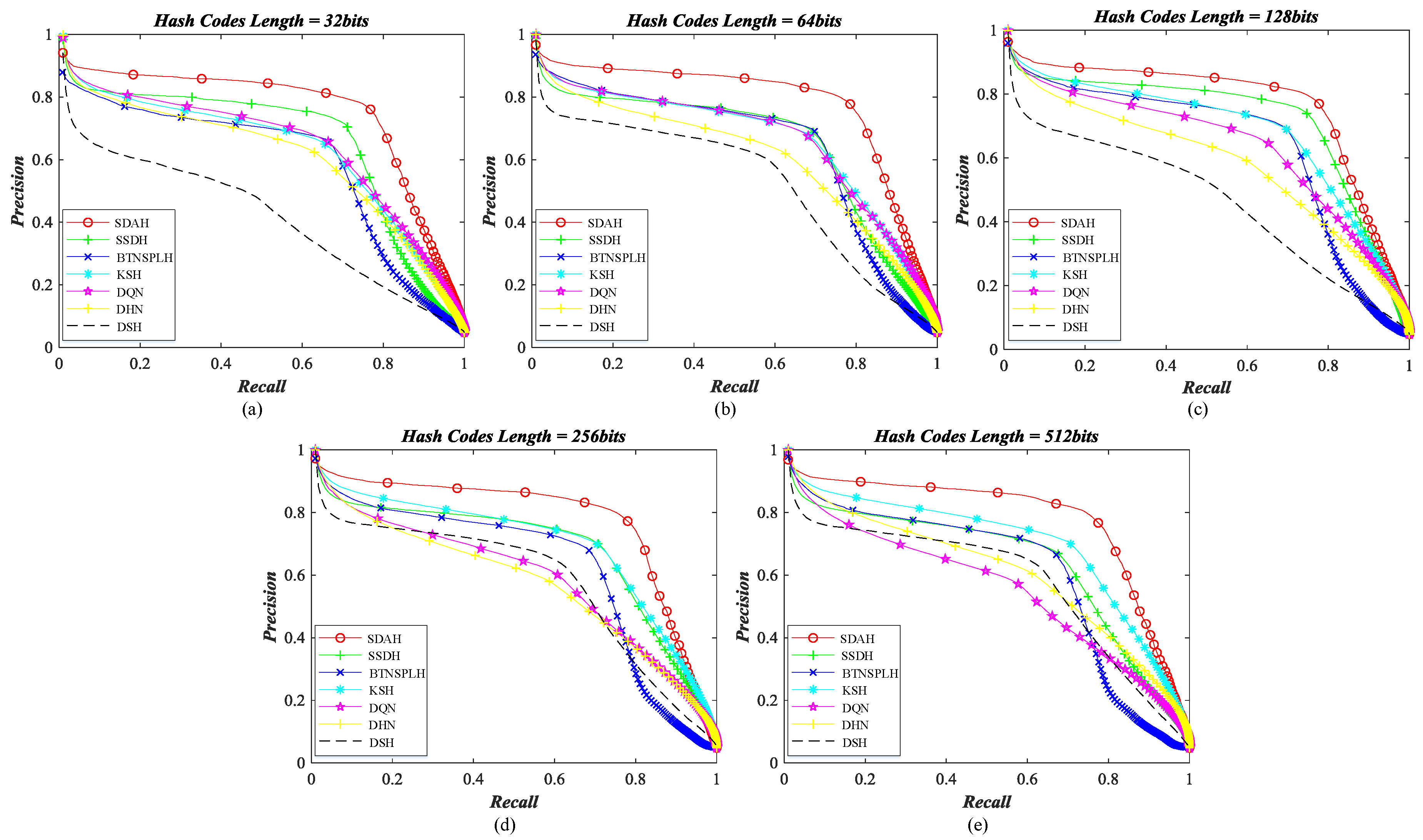
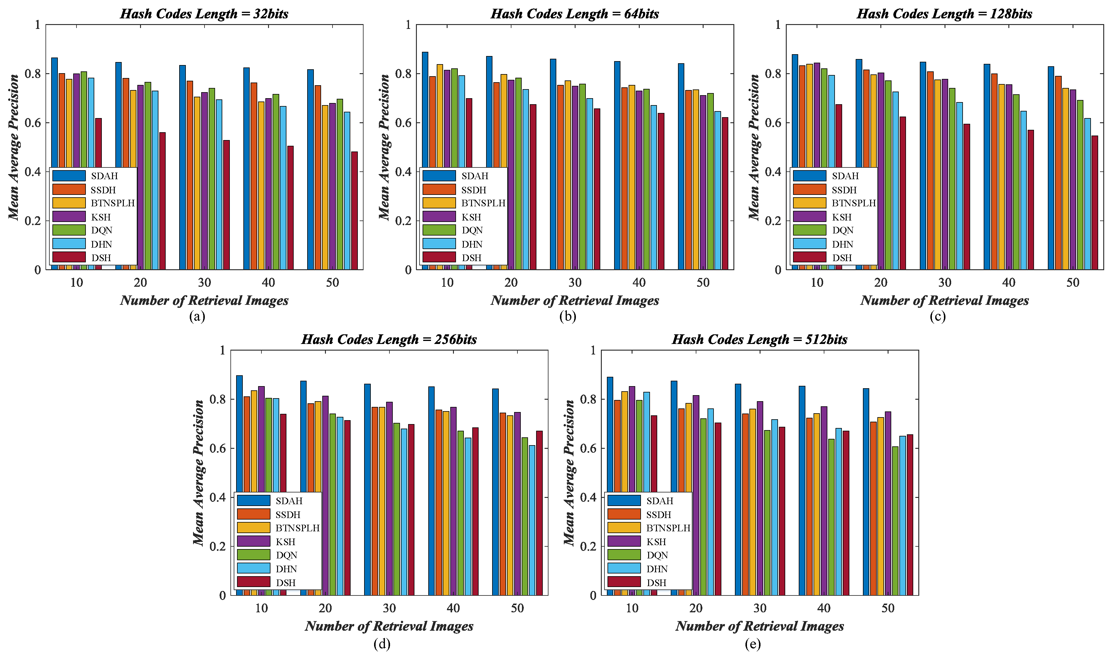
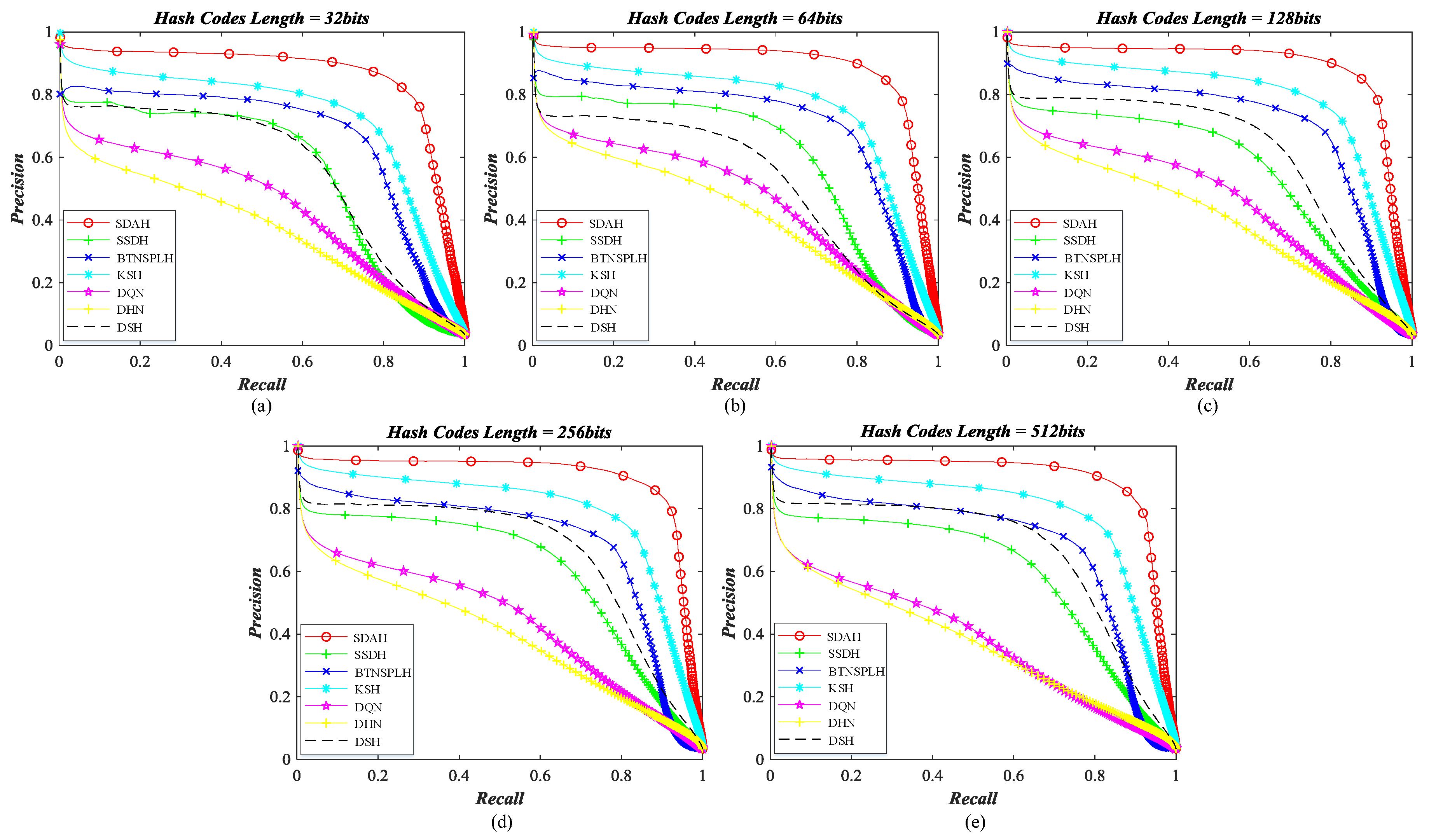
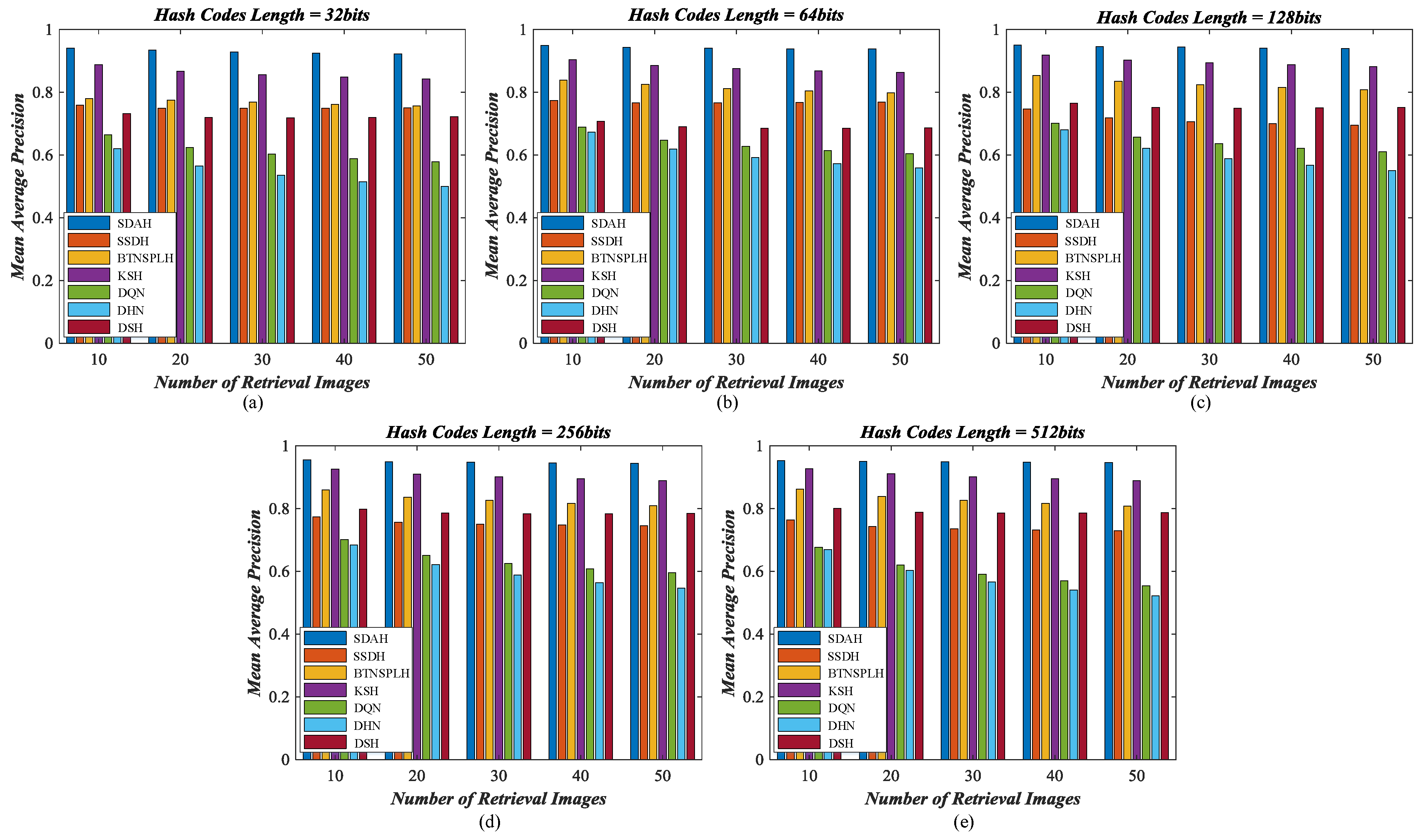
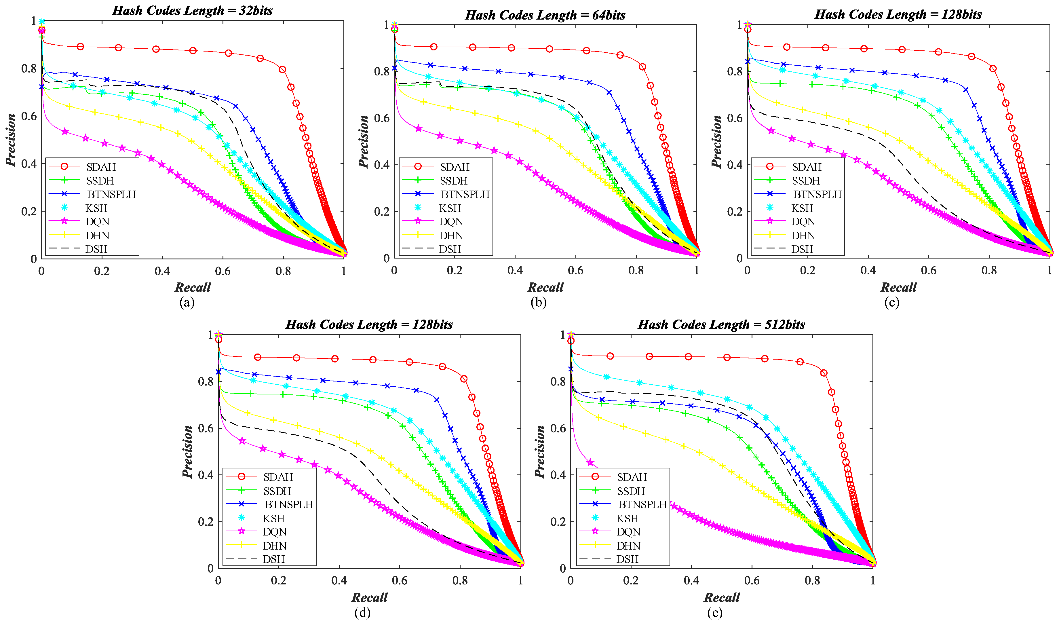
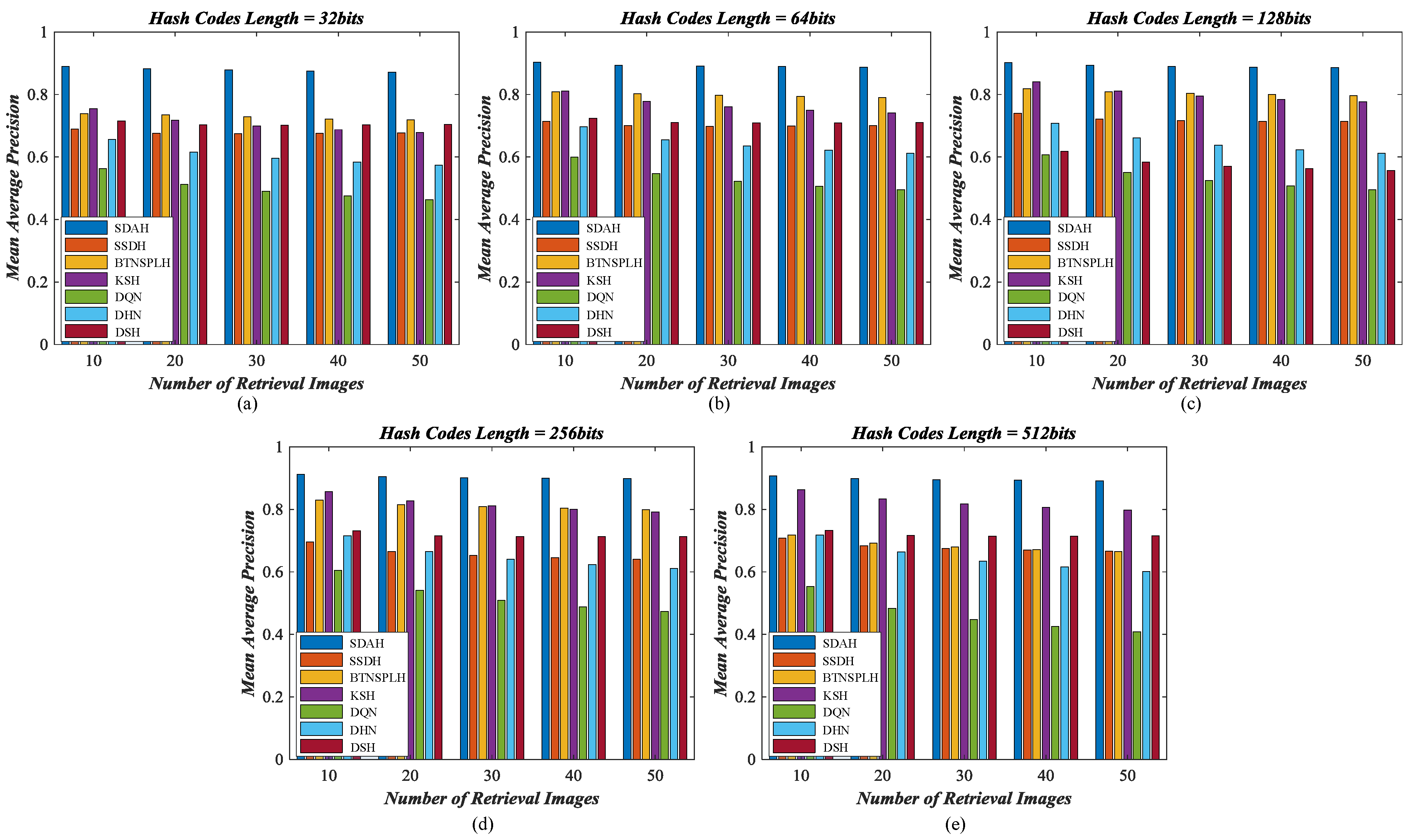
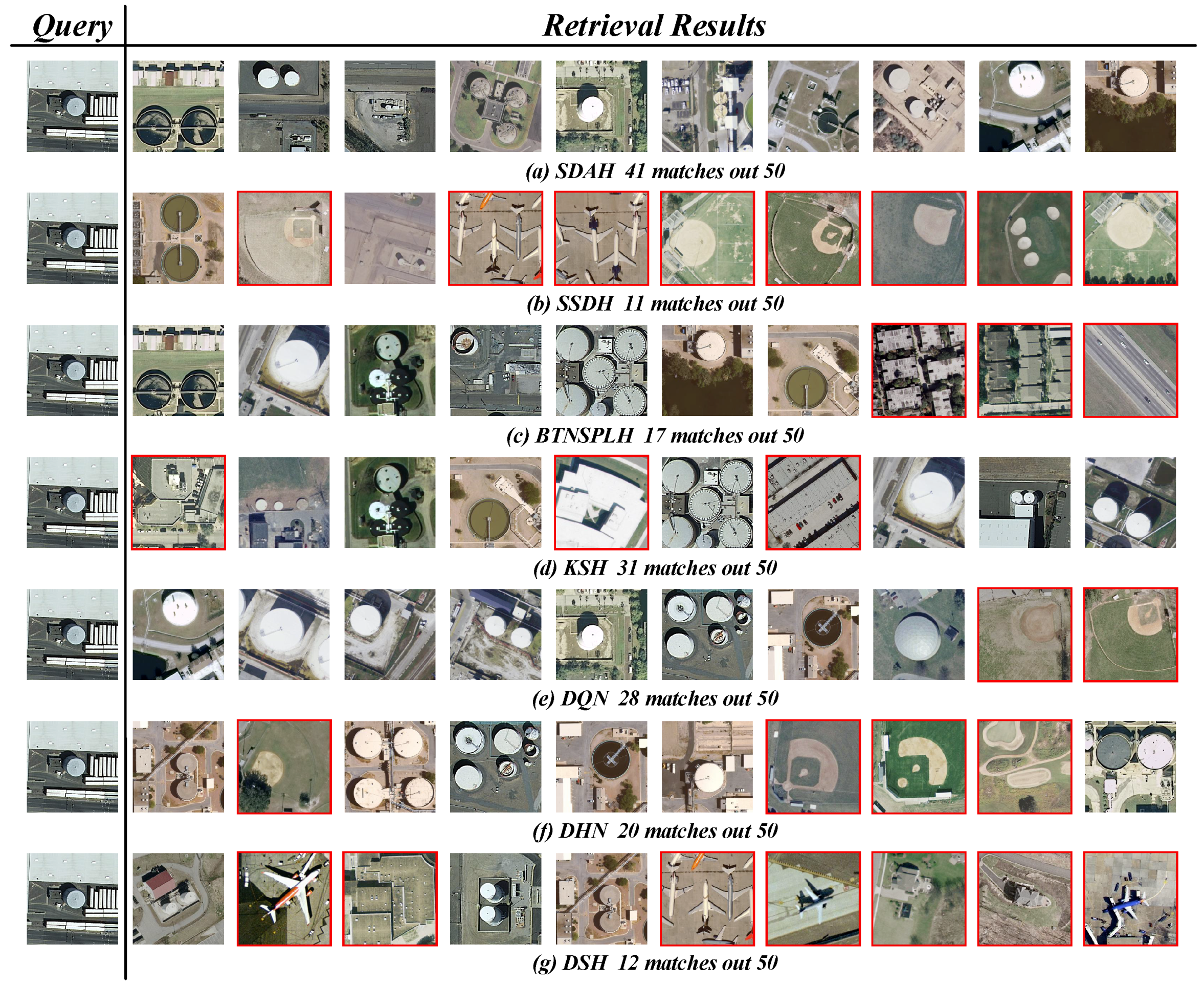
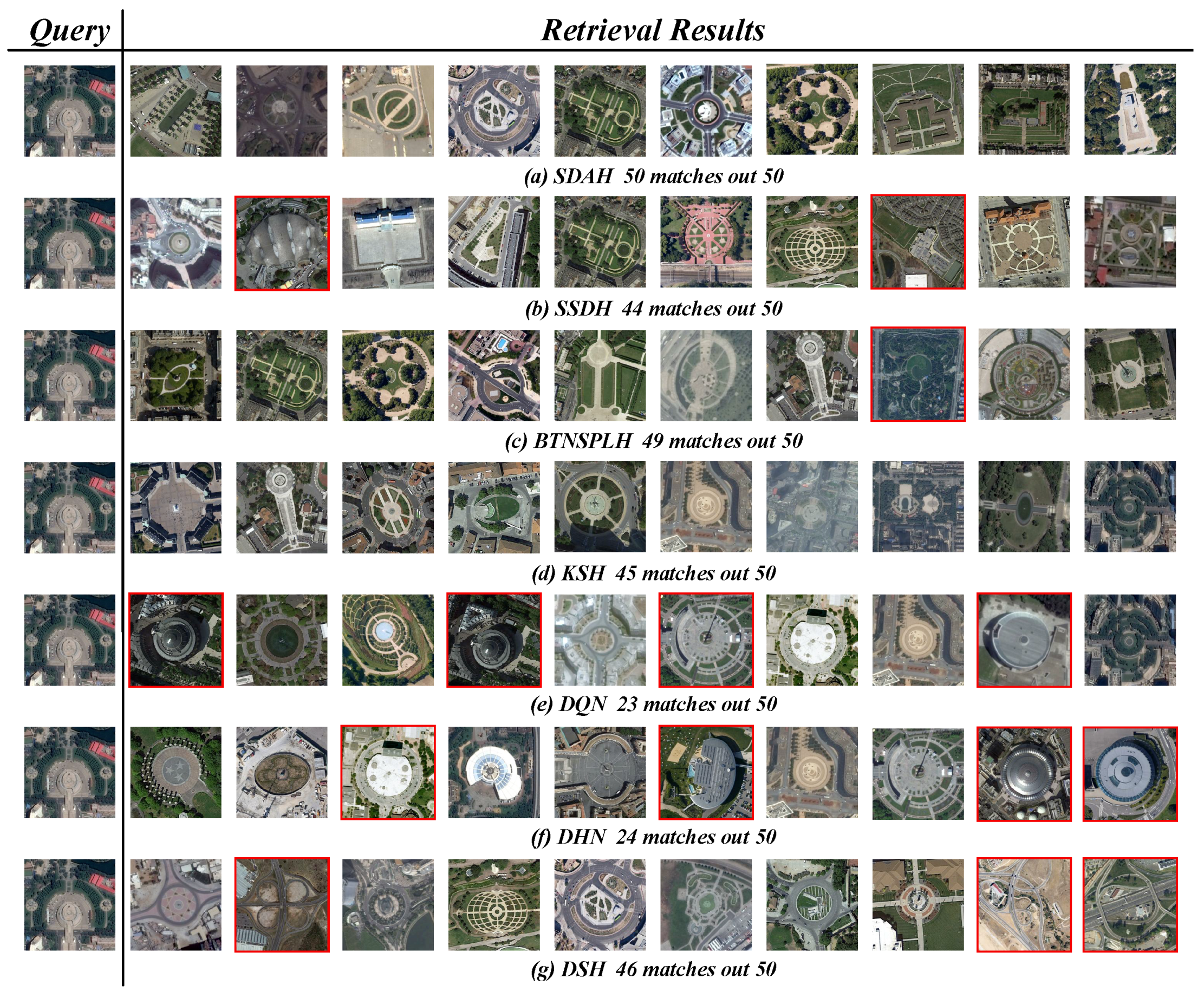
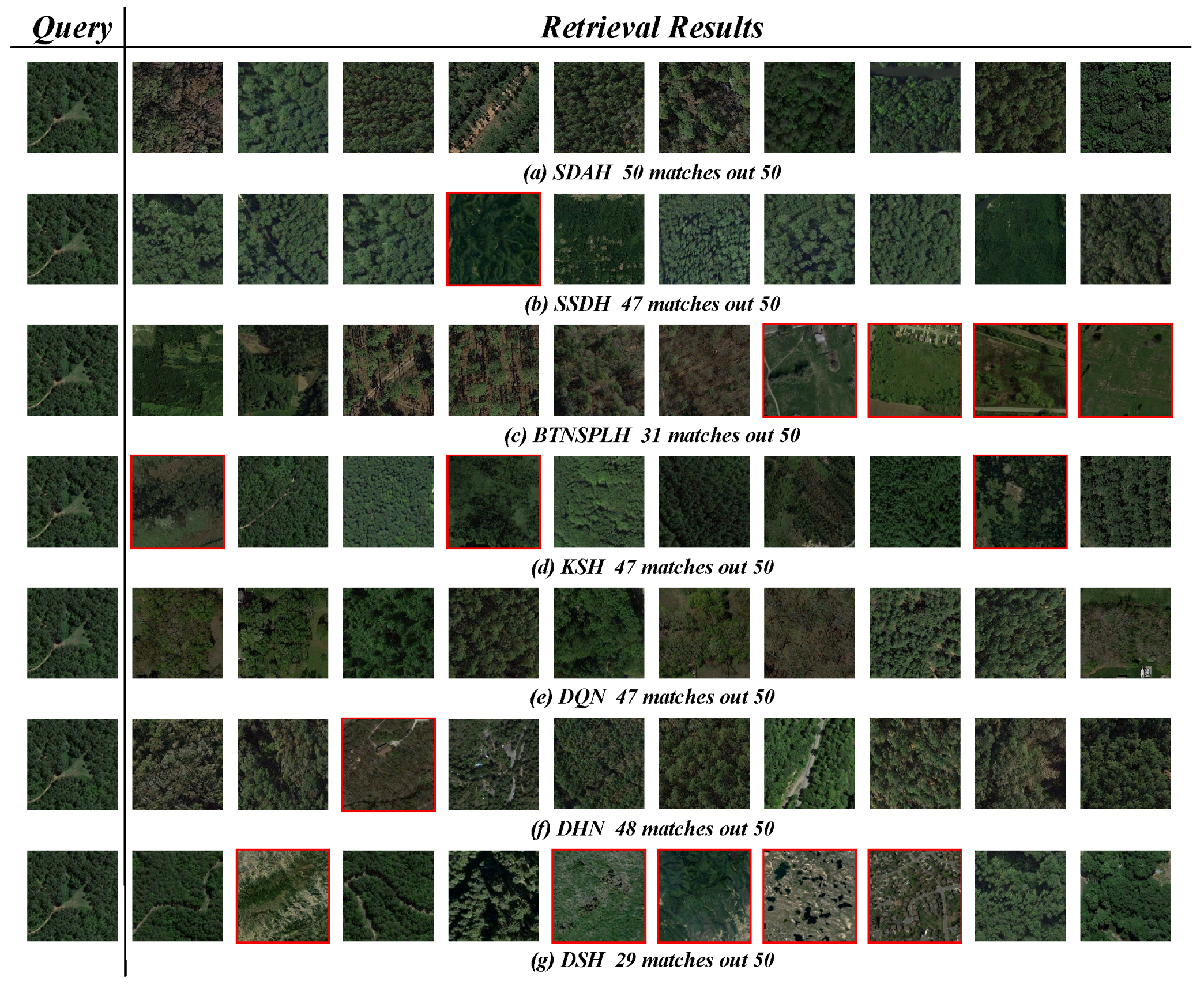
5.3. Retrieval Behavior Compared with Diverse Hashing Methods

To study the performance of our SDAH deeply, we selected six popular hash learning methods for comparison:

• Kernel-based supervised hashing (KSH) [59]. KSH is a classical and successful hash learning method, which aims to map images into the compact binary codes by minimizing/maximizing the hamming distances between similar/dissimilar data pairs. The target hash functions and their algebra relaxation are formulated in the kernel version.
• Bootstrap sequential projection learning based hashing (BTNSPLH) [77]. BTNSPLH develops a nonlinear function for hash learning, which can also explore the latent relationships between images. Meanwhile, a semi-supervised optimization method based on the bootstrap sequential projection learning is proposed to obtain the binary vectors with the lowest errors during the hash coding.
• Semi-supervised deep hashing (SSDH) [78]. SSDH proposes a semi-supervised deep neural network to accomplish the hash leaning in the end-to-end fashion. The developed hashing function minimizes the empirical error on both labeled and unlabeled data, which can preserve the semantic similarities and capture underlying data structures simultaneously.
• Deep quantization network (DQN) based hashing [79]. DQN embeds a hash layer on the top of the normal CNN model to learn the image’s representation and hash codes at the same time. To obtain the useful hash codes, the pairwise cosine loss is developed to remain the similarity relationships between images while the product quantization loss is introduced to reduce the quantization errors.
• Deep hashing network (DHN) [38]. Similar to DQN, another deep neural network with the hashing layer is developed. DHN also develops the specific loss functions to deal with the issues of similarity preserving and quantization loss.
• Deep supervised hashing (DSH) [35]. Based on the usual CNN framework, DSH devises a new hashing network to generate the high discriminative hash codes. Besides preserving the similarity relationships using the supervised information, the designed hash function can also reduce the information loss in the binarization stage by imposing the regularization on the real-valued outputs.

Among the comparison methods, KSH and BTNSPLH are the non-deep hashing techniques, while others are the deep hashing methods. In addition, BTNSPLH and SSDH are semi-supervised models and others are supervised algorithms. All of the approaches were accomplished by the codes published by the authors except SSDH. The parameters were set according to the original literature. Note that, to be fair, the proportion of the training to testing set was 2:8 for all methods. Moreover, the training iteration was set to 50. The experimental results based on different hashing methods are exhibited in Figure 8, Figure 9, Figure 10, Figure 11, Figure 12 and Figure 13.

For UCM dataset, the P-R curves of different hashing methods are exhibited in Figure 8, and the MAPs of diverse hash learning approaches counted by different number of retrieval results are shown in Figure 9. From the observation of figures, we can find that the performance of all hashing models is acceptable, and the hash codes generated by our SDHA outperform others in all scenarios. When the bit of the hash codes is less than 128, the performance of DSH is the weakest. This is because the training data for DSH is limited. As a deep supervised hashing method, DSH needs abundant samples to guarantee its performance. Nevertheless, we only have 420 labeled images (20% of total data), which are not enough for the DSH model, thus its behavior is not as good as expected. The same phenomenon also appears on DHN and DQN models. Their performance is weaker than other compared methods, especially when the bits increases. In contrast, another supervised method, KSH, performs better in most cases. The reason for this is that KSH is a non-deep model, which does not need a large number of training samples to ensure its behavior. The performance of KSH is even better than that of two semi-supervised comparison methods when the length of binary codes equals 512, which illustrates its effectiveness. For BTNSPLH and SSDH, their behavior is better than that of the supervised ones in most situations. This is because not only the supervised information but also the data structure is used to train the models. In addition, the performance of SSDH is stronger than that of BTNSPLH, which demonstrates that the deep hashing is more suitable for UCM dataset. Although the comparison mehods’ behavior is positive, our SDAH can achieve better performance. Taking 128 bits hash codes as the examples, the highest improvements of retrieval precision resulted from our model are 4.64% (SSDH), 8.87% (BTNSPLH), 8.95% (KSH), 13.47% (DQN), 19.12% (DHN), and 26.98% (DSH), while the largest enhancements of retrieval recall achieved by SDAH are 3.46% (SSDH), 10.40% (BTNSPLH), 8.26% (KSH), 12.57% (DQN), 17.97% (DHN), and 26.00% (DSH). Meanwhile, the biggest promotions of retrieval MAP achieved by SDAH are 4.56% (SSDH), 8.79% (BTNSPLH), 9.42% (KSH), 13.73% (DQN), 21.11% (DHN), and 28.26% (DSH).

For the AID archive, the P-R curves of diverse hashing algorithms are shown in Figure 10, and their MAPs counted on a different number of retrieval results are shown displayed in Figure 11. Among the comparison methods, the behavior of DHN and DQN is weaker than others. The performance of DSH and SSDH is close. When the bit length less than 64, SSDH outperforms DSH. Otherwise, the behavior of DSH is better than that of SSDH. A noticed observation is that the performance of DSH increases dramatically when the binary codes get longer, which demonstrates that this deep supervised hashing method needs long bit hash code to ensure its behavior for the AID dataset. Two non-deep hashing approaches, BTNSPLH and KSH, outperform other comparison methods. This is an interesting observation. The reason for this issue is that the iteration times for the deep models are not enough. We believe that the performance of deep models can be enhanced with the increasing iterations. However, time costs may be too large to accept. Compared with the hashing methods discussed above, our model achieves the best performance in all cases. Taking the hash codes with 128 bits as the examples, the largest enhancements of retrieval precision caused by SDAH are 25.83% (SSDH), 14.57% (BTNSPLH), 9.06% (KSH), 35.54% (DQN), 42.15% (DHN), and 20.64% (DSH), while the biggest growth of retrieval recall achieved by SDAH is 26.27% (SSDH), 14.12% (BTNSPLH), 9.51% (KSH), 35.55% (DQN), 41.08% (DHN), and 21.72% (DSH). Meanwhile, the highest promotions of retrieval MAP achieved by SDAH are 24.38% (SSDH), 13.11% (BTNSPLH), 5.75% (KSH), 32.93% (DQN), 38.95% (DHN), and 19.45% (DSH).

For the NWPU archive, the P-R curves of different hashing methods are exhibited in Figure 12, and the MAPs of diverse hash learning approaches counted by different number of retrieval results are shown in Figure 13. We can find a similar conclusion, i.e., our SDAH model achieves the best performance compared with all comparison methods. For non-deep comparison methods, the behavior of BTNSPLH is stronger than that of KSH when the length of hash codes is 32, 64, 128, and 256 bits. Furthermore, the performance of KSH is improved as the code length increases. When the length of hash codes is 512, KSH outperforms BTNSPLH. This indicates that the KSH can achieve positive results as long as the length of generated codes is large enough. For deep comparison methods, the behavior of SSDH is stronger than that of DQH and DHN and is a little weaker than that of DSH. This demonstrates that both of the supervised knowledge and the data structure can help the hashing model to learn the useful hash code. Similar to the AID dataset, the non-deep models outperform the deep models in most cases. The reason for this is that the volume of images within AID and NWPU is relatively large. Deep models should be trained further to reach better performance. However, this would result in much more time costs. Compared with the other methods, the best retrieval results can be obtained using the hash codes learned by our SDAH model. In addition, let us take the hash codes with 128 bits as the examples; the highest enhancements of retrieval precision resulted from our model are 21.07% (SSDH), 13.86% (BTNSPLH), 18.78% (KSH), 44.27% (DQN), 33.05% (DHN), and 36.44% (DSH), while the largest improvements of retrieval recall achieved by SDAH are 20.26% (SSDH), 9.08% (BTNSPLH), 17.85% (KSH), 41.63% (DQN), 30.87% (DHN), and 34.83% (DSH). Meanwhile, the biggest promotions of retrieval MAP achieved by SDAH are 17.30% (SSDH), 8.93% (BTNSPLH), 10.93% (KSH), 39.09% (DQN), 27.38% (DHN), and 32.84% (DSH).

The encouraging results discussed above prove that our method is effective for RS image retrieval. To further study the SDAH model, we count the MAP values across the diverse semantic categories within three datasets using the Top 50 retrievals, and the results are summarized in

Table 7. Retrieval Mean average precision of different hash learning methods across 21 semantic categories in UCM archive counted by Top 50 results. The retrieval results are obtained by the hash codes with 128 bits. The values in bold mean that highest mean average precision of different methods.

	SDAH	SSDH	BTNSPLH	KSH	DQN	DHN	DSH
Agriculture	0.9487	0.9416	0.9349	0.9304	0.9386	0.9376	0.7457
Airplane	0.9438	0.8373	0.8191	0.8510	0.9245	0.9340	0.4622
Baseball Diamond	0.8931	0.9313	0.9378	0.8197	0.9050	0.8597	0.6699
Beach	0.9497	0.9952	0.9955	0.9607	0.9647	0.9303	0.9383
Buildings	0.6772	0.5353	0.7938	0.3125	0.2699	0.3037	0.3152
Chaparral	0.9723	0.9654	0.9451	0.9685	0.9611	0.9562	0.7813
Dense Residential	0.4796	0.3436	0.1834	0.2533	0.1522	0.1645	0.2382
Forest	0.9487	0.9902	0.9700	0.9973	0.9803	0.9442	0.8299
Freeway	0.9642	0.8115	0.6650	0.8253	0.7518	0.5310	0.4530
Golf Course	0.7673	0.6357	0.7634	0.6226	0.6445	0.5373	0.4514
Harbor	0.9452	0.9233	0.7023	0.9747	0.8725	0.7559	0.8240
Intersection	0.7813	0.7696	0.7787	0.5906	0.4692	0.3567	0.5202
Medium-density Residential	0.8182	0.5740	0.5877	0.7210	0.4176	0.3805	0.3175
Mobile Home Park	0.7295	0.7157	0.6530	0.5304	0.5477	0.4064	0.4911
Overpass	0.8070	0.8017	0.7314	0.6044	0.5313	0.3983	0.6388
Parking Lot	0.9436	0.9809	0.4928	0.9824	0.9730	0.8294	0.7406
River	0.8102	0.7906	0.7210	0.6256	0.5285	0.4558	0.4457
Runway	0.9188	0.9099	0.8665	0.9146	0.8282	0.6644	0.8025
Sparse Residential	0.8842	0.8072	0.9641	0.7247	0.6282	0.6098	0.4173
Storage Tanks	0.5743	0.5643	0.2403	0.5059	0.5387	0.4735	0.2197
Tennis Courts	0.6434	0.4696	0.7879	0.6373	0.5588	0.5184	0.1638
Average	0.8286	0.7759	0.7397	0.7311	0.6851	0.6166	0.5460

,

Table 8. Retrieval Mean average precision of different hash learning methods across 30 semantic categories in AID archive counted by Top 50 results. The retrieval results are obtained by the hash codes with 128 bits. The values in bold mean that highest mean average precision of different methods.

	SDAH	SSDH	BTNSPLH	KSH	DQN	DHN	DSH
Airport	0.9661	0.5831	0.8448	0.9403	0.3597	0.4588	0.6298
Bare Land	0.9873	0.7902	0.6731	0.9842	0.3624	0.5352	0.8339
Baseball Field	0.9771	0.8307	0.8910	0.9804	0.5775	0.4645	0.8126
Beach	0.9562	0.7687	0.9680	0.9653	0.8312	0.7224	0.8459
Bridge	0.9649	0.7765	0.9339	0.9632	0.8186	0.7168	0.8117
Center	0.9098	0.6577	0.7360	0.5305	0.2414	0.3002	0.7136
Church	0.9126	0.5572	0.7094	0.8153	0.2017	0.2519	0.6206
Commercial	0.9379	0.4750	0.7527	0.9271	0.3041	0.2671	0.6330
Dense Residential	0.9827	0.6908	0.9288	0.9784	0.7900	0.6719	0.7718
Desert	0.9651	0.8194	0.5360	0.9344	0.4661	0.5230	0.8857
Farmland	0.9481	0.6925	0.9402	0.9520	0.8535	0.7893	0.6895
Forest	0.9717	0.9183	0.8995	0.9566	0.8876	0.8631	0.9263
Industrial	0.9353	0.5745	0.7946	0.9129	0.4837	0.3854	0.6467
Meadow	0.9707	0.9188	0.8049	0.9691	0.8213	0.8295	0.9186
Medium Residential	0.9281	0.6719	0.7780	0.8668	0.4677	0.4404	0.6896
Mountain	0.9686	0.7784	0.9675	0.9600	0.8929	0.7606	0.8622
Park	0.8884	0.5717	0.3321	0.6658	0.1991	0.2667	0.6503
Parking	0.9894	0.9116	0.9436	0.9763	0.9946	0.9459	0.9513
Playground	0.9502	0.7330	0.9309	0.9704	0.7496	0.6440	0.7991
Pond	0.9254	0.6867	0.8809	0.9693	0.7867	0.5993	0.7784
Port	0.9648	0.7400	0.8018	0.9642	0.5954	0.5181	0.7700
Railway Station	0.9087	0.5789	0.8138	0.8120	0.4146	0.3852	0.6367
Resort	0.8493	0.4789	0.5710	0.4257	0.1178	0.1069	0.5182
River	0.9646	0.6312	0.8880	0.9628	0.6448	0.3307	0.6979
School	0.7914	0.3656	0.6237	0.6386	0.1042	0.1127	0.3917
Sparse residential	0.9828	0.8575	0.9724	0.9798	0.9227	0.8608	0.8533
Square	0.8582	0.3666	0.4750	0.3565	0.1937	0.1285	0.5231
Stadium	0.9541	0.8922	0.9382	0.9780	0.8740	0.7585	0.9034
Storage tanks	0.8767	0.7668	0.7632	0.8741	0.8134	0.5935	0.8577
Viaduct	0.9958	0.8023	0.9390	0.9846	0.9793	0.9370	0.8550
Average	0.9394	0.6962	0.8011	0.8732	0.5917	0.5389	0.7493

and

Table 9. Retrieval Mean average precision of different hash learning methods across 45 semantic categories in NMPU archive counted by Top 50 results. The retrieval results are obtained by the hash codes with 128 bits. The values in bold mean that highest mean average precision of different methods.

	SDAH	SSDH	BTNSPLH	KSH	DQN	DHN	DSH
Airplane	0.9264	0.8064	0.9258	0.8801	0.6249	0.7801	0.7700
Airport	0.8661	0.5673	0.3985	0.6475	0.2310	0.4976	0.2910
Baseball Diamond	0.9259	0.7089	0.9470	0.8753	0.2754	0.4615	0.5786
Basketball Court	0.8508	0.5391	0.9312	0.5563	0.1251	0.3489	0.4095
Beach	0.9381	0.7883	0.8797	0.8549	0.4300	0.6506	0.5875
Bridge	0.8905	0.7999	0.9525	0.8708	0.6461	0.7402	0.6834
Chaparral	0.9754	0.9689	0.9384	0.9667	0.9391	0.9447	0.7546
Church	0.7778	0.4859	0.6902	0.3849	0.0706	0.2138	0.2426
Circular Farmland	0.9516	0.8773	0.9125	0.9241	0.9091	0.9270	0.7249
Cloud	0.9723	0.9232	0.9728	0.9711	0.9519	0.9347	0.9370
Commercial Area	0.7857	0.4903	0.8125	0.4987	0.1928	0.4174	0.3659
Dense Residential	0.8434	0.6357	0.8755	0.7972	0.3967	0.4670	0.3909
Desert	0.9383	0.8891	0.8939	0.9001	0.8394	0.8425	0.8296
Forest	0.9486	0.8668	0.5751	0.9332	0.8569	0.8289	0.6403
Freeway	0.8778	0.5866	0.7960	0.5119	0.3270	0.3471	0.4567
Golf Course	0.8735	0.7455	0.9145	0.8255	0.6063	0.7205	0.6424
Ground Track Field	0.9170	0.6986	0.9046	0.9094	0.2855	0.4943	0.6375
Harbor	0.9534	0.8231	0.8851	0.8970	0.7680	0.8096	0.6062
Industrial Area	0.8811	0.6543	0.5709	0.7620	0.5537	0.6051	0.4530
Intersection	0.8843	0.7279	0.8414	0.8160	0.3174	0.6676	0.6722
Island	0.9335	0.8925	0.8758	0.9227	0.7559	0.7886	0.8098
Lake	0.9291	0.8056	0.8137	0.8394	0.7151	0.7447	0.7410
Meadow	0.9376	0.8690	0.4655	0.8756	0.7802	0.7495	0.7957
Medium Residential	0.7869	0.5356	0.6655	0.5448	0.2460	0.3478	0.2664
Mobile Home Park	0.8670	0.7240	0.9051	0.8599	0.2915	0.5411	0.5180
Mountain	0.9021	0.7057	0.8992	0.8381	0.6495	0.6674	0.2659
Overpass	0.9403	0.7429	0.9022	0.8205	0.4358	0.6185	0.5801
Palace	0.6588	0.4539	0.5326	0.2617	0.0659	0.1053	0.2487
Parking Lot	0.9466	0.7914	0.8986	0.8985	0.5695	0.7066	0.7377
Railway	0.8916	0.6106	0.7079	0.7709	0.4158	0.4429	0.5240
Railway Station	0.8418	0.6499	0.2873	0.6035	0.1968	0.3925	0.4480
Rectangular Farmland	0.8750	0.6560	0.7838	0.8194	0.6961	0.7155	0.3041
River	0.8336	0.5890	0.7924	0.5617	0.3015	0.4767	0.3939
Roundabout	0.8343	0.7346	0.9212	0.8879	0.6344	0.7619	0.6350
Runway	0.8465	0.7236	0.7872	0.7054	0.3776	0.5210	0.6405
Sea Ice	0.9812	0.9467	0.9795	0.9606	0.9085	0.9146	0.9311
Ship	0.8679	0.5999	0.9194	0.8160	0.2772	0.6068	0.4182
Snowberg	0.9553	0.8950	0.9369	0.9447	0.9071	0.8867	0.7867
Sparse Residential	0.9285	0.6838	0.3809	0.8631	0.3858	0.6606	0.4903
Stadium	0.8854	0.7499	0.8782	0.8302	0.6231	0.6526	0.7206
Storage Tank	0.9184	0.7841	0.8226	0.7864	0.6635	0.7739	0.6866
Tennis Court	0.7918	0.4402	0.8991	0.6653	0.0959	0.1987	0.2357
Terrace	0.8542	0.6699	0.7217	0.8051	0.3727	0.5907	0.3062
Thermal Power Station	0.8513	0.6147	0.8334	0.7251	0.2971	0.5558	0.5132
Wetland	0.8116	0.6574	0.5818	0.5126	0.2484	0.4064	0.3991
Average	0.8855	0.7135	0.7958	0.7756	0.4946	0.6117	0.5571

. From the observation of tables, we can easily find that the proposed method performs best in most of the categories. For the UCM archive, compared with other hashing methods, the highest enhancements achieved by SDAH appear in “Medium-density Residential” (SSDH, DHN), “Parking Lot” (BTNSPLH), “Buildings” (KSH, DQN), and “Freeway” (DSH). For the AID archive, the largest improvements of our model appear in “Commercial” (SSDH), “Park” (BTNSPLH), “Square” (KSH), “Resort” (DQN, DHN), and “School” (DSH). For the NWPU dataset, the biggest superiority of our method can be found in “Tennis Court” (SSDH, DHN), “Railway Station” (BTNSPLH), “Palace” (KSH), “Basketball Court” (DQN), and “Mountain” (DSH). Moreover, an encouraging observation is that SDAH remains relatively high performance in some categories which other comparison methods’ behavior is unsatisfactory, such as “Dense Residential” (UCM), “Resort” (AID) and “River” (NWPU). It is worth noting that our SDAH cannot achieve the best retrieval results on a few of categories, such as “Baseball Diamond” (UCM), “Pond” (AID) and “Bridge” (NWPU). Nevertheless, its behavior remains in the Top 2 position, which demonstrates the proposed method performs steadily. These favorable results illustrate the usefulness of the proposed method again.

Apart from the numerical assessment, we also study the structure of the learned hash codes using the t-distributed stochastic neighbor embedding (t-SNE) algorithm [80] in this part. In addition, the structure of the hash codes obtained by the comparison methods is provided for reference. Here, the hamming distance is selected to complete the t-SNE algorithm, and the hash codes’ dimension is reduced from 128 to 2. The visual results of different hash codes are exhibited in Figure 14, Figure 15 and Figure 16. From the observation of the figures, we can easily find that the structure of the hash codes learned by our SDAH model (Figure 14a and Figure 15a) is the clearest among all of the results, in which the clusters are obviously separable and the distances between different clusters are distinct. For the comparison methods, similar to the numerical analysis, the results of non-deep hashing (KSH and BTNSPLH) are better than those of deep hashing (DQH, DHN, and DSH), and the results of the semi-supervised hashing (SSDH and BTNSPLH) is better than those of the supervised hashing (DQH, DHN, and DSH) in general. These positive results prove the effectiveness of our model again.

We also display some retrieval examples obtained by different hashing methods in Figure 17, Figure 18 and Figure 19. Here, we adopted the 128 bits hash codes learned by diverse hashing methods and hamming distance metric to obtain the retrieval results. Three RS images were randomly picked up from three archives, which belong to “Storage Tanks” (UCM), “Square” (AID) and “Forest” (NWPU), respectively. Due to the space limitation, only the Top 10 retrieval images are exhibited. The first images within each row are the queries, and then the retrieval results are listed according to the hamming distances’ order. The incorrect results are tagged in red for clarity. In addition, the number of correct results within the Top 50 retrieval images is also provided for reference. It is obvious that our SDAH performs best. For the “Storage Tanks” query, the Top 10 results obtained by SDAH are totally correct, and there are only nine incorrect results within the Top 50 results. For the “Square” and the “Forest” queries, the Top 50 retrieval results obtained by our model are totally correct.

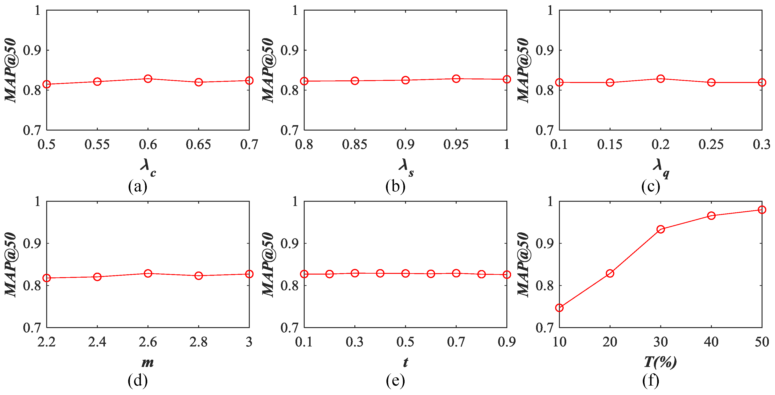
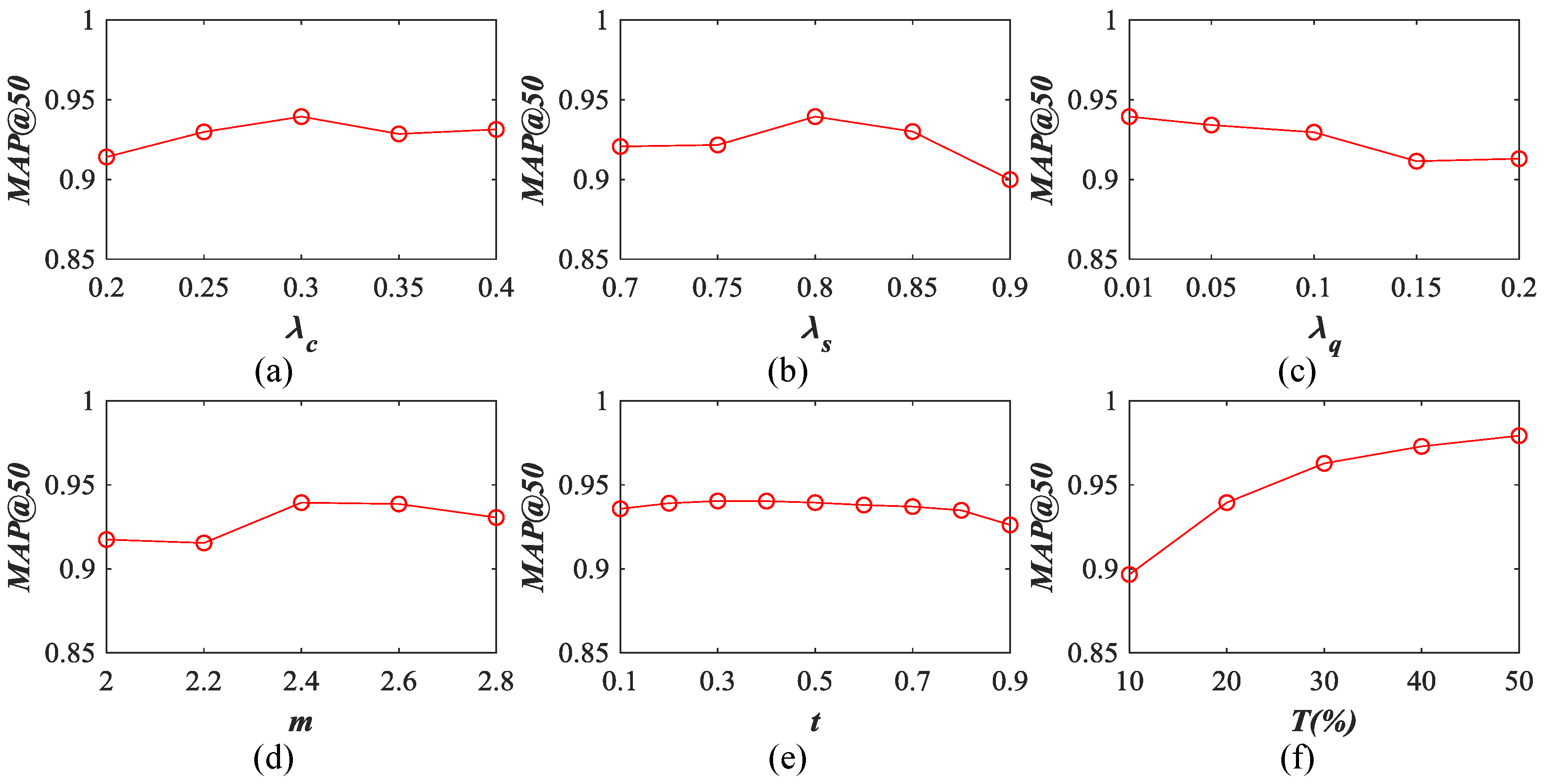
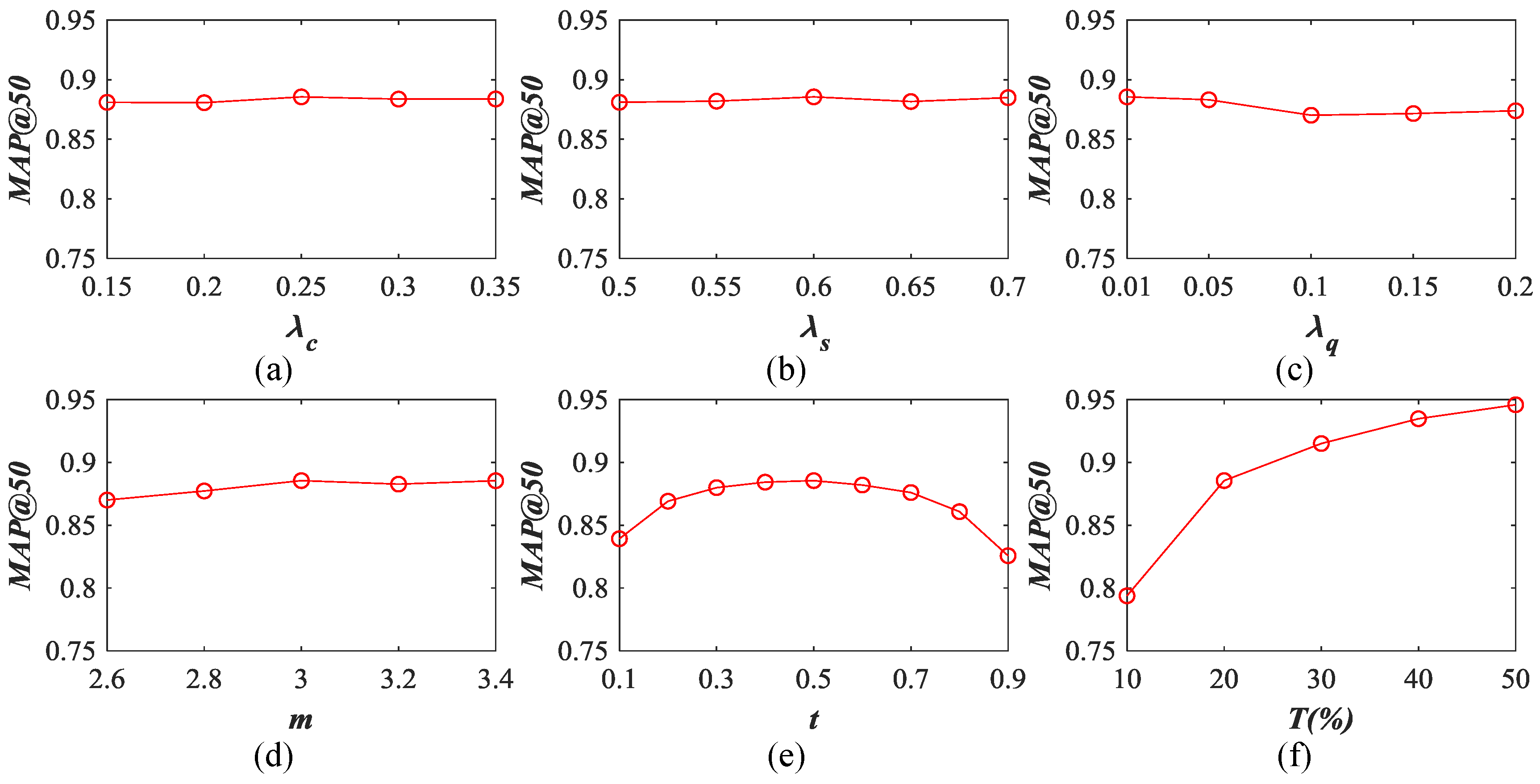
5.4. Influence of Different Parameters

The influence of different parameters on our SDAH model is discussed in this section. As mentioned in Section 5.2, there are four free parameters within our hashing function (Equation (16)), including three weighting variate ${\lambda }_c$, ${\lambda }_s$ and ${\lambda }_q$, and one margin parameter m. Besides those parameters, there are still two factors that impact our model: the threshold t for the binarization (introduced in Section 3.3.4) and the percentage of the samples T for training SDAH network. To study their influence on our method, we first fixed the length of hash codes to be 128 bits here. Then, we tuned the values of different parameters with certain limits to observe the variation of our method. For the UCM dataset, we set ${\lambda }_c\in \left[0.50,0.70\right]$, ${\lambda }_s\in \left[0.80,1.00\right]$, ${\lambda }_q\in \left[0.10,0.30\right]$, and $m\in \left[2.2,3.0\right]$. For the AID dataset, we set ${\lambda }_c\in \left[0.20,0.40\right]$, ${\lambda }_s\in \left[0.70,0.90\right]$, ${\lambda }_q\in \left[0.01,0.20\right]$, and $m\in \left[2.0,2.8\right]$. For the NWPU archive, we set ${\lambda }_c\in \left[0.15,0.35\right]$, ${\lambda }_s\in \left[0.80,1.00\right]$, ${\lambda }_q\in \left[0.01,0.20\right]$, and $m\in \left[2.6,3.4\right]$. Moreover, the range of the other two parameters was unified as $t\in \left[0.1,0.9\right]$ and $T\in \left[10,50\right]\left(\%\right)$ for the three image databases. Note that only one parameter was changed at one time, and the others were fixed according to Table 5.

The results on the UCM image database using the Top 50 retrieval images are exhibited in Figure 20. From the observation, we found that the free parameters within the hash function (${\lambda }_c$, ${\lambda }_s$, ${\lambda }_q$ and m) impact our SDAH model slightly, which demonstrates that our method is robust to the UCM dataset. In detail, for ${\lambda }_c$, when ${\lambda }_c\le 0.60$ SDAH’s performance is enhanced with the value of ${\lambda }_c$ grows. When ${\lambda }_c>0.60$, the behavior of SDAH is reduced slightly. For ${\lambda }_s$, the whole trend of SDAH’s behavior is upward with the increased ${\lambda }_s$. The peak value appears at ${\lambda }_s=0.95$. For ${\lambda }_q$, the best performance of SDAH can be obtained when ${\lambda }_q=0.20$, and the behavior is affected with small degrees when the ${\lambda }_s$ value is larger or less than 0.20. The results of different m are similar to ${\lambda }_s$. SDAH can reach the peak value when m is equal to 2.6, and the performance is decreased in other cases. For the other two parameters, i.e., the binarization threshold t and the training data percentage T, the following conclusion can be summarized. The performance of SDAH almost remains with the varied t, which indicates that our method is not sensitive to t. Furthermore, it also means that the elements within vectors before the binarization are close to 0 or 1, which demonstrates the superiority of our model. For training data percentage T, it is obvious that better performance can be achieved with more training data. However, more training data would result in larger time costs. Thus, in this study, we kept the percentage of the training data at 20%.

The results counted on the AID dataset using the Top 50 retrieval images are shown in Figure 21. For ${\lambda }_c$, the peak value appears at ${\lambda }_c=0.3$. When ${\lambda }_c<0.3$, the SDAH’s performance is increasing. When ${\lambda }_c>0.3$, the performance of SDAH first goes down and then goes up. For ${\lambda }_s$, the best behavior can be obtained when ${\lambda }_s=0.8$. Otherwise, SDAH’s performance is decreased more or less. For ${\lambda }_q$, the performance of SDAH is decreasing when the value of ${\lambda }_q$ grows. For m, when $m<2.4$, the model’s performance is ascending and the peak value appears at $m=2.4$. When $m>2.4$, the behavior of SDAH falls slightly. Although the above four parameters impact our model at different levels, their influence remains in an acceptable range. Similar to the UCM dataset, the performance of SDAH varies within a narrow range with different t. This means that the outputs of our model are the binary-like vectors, which proves the usefulness of our SDAH for hash learning. For T, it is obvious that more training data leads to better performance. Taking the time consumption into account, we kept $T=20\%$.

The results on the NWPU image archive using the Top 50 retrieval images are exhibited in Figure 22. Similar to the results of other two datasets, the impact of ${\lambda }_c$, ${\lambda }_s$, ${\lambda }_q$ and m on SDAH is not drastic. The SDAH’s performance peak values appear at ${\lambda }_c=0.25$, ${\lambda }_s=0.60$, ${\lambda }_q=0.01$, and $m=3.0$. When their values change, the behavior of SDAH fluctuates in a small range. In addition, for training data percentage T, we can find the same results, i.e., the larger training data the better performance. To keep the trade-off between training time costs and performance, we chose $T=20\%$ for NWPU. An interesting observation is that our model is sensitive to the binarization threshold t for NWPU. The weakest performance is 0.8257 when $t=0.9$ while the strongest behavior is 0.8856 when $t=0.5$. The reason for this is that the elements of the vectors before the binarization are not close enough to 0 or 1, which indicates that our model still has the space for the enhancement.

5.5. Computational Cost

In this section, we discuss the computational cost of our model from the following aspects, including the time cost of hash learning and the retrieval efficiency.

The time cost of hash learning can be divided into two parts, i.e., SDAH network training and hash codes generation. For model training, the time costs depend on the volume of the training set directly. Suppose we still select 20% images from the archive to construct the training set. Thus, the numbers of training data corresponding to different archives are 420 (UCM), 2000 (AID), and 6300 (NWPU). In addition, as mentioned in Section 5.2, we chooe AlexFineFC7 as the input visual feature. Therefore, the dimension of the training data was fixed to 4096. Under these conditions, we need around 6 min (UCM), 15 min (AID), and 25 min (NWPU) to accomplish the network training for the 128-bit hash codes. It is noted that the time consumption of model training is similar when the length of hash codes varies between 32 and 512. When the SDAH model is trained, the hash codes generation is fast, needing approximately 0.1 ms for input data.

To deeply study the retrieval speed of SDAH, we changed the archive size and calculated the similarity and ranking time costs under the different lengths of hash codes. In detail, based on the NWPU image dataset, we constructed the target archives with the size of 1000, 5000, 10,000, 15,000, 20,000, 25,000, and 31,500. Then, 300 images were randomly selected to be the queries, and the final retrieval speed was the average value counted on these query images. Meanwhile, the retrieval times based on the original features (AlexFineFC7) are also provided as a reference. Note that the similarities between hash codes were calculated by hamming distance while the resemblance between AlexFineFC7 features was computed by Euclidean distance.

The results are summarized in

Table 10. Retrieval cost of similarity calculation and matching based on original features and hash codes with different length (unit: millisecond).

Target Image Archive Size		1000	5000	10,000	15,000	20,000	25,000	31,500
AlexFineFC7		31.79	152.71	306.00	454.86	563.74	765.99	949.25
Hash codes bits	32	0.60	1.36	2.81	3.14	3.74	5.46	6.25
	64	0.81	2.47	4.23	6.58	7.99	11.03	13.08
	128	1.28	4.76	9.68	13.97	18.09	23.43	29.56
	256	2.41	10.40	21.45	32.78	43.40	54.36	68.28
	512	4.76	22.16	45.70	64.16	79.11	106.32	132.72

. It is obvious that the retrieval based on the hash codes is much faster than the search on the basis of AlexFineFC7 features, especially when the size of the dataset is large. The reasons can be summarized as follows. The AlexFineFC7 features are continuous and dense. To obtain the similarities between these vectors, the distance metric should calculate the differences between every element pairs, which is a time-consuming procedure. Moreover, the dimension of AlexFineFC7 features is 4096, which increases the time costs of similarity computation. In contrast, the hash codes are discrete and their elements are 0 or 1. To measure the resemblance between them, the hamming distance metric only needs to count the number of different element pairs. Furthermore, the dimension of hash codes is low. Consequently, the time costs of similarity matching based on the hash codes are small. The retrieval efficiency results demonstrate that the hash codes are more suitable for the large-scale scenario.

6. Conclusions

Under the paradigm of generative adversarial learning, a new semi-supervised deep hashing method named SDAH is presented in this paper. The generator G of SDAH is the encoder of RAE, which focuses on learning the class variable $\mathbf{y}$ and hash code $\mathbf{b}$ using the input visual features. Two discriminators ($D_c$ and $D_u$) aim to impose the categorical distribution and binary uniform distribution on $\mathbf{y}$ and $\mathbf{b}$, respectively. Through the regularization, the class variable $\mathbf{y}$ could be the approximate one-hot vector that reflects the class information, while the hash code $\mathbf{b}$ could be the bit-balanced vector with the binary-like values. The generator and the discriminators can be trained using the total data with the reconstruction loss function and minimax loss function under the generative adversarial learning framework. Furthermore, to improve the performance of hash code, a specific hashing function is developed. Only a small number of labeled data should be used to optimize the hashing function. Integrating the generator, discriminators, and hashing function optimization together, the discriminative, similarity preserving and low quantization error hash code can be obtained.

We selected three published RS archives (UCM, AID, and NWPU) to verify the usefulness of our SDAH. First, our model can learn the hash codes from different visual features, including the mid-level BOW vectors and the high-level deep vectors (AlexFC7, VGG16FC7, AlexFineFC7, and VGG16FineFC7). In addition, the retrieval performance of learned hash codes is better than that of the original visual features. In general, enhancements of around 10% can be achieved. Second, we compared our SDAH with six other popular hash learning methods (SSDH, BTNSPLH, KSH, DQN, DHN, and DSH). Fixing the input feature (AlexFineFC7) and the length hash codes (128 bits), the MAP values of our SDAH counted on Top 50 retrieval results are 0.8286 (UCM), 0.9394 (AID), and 0.8855 (NWPU), which are higher than those of the comparison methods. Third, the learned hash codes can obviously speed up the retrieval efficiency compared with the original visual features. The promising experimental results counted on different RS image datasets prove that our SDAH is effective to the RSIR task.

References

1. Zhou, W.; Newsam, S.; Li, C.; Shao, Z. PatternNet: A benchmark dataset for performance evaluation of remote sensing image retrieval. ISPRS J. Photogramm. Remote Sens. 2018, 145, 197–209. [Google Scholar] [CrossRef] [Green Version]
2. Quartulli, M.; Olaizola, I.G. A review of EO image information mining. ISPRS J. Photogramm. Remote Sens. 2013, 75, 11–28. [Google Scholar] [CrossRef] [Green Version]
3. Shyu, C.R.; Klaric, M.; Scott, G.J.; Barb, A.S.; Davis, C.H.; Palaniappan, K. GeoIRIS: Geospatial information retrieval and indexing system—Content mining, semantics modeling, and complex queries. IEEE Trans. Geosci. Remote Sens. 2007, 45, 839–852. [Google Scholar] [CrossRef] [PubMed]
4. Aptoula, E. Remote sensing image retrieval with global morphological texture descriptors. IEEE Trans. Geosci. Remote Sens. 2013, 52, 3023–3034. [Google Scholar] [CrossRef]
5. Demir, B.; Bruzzone, L. Hashing-based scalable remote sensing image search and retrieval in large archives. IEEE Trans. Geosci. Remote Sens. 2015, 54, 892–904. [Google Scholar] [CrossRef]
6. Gu, Y.; Wang, Y.; Li, Y. A Survey on Deep Learning-Driven Remote Sensing Image Scene Understanding: Scene Classification, Scene Retrieval and Scene-Guided Object Detection. Appl. Sci. 2019, 9, 2110. [Google Scholar] [CrossRef]
7. Wang, Q.; Chen, M.L.; Nie, F.P.; Li, X.L. Detecting coherent groups in crowd scenes by multiview clustering. IEEE Trans. Pattern Anal. Mach. Intell. 2018. [Google Scholar] [CrossRef]
8. Wang, Q.; Qin, Z.Q.; Nie, F.P.; Li, X.L. Spectral embedded adaptive neighbors clustering. IEEE Trans. Neural Netw. Learn. Syst. 2018, 30, 1265–1271. [Google Scholar] [CrossRef]
9. Wang, Q.; Wan, J.; Li, X.L. Hierarchical feature selection for random projection. IEEE Trans. Neural Networks and Learning Systems 2018, 30, 1581–1586. [Google Scholar] [CrossRef]
10. Wang, Q.; Wan, J.; Nie, F.P.; Liu, B. Robust hierarchical deep learning for vehicular management. IEEE Trans. Veh. Technol. 2018, 68, 4148–4156. [Google Scholar] [CrossRef]
11. Wang, J.; Shen, H.T.; Song, J.; Ji, J. Hashing for similarity search: A survey. arXiv 2014, arXiv:1408.2927. [Google Scholar]
12. Wang, J.; Zhang, T.; Sebe, N.; Shen, H.T. A survey on learning to hash. IEEE Trans. Pattern Anal. Mach. Intell. 2017, 40, 769–790. [Google Scholar] [CrossRef] [PubMed]
13. Muja, M.; Lowe, D.G. Fast approximate nearest neighbors with automatic algorithm configuration. VISAPP 2009, 2, 2. [Google Scholar]
14. Muja, M.; Lowe, D.G. Scalable nearest neighbor algorithms for high dimensional data. IEEE Trans. Pattern Anal. Mach. Intell. 2014, 36, 2227–2240. [Google Scholar] [CrossRef] [PubMed]
15. Indyk, P.; Motwani, R. Approximate nearest neighbors: Towards removing the curse of dimensionality. In Proceedings of the Thirtieth Annual ACM Symposium on Theory of Computing, Dallas, TX, USA, 24–26 May 1998; pp. 604–613. [Google Scholar]
16. Charikar, M.S. Similarity estimation techniques from rounding algorithms. In Proceedings of the Thiry-Fourth Annual ACM Symposium on Theory of Computing, Montreal, QC, Canada, 19–21 May 2002; pp. 380–388. [Google Scholar]
17. Andoni, A.; Indyk, P. Near-optimal hashing algorithms for approximate nearest neighbor in high dimensions. Commun. ACM 2008, 51, 117. [Google Scholar] [CrossRef]
18. Chi, L.; Zhu, X. Hashing techniques: A survey and taxonomy. ACM Comput. Surv. (CSUR) 2017, 50, 11. [Google Scholar] [CrossRef]
19. Gionis, A.; Indyk, P.; Motwani, R. Similarity search in high dimensions via hashing. In Proceedings of the 25rd International Conference on Very Large Data, Edinburgh, Scotland, UK, 7–10 September 1999; pp. 518–529. [Google Scholar]
20. Datar, M.; Immorlica, N.; Indyk, P.; Mirrokni, V.S. Locality-sensitive hashing scheme based on p-stable distributions. In Proceedings of the Twentieth Annual Symposium on Computational Geometry, Brooklyn, NY, USA, 8–11 June 2004; pp. 253–262. [Google Scholar]
21. Lv, Q.; Josephson, W.; Wang, Z.; Charikar, M.; Li, K. Multi-probe LSH: Efficient indexing for high-dimensional similarity search. In Proceedings of the 33rd International Conference on Very Large Data Bases, Vienna, Austria, 23–27 September 2007; pp. 950–961. [Google Scholar]
22. Li, P.; König, C. b-Bit minwise hashing. In Proceedings of the 19th International Conference on World Wide Web, Raleigh, NC, USA, 26–30 April 2010; pp. 671–680. [Google Scholar]
23. Li, P.; Konig, A.; Gui, W. b-Bit minwise hashing for estimating three-way similarities. In Proceedings of the Advances in Neural Information Processing Systems 2010, Vancouver, BC, Canada, 6–11 December 2010; Curran Associates, Inc.: Red Hook, NY, USA, 2010; pp. 1387–1395. [Google Scholar]
24. Gan, J.; Feng, J.; Fang, Q.; Ng, W. Locality-sensitive hashing scheme based on dynamic collision counting. In Proceedings of the 2012 ACM SIGMOD International Conference on Management of Data, Scottsdale, AZ, USA, 20–24 May 2012; pp. 541–552. [Google Scholar]
25. Cao, Y.; Qi, H.; Zhou, W.; Kato, J.; Li, K.; Liu, X.; Gui, J. Binary hashing for approximate nearest neighbor search on big data: A survey. IEEE Access 2017, 6, 2039–2054. [Google Scholar] [CrossRef]
26. Weiss, Y.; Torralba, A.; Fergus, R. Spectral hashing. In Proceedings of the Advances in Neural Information Processing Systems 2009, Vancouver, BC, Canada, 7–10 December 2009; Curran Associates, Inc.: Red Hook, NY, USA, 2009; pp. 1753–1760. [Google Scholar]
27. Liu, W.; Mu, C.; Kumar, S.; Chang, S.F. Discrete graph hashing. In Proceedings of the Advances in Neural Information Processing Systems 2014, Montreal, QC, Canada, 8–13 December 2014; Curran Associates, Inc.: Red Hook, NY, USA, 2014; pp. 3419–3427. [Google Scholar]
28. Shi, X.; Xing, F.; Cai, J.; Zhang, Z.; Xie, Y.; Yang, L. Kernel-based supervised discrete hashing for image retrieval. In Proceedings of the European Conference on Computer Vision, Amsterdam, The Netherlands, 11–14 October 2016; pp. 419–433. [Google Scholar]
29. Gui, J.; Liu, T.; Sun, Z.; Tao, D.; Tan, T. Fast supervised discrete hashing. IEEE Trans. Pattern Anal. Mach. Intell. 2017, 40, 490–496. [Google Scholar] [CrossRef]
30. LeCun, Y.; Bengio, Y.; Hinton, G. Deep learning. Nature 2015, 521, 436. [Google Scholar] [CrossRef]
31. Krizhevsky, A.; Sutskever, I.; Hinton, G.E. Imagenet classification with deep convolutional neural networks. In Proceedings of the Advances in Neural Information Processing Systems 2012, Lake Tahoe, NV, USA, 3–8 December 2012; Curran Associates, Inc.: Red Hook, NY, USA, 2012; pp. 1097–1105. [Google Scholar]
32. Erin Liong, V.; Lu, J.; Wang, G.; Moulin, P.; Zhou, J. Deep hashing for compact binary codes learning. In Proceedings of the IEEE Conference on Computer Vision and Pattern Recognition, Boston, MA, USA, 7–12 June 2015; pp. 2475–2483. [Google Scholar]
33. Lai, H.; Pan, Y.; Liu, Y.; Yan, S. Simultaneous feature learning and hash coding with deep neural networks. In Proceedings of the IEEE Conference on Computer Vision and Pattern Recognition, Boston, MA, USA, 7–12 June 2015; pp. 3270–3278. [Google Scholar]
34. Zhao, F.; Huang, Y.; Wang, L.; Tan, T. Deep semantic ranking based hashing for multi-label image retrieval. In Proceedings of the IEEE Conference on Computer Vision and Pattern Recognition, Boston, MA, USA, 7–12 June 2015; pp. 1556–1564. [Google Scholar]
35. Liu, H.; Wang, R.; Shan, S.; Chen, X. Deep supervised hashing for fast image retrieval. In Proceedings of the IEEE Conference on Computer Vision and Pattern Recognition, Las Vegas, NV, USA, 27–30 June 2016; pp. 2064–2072. [Google Scholar]
36. Xia, R.; Pan, Y.; Lai, H.; Liu, C.; Yan, S. Supervised hashing for image retrieval via image representation learning. In Proceedings of the Twenty-Eighth AAAI Conference on Artificial Intelligence, Québec City, QC, Canada, 27–31 July 2014. [Google Scholar]
37. Wang, D.; Cui, P.; Ou, M.; Zhu, W. Deep multimodal hashing with orthogonal regularization. In Proceedings of the Twenty-Fourth International Joint Conference on Artificial Intelligence, Buenos Aires, Argentina, 25–31 July 2015. [Google Scholar]
38. Zhu, H.; Long, M.; Wang, J.; Cao, Y. Deep hashing network for efficient similarity retrieval. In Proceedings of the Thirtieth AAAI Conference on Artificial Intelligence, Phoenix, AZ, USA, 12–17 February 2016. [Google Scholar]
39. Li, Q.; Sun, Z.; He, R.; Tan, T. Deep supervised discrete hashing. In Proceedings of the Advances in Neural Information Processing Systems 2017, Long Beach, CA, USA, 4–9 December 2017; Curran Associates, Inc.: Red Hook, NY, USA, 2017; pp. 2482–2491. [Google Scholar]
40. Li, Y.; Zhang, Y.; Huang, X.; Zhu, H.; Ma, J. Large-scale remote sensing image retrieval by deep hashing neural networks. IEEE Trans. Geosci. Remote Sens. 2017, 56, 950–965. [Google Scholar] [CrossRef]
41. Makhzani, A.; Shlens, J.; Jaitly, N.; Goodfellow, I.; Frey, B. Adversarial autoencoders. arXiv 2015, arXiv:1511.05644. [Google Scholar]
42. Datcu, M.; Daschiel, H.; Pelizzari, A.; Quartulli, M.; Galoppo, A.; Colapicchioni, A.; Pastori, M.; Seidel, K.; Marchetti, P.G.; d’Elia, S. Information mining in remote sensing image archives: System concepts. IEEE Trans. Geosci. Remote Sens. 2003, 41, 2923–2936. [Google Scholar] [CrossRef]
43. Yang, Y.; Newsam, S. Geographic image retrieval using local invariant features. IEEE Trans. Geosci. Remote Sens. 2013, 51, 818–832. [Google Scholar] [CrossRef]
44. Xu, S.; Fang, T.; Li, D.; Wang, S. Object classification of aerial images with bag-of-visual words. IEEE Geosci. Remote Sens. Lett. 2009, 7, 366–370. [Google Scholar]
45. Lowe, D.G. Distinctive image features from scale-invariant keypoints. Int. J. Comput. Vis. 2004, 60, 91–110. [Google Scholar] [CrossRef]
46. Tang, X.; Zhang, X.; Liu, F.; Jiao, L. Unsupervised deep feature learning for remote sensing image retrieval. Remote Sens. 2018, 10, 1243. [Google Scholar] [CrossRef]
47. Jiao, L.; Tang, X.; Hou, B.; Wang, S. SAR images retrieval based on semantic classification and region-based similarity measure for earth observation. IEEE J. Sel. Top. Appl. Earth Obs. Remote Sens. 2015, 8, 3876–3891. [Google Scholar] [CrossRef]
48. Tang, X.; Jiao, L.; Emery, W.J. SAR image content retrieval based on fuzzy similarity and relevance feedback. IEEE J. Sel. Top. Appl. Earth Obs. Remote Sens. 2017, 10, 1824–1842. [Google Scholar] [CrossRef]
49. Li, Y.; Zhang, Y.; Tao, C.; Zhu, H. Content-based high-resolution remote sensing image retrieval via unsupervised feature learning and collaborative affinity metric fusion. Remote Sens. 2016, 8, 709. [Google Scholar] [CrossRef]
50. Ferecatu, M.; Boujemaa, N. Interactive remote-sensing image retrieval using active relevance feedback. IEEE Trans. Geosci. Remote Sens. 2007, 45, 818–826. [Google Scholar] [CrossRef]
51. Demir, B.; Bruzzone, L. A novel active learning method in relevance feedback for content-based remote sensing image retrieval. IEEE Trans. Geosci. Remote Sens. 2015, 53, 2323–2334. [Google Scholar] [CrossRef]
52. Tang, X.; Jiao, L. Fusion similarity-based reranking for SAR image retrieval. IEEE Geosci. Remote Sens. Lett. 2016, 14, 242–246. [Google Scholar] [CrossRef]
53. Tang, X.; Jiao, L.; Emery, W.J.; Liu, F.; Zhang, D. Two-stage reranking for remote sensing image retrieval. IEEE Trans. Geosci. Remote Sens. 2017, 55, 5798–5817. [Google Scholar] [CrossRef]
54. He, J.; Liu, W.; Chang, S.F. Scalable similarity search with optimized kernel hashing. In Proceedings of the 16th ACM SIGKDD International Conference on Knowledge Discovery and Data Mining, Washington, DC, USA, 25–28 July 2010; pp. 1129–1138. [Google Scholar]
55. Heo, J.P.; Lee, Y.; He, J.; Chang, S.F.; Yoon, S.E. Spherical hashing. In Proceedings of the 2012 IEEE Conference on Computer Vision and Pattern Recognition, Providence, RI, USA, 16–21 June 2012; pp. 2957–2964. [Google Scholar]
56. Heo, J.P.; Lee, Y.; He, J.; Chang, S.F.; Yoon, S.E. Spherical hashing: Binary code embedding with hyperspheres. IEEE Trans. Pattern Anal. Mach. Intell. 2015, 37, 2304–2316. [Google Scholar] [CrossRef] [PubMed]
57. Shen, F.; Shen, C.; Liu, W.; Tao Shen, H. Supervised discrete hashing. In Proceedings of the IEEE Conference on Computer Vision and Pattern Recognition, Boston, MA, USA, 7–12 June 2015; pp. 37–45. [Google Scholar]
58. Do, T.T.; Doan, A.D.; Nguyen, D.T.; Cheung, N.M. Binary hashing with semidefinite relaxation and augmented lagrangian. In Proceedings of the European Conference on Computer Vision, Amsterdam, The Netherlands, 8–16 October 2016; pp. 802–817. [Google Scholar]
59. Liu, W.; Wang, J.; Ji, R.; Jiang, Y.G.; Chang, S.F. Supervised hashing with kernels. In Proceedings of the 2012 IEEE Conference on Computer Vision and Pattern Recognition, Providence, RI, USA, 16–21 June 2012; pp. 2074–2081. [Google Scholar]
60. Salakhutdinov, R.; Hinton, G. Semantic hashing. Int. J. Approx. Reason. 2009, 50, 969–978. [Google Scholar] [CrossRef] [Green Version]
61. Do, T.T.; Doan, A.D.; Cheung, N.M. Learning to hash with binary deep neural network. In Proceedings of the European Conference on Computer Vision, Amsterdam, The Netherlands, 8–16 October 2016; pp. 219–234. [Google Scholar]
62. Jiang, Q.Y.; Li, W.J. Asymmetric deep supervised hashing. In Proceedings of the Thirty-Second AAAI Conference on Artificial Intelligence, New Orleans, LO, USA, 2–7 February 2018. [Google Scholar]
63. Li, Y.; Zhang, Y.; Huang, X.; Ma, J. Learning source-invariant deep hashing convolutional neural networks for cross-source remote sensing image retrieval. IEEE Trans. Geosci. Remote Sens. 2018, 56, 6521–6536. [Google Scholar] [CrossRef]
64. Goodfellow, I.; Pouget-Abadie, J.; Mirza, M.; Xu, B.; Warde-Farley, D.; Ozair, S.; Courville, A.; Bengio, Y. Generative adversarial nets. In Proceedings of the Advances in Neural Information Processing Systems 2014, Montreal, QC, Canada, 8–13 December 2014; Curran Associates, Inc.: Red Hook, NY, USA, 2014; pp. 2672–2680. [Google Scholar]
65. He, K.; Zhang, X.; Ren, S.; Sun, J. Deep residual learning for image recognition. In Proceedings of the IEEE Conference on Computer Vision and Pattern Recognition, Las Vegas, NV, USA, 27–30 June 2016; pp. 770–778. [Google Scholar]
66. Murphy, K.P. Machine Learning: A Probabilistic Perspective; MIT Press: Cambridge, MA, USA, 2012. [Google Scholar]
67. De Boer, P.T.; Kroese, D.P.; Mannor, S.; Rubinstein, R.Y. A tutorial on the cross-entropy method. Ann. Oper. Res. 2005, 134, 19–67. [Google Scholar] [CrossRef]
68. Goodfellow, I.; Bengio, Y.; Courville, A. Deep Learning; MIT Press: Cambridge, MA, USA, 2016. [Google Scholar]
69. Ghasedi Dizaji, K.; Zheng, F.; Sadoughi, N.; Yang, Y.; Deng, C.; Huang, H. Unsupervised deep generative adversarial hashing network. In Proceedings of the IEEE Conference on Computer Vision and Pattern Recognition, Salt Lake City, UT, USA, 18–22 June 2018; pp. 3664–3673. [Google Scholar]
70. Yang, Y.; Newsam, S. Bag-of-visual-words and spatial extensions for land-use classification. In Proceedings of the 18th SIGSPATIAL International Conference on Advances in Geographic Information Systems, San Jose, CA, USA, 2–5 November 2010; pp. 270–279. [Google Scholar]
71. Xia, G.S.; Hu, J.; Hu, F.; Shi, B.; Bai, X.; Zhong, Y.; Zhang, L.; Lu, X. AID: A benchmark data set for performance evaluation of aerial scene classification. IEEE Trans. Geosci. Remote Sens. 2017, 55, 3965–3981. [Google Scholar] [CrossRef]
72. Cheng, G.; Han, J.; Lu, X. Remote sensing image scene classification: Benchmark and state of the art. Proc. IEEE 2017, 105, 1865–1883. [Google Scholar] [CrossRef]
73. Kingma, D.P.; Ba, J. Adam: A method for stochastic optimization. arXiv 2014, arXiv:1412.6980. [Google Scholar]
74. Simonyan, K.; Zisserman, A. Very deep convolutional networks for large-scale image recognition. arXiv 2014, arXiv:1409.1556. [Google Scholar]
75. Zhu, X.X.; Tuia, D.; Mou, L.; Xia, G.S.; Zhang, L.; Xu, F.; Fraundorfer, F. Deep learning in remote sensing: A comprehensive review and list of resources. IEEE Geosci. Remote Sens. Mag. 2017, 5, 8–36. [Google Scholar] [CrossRef]
76. Zhou, W.; Newsam, S.; Li, C.; Shao, Z. Learning low dimensional convolutional neural networks for high-resolution remote sensing image retrieval. Remote Sens. 2017, 9, 489. [Google Scholar] [CrossRef]
77. Wu, C.; Zhu, J.; Cai, D.; Chen, C.; Bu, J. Semi-supervised nonlinear hashing using bootstrap sequential projection learning. IEEE Trans. Knowl. Data Eng. 2012, 25, 1380–1393. [Google Scholar] [CrossRef]
78. Zhang, J.; Peng, Y. SSDH: Semi-supervised deep hashing for large scale image retrieval. IEEE Trans. Circuits Syst. Video Technol. 2017, 29, 212–225. [Google Scholar] [CrossRef]
79. Cao, Y.; Long, M.; Wang, J.; Zhu, H.; Wen, Q. Deep quantization network for efficient image retrieval. In Proceedings of the Thirtieth AAAI Conference on Artificial Intelligence, Phoenix, AZ, USA, 12–17 February 2016. [Google Scholar]
80. Maaten, L.V.D.; Hinton, G. Visualizing data using t-SNE. J. Mach. Learn. Res. 2008, 9, 2579–2605. [Google Scholar]
Figure 1. Framework of basic remote sensing image retrieval.
Remotesensing 11 02055 g001
Figure 2. Framework of basic adversarial auto-encoder model.
Remotesensing 11 02055 g002
Figure 3. Framework of the proposed semi-supervised deep adversarial hashing network.
Remotesensing 11 02055 g003
Figure 4. Comparison between the normal fully connection block and the the residual block: (a) normal fully connection block; and (b) residual block.
Remotesensing 11 02055 g004
Figure 5. Examples of different scenes in UCM dataset. The names of scenes can be found in Table 1.
Remotesensing 11 02055 g005
Figure 6. Examples of different scenes in AID dataset. The names of scenes can be found in Table 2.
Remotesensing 11 02055 g006
Figure 7. Examples of different scenes in NWPU dataset. The names of scenes can be found in Table 3.
Remotesensing 11 02055 g007
Figure 8. Retrieval precision–recall curve of different hashing methods counted on UCM archive: (a) the length of hash codes is 32 bits; (b) the length of hash codes is 64 bits; (c) the length of hash codes is 128 bits; (d) the length of hash codes is 256 bits; and (e) the length of hash codes is 512 bits.
Remotesensing 11 02055 g008
Figure 9. Mean average precision counted on different number of retrieval images using diverse hashing methods for UCM archive: (a) the length of hash codes is 32 bits; (b) the length of hash codes is 64 bits; (c) the length of hash codes is 128 bits; (d) the length of hash codes is 256 bits; and (e) the length of hash codes is 512 bits.
Remotesensing 11 02055 g009
Figure 10. Retrieval precision–recall curve of different hashing methods counted on AID archive: (a) The length of hash codes is 32 bits; (b) the length of hash codes is 64 bits; (c) the length of hash codes is 128 bits; (d) the length of hash codes is 256 bits; and (e) the length of hash codes is 512 bits.
Remotesensing 11 02055 g010
Figure 11. Mean average precision counted on different number of retrieval images using diverse hashing methods for AID archive: (a) the length of hash codes is 32 bits; (b) the length of hash codes is 64 bits; (c) the length of hash codes is 128 bits; (d) the length of hash codes is 256 bits; and (e) the length of hash codes is 512 bits.
Remotesensing 11 02055 g011
Figure 12. Retrieval precision–recall curve of different hashing methods counted on NPWU archive: (a)The length of hash codes is 32 bits; (b) the length of hash codes is 64 bits; (c) the length of hash codes is 128 bits; (d) the length of hash codes is 256 bits; and (e) the length of hash codes is 512 bits.
Remotesensing 11 02055 g012
Figure 13. Mean average precision counted on different number of retrieval images using diverse hashing methods for NPWU archive: (a) the length of hash codes is 32 bits; (b) the length of hash codes is 64 bits; (c) the length of hash codes is 128 bits; (d) the length of hash codes is 256 bits; and (e) the length of hash codes is 512 bits.
Remotesensing 11 02055 g013
Figure 14. Two-dimensional scatterplots of different hash codes (128 bits) obtained by t-SNE over UCM with 21 semantic scenes. The relationships between number ID and scenes can be found in Table 1: (a) SDAH (Our method); (b) SSDH; (c) BTNSPLH; (d) KSH; (e) DQH; (f) DHN; and (g) DSH.
Remotesensing 11 02055 g014
Figure 15. Two-dimensional scatterplots of different hash codes (128 bits) obtained by t-SNE over AID with 30 semantic scenes. The relationships between number ID and scenes can be found in Table 2: (a) SDAH (Our method); (b) SSDH; (c) BTNSPLH; (d) KSH; (e) DQH; (f) DHN; and (g) DSH.
Remotesensing 11 02055 g015
Figure 16. Two-dimensional scatterplots of different hash codes (128 bits) obtained by t-SNE over NWPU with 45 semantic scenes. The relationships between number ID and scenes can be found in Table 3: (a) SDAH (Our method); (b) SSDH; (c) BTNSPLH; (d) KSH; (e) DQH; (f) DHN; and (g) DSH.
Remotesensing 11 02055 g016
Figure 17. Retrieval examples of “Storage Tanks” within UCM dataset based on the 128 bits hash codes learned by the different hash learning methods. The first images in each row are the queries. The remaining images in each row are the Top 10 retrieval results. The incorrect results are tagged in red, and the number of correct results among Top 50 retrieval images is provided for reference.
Remotesensing 11 02055 g017
Figure 18. Retrieval examples of “Square” within AID dataset based on the 128 bits hash codes learned by the different hash learning methods. The first images in each row are the queries. The remaining images in each row are the Top 10 retrieval results. The incorrect results are tagged in red, and the number of correct results among Top 50 retrieval images is provided for reference.
Remotesensing 11 02055 g018
Figure 19. Retrieval examples of “Forest” within NWPU dataset based on the 128 bits hash codes learned by the different hash learning methods. The first images in each row are the queries. The remaining images in each row are the Top 10 retrieval results. The incorrect results are tagged in red, and the number of correct results among Top 50 retrieval images is provided for reference.
Remotesensing 11 02055 g019
Figure 20. Influence of different parameters on our hash learning model. The results are counted on the UCM dataset using the 128 bits hash codes: (a) λ c ; (b) λ s ; (c) λ q ; (d) m; (e) t; and (f) T.
Remotesensing 11 02055 g020
Figure 21. Influence of different parameters on our hash learning model. The results are counted on the AID dataset using the 128 bits hash codes: (a) λ c ; (b) λ s ; (c) λ q ; (d) m; (e) t; and (f) T.
Remotesensing 11 02055 g021
Figure 22. Influence of different parameters on our hash learning model. The results are counted on the NWPU dataset using the 128 bits hash codes: (a) λ c ; (b) λ s ; (c) λ q ; (d) m; (e) t; and (f) T.
Remotesensing 11 02055 g022