The Value of Sentinel-2 Spectral Bands for the Assessment of Winter Wheat Growth and Development

Abstract

Leaf Area Index (LAI) and chlorophyll content are strongly related to plant development and productivity. Spatial and temporal estimates of these variables are essential for efficient and precise crop management. The availability of open-access data from the European Space Agency’s (ESA) Sentinel-2 satellite—delivering global coverage with an average 5-day revisit frequency at a spatial resolution of up to 10 metres—could provide estimates of these variables at unprecedented (i.e., sub-field) resolution. Using synthetic data, past research has demonstrated the potential of Sentinel-2 for estimating crop variables. Nonetheless, research involving a robust analysis of the Sentinel-2 bands for supporting agricultural applications is limited. We evaluated the potential of Sentinel-2 data for retrieving winter wheat LAI, leaf chlorophyll content (LCC) and canopy chlorophyll content (CCC). In coordination with destructive and non-destructive ground measurements, we acquired multispectral data from an Unmanned Aerial Vehicle (UAV)-mounted sensor measuring key Sentinel-2 spectral bands (443 to 865 nm). We applied Gaussian processes regression (GPR) machine learning to determine the most informative Sentinel-2 bands for retrieving each of the variables. We further evaluated the GPR model performance when propagating observation uncertainty. When applying the best-performing GPR models without propagating uncertainty, the retrievals had a high agreement with ground measurements—the mean R² and normalised root-mean-square error (NRMSE) were 0.89 and 8.8%, respectively. When propagating uncertainty, the mean R² and NRMSE were 0.82 and 11.9%, respectively. When accounting for measurement uncertainty in the estimation of LAI and CCC, the number of most informative Sentinel-2 bands was reduced from four to only two—the red-edge (705 nm) and near-infrared (865 nm) bands. This research demonstrates the value of the Sentinel-2 spectral characteristics for retrieving critical variables that can support more sustainable crop management practices.

1. Introduction

Leaf Area Index (LAI) and chlorophyll content are essential indicators of crop phenological status and condition, which can be used to support a range of precision agricultural technologies. For instance, LAI is a key biophysical parameter that quantifies plant canopy structure and function. LAI is, therefore, related to canopy-scale processes, including evapotranspiration, photosynthesis, respiration and the interception of precipitation and solar radiation [1,2]. Consequently, past research has demonstrated the value of LAI data for updating state variables in process-based agroecosystem models in order to improve estimates of crop yield [3,4,5,6] and land-atmosphere carbon dioxide exchanges [7,8]. On the other hand, chlorophyll is a key driver of plant light absorption and conversion to chemical energy and is, therefore, an indicator of plant health and potential gross primary productivity [9,10]. In particular, leaf chlorophyll content is linked to leaf photosynthetic capacity via the maximum rate of carboxylation (V_max). The Ribulose-1,5-bisphosphate carboxylase/oxygenase (RuBisCO) enzyme, which relates to V_max and leaf-level carbon fixation, correlates to leaf nitrogen (N) content [11]. Since leaf N also consists of chlorophyll, plant chlorophyll is strongly correlated to leaf N [12,13,14] including that for winter wheat [15].

LAI and chlorophyll content are important factors determining crop reflectance [11] and can, therefore, be estimated from optical Earth observation satellite sensors, which provide synoptic and repetitive coverages over large areas [16]. The retrieval of these variables from Earth observation multispectral data has extensively been carried out empirically through the statistical relationship between spectral vegetation indices (VI), typically the Normalised Difference Vegetation Index [17], to ground measurements. Although simple to apply, the development of VIs are often time-, location- and scale-specific, (i.e., leaf or canopy-scale [18]). Furthermore, VIs make simplistic assumptions about the reflectance properties of a target and typically use only two to three fixed spectral bands [19], thus under-exploiting the potential of Earth observation multispectral sensors. Alternatively, machine learning approaches have the potential to generate adaptive, robust and non-linear relationships between all spectral bands and ground measurements [20]. However, uncertainties that exist in ground measurements [11] are seldom propagated when calibrating and validating retrieval algorithms, including those involving machine learning approaches and VIs.

In order to support precision agricultural management decisions, Mulla [21] has argued that Earth observation sensors would require spatial resolutions as fine as 20 m. Furthermore, in order to track the temporal dynamics of crop growth, observations for monitoring crop condition are required, with at least a biweekly temporal resolution [22,23]. The recent availability of data from the European Space Agency’s (ESA) Sentinel-2 dual-satellite constellation, with a spatial resolution of up to 10 m combined with an average global revisit time of 5 days and an open-access policy, could fulfil the requirements of precision agriculture [24,25].

In contrast to previous satellite missions (including SPOT-6/7 and Landsat-8/9) the Sentinel-2 multi-spectral instrument includes measurements in two red-edge wavebands, centred at 705 and 740 nm. Observations in this red-edge region, defined as the sharp change in leaf reflectance between 680 and 750 nm [26], are particularly significant for the estimation of chlorophyll and, thus, N content [18,27,28,29]. Specifically, where conventional approaches often involve combining near-infrared with red bands, the red spectra are strongly absorbed by chlorophyll, becoming saturated at intermediate to high levels [30]. The red-edge band, however, has a lower absorption by chlorophyll and a reduced saturation at higher values [31]. In developing a generic model for estimating canopy chlorophyll content (CCC), Peng et al. [11] demonstrated that the performance of widely used VIs—those that combine near-infrared with red reflectance—are dependent on crop phenology. On the other hand, VIs utilising the Sentinel-2 red-edge and near-infrared bands were less affected by crop phenology and could provide accurate estimates of CCC without re-calibration. Peng et al. [11] estimated CCC based on top-of-canopy reflectance data recorded using ground-based spectral radiometer measurements. However, if applied to top-of-canopy reflectance derived from the Sentinel-2 multi-spectral instrument, it is likely that the validity of this generic retrieval calibration would be dependent on the atmospheric correction procedure applied [24].

Past research evaluating Sentinel-2 for the retrieval of crop variables was often based on the use of VIs calculated from simulated Sentinel-2 data. For instance, Delegido et al. [32] investigated the use of the Sentinel-2 red-edge bands for estimating LAI and CCC using airborne hyperspectral data. Research by Clevers and Gitelson [33] and Peng et al. [11] simulated Sentinel-2 data using ground-based narrow-band spectroradiometer measurements, which were then used to estimate crop CCC. Thus, with the exception of Clevers et al. [24] where potato leaf chlorophyll content (LCC) and CCC were estimated from a VI derived from real Sentinel-2 observations, studies involving the use of measurements that matched the spectral characteristics of Sentinel-2 are sparse.

Whilst the potential of Sentinel-2 data for supporting agricultural applications has been investigated, a thorough sensitivity analysis of each Sentinel-2 band for deriving crop variables across important crop growth stages is not well documented. This research addresses this knowledge gap by evaluating the characteristics of Sentinel-2 spectral data for retrieving key winter wheat variables—LAI, LCC and CCC. We used multi-temporal data acquired from field campaigns, which included non-destructive direct measurements of LAI and LCC at experimental winter wheat N trial plots. These measurements were also compared to data derived from analysing destructive samples. In conjunction with these ground measurements, we acquired data from an Unmanned Aerial Vehicle (UAV)-mounted multispectral camera comprising nine sensors measuring the same key central wavelengths, ranging from 443 to 865 nm, and with the same bandwidths (full width at half maximum response (FWHM)) as that of the Sentinel-2 multi-spectral instrument. Where cloud cover often limits the availability of optical Earth observation data, our use of a UAV platform ensures observations and allows us to thoroughly explore the sensitivity of the Sentinel-2 bands on the ground data. Our research objectives were, firstly, to characterise the uncertainty and correct biases in the non-destructive ground measurements based on the destructive sample data. Second, to investigate the impact of propagating the quantified uncertainty when training the Gaussian processes regression (GPR) machine learning algorithm, which was used to determine the most informative Sentinel-2 bands for retrieving LAI, LCC and CCC. We further compared the performance of the GPR model to a simpler multivariate linear fit derived from the most informative Sentinel-2 bands for estimating each crop variable.

2. Materials and Methods

2.1. Field Site and In Situ Crop Measurements

Multi-temporal field campaigns, carried out during a 2017/2018 winter wheat growing season, involved acquiring sets of ground measurements in coordination with UAV-mounted multispectral camera observations over an experimental field trials site.

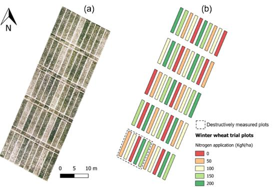
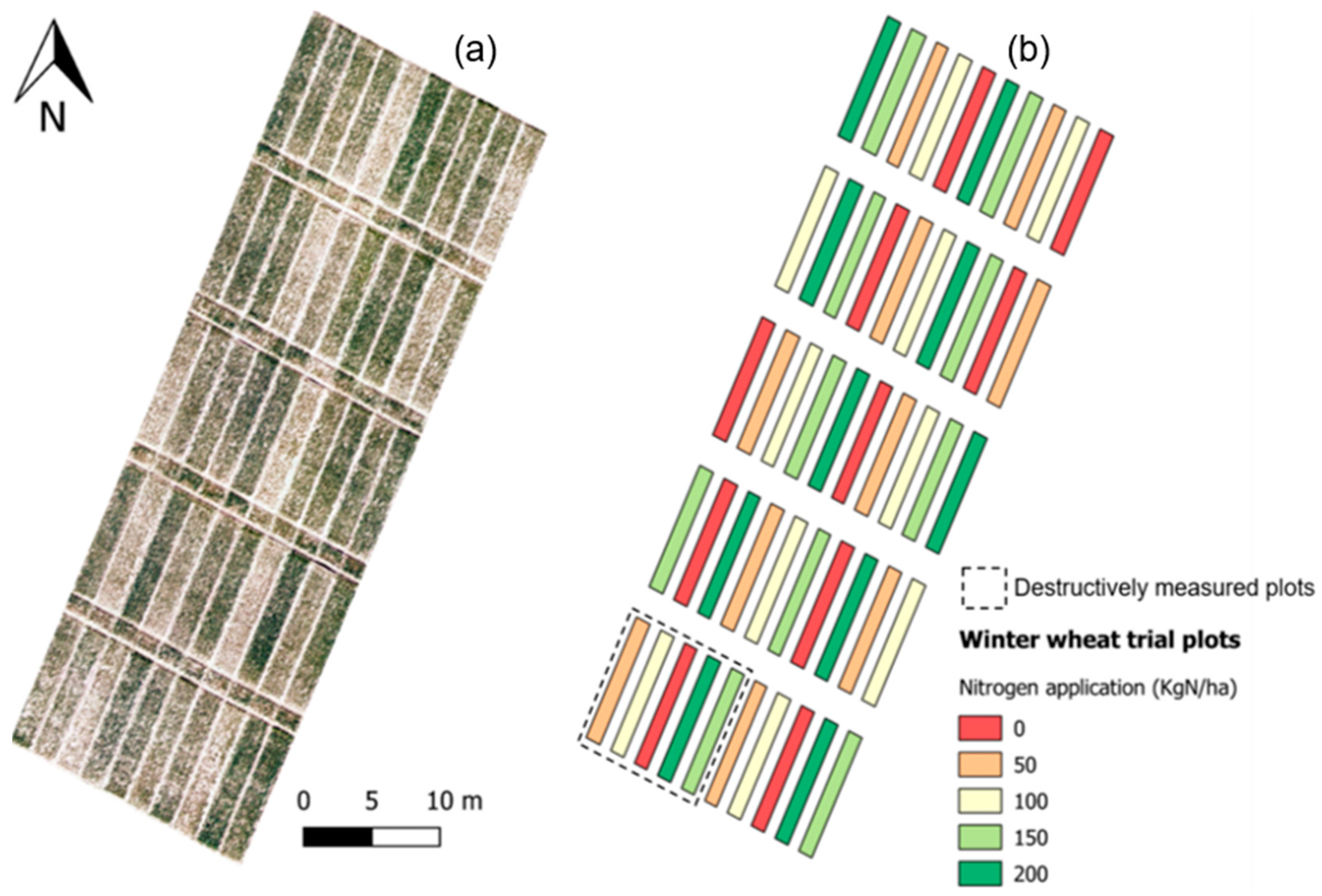
2.1.1. Experimental Trial Plot Description

The field experiment included a total of 50 winter wheat (Triticum aestivum L.) trial plots located approximately 3.8 km south of the village of East Saltoun, East Lothian, Scotland (55°52′50.5″ N, 2°50′12.2″ W; 170 m above sea level). The trial plots, with dimensions of 2 × 10 m, had a Latin square experimental design and, in order to induce variation in LAI, LCC and CCC, comprised five different levels of N application—0, 50, 100, 150 and 200 kg N ha⁻¹ (Figure 1) —each with five replicates for two common soft group 4 winter wheat varieties. These two wheat varieties—Revelation and Leeds—were included on the 2017/2018 recommended lists published by the U.K.’s Agriculture and Horticultural Development Board (AHDB) for cereals crops [34].

Each of the wheat plots were sown on 30 September 2017, in a roughly southwest to northeast direction with a seed rate of 340 seeds/m² and harvested on 25 August 2018. The soil was of the Humbie soil series with a loam texture. The N fertilisation of plots was carried out as a split application—50% of the total N was applied on 22 March 2018 and the remainder was added on 26 April 2018, which corresponded to growth stages (GS) 24 and 31, respectively. A herbicide based on the active ingredients picolinafen and pendimethalin was applied at GS11 on 27 October. A robust fungicide programme based on the active ingredients triazole, chlorothalonil, cyflufenamid, proquinazid, succinate dehydrogenase inhibitor and azoxystrobin, was also applied to all plots at four growth stages (GS30 on 16 April, GS32 on 9 May, GS39 on 30 May and GS65 on 22 June) to keep all diseases to a minimum level throughout the growing season.

2.1.2. In Situ Measurements

For five different dates within the growing season (

Table 1. Dates, corresponding average growth stages (GS; Zadoks scale) and weather conditions during ground and Unmanned Aerial Vehicle (UAV) multispectral measurement made at the winter wheat trial plots.

Ground and UAV Measurement Date (2018)	Growth Stage Description	Weather Conditions
08 May	Stem elongation—early (GS31)	Cloudy; low wind speed
25 May	Stem elongation—late (GS38)	Cloudy; low wind speed
05 June	Ear emergence (GS54)	Clear-sky; low wind speed
20 June	Flowering (GS68)	Clear-sky; moderate wind speed
04 July	Milk development (GS79)	Clear-sky; moderate wind speed

), non-destructive measurements carried out in each experimental trial plot included LAI, LCC and growth stage observations in accordance with the Zadoks decimal code [35]. Five technical replicates of LAI were taken per plot, with ten replicates of chlorophyll content on a regular grid within each plot. The replicates were then combined to give a plot average and standard deviation. The growth stage was assumed to be reached when it was observed in at least 50% of the plots. LAI was measured using a SunScan device (Delta-T Devices, Cambridge), and LCC measurements were inferred from a portable soil plant analyses development (SPAD) meter device (Konica Minolta, Japan). The CCC, expressed per unit of leaf area, was calculated as the product of the LAI and LCC [11,24,27]. Across the five observation dates and 50 trial plots, a total of 250 sets of LAI, LCC and CCC were derived from the ground measurements and were used in this study.

2.1.3. Destructive Sampling and Uncertainty Analysis

Destructive analyses were carried out to sample the winter wheat vegetation at five of the revelation trial plots, covering the range of N application from 0 to 200 kg (Figure 1). These destructive measurements, conducted on three dates (25 May, 13 June and 4 July 2018), were used to correct biases and quantify the uncertainty of LAI and LCC non-destructive measurements, which were also acquired on the same day as the destructive sampling. The measurements entailed randomly placing a 0.25 m² quadrat within the destructively-sampled plots and removing all above-ground vegetation. The leaves were separated from the remainder of the vegetation and the LAI was then estimated by passing the collected leaves through a Li-3100C leaf area meter (Li-Cor, Nebraska, USA). The non-destructive SunScan LAI estimates could then be directly compared to the destructive measurements to firstly correct for biases. This bias correction was performed through reduced major axis linear regression, which accounts for the variance in both the destructive and non-destructive measurements [36]. Specifically, the resultant linear fit equation was used to correct the bias in the non-destructive measurements. The uncertainty of the bias corrected non-destructive measurements was then calculated as the normalised root-mean-square-error (NRMSE):

$$NRMSE=\frac{\left[\sqrt{\frac{{{\displaystyle \sum }}_{i=1}^n{\left(E_i-O_i\right)}^2}{n}}\right]}{\left[\max \left(O\right)-\min \left(O\right)\right]},$$

(1)

where $E_i$ and $O_i$ represent the bias corrected non-destructive and destructive values, respectively, and $n$ is the number of non-destructive and destructive comparisons.

Past research has demonstrated a significant relationship between LCC and leaf N content [14]. We, therefore, quantified the uncertainty of the in situ LCC measurements by estimating the leaf N content of the destructive samples. This analysis involved drying and milling the samples for each vegetation material type (i.e. stem, leaves and ears). The samples were then weighed and analysed for percentage C and N content using a Flash 2000 elemental analyser. The SPAD LCC estimates were then compared to the average leaf N percentage for each of the five destructive sample plots.

2.2. UAV Platform and Data

2.2.1. UAV Platform and Multispectral Instrument

The UAV flights took place over the wheat trial plots on the corresponding ground measurement dates (Table 1) using a hexa-copter platform (DJI Matrice 600) at a height of 100 m above ground level and a constant speed of 3.1 m/s. Each of these flights were carried out close to solar noon (between 11:00 and 14:00 GMT+1) to avoid errors due to a low solar elevation angle. In order to ensure consistent and comparable multi-date coverage, the platform was equipped with a real-time kinematic Global Navigation Satellite System (GNSS) and was flown autonomously using the same flight mission, which was pre-programmed using the DJI Ground Station Pro software, for each of the measurement dates.

Multispectral imagery was acquired throughout the UAV flights using the MAIA camera system (SAL Engineering/EOPTIS), which is composed of an array of nine monochromatic sensors, each having a 1.2 Mpixel resolution. Furthermore, the nine sensors of the MAIA camera (referred to hereafter as the MAIA/Sentinel-2) have band-pass filters that have the same central wavelength and width as that of the first nine bands (i.e., bands 1 to 8A,

Table 2. Description of the MAIA/Sentinel-2 UAV multispectral camera bands and the corresponding Sentinel-2 multispectral instrument (MSI) bands, including the near-infrared (NIR) bands, and spatial resolution. Note: Band 1 (violet) was not used in the MAIA/Sentinel-2 band analysis.

MAIA/Sentinel-2				Sentinel-2 MSI
Band Number	Band Description	Central Wavelength (nm)	Band Width (nm)	Band Number	Spatial Resolution (m)
1	Violet	443	20	1	60
2	Blue	490	65	2	10
3	Green	560	50	3	10
4	Red	665	30	4	10
5	Red Edge1	705	15	5	20
6	Red Edge2	740	15	6	20
7	NIR 1	783	20	7	20
8	NIR 2	842	115	8	10
9	NIR 3	865	20	8A	20

) of the ESA Sentinel-2 multispectral instrument [37]. During the UAV flights, these sensors imaged the trial plots from a fixed nadir position with the aid of a three-axis stabilisation gimbal (DJI Ronin-MX).

The pixels in the nine MAIA/Sentinel-2 sensors collected data simultaneously via global shutters, thus allowing all the nine band images to be recorded in a single acquisition [38]. The sensors had horizontal and vertical angles of view of 33.4° and 25.5°, respectively, and a fixed focal length of 7.5 mm, which corresponded to a ground-sampling interval of 47 mm for our flight mission at 100 m above ground level. The MAIA/Sentinel-2 system also had a standard GNSS receiver that synchronously logged the position and time at which the camera’s shutter was activated. Throughout each of the UAV flights, a total of 18 MAIA/Sentinel-2 images were acquired over the trial plots and saved in a proprietary raw format with a 12-bit radiometric resolution.

2.2.2. Data Post-Processing

Image processing, including radial and radiometric calibration, was applied to the raw MAIA/Sentinel-2 imagery using the MultiCam Stitcher Pro software (v.1.1.8). The multiband images were first co-registered in order to correct the offsets between the nine sensors on the camera system. The radial calibration then involved a per-pixel correction for vignetting (i.e., the effect of a reduction in illumination from the centre to the edge of the image). To calculate ground-leaving reflectance, two identical white ground targets were placed at opposite ends of the UAV flight extents. Each target comprised a 1.0 m² panel that was made of a lambertian reflectant polyvinyl chloride (PVC)-coated material (‘Odyssey’ trademark material, Kayospruce Ltd.), which has previously been used in ESA remote sensing fieldwork campaigns [39]. At the beginning of each UAV flight, the spectral reflectance of these targets was measured using an Analytical Spectral Devices (ASD) FieldSpec Pro. This target reflectance was converted to absolute reflectance, following the guidelines outlined by the National Environment Research Council (NERC) Field Spectroscopy Facility [40]. These data were then convolved with the spectral response of each MAIA/Sentinel-2 band to correct the reflectance digital number (DN) recorded at pixels for each of the MAIA/Sentinel-2 spectral bands to absolute reflectance [37]:

$$D{N}_i^{\prime }=\frac{R{t}_i}{P{t}_i}\times D{N}_i,$$

(2)

where for each MAIA/Sentinel-2 band the corrected DN, $D{N}_i^{\prime }$, is calculated based on the ratio of the reference target spectra, $R{t}_i$, to the same value measured by the camera, $P{t}_i$.

We applied corrections to the recorded position of each of the MAIA/Sentinel-2 images by matching the GNSS time-stamp to that of the UAV platform. Consequently, with the time-stamps matched, we were able to use the more precise real-time kinematic GNSS position recorded in the UAV flight log. The collected images were then loaded into Agisoft PhotoScan Professional (v.1.3.3) where a photogrammetric workflow was applied to align and produce an othomosaic of the 18 multiband images covering the trail plots with a ground sampling resolution of 0.04 m.

The multiband MAIA/Sentinel-2 orthomosaics were overlaid with vector polygons for each of the 50 winter wheat trials plots. A buffer of −0.5 m was applied to the polygon edges in order to ensure a representative coverage of the trail plots. For each plot, the vector dataset was then used to extract mean pixel values recorded in the MAIA/Sentinel-2 dataset. Since band 1 of the MAIA/Sentinel-2 data is measured by the Sentinel-2 multispectral instrument at a 60 m spatial resolution (Table 2), we considered this resolution to be too coarse for precision agricultural applications and, therefore, we omitted this band and reduced the analysis to the eight remaining bands.

2.3. Band Analysis and Model Evaluation Approaches

The analysis of the eight MAIA/Sentinel-2 bands was carried out using the machine learning algorithm of Gaussian processes regression (GPR; [41]). Specifically, we applied GPR in order to determine the most informative MAIA/Sentinel-2 bands for the retrieval of LAI, LCC and CCC from the mean of the spectral data extracted at each trial plot. GPR provides a non-parametric and probabilistic modelling approach to establishing relationships between inputs (i.e. MAIA/Sentinel-2 bands) and outputs (vegetation variables), allowing for both the predictive mean and variance to be obtained [20,41,42]. Studies have demonstrated the calibration of GPR for the estimation of biophysical variables from satellite and airborne sensors [43,44] and has been shown to perform favourably in comparison to alternative machine learning algorithms [45].

Using the ARTMO (automated radiative transfer models operator) machine learning regression algorithms (MLRA) toolbox [46], we applied GPR as a scaled Gaussian kernel function (Equation (2); [20]):

$$k\left(x_i,x_j\right)=v\exp (-{{\displaystyle \sum }}_{b=1}^B\frac{{\left(x_i^b-x_j^b\right)}^2}{2{\mathsf{\sigma }}_b^2})+{\mathsf{\sigma }}_n^2{\delta }_{ij},$$

(3)

where for a given covariance function relating two observations, $k\left(x_i,x_j\right)$, the GPR model hyper parameters include the scaling factor,$v$, a standard deviation describing the variance of the estimates, ${\mathsf{\sigma }}_n$, and the length-scale, ${\mathsf{\sigma }}_b$, for each of the MAIA/Sentinel-2 bands, $b$. These hyper parameters, along with the model weight, are automatically optimised by maximising the marginal likelihood when training the GPR model using the MAIA/Sentinel-2 dataset and corresponding ground measurements for LAI, LCC and CCC. The inverse of ${\mathsf{\sigma }}_b$ represents the importance of each spectral band on $k$; accordingly, a higher ${\mathsf{\sigma }}_b^{-1}$ value indicates a higher information content when developing a GPR model for estimating a variable of interest.

To quantify the sensitivity of the MAIA/Sentinel-2 bands on the GPR model estimates, we trained the model using all 250 ground measurements recorded during the 2018 field campaign at the experimental trail plots and applied it within the ARTMO MLRA sequential backward band removal algorithm. This band removal algorithm entails an iterative procedure, whereby a GPR model is first developed using all eight MAIA/Sentinel-2 input bands. The least informative band (i.e., lowest ${\mathsf{\sigma }}_b^{-1}$) is then removed and a new GPR model is developed with the remaining bands, with this process repeating until the single most sensitive band remains. At each iteration of the backward band removal, we used the same input data for training and validating the GPR model. However, in order to ensure a robust analysis of each band, we applied a three-fold cross-validation sampling scheme. The GPR band analysis results, therefore, included the mean and standard deviation of the cross-validation statistics, including the coefficient of determination (R²) and the NRMSE.

From the statistical outputs of the sequential backward band removal procedure, we analysed the GPR models for each of the crop variables based on Akaike information criterion (AIC) [47]. AIC is an approach for model selection based on relative performance and works by balancing the trade-offs between model complexity (i.e., number of MAIA/Sentinel-2 bands) and goodness-of-fit against the validation data. We calculated the AIC based on the R² value for each GPR model [48]:

$$AI{C}_{gpr\_n}=-2\log \left[L\left(\widehat{\theta }\right)\right]+2K,$$

(4)

where the AIC of a GPR model, $AI{C}_{gpr\_n}$, is calculated based on the maximum likelihood of the parameter vector, $L\left(\widehat{\theta }\right)$, comprised of a number of bands, $K$. For each variable, the GPR model with the lowest AIC value was selected for further analysis. In order to determine the impact of uncertainty on GPR model development, this band analysis procedure was repeated both with and without the observational uncertainty. Our best performing GPR models for estimating LAI, LCC and CCC from the Sentinel-2 spectral data, with the propagated observational uncertainty, were further made available for the remote sensing community in a format that can be imported into the ARTMO MLRA toolbox (see the Supplementary Material).

In addition to the band analysis using the three-fold cross-validation statistics, we performed an independent validation of the GPR model performance by re-training the model with only half of the observations (i.e., with remaining observations used for validation). We further compared this independent model evaluation to a multivariate linear model, using ordinary least squares regression, which was developed using the most explanatory MAIA/Sentinel-2 bands and calibrated and validated using the same observations as the GPR model. We also quantified the spectral responses of these individual bands to the variables that were measured directly (i.e. LAI and LCC) and, in doing so, determined the extent to which these variables can be retrieved from the single bands. We thus compared the performance of the GPR approach to simple parametric models.

3. Results

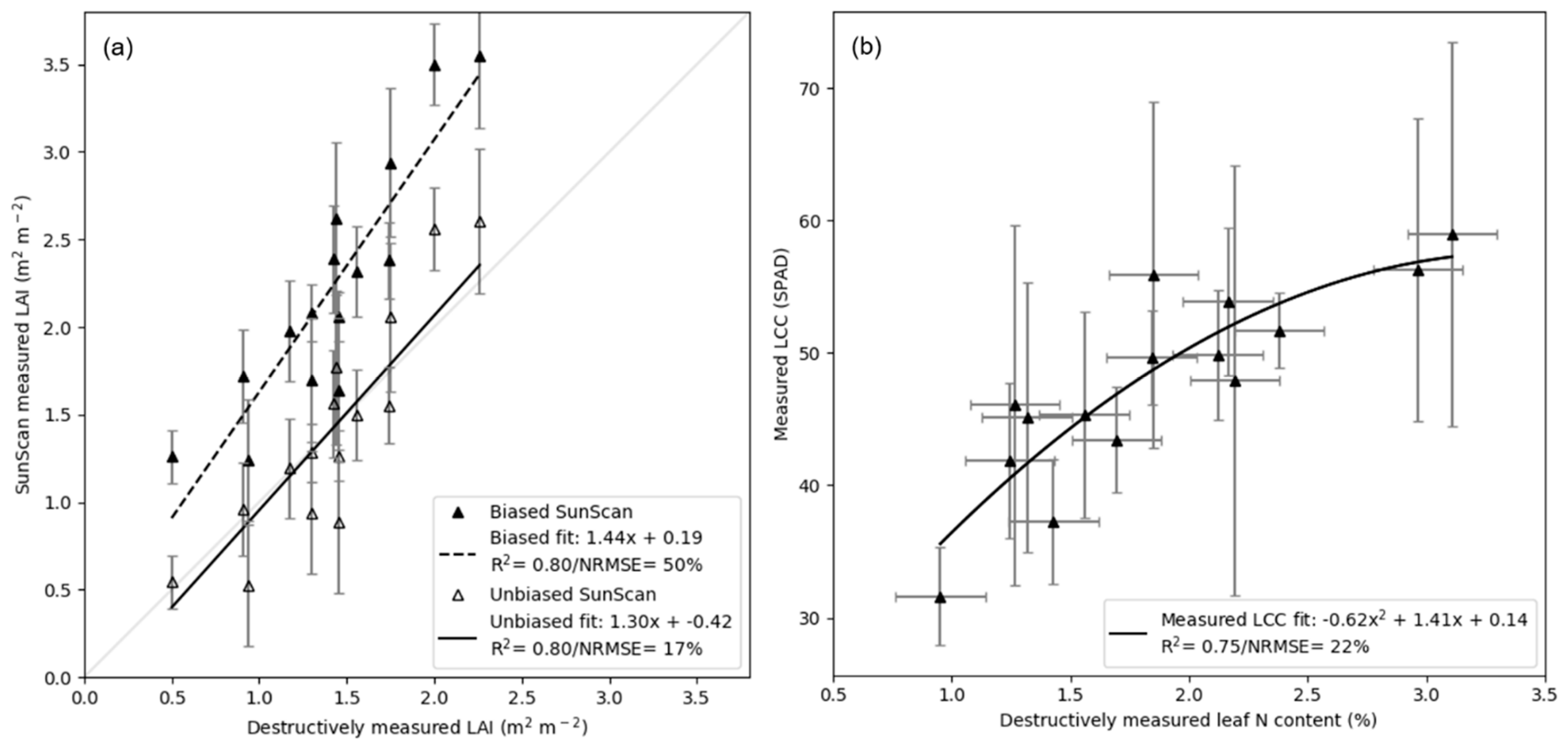
3.1. Uncertainty Analysis of In Situ Measurements

An overall high agreement existed between the in situ non-destructive measurements and destructive sample analysis (Figure 2). The R² was 0.80 for a linear fit between the SunScan and destructive sample LAI measurements. We further corrected the bias in the SunScan measurements based on the destructive data, which reduced the NRMSE from 50% to 17%. A quadratic fit demonstrated a high correlation (R² = 0.75) between the LCC measurements and leaf N content derived from the destructive sample analysis. The variance of the measured LCC was, however, relatively high when compared to that of the LAI, with the standard deviation of SPAD measurements ranging from +/- 3 to +/- 16.

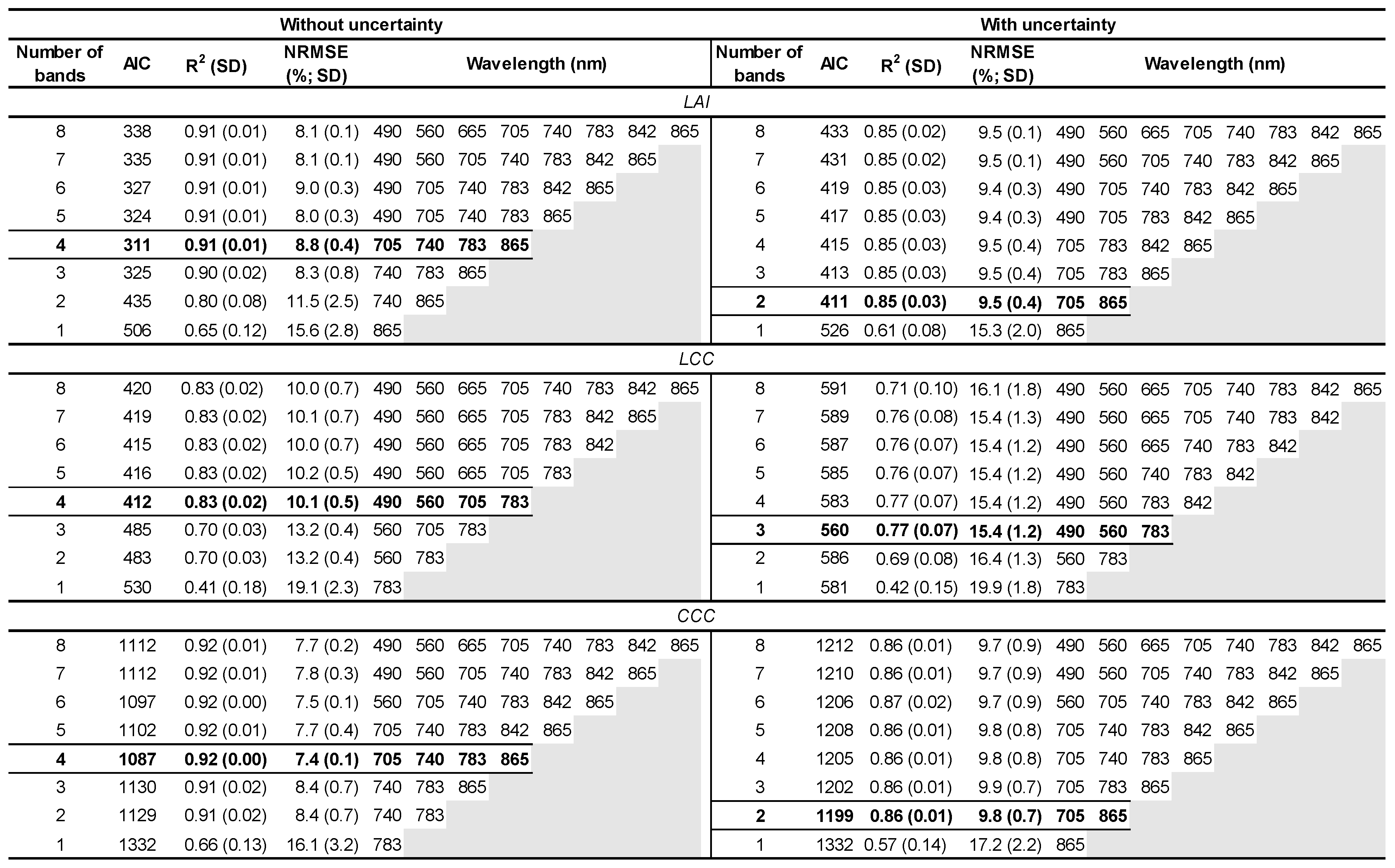
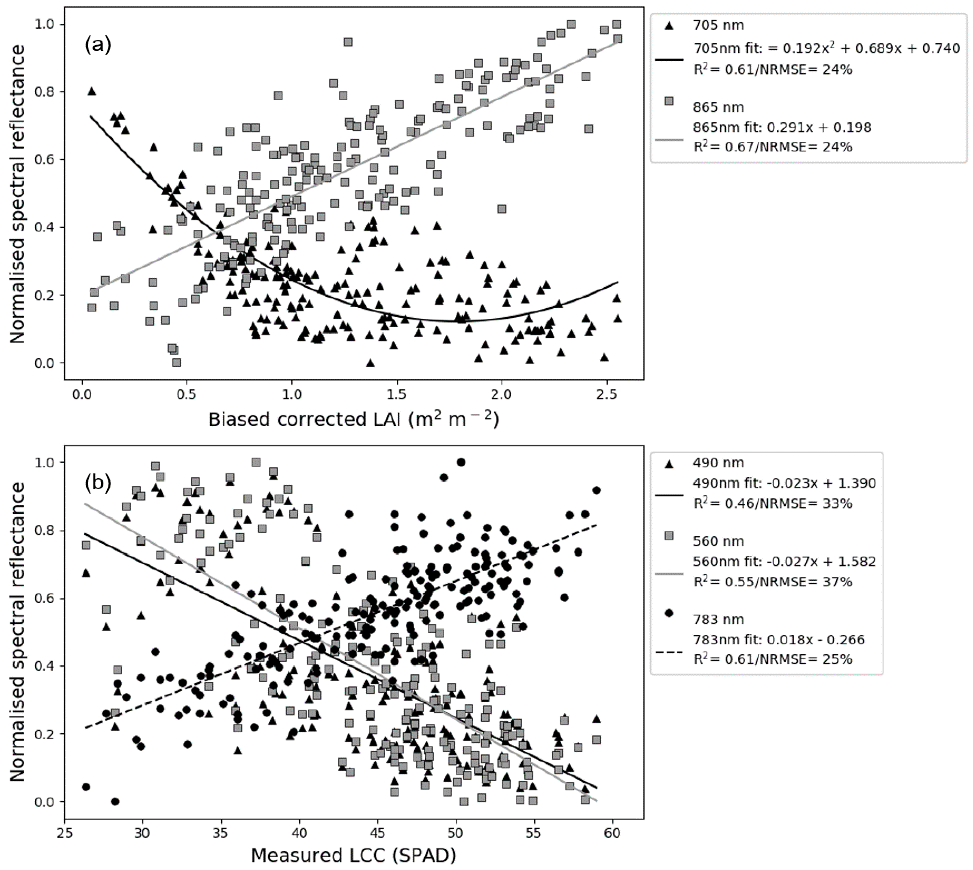
3.2. Sentinel-2 Band Analysis and Responses

Overall, the GPR model produced a high agreement with the LAI, LCC and CCC observations for all MAIA/Sentinel-2 band combinations (Figure 3). For the most explanatory band combinations, the mean R² was 0.89 and 0.83 without and with the propagated uncertainty, respectively. The model performance was greatest when estimating the CCC with the R² ranging from 0.92 (without uncertainty) to 0.86 (with uncertainty). On the basis of the standard deviations of R² and RMSE values, with the sequential band removal, the estimation uncertainty for each of the variables remained relatively stable until the successive removal of bands from the most explanatory band combinations, where error and uncertainty of these estimates sharply increased when using less than the optimum number of spectral bands.

In comparing the GPR band selection with and without propagating observational uncertainty, it was found that without uncertainty, the number of bands included in the optimum bands was four for each variable, whereas the number of key bands varied from two to three when including uncertainty (Figure 3). The MAIA/Sentinel-2 red-edge band at 705 nm and near-infrared 783 nm band were frequently included in the most explanatory band combinations. The selected band combinations for the estimation of LAI and CCC were identical—comprising two red-edge and two near-infrared bands (705, 740, 783 and 865 nm) for the GPR models without the observational uncertainty. For the models including uncertainty, however, the two most explanatory bands selected for estimating LAI and CCC were that of the red-edge (705 nm) and near-infrared 865 nm bands only.

For the most explanatory bands selected from the GPR framework developed with the propagated uncertainty, we analysed the sensitivity of these individual bands for estimating LAI and LCC based on the spectral responses to these two variables (Figure 4 and

Table 3. Summary of regression analysis statistics, including the coefficient of determination (R²) and normalised root-mean-square-error (NRMSE), from comparing single-band and multivariate linear regression and Gaussian processes regression (GPR) modelling for retrieving ground measurements of LAI and LCC.

	LAI		LCC
Modelling Approach	R2	NRMSE (%)	R2	NRMSE (%)
Individual bands	0.61 (705 nm)	24% (705 nm)	0.46 (490 nm)	33% (490 nm)
	0.67 (865 nm)	24% (865 nm)	0.55 (560 nm)	37% (560 nm)
			0.61 (783 nm)	25% (783 nm)
Multivariate linear regression	0.69	18%	0.67	13%
GPR	0.84	9%	0.60	18%

). The red-edge band at 705 nm showed a general exponential decrease in reflectance with increasing LAI (R² = 0.61), whereas the near-infrared band (865 nm) was characterised by a linear increase in reflectance with increasing LAI (R² = 0.67). For individual band responses to LCC, both the blue (490 nm) and green (560 nm) band reflectance exhibited a weak linear correlation (R² was 0.46 and 0.55 for the blue and green bands, respectively) with the reflectance in these bands decreasing with increasing LCC. Reflectance in the red-edge band (783 nm), however, showed a reasonable linear positive correlation (R² = 0.61) with increasing LCC.

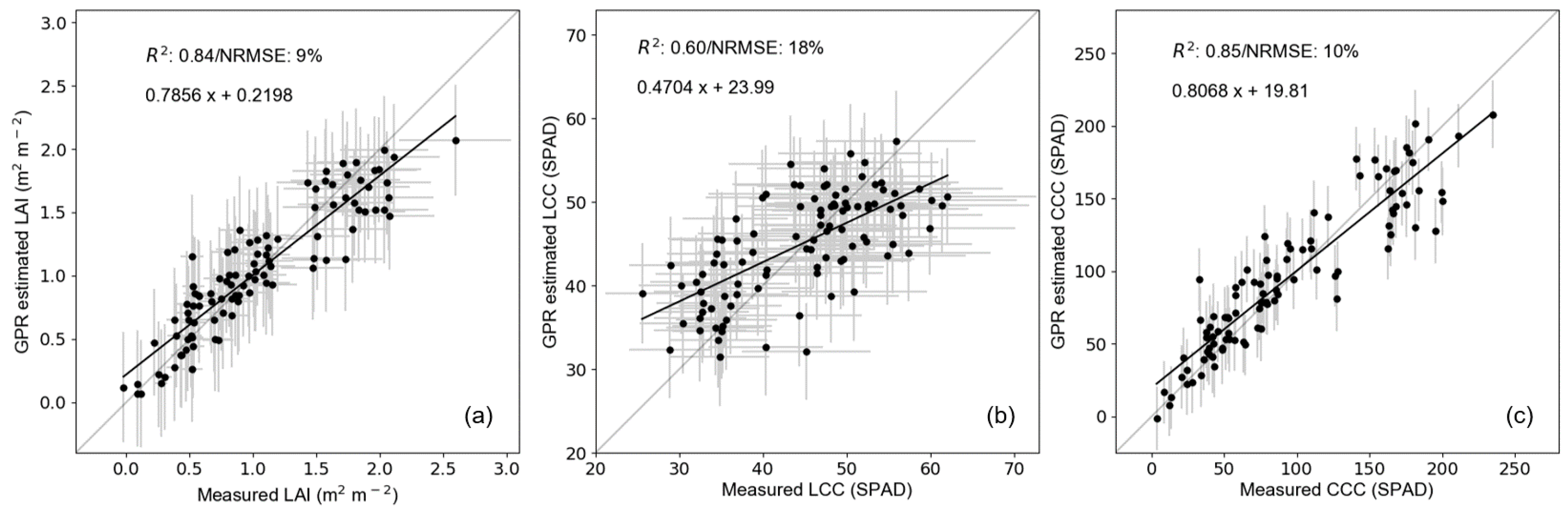
3.3. Independent Model Evaluation

The GPR model estimates when using the most explanatory band combinations demonstrated a high agreement to observations when validated using an independent dataset—the mean R² was 0.77 and the NRMSE was 12% (Figure 5 and Table 3). The GPR model performance was very similar when deriving the LAI and CCC estimates, with the R² being 0.85 for both variables and the NRMSE being 9 and 10% for LAI and CCC, respectively. In comparison to the other two variables, the model performance was weaker when estimating LCC, with R² and NRMSE being 0.60 and 18%, respectively.

When compared to the GPR model estimates, a multivariate linear regression model using the same dataset for calibration and validation showed a generally weaker performance in the estimation of all three variables, with the R² ranging from 0.67 to 0.73 (Figure 6). The LCC estimates by the linear regression model, however, had a higher agreement to the observations, with the R² and NRMSE being 0.67 and 13%, respectively.

4. Discussion

4.1. Ground Measurement Analysis and Uncertainty Characterisation

We quantified the uncertainty and bias of non-destructive measurements of LAI and LCC by comparisons to data derived from the destructive sub-sample analysis (Figure 2). The linear relationship established between the SunScan LAI and destructive measurements was biased (NRMSE = 62%), which was likely to have been due to the SunScan measurements over-estimating the LAI by including the contribution of stems and branches [49]. A non-linear relationship was observed between the LCC (SPAD) with increasing N content. This result is in agreement with research by Rostami et al. [50], where a quadratic plateau was observed between SPAD data with higher levels of N content in maize. In comparison to the LAI measurements, the LCC measurements made at each plot and sampling date were less consistent, which could be attributed to a high variability in the distribution of chlorophyll at both the leaf and canopy level [11,51].

4.2. Sentinel-2 Bands and GPR Modelling for Parameter Retrievals

Using UAV-based Sentinel-2 band observations and ground measurements, we assessed the capacity of the Sentinel-2 spectral bands for the retrieval of winter wheat LAI, LCC and CCC. We acknowledge that our GPR models for retrieving each of these variables were limited to one winter wheat season at our experimental field site. The calibration of the models was, however, carried out across multiple dates and N treatments; thus, covering a range of developmental stages and nutrient stresses. We would, therefore, expect the models to be broadly applicable when applied to retrieve the key variables from similar winter wheat varieties at alternative sites.

We exploited the band-ranking capabilities of a GPR machine learning algorithm and, in doing so, we objectively identified the most sensitive Sentinel-2 bands for retrieving each of these wheat variables. When we included the uncertainty of the ground measurements used in the training of the GPR models, it was found that two to three bands were sufficient for estimating the variables (Figure 3). Specifically, for the estimation of LAI and CCC without propagating the uncertainty, the optimum GPR model included both the red-edge bands (705 and 740 nm) and two of the near infra-red bands (783 and 865 nm). When propagating the uncertainty, the most informative bands included the red-edge band at 705 nm and near infra-red band at 865 nm only. This result suggests overfitting of the GPR model when variance in the training data is not accounted for and, thus, highlights the importance of propagating uncertainty in ground measurements when developing remote sensing retrieval algorithms. Being able to provide reliable estimates of the variables from a small number of well-defined Sentinel-2 bands also has the advantage of a reduction in processing time when generating high-resolution empirical retrieval maps of the variables over large areas [20]. More broadly, the ability to estimate multiple variables of a specific crop type using the essential spectral bands also has implications for the development of compact and lightweight UAV multispectral cameras [52].

Where the red-edge and near infra-red bands were favoured for the estimation of LAI and CCC, for the retrieval of LCC when the GPR model was developed with the propagated uncertainty, the optimum bands were composed of the visible blue (490 nm), green (560 nm) and near-infrared bands (783 nm). The sensitivity of the green and infrared bands for the estimation of LCC has previously been demonstrated [9,27]. Specifically, the Green Chlorophyll Vegetation Index (near infra-red/green; [31]) has successfully been applied in several studies for deriving crop chlorophyll content [24,53,54,55]. Research by Wang et al. [56] involved the analysis of winter wheat spectral reflectance under different N applications and demonstrated that bands centred around the green and near-infrared spectral regions were sensitive to the treatments, whereas the blue band was comparatively less sensitive. In our analysis, the inclusion of the blue band in the most informative band combination for LCC was, therefore, unexpected, but did appear to improve the performance of the GPR model when compared to using the green and near-infrared bands only. Our analysis also demonstrated a relationship between blue reflectance and LCC measurements (Figure 4).

The traditional approaches for retrieving biophysical parameters from Earth observation data have involved VIs, whereas our GPR machine learning approach allows a more thorough exploration of the sensitivity of each band to the measured variable without making assumptions. From applying the GPR model within the band analysis framework, the most informative Sentinel-2 bands that we identified were also situated around spectral regions of known reflectance and absorption and had a reasonable relationship to the ground measurements when evaluated individually (Figure 4). The sensitivity of these spectra to the biophysical variables is also broadly in agreement with past research [11,25,32,33]. We acknowledge, however, that our calibrated GPR modelling approaches are based on near-Earth (i.e., UAV) observations and, when applied to satellite-based observations, the retrieval accuracy would be subject to atmospheric effects. Research in Clevers et al. [24] has demonstrated a good agreement between atmospherically-corrected Sentinel-2 reflectance and ground-based radiometer measurements for potato crops. Nonetheless, we recommend additional testing of the robustness and a quantification of the uncertainty of the retrieval algorithms when applied to data acquired from the Sentinel-2 platform. Using an independent dataset for calibration and validation and the most informative bands, we also demonstrated that a simpler model approach of multivariate linear regression could provide generally comparable results to the GPR model (Figure 5 and Figure 6). Verrelst et al. [57] discusses the computation limitations of applying GPR models to large datasets and, therefore, the simpler regression approach may be more practical when retrieving pixel-level estimates of the variables across regional and country scales.

4.3. Potential of Sentinel-2 for Supporting Agricultural Management

The recent availability of open-access data from the Sentinel-2 dual-satellite constellation provides opportunities for the development and improvement of spatial data products that can support precision agriculture. Where past Earth observation satellite sensors (including SPOT-6/7 and Landsat-7/8) have relied on observations in the visible and near-infrared wavebands, this research has demonstrated that the two Sentinel-2 red-edge bands were frequently included within the most sensitive band combinations for retrieving key crop variables.

We have demonstrated the potential of the Sentinel-2 bands for providing more accurate estimates of LAI, which would be of value for improving the efficiency of crop model-data assimilation approaches, particularly when spatially upscaling model estimates from fields to regional extents [3,58]. In this research, we have shown a high correlation (R² = 0.86) between LCC and leaf N along with a high retrieval accuracy of LCC and CCC using Sentinel-2 bands. Being able to provide reliable estimates of LAI and chlorophyll content, i.e., as a proxy for N, is particularly useful for farmers when deciding on mid-season N fertilisation applications [18]. The traditional uniform approaches to fertiliser N applications are economically and environmentally inefficient, since they inherently ignore spatial heterogeneities in topography and soil properties [59,60]. The availability of timely and spatially explicit estimates of crop N content could be a crucial input for variable rate applications concerned with optimum N usage. Because of links between leaf N content and crop yields [50,61], within-field estimates of N could also be used to estimate crop yields. For use on an operational basis, the overall extent to which Sentinel-2 data can reliably support precision agricultural applications is, of course, dependent on the frequency of available cloud-free imagery. For our field site and growing season, we identified 19 cloud-free images. Since the period of time between successive observations ranged from 7 to 35 days, with an average of 17 days, this would not meet the biweekly observations recommended in previous research for tracking the temporal dynamics of crop growth [22,23]. However, these cloud-free images were within five days of each of the five growth stages targeted in this research and would be expected to be of value, particularly if the retrieved variables were used to update daily process-based crop models estimates.

The traditional approaches for variable retrieval use the visible red and near-infrared bands, which correspond to Sentinel-2 bands 4 and 8 that have a spatial resolution of 10 m (Table 2). On the other hand, the Sentinel-2 red-edge bands have a spatial resolution of 20 m. Although it is clear from this research that the red-edge bands improve estimates of LAI, LCC and CCC, for practical applications, the use of these bands would be at the expense of a reduction in spatial resolution. Löw and Duveiller [62] sampled from a continuum of increasingly coarser pixel sizes in order to investigate spatial resolution requirements for the image classification of different crop types. This research demonstrated that pixel sizes of around 117 m were sufficient to identify winter wheat, but this was found to be dependent on landscape heterogeneity (i.e., field size and shape) and timing within the growing season. Further research by Colombo et al. [63] showed stability in an LAI–VI relationship when spatially aggregating IKONOS satellite imagery pixels from 12 to 36 m. In our research we would, therefore, not anticipate any substantial increases in uncertainty when retrieving the crop variables at 20 m; the increase in performance when using the Sentinel-2 red-edge bands are likely to outweigh any negative impacts of a reduction in spatial resolution. Nonetheless, where our study focuses on the spectral characteristics of Sentinel-2, we would recommend future research related to Sentinel-2 spatial resolution that includes tracking the propagation of uncertainty when estimating variables using Sentinel-2 data at 10 and 20 m resolution for specific crop types.

5. Conclusions

This study has evaluated the Sentinel-2 satellite multispectral instrument spectral bands for the estimation of winter wheat variables—LAI, LCC and CCC—required for supporting precision agricultural technologies. Where past research has often used synthetic Sentinel-2 data within the growing season, here, we used data from a UAV-mounted multispectral camera with sensors matching the key Sentinel-2 wavebands. The acquisition of UAV multispectral data was carried out in coordination with ground measurements. These measurements, comprising destructive and non-destructive sample analysis data, were used to calibrate and validate the performance of a GPR machine-learning algorithm we applied to identify the most informative spectral bands for estimating each of the biophysical variables. The ground measurements were also used to quantify uncertainty that was propagated into the GPR model training data.

Overall, we have demonstrated a high retrieval accuracy of the variables when using the most informative Sentinel-2 bands (mean R² = 0.86). The Sentinel-2 red-edge and near-infrared bands were identified as being the most informative, particularly for LAI and CCC. The propagation of uncertainty in the ground measurement reduced the number of most informative bands, indicating an overfitting of the GPR model when uncertainty was not properly accounted for.

In comparison to previous satellite missions, the results we present highlight the potential of Sentinel-2 spectral data within an operational farm-scale decision support system. Future research should include testing the robustness and characterizing the uncertainty of the GPR modelling approach when applied to data acquired from the Sentinel-2 platform, including the uncertainty linked to the spatial scaling of these estimates to the resolution of Sentinel-2 multi-spectral instrument (i.e., 10 and 20 m). Furthermore, the use of GPR modelling, which provides a predictive mean and variance, would be an ideal approach for investigating the propagation of uncertainty from ground measurements to the scale of the Sentinel-2 sensor.

References

1. Zheng, G.; Moskal, L.M. Retrieving leaf area index (lai) using remote sensing: Theories, methods and sensors. Sensors (Basel Switz.) 2009, 9, 2719–2745. [Google Scholar] [CrossRef] [PubMed]
2. Aboelghar, M.; Arafat, S.; Saleh, A.; Naeem, S.; Shirbeny, M.; Belal, A. Retrieving leaf area index from spot4 satellite data. Egypt. J. Remote Sens. Space Sci. 2010, 13, 121–127. [Google Scholar] [CrossRef]
3. Huang, J.; Sedano, F.; Huang, Y.; Ma, H.; Li, X.; Liang, S.; Tian, L.; Zhang, X.; Fan, J.; Wu, W. Assimilating a synthetic kalman filter leaf area index series into the wofost model to improve regional winter wheat yield estimation. Agric. For. Meteorol. 2016, 216, 188–202. [Google Scholar] [CrossRef]
4. Li, H.; Chen, Z.; Liu, G.; Jiang, Z.; Huang, C. Improving winter wheat yield estimation from the ceres-wheat model to assimilate leaf area index with different assimilation methods and spatio-temporal scales. Remote Sens. 2017, 9, 190. [Google Scholar] [CrossRef]
5. Nearing, G.S.; Crow, W.T.; Thorp, K.R.; Moran, M.S.; Reichle, R.H.; Gupta, H.V. Assimilating remote sensing observations of leaf area index and soil moisture for wheat yield estimates: An observing system simulation experiment. Water Resour. Res. 2012, 48, W05525. [Google Scholar] [CrossRef]
6. Dorigo, W.A.; Zurita-Milla, R.; de Wit, A.J.W.; Brazile, J.; Singh, R.; Schaepman, M.E. A review on reflective remote sensing and data assimilation techniques for enhanced agroecosystem modeling. Int. J. Appl. Earth Obs. Geoinf. 2007, 9, 165–193. [Google Scholar] [CrossRef]
7. Sus, O.; Heuer, M.W.; Meyers, T.P.; Williams, M. A data assimilation framework for constraining upscaled cropland carbon flux seasonality and biometry with modis. Biogeosciences 2013, 10, 2451–2466. [Google Scholar] [CrossRef]
8. Revill, A.; Sus, O.; Barrett, B.; Williams, M. Carbon cycling of european croplands: A framework for the assimilation of optical and microwave earth observation data. Remote Sens. Environ. 2013, 137, 84–93. [Google Scholar] [CrossRef]
9. Gitelson, A.A.; Viña, A.; Verma, S.B.; Rundquist, D.C.; Arkebauer, T.J.; Keydan, G.; Leavitt, B.; Ciganda, V.; Burba, G.G.; Suyker, A.E. Relationship between gross primary production and chlorophyll content in crops: Implications for the synoptic monitoring of vegetation productivity. J. Geophys. Res. Atmos. 2006, 111. [Google Scholar] [CrossRef] [Green Version]
10. Osbourne, B.A.; Raven, J.A. Light absorption by plants and its implications for photosynthesis. Biol. Rev. 1986, 61, 1–60. [Google Scholar] [CrossRef]
11. Peng, Y.; Nguy-Robertson, A.; Arkebauer, T.; Gitelson, A.A. Assessment of canopy chlorophyll content retrieval in maize and soybean: Implications of hysteresis on the development of generic algorithms. Remote Sens. 2017, 9, 226. [Google Scholar] [CrossRef]
12. Takebe, M.; Yoneyama, T.; Inada, K.; Murakami, T. Spectral reflectance ratio of rice canopy for estimating crop nitrogen status. Plant Soil 1990, 122, 295–297. [Google Scholar] [CrossRef]
13. Yoder, B.J.; Pettigrew-Crosby, R.E. Predicting nitrogen and chlorophyll content and concentrations from reflectance spectra (400-2500 nm) at leaf and canopy scales. Remote Sensing Environ. 1995, 53, 199–211. [Google Scholar] [CrossRef]
14. Gholizadeh, A.; Saberioon, M.; Borůvka, L.; Wayayok, A.; Mohd Soom, M.A. Leaf chlorophyll and nitrogen dynamics and their relationship to lowland rice yield for site-specific paddy management. Inf. Process. Agric. 2017, 4, 259–268. [Google Scholar] [CrossRef]
15. Evans, J.R. Photosynthesis and nitrogen relationships in leaves of c3 plants. Oecologia 1989, 78, 9–19. [Google Scholar] [CrossRef] [PubMed]
16. Zhao, Y.; Chen, S.; Shen, S. Assimilating remote sensing information with crop model using ensemble kalman filter for improving lai monitoring and yield estimation. Ecol. Model. 2013, 270, 30–42. [Google Scholar] [CrossRef]
17. Rouse, J.W., Jr.; Haas, R.H.; Schell, J.A.; Deering, D.W. Monitoring vegetation systems in the great plains with ERTS. In Proceedings of the Third Earth Resources Technology Satellite-1 Symposium, Washington, DC, USA, 10–14 December 1974; pp. 301–317. [Google Scholar]
18. Cammarano, D.; Fitzgerald, G.; Casa, R.; Basso, B. Assessing the robustness of vegetation indices to estimate wheat n in mediterranean environments. Remote Sens. 2014, 6, 2827. [Google Scholar] [CrossRef]
19. Wang, L.; Chang, Q.; Yang, J.; Zhang, X.; Li, F. Estimation of paddy rice leaf area index using machine learning methods based on hyperspectral data from multi-year experiments. PLoS ONE 2018, 13, e0207624. [Google Scholar] [CrossRef]
20. Verrelst, J.; Rivera, J.P.; Gitelson, A.; Delegido, J.; Moreno, J.; Camps-Valls, G. Spectral band selection for vegetation properties retrieval using gaussian processes regression. Int. J. Appl. Earth Obs. Geoinf. 2016, 52, 554–567. [Google Scholar] [CrossRef]
21. Mulla, D.J. Twenty five years of remote sensing in precision agriculture: Key advances and remaining knowledge gaps. Biosyst. Eng. 2013, 114, 358–371. [Google Scholar] [CrossRef]
22. Becker-Reshef, I.; Vermote, E.; Lindeman, M.; Justice, C. A generalized regression-based model for forecasting winter wheat yields in kansas and ukraine using modis data. Remote Sens. Environ. 2010, 114, 1312–1323. [Google Scholar] [CrossRef]
23. Sakamoto, T.; Gitelson, A.A.; Arkebauer, T.J. Modis-based corn grain yield estimation model incorporating crop phenology information. Remote Sens. Environ. 2013, 131, 215–231. [Google Scholar] [CrossRef]
24. Clevers, J.; Kooistra, L.; van den Brande, M. Using sentinel-2 data for retrieving lai and leaf and canopy chlorophyll content of a potato crop. Remote Sens. 2017, 9, 405. [Google Scholar] [CrossRef]
25. Delloye, C.; Weiss, M.; Defourny, P. Retrieval of the canopy chlorophyll content from sentinel-2 spectral bands to estimate nitrogen uptake in intensive winter wheat cropping systems. Remote Sens. Environ. 2018, 216, 245–261. [Google Scholar] [CrossRef]
26. Horler, D.N.H.; Dockray, M.; Barber, J. The red edge of plant leaf reflectance. Int. J. Remote Sens. 1983, 4, 273–288. [Google Scholar] [CrossRef]
27. Gitelson, A.A.; Viña, A.; Ciganda, V.; Rundquist, D.C.; Arkebauer, T.J. Remote estimation of canopy chlorophyll content in crops. Geophys. Res. Lett. 2005, 32. [Google Scholar] [CrossRef] [Green Version]
28. Delegido, J.; Verrelst, J.; Meza, C.M.; Rivera, J.P.; Alonso, L.; Moreno, J. A red-edge spectral index for remote sensing estimation of green lai over agroecosystems. Eur. J. Agron. 2013, 46, 42–52. [Google Scholar] [CrossRef]
29. Clevers, J.G.P.W.; Kooistra, L. Using hyperspectral remote sensing data for retrieving canopy chlorophyll and nitrogen content. IEEE J. Sel. Top. Appl. Earth Obs. Remote Sens. 2012, 5, 574–583. [Google Scholar] [CrossRef]
30. Buschmann, C.; Nagel, E. In vivo spectroscopy and internal optics of leaves as basis for remote sensing of vegetation au buschmann, c. Int. J. Remote Sens. 1993, 14, 711–722. [Google Scholar] [CrossRef]
31. Gitelson, A.A.; Gritz, Y.; Merzlyak, M.N. Relationships between leaf chlorophyll content and spectral reflectance and algorithms for non-destructive chlorophyll assessment in higher plant leaves. J. Plant Physiol. 2003, 160, 271–282. [Google Scholar] [CrossRef]
32. Delegido, J.; Verrelst, J.; Alonso, L.; Moreno, J. Evaluation of sentinel-2 red-edge bands for empirical estimation of green lai and chlorophyll content. Sens. (Basel, Switz.) 2011, 11, 7063–7081. [Google Scholar] [CrossRef] [PubMed]
33. Clevers, J.G.P.W.; Gitelson, A.A. Remote estimation of crop and grass chlorophyll and nitrogen content using red-edge bands on sentinel-2 and-3. Int. J. Appl. Earth Obs. Geoinf. 2013, 23, 344–351. [Google Scholar] [CrossRef]
34. AHDB. Recommended Lists for Cereals and Oilseeds 2017/18; Agriculture and Horticulture Development Board: Warwickshire, UK, 2017. [Google Scholar]
35. Zadoks, J.C.; Chang, T.T.; Konzak, C.F. A decimal code for the growth stages of cereals. Weed Res. 1974, 14, 415–421. [Google Scholar] [CrossRef]
36. Isobe, T.; Feigelson, E.D.; Akritas, M.G.; Babu, G.J. Linear regression in astronomy. I. Astrophys. J. 1990, 364, 104–113. [Google Scholar] [CrossRef]
37. Nocerino, E.; Dubbini, M.; Menna, F.; Remondino, F.; Gattelli, M.; Covi, D. Geometric calibration and radiometric correction of the maia multispectral camera. Int. Arch. Photogramm. Remote Sens. Spat. Inf. Sci. 2017, XLII-3/W3, 149–156. [Google Scholar]
38. Dubbini, M.; Pezzuolo, A.; De Giglio, M.; Gattelli, M.; Curzio, L.; Covi, D.; Yezekyan, T.; Marinello, F. Last generation instrument for agriculture multispectral data collection. Agric. Eng. Int. CIGR J. 2017, 19, 87–93. [Google Scholar]
39. Vreys, K. Technical Assistance to Fieldwork in the Harth Forest During Sen2exp; Flemish Institute for Technological Research: Boeretang, Belgium, 2014; p. 105. [Google Scholar]
40. MacLellan, C. NERC Field Spectroscopy Facility-Guidlines for Post Processing ASD Fieldspec Proand Fieldspec 3 Spectral Data Files Using the FSF Ms Excel Template; National Centre for Earth Observation (NCEO): Edinburgh, Scotland, 2009; p. 18. [Google Scholar]
41. Rasmussen, C.E.; Williams, C.K.I. Gaussian Processes for Machine Learning; The MIT Press: New York, NY, USA, 2006. [Google Scholar]
42. Camps-Vails, G.; Gómez-Chova, L.; Muñoz-Mari, J.; Vila-Frances, J.; Amoros, J.; Valle-Tascon, S.D.; Calpe-Maravilla, J. Biophysical parameter estimation with adaptive gaussian processes. In Proceedings of the 2009 IEEE International Geoscience and Remote Sensing Symposium, Cape Town, South Africa, 12–17 July 2009; Volume 4, pp. IV-69–IV-72. [Google Scholar]
43. Verrelst, J.; Muñoz, J.; Alonso, L.; Delegido, J.; Rivera, J.P.; Camps-Valls, G.; Moreno, J. Machine learning regression algorithms for biophysical parameter retrieval: Opportunities for sentinel-2 and-3. Remote Sens. Environ. 2012, 118, 127–139. [Google Scholar] [CrossRef]
44. Lázaro-Gredilla, M.; Titsias, M.K.; Verrelst, J.; Camps-Valls, G. Retrieval of biophysical parameters with heteroscedastic gaussian processes. IEEE Geosci. Remote Sens. Lett. 2014, 11, 838–842. [Google Scholar] [CrossRef]
45. Verrelst, J.; Rivera, J.P.; Veroustraete, F.; Muñoz-Marí, J.; Clevers, J.G.P.W.; Camps-Valls, G.; Moreno, J. Experimental sentinel-2 lai estimation using parametric, non-parametric and physical retrieval methods – a comparison. ISPRS J. Photogramm. Remote Sens. 2015, 108, 260–272. [Google Scholar] [CrossRef]
46. Rivera, J.P.; Verrelst, J.; Muñoz-Marí, J.; Moreno, J.; Camps-Valls, G. Toward a semiautomatic machine learning retrieval of biophysical parameters. IEEE J. Sel. Top. Appl. Earth Obs. Remote Sens. 2014, 7, 1249–1259. [Google Scholar]
47. Akaike, H. A new look at the statistical model identification. IEEE Trans. Autom. Control 1974, 19, 716–723. [Google Scholar] [CrossRef]
48. Anderson, D.R.; Burnham, K.P.; White, G.C. Comparison of akaike information criterion and consistent akaike information criterion for model selection and statistical inference from capture-recapture studies. J. Appl. Stat. 1998, 25, 263–282. [Google Scholar] [CrossRef]
49. Bréda, N.J.J. Ground-based measurements of leaf area index: A review of methods, instruments and current controversies. J Exp. Bot. 2003, 54, 2403–2417. [Google Scholar] [CrossRef] [PubMed]
50. Rostami, M.; Koocheki, A.; Nassiri Mahallati, M.; Kafi, M. Evaluation of chlorophyll meter for prediction of nitrogen status of corn (zea mays). Am. Eurasian J. Agric. Environ. Sci. 2008, 3, 79–85. [Google Scholar]
51. Ciganda, V. Vertical profile and temporal variation of chlorophyll in maize canopy: Quantitative "crop vigor" indicator by means of reflectance-based techniques. Agron. J. 2008, 100, 1409–1417. [Google Scholar] [CrossRef]
52. Sankaran, S.; Khot, L.R.; Espinoza, C.Z.; Jarolmasjed, S.; Sathuvalli, V.R.; Vandemark, G.J.; Miklas, P.N.; Carter, A.H.; Pumphrey, M.O.; Knowles, N.R.; et al. Low-altitude, high-resolution aerial imaging systems for row and field crop phenotyping: A review. Eur. J. Agron. 2015, 70, 112–123. [Google Scholar] [CrossRef]
53. Dong, T.; Liu, J.; Shang, J.; Qian, B.; Ma, B.; Kovacs, J.M.; Walters, D.; Jiao, X.; Geng, X.; Shi, Y. Assessment of red-edge vegetation indices for crop leaf area index estimation. Remote Sens. Environ. 2019, 222, 133–143. [Google Scholar] [CrossRef]
54. Jay, S.; Baret, F.; Dutartre, D.; Malatesta, G.; Héno, S.; Comar, A.; Weiss, M.; Maupas, F. Exploiting the centimeter resolution of uav multispectral imagery to improve remote-sensing estimates of canopy structure and biochemistry in sugar beet crops. Remote Sens. Environ. 2018, 231, 110898. [Google Scholar] [CrossRef]
55. Magney, T.S.; Eitel, J.U.H.; Vierling, L.A. Mapping wheat nitrogen uptake from rapideye vegetation indices. Precis. Agric. 2017, 18, 429–451. [Google Scholar] [CrossRef]
56. Wang, C.; Feng, M.; Yang, W.; Ding, G.; Xiao, L.; Li, G.; Liu, T. Extraction of sensitive bands for monitoring the winter wheat (triticum aestivum) growth status and yields based on the spectral reflectance. PLoS ONE 2017, 12, e0167679. [Google Scholar] [CrossRef]
57. Verrelst, J.; Rivera, J.P.; Moreno, J.; Camps-Valls, G. Gaussian processes uncertainty estimates in experimental sentinel-2 lai and leaf chlorophyll content retrieval. ISPRS J. Photogramm. Remote Sens. 2013, 86, 157–167. [Google Scholar] [CrossRef]
58. Wu, S.; Huang, J.; Liu, X.; Fan, J.; Ma, G.; Zou, J.; Li, D.; Chen, Y. Assimilating Modis-Lai Into Crop Growth Model with Enkf to Predict Regional Crop Yield Computer and Computing Technologies in Agriculture V; Springer: Boston, MA, USA, 2012; Volume 370, pp. 410–418. [Google Scholar]
59. Basso, B.; Ritchie, J.T.; Cammarano, D.; Sartori, L. A strategic and tactical management approach to select optimal n fertilizer rates for wheat in a spatially variable field. Eur. J. Agron. 2011, 35, 215–222. [Google Scholar] [CrossRef]
60. Dumont, B.; Basso, B.; Bodson, B.; Destain, J.P.; Destain, M.F. Climatic risk assessment to improve nitrogen fertilisation recommendations: A strategic crop model-based approach. Eur. J. Agron. 2015, 65, 10–17. [Google Scholar] [CrossRef] [Green Version]
61. Cartelat, A.; Cerovic, Z.G.; Goulas, Y.; Meyer, S.; Lelarge, C.; Prioul, J.L.; Barbottin, A.; Jeuffroy, M.H.; Gate, P.; Agati, G.; et al. Optically assessed contents of leaf polyphenolics and chlorophyll as indicators of nitrogen deficiency in wheat (triticum aestivum l.). Field Crop. Res. 2005, 91, 35–49. [Google Scholar] [CrossRef]
62. Löw, F.; Duveiller, G. Defining the spatial resolution requirements for crop identification using optical remote sensing. Remote Sens. 2014, 6, 9034. [Google Scholar] [CrossRef]
63. Colombo, R.; Bellingeri, D.; Fasolini, D.; Marino, C.M. Retrieval of leaf area index in different vegetation types using high resolution satellite data. Remote Sens. Environ. 2003, 86, 120–131. [Google Scholar] [CrossRef]
Figure 1. Winter wheat trial plot layout including: (a) an aerial image (acquired on 15 May 2018) and (b) Latin square experimental design with varying levels of nitrogen application. Destructive sample analysis was carried out at five plots highlighted within the dashed line.
Remotesensing 11 02050 g001
Figure 2. Comparison of in situ non-destructive to mean destructive sample measurements acquired on three dates (25 May, 13 June and 4 July 2018) for five winter wheat trial plots, including (a) in situ measured Leaf Area Index (LAI) (SunScan) compared to LAI measured from destructive samples and (b) chlorophyll meter (soil plant analyses development (SPAD)) measured leaf chlorophyll content (LCC) compared to leaf nitrogen content measurements. Note: Fit line (black line) is defined using reduced major axis where y-axis error bars are derived from the standard deviations of non-destructive measurements and x-axis error bars represent the mean range between two destructive samples that were analysed for each plot.
Remotesensing 11 02050 g002
Figure 3. Sentinel-2 band analysis using Gaussian processes regression (GPR) modelling trained using multi-date wheat observation, both without (left) and with (right) accounting for uncertainty in observations, for deriving Leaf Area Index (LAI), leaf chlorophyll content (LCC) and canopy chlorophyll content (CCC). Statics include the mean and standard deviations of the coefficient of determination (R2) and normalised root-mean-square-error (NRMSE) from a three-fold cross-validation of the corresponding GPR models. The best performing GPR model, selected based on the lowest Akaike information criterion (AIC) value, is shown in boldface.
Remotesensing 11 02050 g003
Figure 4. Comparison of the normalised spectral responses and regression analysis between the most sensitive MAIA/Sentinel-2 bands and non-destructive ground measurements of (a) bias corrected LAI and (b) LCC.
Remotesensing 11 02050 g004
Figure 5. Independent GPR model evaluation for estimating (a) LAI, (b) LCC and (c) CCC. Note: Fit line (black line) is defined using reduced major axis where y-axis error bars are derived from the standard deviations of the GPR model estimates and x-axis error bars represent the standard deviations of the corresponding non-destructive ground measurements (available for LAI and LCC only).
Remotesensing 11 02050 g005
Figure 6. Independent evaluation of a multivariate linear regression model for (a) LAI, (b) LCC and (c) CCC.
Remotesensing 11 02050 g006