A Secchi Depth Algorithm Considering the Residual Error in Satellite Remote Sensing Reflectance Data

Abstract

1. Introduction
2. Methodology
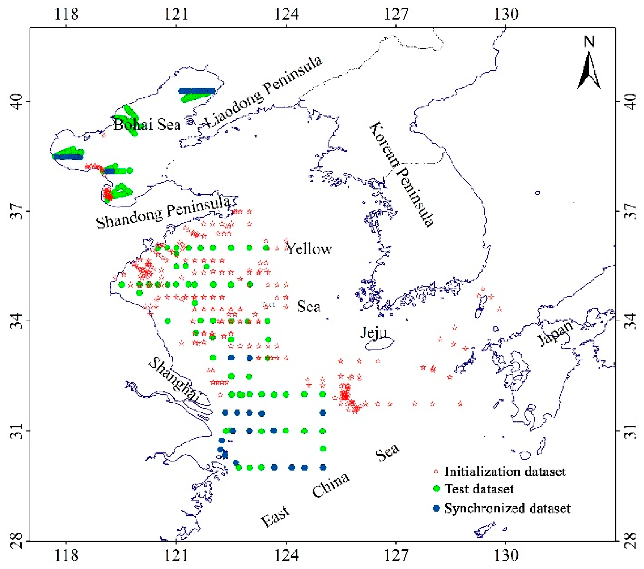
2.1. Study Area
2.2. In Situ Dataset
2.3. Synthetic Dataset
2.4. Satellite Image and Match-Up Data
2.5. The Overall Scheme for Derivation of Zsd and TSI
- (1)
- The IDAS model is utilized to calculate the a(λ) and bb(λ) from Rrs data. This model is a step-wise algorithm, with absorption and backscattering coefficients first derived at 555 nm, and then the estimations are extended to λ after applying a spectral model of the particle backscattering coefficient [21].
- (2)
- Lee et al. [18] showed that the Zsd is a function of Kd(λ), while Lee et al. [36] proposed that the Kd(λ) is a function of total absorption coefficient (a(λ)) and backscattering coefficient (bb(λ)). So Zsd should be a function of a(λ) and bb(λ). Thus, the relationship between Zsd and IDAS-derived a(λ) and bb(λ) are analyzed here. Based on the results of analyses, with a(488) and bb(488) as inputs, a new algorithm is developed for estimation of Zsd for both low and moderate turbid waters (denoted as Zsd,tc).
- (3)
- The optical properties are commonly very complicated in the extremely turbid waters [1], so it is not easy to derive a(λ) and bb(λ) from Rrs data with high quality in these waters. As a result, the semi-analytical algorithm in step 2 works well for low and moderate turbid waters but might be invalid for extremely turbid waters. Thus, an empirical approach is developed for predicting Zsd for extremely turbid waters (denoted as Zsd,et). This empirical algorithm denotes Zsd as a function of [Rrs(748) − Rrs(869)]−1, as the near-infrared wavelengths is more sensitive to changes of optically activity components than blue and green wavelengths in the extremely turbid waters. Following Hu et al. [28] and Chen et al. [21], band difference approach can absorb some residual error in satellite Rrs for Zsd retrieval, as the satellite residual error has good linear relationships between each other at the visible bands.
- (4)
- These two algorithms need to be combined to generate smooth Zsd data for low, moderate, and extremely turbid water, as well as waters of intermediate type. Thus, the linear weighting function (W) developed by Wang et al. [36] is applied for bridging two types of models for Zsd retrieval in the intermediate water type (denoted as Zsd,mt). Calibrated using initialization dataset, the optimal CSSD model can be found as follows (see Figure 2d):Here bbw is the backscattering coefficient of pure water; The parameter bbw(488)/bb(488) was used to minimize the effect of changing scattering agents [36,37].
2.6. Statistical Criterions for Product Evaluation
3. Results
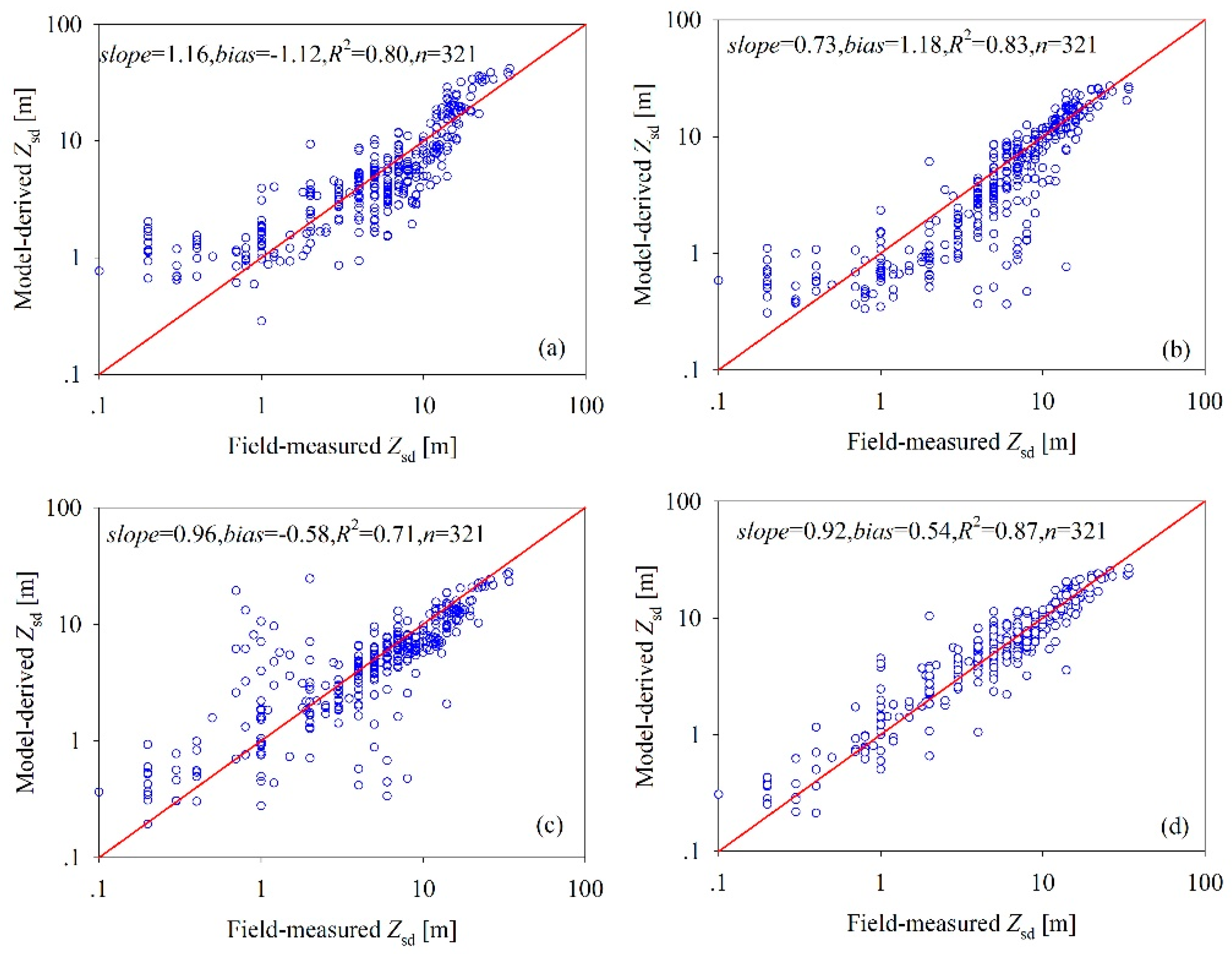
3.1. BGSD, IOPSD, MKSD, and CSSD Models Calibration
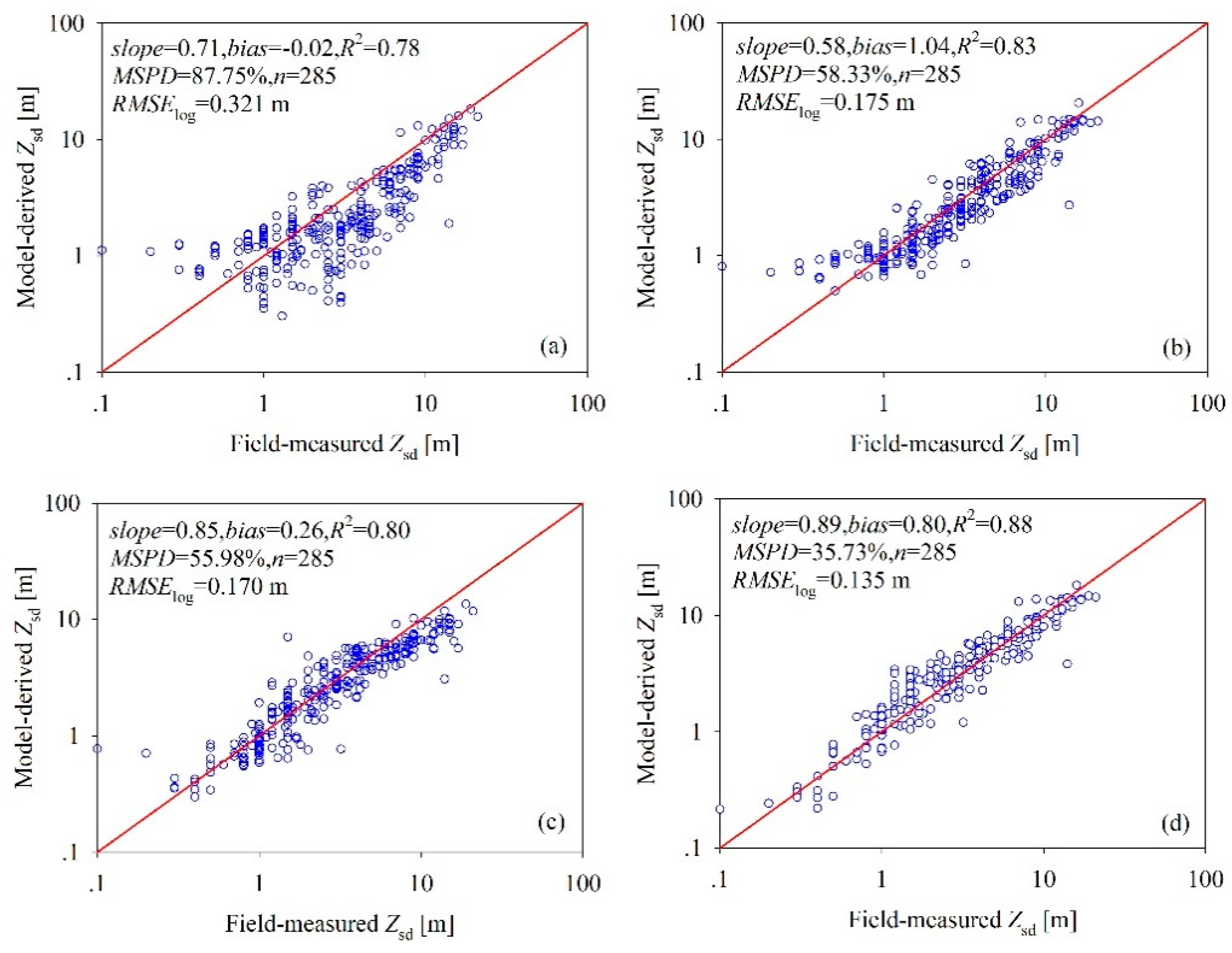
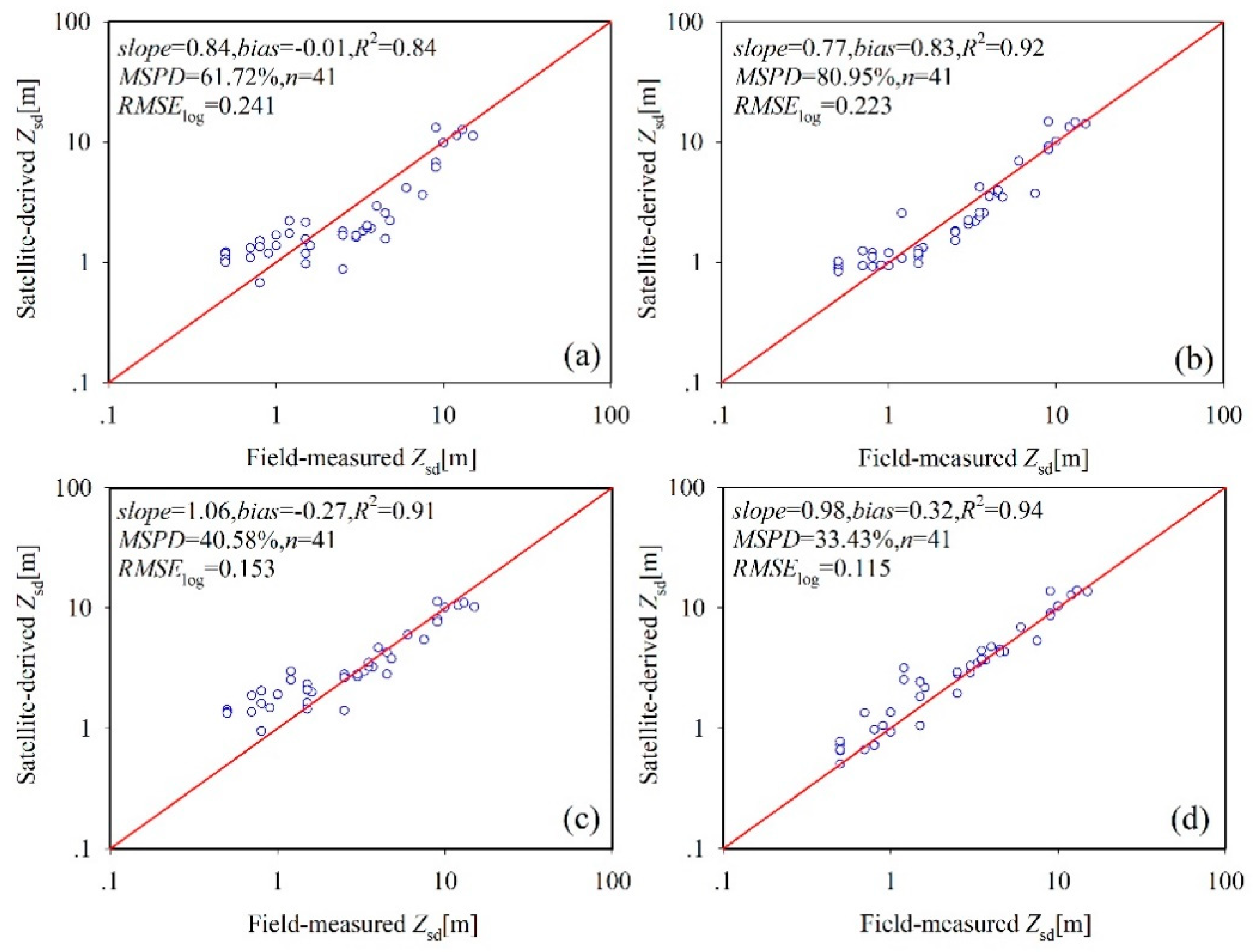
3.2. Model Evaluation and Comparisons
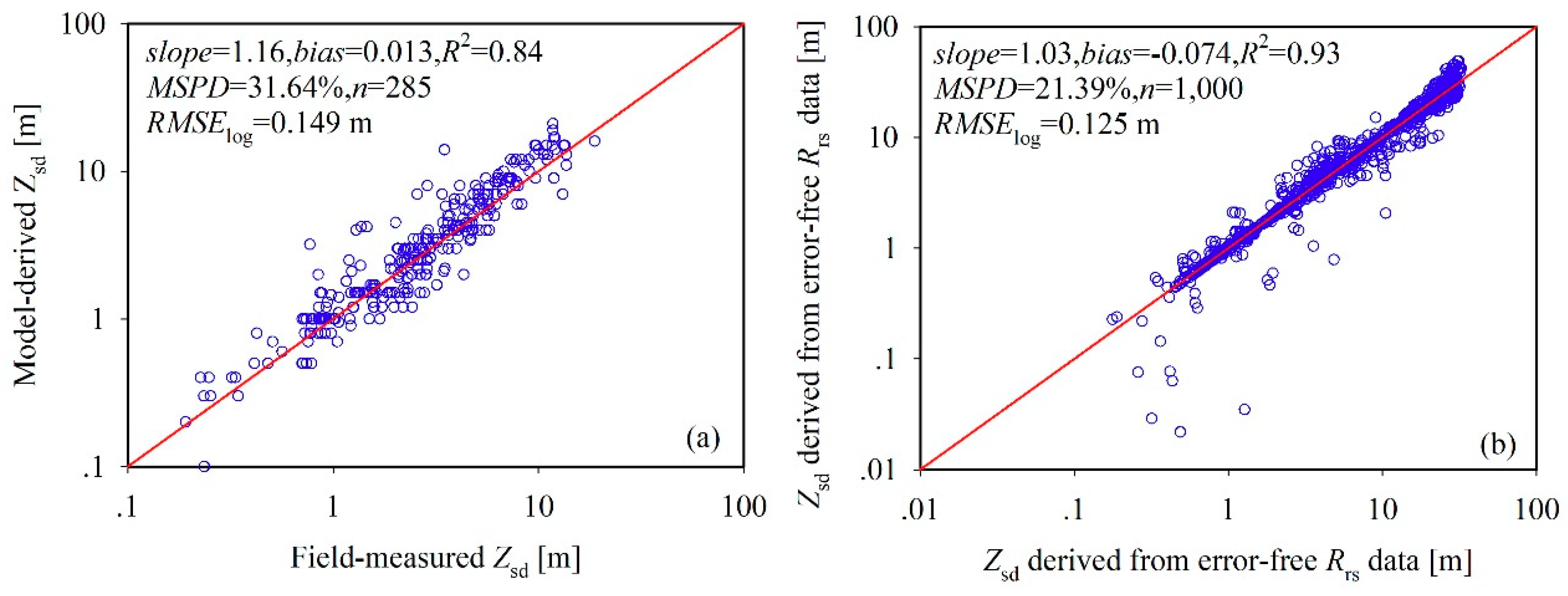
3.3. Match-Up Analysis
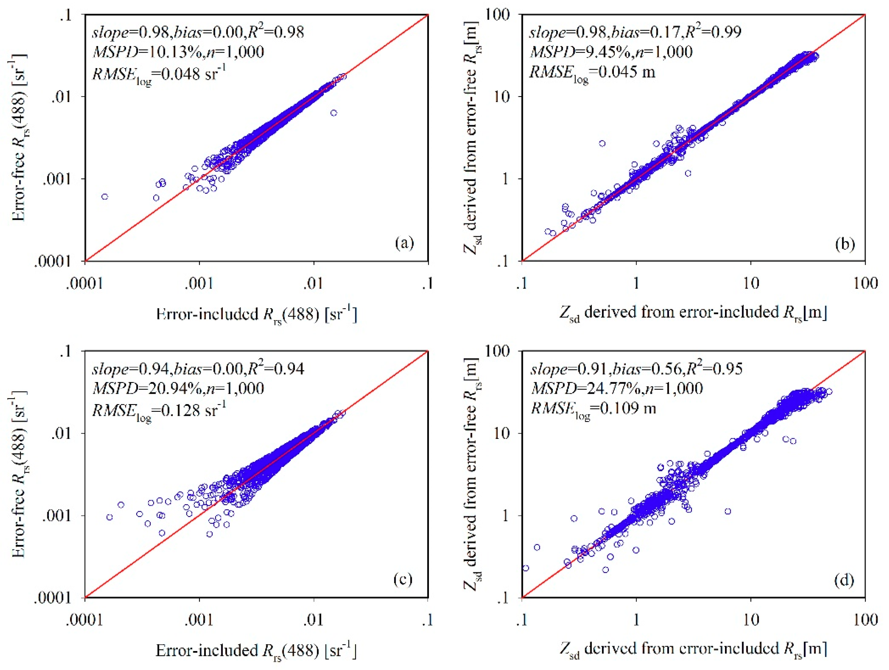
3.4. Noise Tolerance: IDAS-based Versus QAA-based CSSD Model
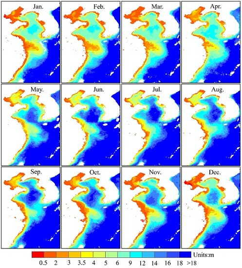
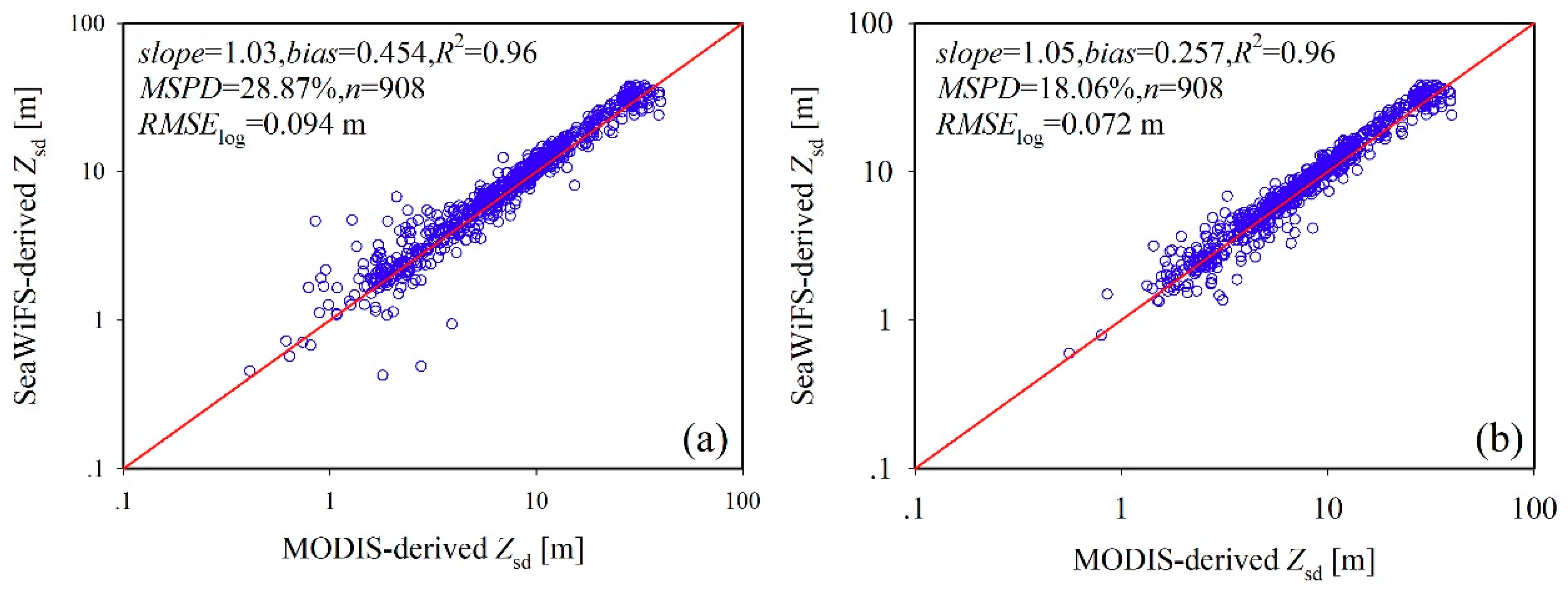
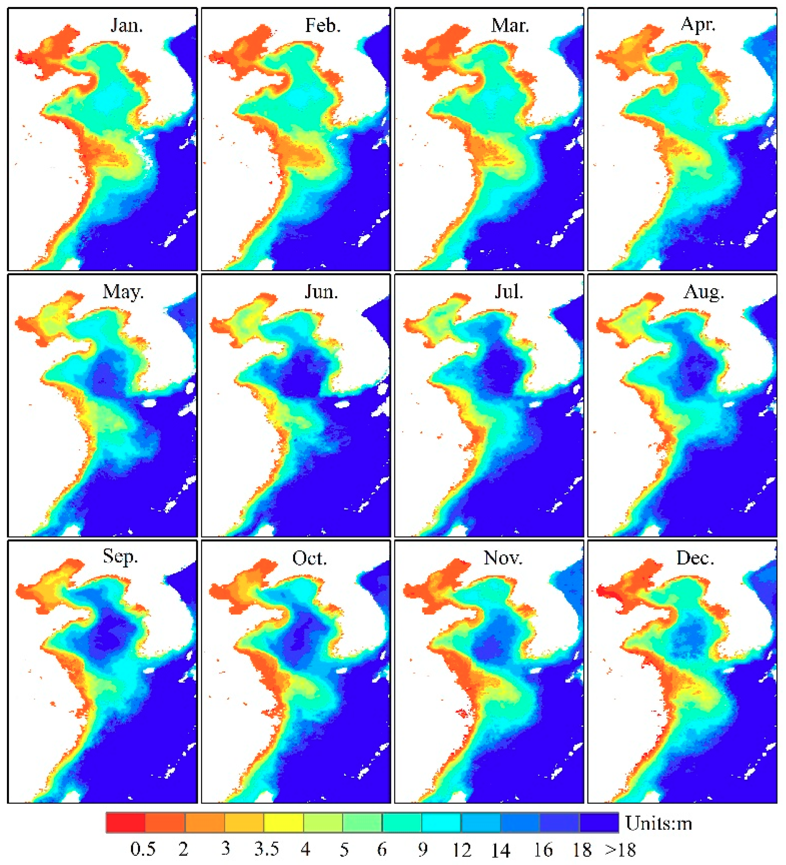
3.5. Spatial and Monthly Patterns of Secchi Depth
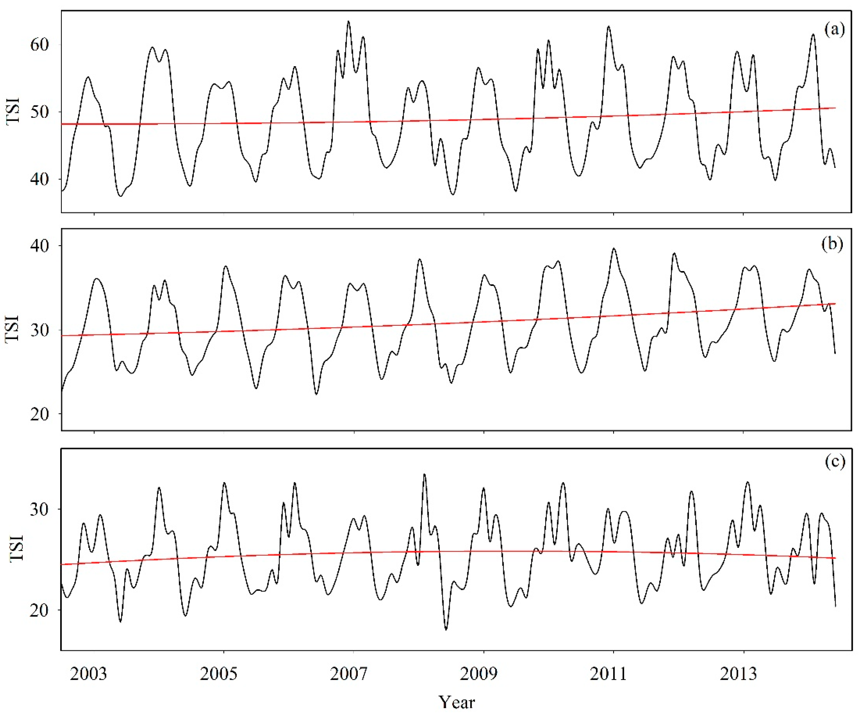
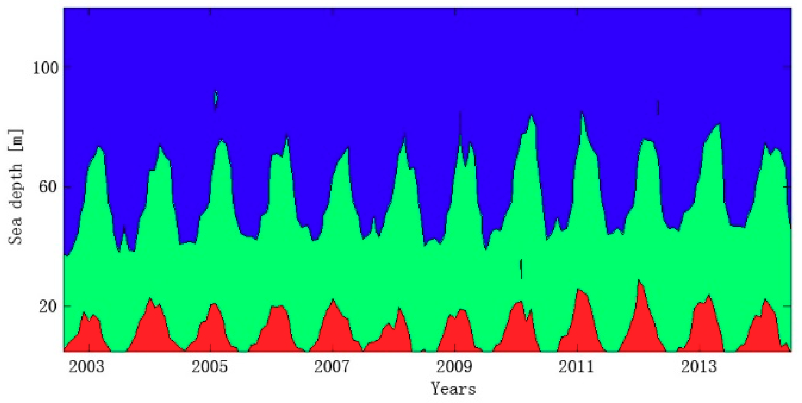
3.6. Spatial and Temporal Phases of Trophic State in the CECZ Seas
4. Discussion
5. Conclusion
Author Contributions
Funding
Acknowledgments
Conflicts of Interest
References
- Mobley, C.D. Light and Water: Tadiative Transfer in Natural Waters; Academic Press: Pittsburgh, PA, USA, 1994. [Google Scholar]
- Ibrahim, A.; Franz, B.; Ahmad, Z.; Healy, R.; Knobelspiesse, K.; Gao, B.C.; Proctor, C.; Zhai, P.-W. Atmospheric correction for hyperspectral ocean color retrieval with applications to the Hyperspectral Image for the Coastal Ocean (HICO). Remote. Sens. Environ. 2018, 204, 60–75. [Google Scholar] [CrossRef]
- Alikas, K.; Kratzer, S. Improved retrieval of Secchi depth for optically-complex waters using remote sensing data. Ecol. Indic. 2017, 77, 218–227. [Google Scholar] [CrossRef]
- Boyce, D.G.; Lewis, M.R.; Worm, B. Global phytoplankton decline over the past century. Nature 2010, 466, 591–596. [Google Scholar] [CrossRef] [PubMed]
- Onandia, G.; Gudimov, A.; Miracle, M.R.; Arhonditsis, G. Towards the development of a biogeochemical model for addressing the eutrophication problems in the shallow hypertrophic lagoon of Albufera de Valencia, Spain. Ecol. Inform. 2015, 26, 70–89. [Google Scholar] [CrossRef]
- Harrington, J.A.; Schiebe, F.R. Remote sensing of Lake Chicot, Arkansas: Monitoring suspended sediments, turbidity, and Secchi depth with Landsat MSS data. Remote. Sens. Environ. 1992, 29, 15–27. [Google Scholar] [CrossRef]
- Wang, F.; Umehara, A.; Nakai, S.; Nishijima, W. Distribution of region-specific background Secchi depth in Tokyo Bay and Ise Bay, Japan. Ecol. Indic. 2019, 98, 397–408. [Google Scholar] [CrossRef]
- McCullough, I.M.; Loftin, C.S.; Sader, S.A. Combining lake and watershed characteristics with Landsat TM data for remote estimation of regional lake clarity. Remote. Sens. Environ. 2012, 123, 109–115. [Google Scholar] [CrossRef]
- Kratzer, S.; Hakansson, B.; Sahlin, C. Assessing Secchi and photic zone depth in the Baltic Sea from satelltie data. Ambio 2003, 32, 577–585. [Google Scholar] [CrossRef] [PubMed]
- Giardino, C.; Pepe, M.; Brivio, P.A.; Ghezzi, P.; Zilioli, E. Detecting chlorophyll. Secchi disk depth and surface temperature in a sub-alpine lake using Landsat imagery. Sci. Total. Environ. 2001, 268, 19–29. [Google Scholar] [CrossRef]
- Morel, A.; Prieur, L. Analysis of variances in ocean color. Limnol. Oceanogr. 1977, 22, 709–722. [Google Scholar] [CrossRef]
- Devlin, M.J.; Barry, J.; Mills, D.K.; Gowen, R.J.; Foden, J.; Sivyer, D.; Tett, P. Relaitonships between suspended particulate material, light atteunation and Secchi depth in UK marine waters. Estuar. Coast. Shelf Sci. 2008, 79, 429–439. [Google Scholar] [CrossRef]
- Hakanson, L. The relationship between salinity, suspended particulate matter and water clarity in aquatic systems. Ecol. Res. 2006, 21, 75–90. [Google Scholar] [CrossRef]
- Fleming-Lehtinen, V.; Laamanen, M. Long-term changes in Secchi depth and the role of phytoplankton in explaining light attenuation in the Baltic Sea. Estuar. Coast. Shelf Sci. 2012, 102, 1–10. [Google Scholar] [CrossRef]
- Doron, M.; Babin, M.; Hembise, O.; Mangin, A.; Garnesson, P. Ocean transparency from space: validation of algorithms estimating Secchi depth using MERIS, MODIS and SeaWiFS. Remote. Sens. Environ. 2011, 115, 2986–3001. [Google Scholar] [CrossRef]
- Tyler, J.E. The Secchi disc. Limnol. Oceanogr. 1968, 13, 1–6. [Google Scholar] [CrossRef]
- Buiteveld, H. A model for calculation of diffuse light atteunation (PAR) and Secchi depth. Neth. J. Aquat. Ecol. 1995, 29, 55–56. [Google Scholar] [CrossRef]
- Lee, Z.; Shang, S.; Hu, C.; Du, K.; Weidemann, A.; Hou, W.; Lin, J.; Lin, G. Secchi disk depth: A new theory and mechanistic model for underwater visibility. Remote. Sens. Environ. 2015, 169, 139–149. [Google Scholar] [CrossRef]
- Jamet, C.; Loisel, H.; Dessailly, D. Retrieval of the spectral diffuse attenuation coefficient K-d(lambda) in open and coastal ocean waters using a neural network inversion. J. Geophys. Res. Oceans 2012. [Google Scholar] [CrossRef]
- Chen, J.; Ishizaka, J.; Zhu, L.Y.; Cui, T.W. A neural network model for Kd(λ) retrieval and application to global Kpar monitoring. PloS ONE 2015. [Google Scholar] [CrossRef]
- Chen, J.; Lee, Z.P.; Hu, C.M.; Wei, J.W. Improving satellite data products for open oceans with a scheme to correct the residual errors in remote sensing reflectance. J. Geophys. Res. Oceans 2016, 121, 3866–3886. [Google Scholar] [CrossRef]
- Hu, C.; Lee, Z.; Franz, B. Chlorophyll algorithms for oligotrophic oceans: A novel approach based on three-band reflectance difference. J. Geophys. Res. Oceans 2012. [Google Scholar] [CrossRef]
- Carlson, R.E. A trophic state index for lakes. Limnol. Oceanogr. 1977, 22, 361–369. [Google Scholar] [CrossRef]
- Liu, H.; Yin, B.S. Numerical investigation of nutrient limitations in the Bohai Sea. Mar. Environ. Res. 2010, 70, 308–317. [Google Scholar] [CrossRef] [PubMed]
- Wang, H.J.; Wang, A.M.; Bi, N.S.; Zeng, X.M.; Xiao, H.H. Seasonal distribution of suspended sediment in the Bohai Sea, China. Cont. Shelf Res. 2014, 90, 17–32. [Google Scholar] [CrossRef]
- Mueller, J.L.; Fargion, G.S.; McClain, C.R. Ocean Optics Protocols For Satellite Ocean Color Sensor Validation, Revision 4; Mueller, J.L., Fargion, G.S., McClain, C.R., Eds.; National Aeronautics and Space Administration publishing: Goddard Space Flight Center, WA, USA, 2003. [Google Scholar]
- IOCCG. Remote sensing of Inherent Optical Properties: Fundamentals, Tests of Algorithms, and Applications. Reports of the International Ocean Colour Coordinating Group No.5; IOCCG: Dartmouth, NH, Canada, 2006. [Google Scholar]
- Hu, C.M.; Feng, L.; Lee, Z.P. Uncertainties of SeaWiFS and MODIS remote sensing reflectance: implications from clear water measurements. Remote. Sens. Environ. 2013, 133, 168–182. [Google Scholar] [CrossRef]
- Gordon, H.R. Atmospheric correction of ocean color imagery in the earth observing system era. J. Geophys. Res. 1997, 102, 17081–17106. [Google Scholar] [CrossRef]
- Wang, M.; Shi, W. The NIR-SWIR combined atmospheric correction approach for MODIS ocean color data processing. Opt. Express 2007, 15, 15722–15733. [Google Scholar] [CrossRef] [PubMed]
- Wang, M.H.; Son, S.H.; Shi, W. Evaluation of MODIS SWIR and NIR-SWIR atmospheric correction algorithms using SeaBASS data. Remote Sens. Environ. 2009, 113, 635–644. [Google Scholar] [CrossRef]
- Huang, N.E. Computer implemented empirical mode decomposition method, apparatus, and article of manufacture for two-dimensional signals. US Patent US5983162, 1999. [Google Scholar]
- Werdell, P.J.; Bailey, S.W. The SeaWiFS bio-optical Archive and Storage System (SeaBASS): Current Architecture and Implementation. Goddard Space Flight Center, 2002. Available online: https://ntrs.nasa.gov/search.jsp?R=20020091607 (accessed on 31 December 2002).
- Bailey, S.W.; Werdell, P.J. A multi-sensor approach for the on-orbit validation of ocean color satellite data products. Remote Sens. Environ. 2006, 102, 12–23. [Google Scholar] [CrossRef]
- Lee, Z.P.; Werdell, P.J.; Arnone, R. An Update of the Quasi-analytical Algorithm (QAA_V5). IOCCG Software Report. 2009. Available online: www.ioccg.org/groups/Software OCA/QAAv5.pdf (accessed on July 2009).
- Lee, Z.P.; Hu, C.; Shang, S.; Du, K.; Lewis, M.; Arnone, R.; Brewin, R. Penetration of UV-Visible solar light in the global oceans: Insights from ocean color remote sensing. J. Geophys. Res. 2013, 118, 4241–4255. [Google Scholar] [CrossRef]
- Morel, A.; Antoine, D.A.; Gentili, B. Bidirectional reflectance of oceanic waters: accounting for Raman emission and varying particle scattering phase function. Appl. Opt. 2002, 41, 6289–6306. [Google Scholar] [CrossRef] [PubMed]
- Seegers, B.N.; Stumpf, R.P.; Schaeffer, B.A.; Loftin, K.A.; Werdell, J. Performance mertrics for the assessment of satellite data products: An ocean color case study. Opt. Express 2018, 19, 7404–7422. [Google Scholar] [CrossRef] [PubMed]
- Smyth, T.J.; Moore, G.F.; Hirata, T.; Aiken, J. Semi-analytical model for the derivation of ocean color inherent optical properties: Description, implementation, and performance assessment. Appl. Opt. 2006, 45, 8116–8132. [Google Scholar] [CrossRef] [PubMed]
- Garver, S.A.; Siegel, D.A. Inherent optical property inversion of ocean color spectral and its biogeochemical interpretation. 1. time series from the Sargasso Sea. J. Geophys. Res. Oceans 1997, 102, 18607–18625. [Google Scholar] [CrossRef]
- MacDonald, M.D.; Ruebens, M.; Wang, L.; Franz, B.A. The SeaDAS processing and analysis system: SeaWiFS, MODIS, and Beyond. In Proceedings of the American Geophysical Union, Fall Meeting, San Francisco, CA, USA, 5–9 December 2005. [Google Scholar]
- Wei, H.; Hainbucher, D.; Pohlmann, T.; Feng, S.; Suendermann, J. Tidal-induced Lagrangian and Eulerian mean circulation in the Bohai Sea. J. Mar. Syst. 2004, 44, 141–151. [Google Scholar] [CrossRef]
- Bi, N.; Yang, Z.; Wang, H.; Fan, D.; Sun, X.; Lei, K. Seasonal variation of suspended-sediment transport through the southern Bohai Strait. Estuar. Coast. Shelf Sci. 2011, 93, 239–247. [Google Scholar] [CrossRef]
- Wong, G.T.F.; Chao, S.Y.; Li, Y.H.; Shiah, F.-K. The Kuroshio edge exchange prcesses (KEEP) study-an introduction to hypotheses and highlights. Cont. Shelf Res. 2000, 20, 335–347. [Google Scholar] [CrossRef]
- Chang, P.H.; Isobe, A. A numerical study on the Changjiang diluted water in the Yellow and East China Seas. J. Geophys. Res. 2003. [CrossRef]
- Li, S.H.; Yun, C.X. Coastal current systems and the movement and expansion of suspended sediment from Changjiang River Estuary. Mar. Sci. Bull. 2006, 8, 22–33. [Google Scholar]
- Li, Y.; Li, A.; Huang, P.; Xu, F.; Zheng, X. Clay minerals in surface sediment of the north Yellow Sea and their implication to provenance and transportation. Cont. Shelf Res. 2014. [Google Scholar] [CrossRef]
- Yuan, J.; Hayden, L.; Dagg, M. Comment on “Reduction of primary production and changing of nutrient ratio in the East China Sea: Effect of the Three Gorges Dam” by Gwo-Ching Gong et al. Geophys. Res. Lett. 2007. [Google Scholar] [CrossRef]
- Liu, X.Y.; Liu, Y.G.; Guo, L.; Rong, Z.G.; Gu, Y.Z.; Liu, Y.Y. Interannual changes of sea level in the two regions of East China Sea and different responses to ENSO. Glob. Planet. Chang. 2010, 72, 215–226. [Google Scholar] [CrossRef]
- Spyrakos, E.; O’Donnell, R.; Hunter, P.D.; Miller, C.; Scott, M.; Simis, S.G.H.; Claudio, C.N.; Barbosa, C.F.; Binding, C.E.; Bradt, S.; et al. Optical types of inland and coastal waters. Limnol. Oceanogr. 2018, 63, 846–870. [Google Scholar] [CrossRef]
- Odermatt, D.; Gitelson, A.; Brando, V.E.; Schaepman, M. Review of constituent retrieval in optically deep and complex waters from satellite imagery. Remote. Sens. Environ. 2012, 118, 116–126. [Google Scholar] [CrossRef]


| Dataset | Variable | Min | Max | Median | Mean | Stdev |
|---|---|---|---|---|---|---|
| Initialization dataset (n = 321) | Rrs(667)/Rrs(488) | 0.004 | 1.689 | 0.342 | 0.425 | 0.372 |
| Zsd [m] | 0.100 | 34.00 | 6.000 | 7.376 | 6.155 | |
| Kd(488) | 0.032 | 4.406 | 0.308 | 0.684 | 0.894 | |
| Test dataset (n = 285) | Rrs(667)/Rrs(488) | 0.007 | 2.200 | 0.395 | 0.478 | 0.353 |
| Zsd [m] | 0.100 | 21.00 | 3.000 | 4.268 | 4.001 | |
| Kd(488) [m −1] | 0.084 | 4.374 | 0.418 | 0.739 | 0.807 | |
| Synchronized dataset (n = 285) | Rrs(667)/Rrs(488) | 0.063 | 1.128 | 0.401 | 0.510 | 0.319 |
| Zsd [m] | 0.500 | 15.00 | 2.500 | 3.686 | 3.742 | |
| Kd(488) [m −1] | 0.095 | 2.451 | 0.430 | 0.857 | 0.760 |
| TSI | Trophic State |
|---|---|
| TSI < 30 | Oligotrophic water |
| 30 ≤ TSI < 50 | Mesotrophic water |
| TSI ≥ 50 | Eutrophic water |
© 2019 by the authors. Licensee MDPI, Basel, Switzerland. This article is an open access article distributed under the terms and conditions of the Creative Commons Attribution (CC BY) license (http://creativecommons.org/licenses/by/4.0/).
Share and Cite
Chen, J.; Han, Q.; Chen, Y.; Li, Y. A Secchi Depth Algorithm Considering the Residual Error in Satellite Remote Sensing Reflectance Data. Remote Sens. 2019, 11, 1948. https://doi.org/10.3390/rs11161948
Chen J, Han Q, Chen Y, Li Y. A Secchi Depth Algorithm Considering the Residual Error in Satellite Remote Sensing Reflectance Data. Remote Sensing. 2019; 11(16):1948. https://doi.org/10.3390/rs11161948
Chicago/Turabian StyleChen, Jun, Qijin Han, Yanlong Chen, and Yongdong Li. 2019. "A Secchi Depth Algorithm Considering the Residual Error in Satellite Remote Sensing Reflectance Data" Remote Sensing 11, no. 16: 1948. https://doi.org/10.3390/rs11161948
APA StyleChen, J., Han, Q., Chen, Y., & Li, Y. (2019). A Secchi Depth Algorithm Considering the Residual Error in Satellite Remote Sensing Reflectance Data. Remote Sensing, 11(16), 1948. https://doi.org/10.3390/rs11161948