Estimating Forest Volume and Biomass and Their Changes Using Random Forests and Remotely Sensed Data

Abstract

Despite the popularity of random forests (RF) as a prediction algorithm, methods for constructing confidence intervals for population means using this technique are still only sparsely reported. For two regional study areas (Spain and Norway) RF was used to predict forest volume or aboveground biomass using remotely sensed auxiliary data obtained from multiple sensors. Additionally, the changes per unit area of these forest attributes were estimated using indirect and direct methods. Multiple inferential frameworks have attracted increased recent attention for estimating the variances required for confidence intervals. For this study, three different statistical frameworks, design-based expansion, model-assisted and model-based estimators, were used for estimating population parameters and their variances. Pairs and wild bootstrapping approaches at different levels were compared for estimating the variances of the model-based estimates of the population means, as well as for mapping the uncertainty of the change predictions. The RF models accurately represented the relationship between the response and remotely sensed predictor variables, resulting in increased precision for estimates of the population means relative to design-based expansion estimates. Standard errors based on pairs bootstrapping within or internal to RF were considerably larger than standard errors based on both pairs and wild external bootstrapping of the entire RF algorithm. Pairs and wild external bootstrapping produced similar standard errors, but wild bootstrapping better mimicked the original structure of the sample data and better preserved the ranges of the predictor variables.

1. Introduction

National forest inventories (NFIs) were initiated to collect information that could be used to ensure sustainable use of wood resources. As the forest functions of interest broadened, a substantial number of new variables were introduced to NFI field surveys [1] with growing forest stock volume and biomass now among the most commonly assessed. These variables are of fundamental importance for ensuring maintenance of wood production, formulating and implementing global forest policy, assessing sustainability, and improving decision-making regarding management decisions such as harvests. Traditionally, data obtained for ground plots that are spatially distributed using statistical sampling designs have satisfied the need for accurate forest parameter estimates, albeit at great cost and only for limited spatial and temporal scales. Remote sensing technologies provide valuable auxiliary information that can be used to enhance the precision and timeliness of forest parameter estimates [2,3,4].

On one hand, airborne laser scanning (ALS) has been claimed to be an outstanding information source for predicting vertical forest structure, with the result that numerous countries have allocated money to develop specific national programs for the purpose of acquiring ALS data [5]. The standard procedure for forest management inventory is the area-based approach (ABA). With ABA, models are used to describe relationships between field plot measurements and metrics derived from ALS point clouds with the models then applied to predict forest variables in a spatially continuous manner [6,7]. A great number of inventory attributes of interest have been predicted satisfactorily [6,8,9], even with low density ALS data [9,10,11]. Additionally, multi-temporal ALS data have been shown to be useful for modeling and predicting forest attribute changes [12,13,14]. These changes rely on two different methods: indirect and direct. The indirect method entails constructing a model for predicting the variable of interest for each point in time, whereas, the direct method predicts the change directly by creating change data as differences in the forest attribute between the two points [15,16]. On the other hand, forest attribute mapping methods have capitalized on the integration of ALS and multispectral data to achieve even more accurate and precise results [17,18].

The increased availability of free satellite imagery has also prompted development of additional inferential frameworks in which models are applied in large forest survey areas for the purpose of increasing the precision of forest attribute estimates [19,20,21]. For instance, model-assisted and model-based estimators have been applied successfully in large forest areas to estimate biomass [22,23] and volume [21,24] using mainly linear and nonlinear regression models. Model-assisted inference relies on a probability sampling (design-based) whereas model-based inference does not. Hence, the latter can be used with both non-probability sample data and data external to the area of interest [25,26]. This feature makes model-based inference a very interesting option for areas where design-based inference may be limited due to remoteness and inaccessibility [23]. However, the effectiveness of the model-based approach relies on the correctness of the model, and consequently model-based estimators may not be unbiased. Among the numerous modeling techniques, random forests (RF) has recently emerged as a popular one due to its ability to select and rank a large number of predictor variables [27] and its reliance on an ensemble of trees as a strategy to improve model robustness [14]. RF consists of a combination of decision trees where each tree contributes a single prediction for each population unit with the final prediction for each unit calculated as the mean over the RF tree predictions [28]. Each tree is independently constructed using a different randomly selected training sample obtained using bootstrap resampling procedures [27].

Although RF has been used extensively [16,29,30], little literature is available on model-based mean square error (MSE) estimation for population parameters with this algorithm. Bootstrap resampling methods have been used for model-based MSE estimation using multiple other prediction techniques [31,32,33]. These procedures are well-suited for applications requiring assumptions whose validity is difficult to assess and when only small sample sizes are available [34]. However, for RF models, general approaches for model-based MSE estimation merit additional attention [35] since estimates of MSE are necessary to construct inferences in the form of confidence intervals for population parameters.

The study objectives were threefold: (1) to construct RF models to predict response variables volume, biomass, and volume and biomass change for population units (ALS cells) in support of estimation of population and population change parameters such as mean volume per unit area and mean biomass per unit area; (2) to compare multiple bootstrap estimators of the model-based MSE of the estimate of the population mean; and (3) to construct change maps and change uncertainty maps. Two study areas were used, one in the La Rioja region of Spain and the other in Våler municipality, southeastern Norway (Figure 1). The Spanish data included plot-level volume datasets acquired at different times for different plots as well as corresponding ALS (2010–2016) and multi-spectral data. The Norwegian data included plot-level biomass datasets for two times for the same plots and temporally consistent ALS data (1999, 2010). Mean volume change per unit area was estimated with indirect methods for the Spanish study area and mean biomass change per unit area with direct methods for the Norwegian study area. Evaluation of the methods for two climatically different study areas, two response variables, and two approaches to estimating changes contributes to the robustness of the results and conclusions.

2. Materials and Methods

2.1. La Rioja, Spain

The study area is located in the La Rioja region of northern Spain (Figure 1) and consists of Scots pine (Pinus sylvestris L.) forests. According to the Spanish National Forest Inventory (SNFI), it is the second largest species formation in La Rioja, representing an area of approximately 27,000 hectares (ha), predominantly in zones above 1000 m elevation which cover the highest areas of the mountain regions. In general, La Rioja forests consist of pure and dense stands and were repopulated mainly due to the importance of their timber production. In addition, human depopulation of rural areas during recent decades has led to the natural expansion of the species. A Scots pine species mask was constructed based on the Spanish National Forest Map (SNFM25) (scale: 1:25,000). Forest land polygons of 1 ha minimum size in which Scots pine was the most dominant species were selected, resulting in a set of areas in which Scots pine was either monospecific or dominant but mixed with other species.

The data used to construct the RF volume models were obtained from two different surveys (

Table 1. Statistics for total volume (VOL) and aboveground biomass (AGB) obtained from the La Rioja sampling designs (La Rioja 2010 and La Rioja 2016) and the Våler sampling design.

Dataset	Variable	Number of Plots	Statistics
			Mean	Min	Max	Stdev
La Rioja 2010	VOL (m3/ha)	155	234.74	2.53	548.68	127.8
La Rioja 2016		49	236.53	5.21	517.15	135.39
Våler 1999	AGB (Mg/ha)	176	112.4	2.23	349.12	66.13
Våler 2010		176	131.15	0	462.17	91.83

): One characterized as La Rioja 2010 which consisted of ground data for a systematic sample of plots from the 4th SNFI and the first ALS acquisition (Section 2.1.1, first campaign), and the other characterized as La Rioja 2016 which consisted of ground data for a purposive sample of plots and the second ALS acquisition (Section 2.1.2, second campaign).

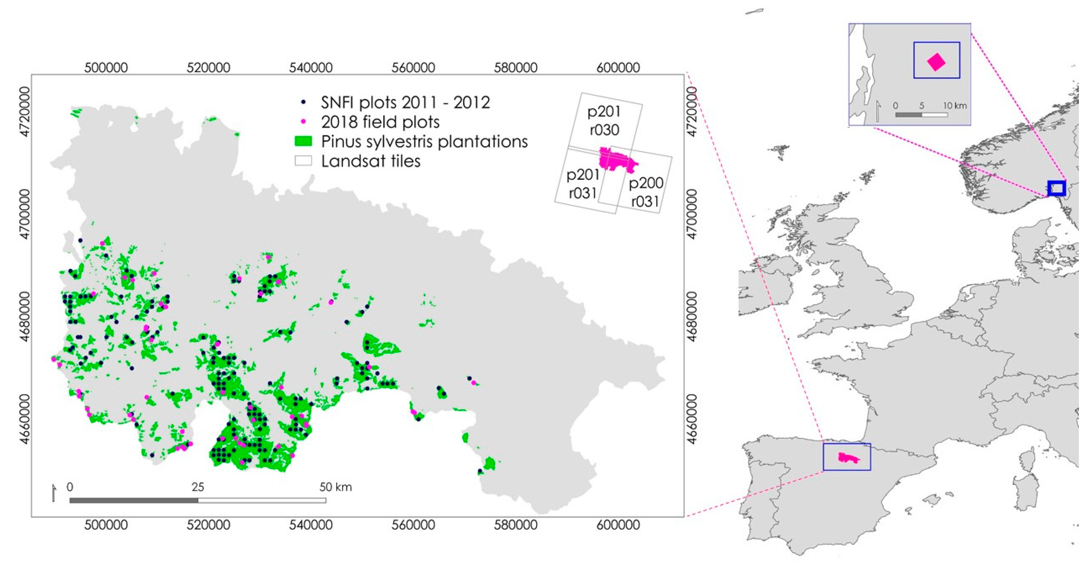
2.1.1. La Rioja Sampling Design

● First campaign

The 4th SNFI in La Rioja was conducted between 2011 and 2012 using permanent sample plots established systematically at the intersections of a 1 × 1 km grid in areas identified as forest land by the SNFM25 [36]. The SNFI sample units consist of four circular concentric plots of radius 5, 10, 15, and 25 m. Trees with diameter at breast height (DBH) of at least 75 mm are measured in a 5 m radius plot; trees with DBH >125 mm are measured in a 10 m radius plot; trees with DBH >225 mm are measured in a 15 m radius plot; and only trees with a DBH >425 mm are measured in the 25 m radius plot [36,37]. For each tree, DBH, total height, species, and the tree’s position relative to the plot center (direction and distance) are recorded. Species-specific allometric models were used to predict individual tree volumes which were weighted to predict the total plot stock volume [31]. We ignored the uncertainty associated with individual tree allometric volume predictions based on the findings of McRoberts et al. [38,39]. When the allometric models are based on large calibration datasets and when the model fits the data well, the effects of this model prediction uncertainty are small relative to the effects of plot-to-plot sampling variability. However, if smaller calibration samples sizes are used as in La Rioja 2016, the final uncertainty value could be underestimated.

All SNFI plots in the study area were filtered by selecting those for which the forest class under consideration was dominant (more than 80% of total volume). Furthermore, only plots whose maximum height (the height of the tallest tree, hmax) were consistent with the 99th height percentile, derived from ALS 2010, were considered due to inaccuracy of plot center coordinates (5–15 m [40,41]). This inaccuracy could lead to discrepancies between the field measured attribute and the population unit remote sensing metrics. SNFI plots were removed from the analysis when their respective hmax was different in the range of plus/minus 4 m with respect to the 99th height percentile. The resulting sample after filtering by both criteria consisted of 155 field plots.

● Second campaign

Field data for the second survey were acquired during the summer of 2018 for 49 circular plots with a 14.1 m radius. The center of each plot was recorded using a dual-frequency global navigation satellite system receiver GEO7x (Trimble^®GNSS) with sub-meter horizontal accuracy (0.4 m) after post-processing correction. DBH and species were recorded for all trees with DBH >75 mm. Height was measured for six randomly selected trees per plot. The heights of the remaining trees for each plot were predicted using a generalized height–diameter model based on the tree heights measured on all field plots. The total plot stock volume was predicted using the allometric models constructed by Crecente-Campo et al. [42] for Scots pine using 2682 plots located in the major mountain ranges of Spain.

The 49 circular plots were purposively selected considering the variability of the forest stands and their distribution over the study area. The aim was to achieve a specific distribution that encompasses different ranges and variability of forest structural attributes including height, forest canopy cover, canopy relief ratio, elevation, and slope. Additionally, these plots were selected based on their accessibility for field work, favoring those areas closest to forest tracks.

2.1.2. Remotely Sensed Data

ALS data were acquired in 2010 and 2016 during leaf-on conditions by the Spanish National Programme of Aerial Orthophotography with a mean density of 0.5 points per m² and vertical RMSE <0.4 m for the former and 2 points per m² and vertical RMSE <0.2 m for the latter. ALS tiles were processed using FUSION software [43] to generate a 2-m digital elevation model from the ground points, which facilitates estimation of height above the ground surface for each vegetation point. Fifteen forest structure metrics were calculated, having previously removed the points below 2 m, both for the field plots and 25-m × 25-m cells that tessellated the study area and served as population units. ALS metrics included mean, variance (varia), standard deviation (stdev), coefficient of variation (cv), interquartile range (iq), kurtosis (kurto), percentiles (ranging from the 1st to 99th percentile: p1, p5, p25, p50, p75, p95, and p99), canopy relief ratio (crr), and forest canopy cover (lfcc). The locations of the 25-m × 25-m cells were exactly the same for both ALS datasets. The 625 m² (25-m × 25-m) size for the population units was chosen because it is similar to the smallest sample plots (14.1 m radius; 625 m²) used for the second campaign. Even the smallest plots and the ALS cells had enough ALS points to estimate ALS metrics reliably. With a cell size of 625 m² and a minimum point density of 0.5 points per m², there would be, on average, 312.5 points per plot and cell. Based on Vauhkonen et al. [44], more than 300 points per plot should be sufficient.

The study area is covered by three Landsat scenes with paths (p) and rows (r): p201 r031, p200 r031, and p200 r030 (Figure 1). For each scene, two predominantly cloud free images (less than 10% cloud cover) were downloaded corresponding to the years for the two ALS datasets (2010 and 2016). From 18 July for p200 r030 and 23 June for the rest of Landsat scenes. Surface reflectance of individual bands (blue, green, red, near infrared (NIR), and two shortwave infrared (SWIR)) and their respective quality assurance (QA) bands were calculated. QA bands were used to remove the remaining cloud and cloud shadows.

Each image was resampled using the nearest neighbor resampling method from 30-m × 30-m to the corresponding 25-m × 25-m ALS cell size. From the cloud-free Landsat mosaic, the normalized difference vegetation index (ndvi), the normalized burn ratio (nbr), and the normalized difference moisture index (ndmi) were calculated [17,31,45]. Landsat bands as well as spectral vegetation index values were calculated for each field plot.

2.2. Våler, Norway

The study area was located in a boreal forest region (approximately 850 ha) in Våler municipality (Figure 1) in southeastern Norway with Norway spruce (Picea abies (L.) Karst.) and Scots pine as the dominant species [7]. The dataset consisted of aboveground biomass (AGB) observations for 176 circular plots (200 m²) measured in 1999 and 2010 (hereafter, Våler 1999 and Våler 2010) and ALS metrics derived from two ALS datasets acquired in the same years as the field campaigns. Field data (Table 1) were acquired using a systematic sampling design and aggregated into four classes: Regenerated forest (31 plots), young forest (55 plots), mature spruce dominated forest (58 plots), and mature pine dominated forest (32 plots). Tree-level AGB was predicted for both 1999 and 2010 using allometric models based on measurements of DBH and tree height. Plot-level AGB was predicted as the sum of individual tree-level AGB predictions. The ALS metrics represented a range of height percentiles (from the 0th to 90th percentile: p00, p10, p20, p30, p40, p50, p60, p70, p80, and p90) as well as canopy densities (ranging from the 0th to 90th canopy density: d00, d10, d20, d30, d40, d50, d60, d70, d80, and d90) and were calculated for each field plot and for 200-m² square cells that tessellated the area and constituted the population under study. For further details see [12,46].

2.3. Random Forests Prediction Models

RF models were constructed using the R package RandomForest [47]. For this study RF models were calibrated with the default settings of regression trees (n_tree = 500) and the default value for the number of variables to test at each node (mtry = p/3, where p is the total number of independent variables). An ensemble of 500 regression trees was sufficient for estimates to stabilize. For the La Rioja datasets, mean volume (VOL) per unit area was predicted using the information from the field plot datasets, the set of ALS metrics and the Landsat auxiliary information. For the Våler datasets, RF models were used to describe the relationships between mean AGB per unit area and the ALS metrics, as well as to predict AGB change (Section 2.5). The change in biomass (ΔAGB) was modeled directly using change in biomass (between 2010 and 1999) on each field sample plot as the response variable, and differences in ALS metrics between the two points in time as predictor variables. The importance of each predictor variable was assessed through the RF importance metric percentage increase in the model mean square error (%IncMSE) along with exploring the relationship between the response and predictor variables by means of correlation analysis. RF %IncMSE and the correlation analysis results were analyzed until four non-collinear (r < 0.80) predictor variables were selected.

2.4. Population Estimates and Inference

2.4.1. Expansion Estimator

Assuming an equal probability simple random or systematic sampling design, the expansion (Exp) estimator, ${\widehat{\mu }}_{Exp}$, [48,49] (p.51) and its standard error, $SE\left({\widehat{\mu }}_{Exp}\right)$, were calculated as:

$${\widehat{\mu }}_{Exp}=\frac{1}{n}{\displaystyle \sum }_{i=1}^n{y}_i$$

(1)

$$SE\left({\widehat{\mu }}_{Exp}\right) =\sqrt{\frac{1}{n\left(n-1\right)}{\displaystyle \sum }_{i=1}^n{(y_i-{\widehat{\mu }}_{Exp})}^{2 }}$$

(2)

where n is the sample size and $y_i$ is the observed value for each ith sample unit.

2.4.2. Model Assisted Estimator

Model-assisted (MA) estimators use models based on auxiliary data to enhance precision but rely on probability samples for validity [24]. The model-assisted estimator, ${\widehat{\mu }}_{MA}$, was expressed as:

$${\widehat{\mu }}_{MA}=\frac{1}{N}{\displaystyle {\displaystyle \sum }_{i=1}^N}\widehat{y_i}-\frac{1}{n}{\displaystyle {\displaystyle \sum }_{i=1}^n}({\widehat{y}}_i-y_i)$$

(3)

where N is the total number of population units (cells). The first term $\frac{1}{N}{{\displaystyle \sum }}_{i=1}^N\widehat{y_i}$ is the mean of the RF model predictions, $\widehat{y_i}$, for all population units, and the second term,$\frac{1}{n}{{\displaystyle \sum }}_{i=1}^n({\widehat{y}}_i-y_i)$, is a correction factor (CF), also characterized as the bias estimate, based on the sample unit observations and predictions to adjust for estimated systematic RF prediction error [50].

The model-assisted standard error, $SE\left({\widehat{\mu }}_{MA}\right)$, was calculated as:

$$SE\left({\widehat{\mu }}_{MA}\right)=\sqrt{\frac{1}{n\left(n-1\right)}{\displaystyle {\displaystyle \sum }_{i=1}^n}{({\epsilon }_i-\overline{\epsilon })}^2}$$

(4)

where ${\epsilon }_i={\widehat{y}}_i-y_i$ and $\overline{\epsilon }=\frac{1}{n}{{\displaystyle \sum }}_{i=1}^n{\epsilon }_i$. Although the term regression is often used to characterize these model-assisted estimators, multiple other prediction techniques including nonlinear regression models and non-parametric prediction techniques have also been used [51,52,53,54,55,56].

2.4.3. Model-Based Estimator

Because the La Rioja 2016 data were not acquired using a probability sampling design, a model-based (MB) inference framework was necessary. The model-based estimator of the population mean, ${\widehat{\mu }}_{MB}$, is based on population unit predictions, ${\widehat{y}}_i$.

$${\widehat{\mu }}_{MB}=\frac{1}{N}{\displaystyle \sum }_{i=1}^N{\widehat{y}}_i$$

(5)

Bootstrap procedures were used to estimate the MSE and the standard error, $SE=\sqrt{\mathrm{MSE}}$ of the model-based estimate of the population mean and the mean population change. Two bootstrapping approaches were considered: The wild bootstrap [57,58] and the pairs or non-parametric bootstrap [59]. All bootstrap methods depend on the notion of a bootstrap sample which must mimic the original sampling design [57,59,60,61,62] (p. 2). In this sense, an advantage of the wild bootstrap is that it preserves the systematic nature of the original sample, whereas pairs bootstrap generates resamples which do not necessarily mimic the original sample structure.

Bootstrapping was used at two levels with RF. First, RF uses the pairs bootstrap to select a resample for use with each new regression tree. With pairs bootstrap, we created a matrix containing in each row the observed values of the dependent variable and the values of the corresponding predictor variables. For each RF tree, a new bootstrap sample (of the same size as the original data) was constructed by selecting rows randomly with replacement and was used to construct a new random forests model and to estimate the population mean for the population. The standard deviations of the 500 estimates of the population mean, one for each of the 500 default RF trees, can be used to estimate the MSE for the estimate of the population mean. Because the RF bootstrap resample is randomly selected with replacement, there is little control over the sample used to build each tree. This level of bootstrapping is characterized by Mentch et al. [63] (p. 2) as internal.

Second, bootstrapping can be used to iterate over the entire RF algorithm to estimate the MSE. Mentch et al. [63] (p. 11) characterize this level of bootstrapping as external. The pairs bootstrap is used as previously described to select a resample of the original sample data for each iteration of the RF algorithm. This bootstrap resample is then resampled again for each tree within the RF algorithm. With the wild bootstrap, residual values for each sample plot unit are estimated as the difference between the observation and random forests model prediction. For each sample unit, the estimated residual is multiplied by a random number from a distribution with mean 0 and variance 1, but for this study constrained to the interval between −2 and 2. Finally, this product is added to the model prediction to construct the wild bootstrap resample observation. A new wild resample is constructed for each bootstrap iteration of the RF algorithm with the wild resample then resampled again with the algorithm. For both the external wild and pairs bootstraps, n_boot = 10,000 iterations were performed for each dataset and each study area.

Regardless of the external bootstrap used, the bootstrap mean, ${\widehat{\mu }}_{boot}$, was calculated as:

$${\widehat{\mu }}_{boot}=\frac{1}{n_{boot}}{\displaystyle \sum }_{b=1}^{nboot}{\widehat{\mu }}_b$$

(6)

where ${\widehat{\mu }}_b$ is the estimated population mean for the bth iteration. The SE was calculated as:

$$SE\left({\widehat{\mu }}_{boot}\right)=\sqrt{\frac{1}{n_{boot}-1} {\displaystyle \sum }_{b=1}^{nboot}{({\widehat{\mu }}_b-{\widehat{\mu }}_{boot})}^2}$$

(7)

2.5. Population Change Estimation

For the La Rioja data, volume change (ΔVOL) for each population unit was predicted as the difference between the two VOL predictions for the population unit, one for La Rioja 2010 and one for La Rioja2016 (Equation (8)). Because VOL observations were not available at two points in time for the same plots, change could not be estimated using direct methods. For the Våler data, if the same method were applied, an estimate of the covariance between the means for the two dates would be necessary because population unit predictions are based on data for the same plots, albeit at different times [64]. This calculation is cumbersome for RF models because the bootstrap sample used for each tree from the first dataset may be different from the resample from the second dataset. Therefore, for the Våler dataset, ΔAGB was predicted directly using RF (Equation (10)), differences between AGB measurements for the same plots and differences for the explanatory variables (ALS metrics) derived from the 1999 and 2010 ALS acquisitions.

For the La Rioja study area, the indirect estimate of mean ΔVOL per unit area was calculated as:

$$\widehat{\Delta VOL}={\widehat{\mu }}_{MB, La Rioja 2016}-{\widehat{\mu }}_{MB, La Rioja 2010}$$

(8)

with

$$SE\left(\widehat{\Delta VOL}\right)=\sqrt{S{E}^2\left({\widehat{\mu }}_{boot, La Rioja 2010}\right)+S{E}^2\left({\widehat{\mu }}_{boot, La Rioja 2016}\right)}.$$

(9)

For the Våler study area, the direct estimate of mean ΔAGB per unit area was calculated as:

$$\widehat{\Delta AGB}={\widehat{\mu }}_{MB}$$

(10)

with

$$SE\left(\widehat{\mu AGB}\right)= SE\left({\widehat{\mu }}_{boot}\right)$$

(11)

from Equation (7).

A spatially continuous uncertainty map for ΔVOL and ΔAGB was constructed, respectively, for the La Rioja and the Våler study area. For the La Rioja dataset, the total ΔVOL uncertainty for each population unit was estimated as:

$$SE\left({\widehat{\Delta y}}_i\right)=\sqrt{S{E}^2\left({\widehat{y}}_{i LaRioja 2010}\right)+S{E}^2\left({\widehat{y}}_{i LaRioja 2016} \right)},$$

(12)

where $SE\left({\widehat{y}}_i\right)$ was the square root of the MSE estimate for each population unit and each dataset using mean VOL predictions for each population unit in each wild bootstrap iteration. For the Våler dataset, population unit uncertainty was estimated as the square root of the MSE estimate of the mean ΔAGB predictions for each population unit.

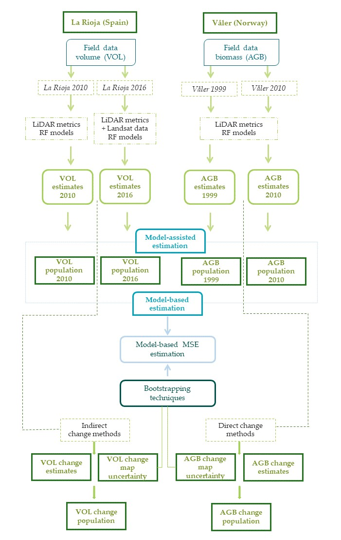
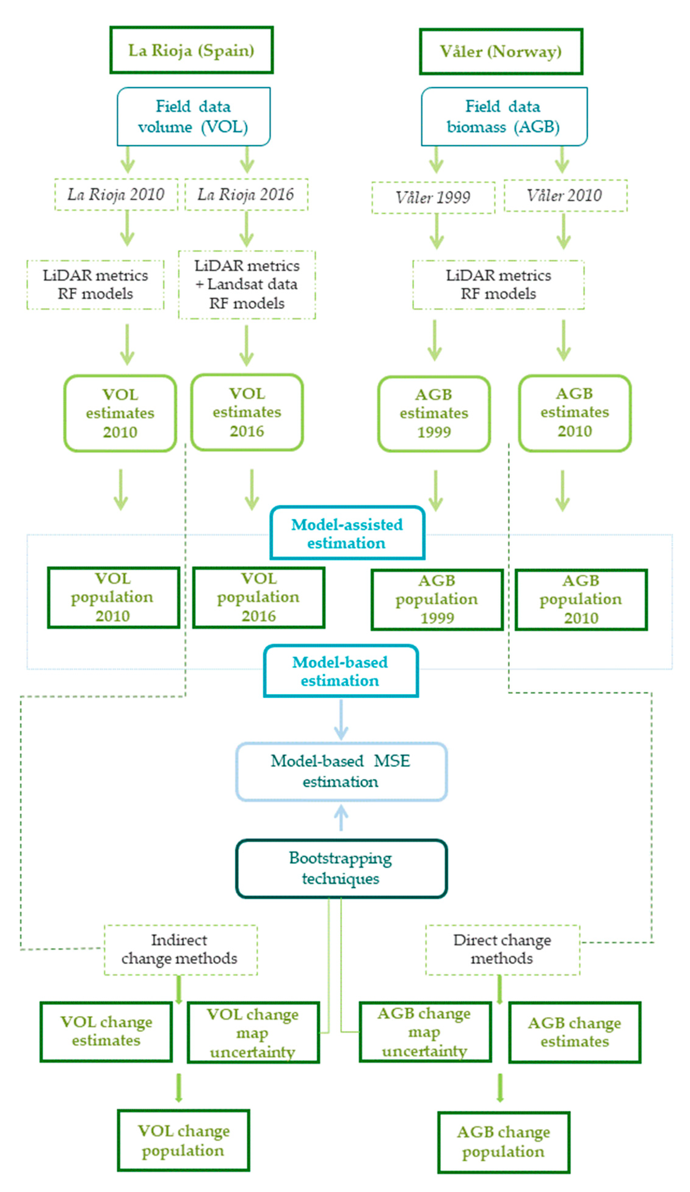
2.6. Overall Workflow

A flowchart depicting the steps conducted in this study and previously described is presented (Figure 2).

3. Results

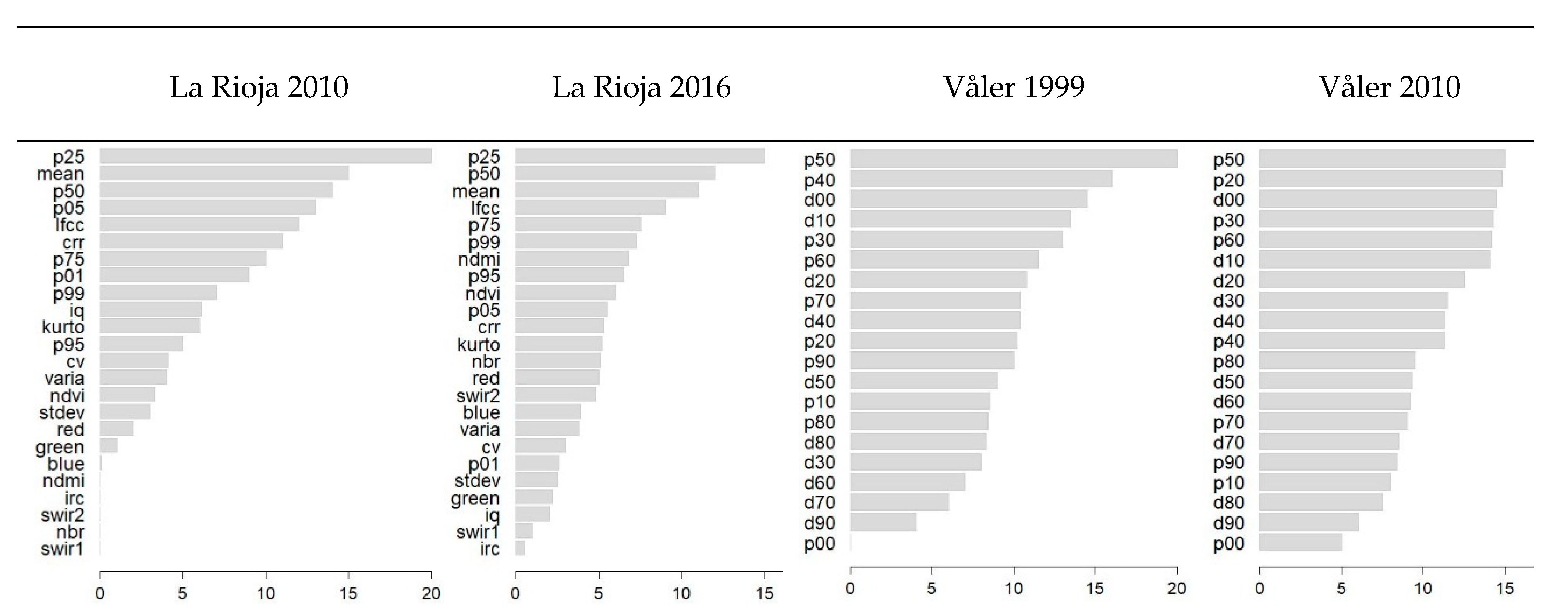
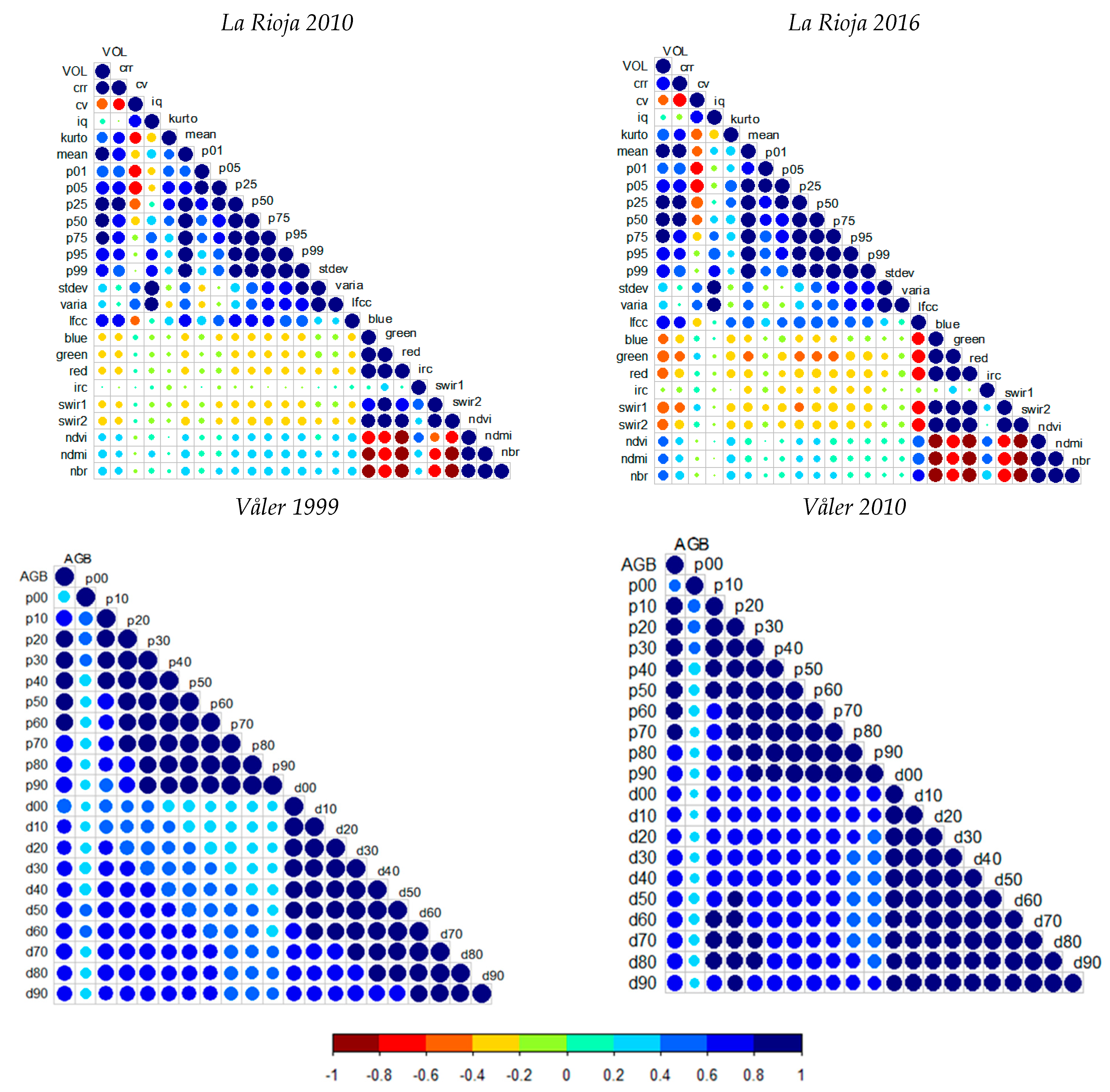
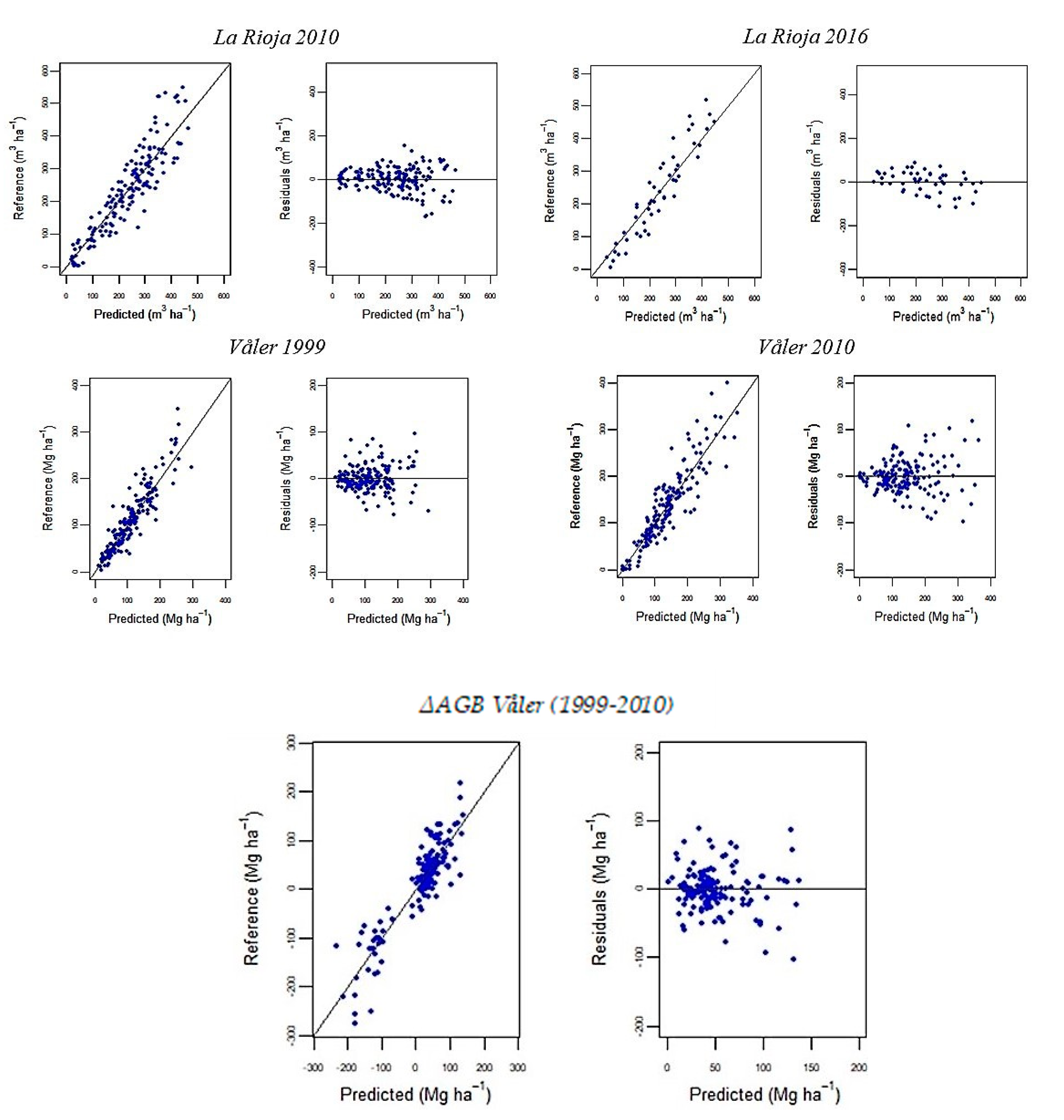
3.1. Random Forests Regression Models

For the La Rioja datasets, RF %IncMSE indicate that the most important variables for both La Rioja datasets were the 25th and 50th percentiles and the ALS height mean (Figure 3). However, because of the large correlations among these variables, only the 25th percentile was used (Figure 4). Overall, all the ALS metrics had large correlations with VOL observations in the sample units (Figure 4) with the exception of var, iq, cv, and stdev. Somewhat smaller correlations between VOL and the Landsat spectral bands and vegetation indices were observed for La Rioja 2010 than for La Rioja 2016. The final models for La Rioja 2010 that used the 25th and 99th percentiles, lfcc and crr as predictor variables and for La Rioja 2016 that used the 25th and 99th percentile, lfcc and ndmi explained 82–86% of the variability.

For the Våler datasets, the 50th ALS height percentile was the most important predictor variable for both datasets. However, similar importance values were observed for the 50th, 20th, 30th, 60th ALS height percentiles and the 00th and 10th canopy densities for Våler 2010. For Våler 1999, the 40th ALS height percentile and the 00th and 10th canopy densities also ranked high (Figure 3). As for La Rioja 2010 and 2016, ALS metrics, with the exception of 0th height percentile, had strong correlations with field AGB with greater correlations for the percentile metrics than for the density metrics (Figure 4). Among all the height percentile metrics, the 20th, 30th, 40th, 50th, and 60th had the greatest correlations with AGB which agrees with the RF variable importance assessments. In fact, for the Våler change analysis the most important predictor variables were the differences in the 20th, 50th, and 30th ALS height percentiles. RF models constructed with the four most important non-collinear predictor variables explained less variability than when using all ALS metrics. Therefore, AGB and ΔAGB models were fitted using all the ALS metrics. The latter biomass models explained 83–86% of the variability for AGB and 82% of the variability for ΔAGB.

3.2. Estimates of Population Parameters for Each Point in Time

The Exp estimators produced similar estimates of means for La Rioja 2010 and for La Rioja 2016; for the former, ${\widehat{\mu }}_{Exp}$ = 234.74 m³/ha with $SE\left({\widehat{\mu }}_{Exp}\right)=$ 10 m³/ha (4.37%), whereas for the latter ${\widehat{\mu }}_{Exp}$ = 236.53 m³/ha with $SE\left({\widehat{\mu }}_{Exp}\right)=$ 19.34 m³/ha (8.17%) (

Table 2. Population estimates for both study areas.

Estimate	La Rioja 2010	La Rioja 2016	Våler 1999	Våler 2010
${\widehat{\mu }}_{Exp}$	234.74 *	236.53 a	112.40	131.15
$SE\left({\widehat{\mu }}_{Exp}\right)$	10.26 *	19.34 a	5.00	6.94
${\widehat{\mu }}_{MA}$	197.86 *	183.26 a	105.55	119.64
$SE\left({\widehat{\mu }}_{MA}\right)$	4.33 *	7.09 a	2.04	2.6
${\widehat{\mu }}_{MB}$	197.22	183.45	105.83	119.47
${\widehat{\mu }}_{w boot}$	200.15	190.41	113.45	131.35
$SE\left({\widehat{\mu }}_{RF boot}\right)$	6.14	24.88	2.96	3.34
$SE\left({\widehat{\mu }}_{w boot}\right)$	3.5	7.44	1.92	2.25
$SE\left({\widehat{\mu }}_{p boot}\right)$	3.03	7.87	1.82	2.05

Note: RF boot: Pairs bootstrap at internal level; w boot: Wild bootstrap; and p boot: Pairs bootstrap. ^a Reported only for comparative purposes because the sampling design was not probabilistic. * Considered as a probabilistic sampling design in spite of the filtering operations that were undertaken and discarded sample units from the probability sample.

). Differences in ${\widehat{\mu }}_{Exp}$ for the Våler datasets were greater than for the La Rioja datasets, although so was the elapsed time; for Våler 1999, ${\widehat{\mu }}_{Exp}$ = 112.40 Mg/ha with $SE\left({\widehat{\mu }}_{Exp}\right)$ = 5.00 Mg/ha (4.45%) and for Våler 2010, ${\widehat{\mu }}_{Exp}$ = 131.15 Mg/ha with $SE\left({\widehat{\mu }}_{Exp}\right)=$ 6.94 Mg/ha (5.29%). $SE\left({\widehat{\mu }}_{Exp}\right)$ were calculated as proportions of estimates of the respective ${\widehat{\mu }}_{Exp}$. However, because ${\widehat{\mu }}_{Exp}$ for La Rioja 2016 was not based on a probability sample, it is reported only for comparison purposes.

The MA estimates of the means for both study areas were very similar to but smaller than the Exp estimates, especially for La Rioja 2010 and 2016 (Table 2). In all cases, introduction of the remotely sensed auxiliary variables for use with the MA estimators reduced the SEs with $SE\left({\widehat{\mu }}_{MA}\right)$ = 4.33 m³/ha (2.19%) and $SE\left({\widehat{\mu }}_{MA}\right)=$ 4.33 m³/ha (3.87%) for La Rioja 2010 and La Rioja 2016, respectively, and $SE\left({\widehat{\mu }}_{MA}\right)=$ 2.04 m³/ha (1.93%) and $SE\left({\widehat{\mu }}_{MA}\right)=$ 2.6 m³/ha (2.17%) for Våler 1999 and Våler 2010, respectively. As for the Exp estimates, because neither ${\widehat{\mu }}_{MA}$ nor CF for La Rioja 2016 were based on a probability sample, they are reported only for comparison purposes. The CFs or bias estimates for the MA estimator were less than 1% for each dataset and study area: −0.64 m³/ha and 0.19 m³/ha for La Rioja 2010 and La Rioja 2016, and 0.28 Mg/ha and 0.17 Mg/ha for Våler 1999 and Våler 2010. These small bias estimates, which are equivalent to the mean residual, reflect the quality of fit of the RF models to the data and consequently the precision of the estimates. In addition, graphs of observations versus predictions (Figure 5) showed most points were located close to the 1:1 line, although there were a few with greater deviations, particularly for smaller and greater prediction ranges. An inherent feature in RF contributes to this phenomenon which is exacerbated by small sample sizes as in La Rioja 2016. The mean for any node will be the mean of the number of sample observations in each node. Therefore, no prediction can be smaller than the smallest sample observation or greater than the greater sample observation.

External bootstrapping produced SEs that were smaller than internal bootstrap SEs by factors ranging from 1.63 to 3.03. At the external level, the two bootstrap approaches produced similar SEs, albeit slightly smaller for the pairs bootstrap (Table 2). However, smaller should not be construed to indicate more accurate; in particular, because wild bootstrapping mimics the structure of the original sample, which the pairs bootstrapping does not for systematic samples, wild bootstrapping was considered the most reliable. For La Rioja 2010, $SE\left({\widehat{\mu }}_{w boot}\right)=$ 3.5 m³/ha (1.77%); for La Rioja 2016, $SE\left({\widehat{\mu }}_{w boot}\right)=$ 7.44 m³/ha (4.06%); for Våler 1999, $SE\left({\widehat{\mu }}_{w boot}\right)=$ 1.92 Mg/ha (1.81%); and for Våler 2010, $SE\left({\widehat{\mu }}_{w boot}\right)=$ 2.25 Mg/ha (1.88%) (Table 2). Although $SE\left({\widehat{\mu }}_{w boot}\right)$ estimates for Våler 1999 and Våler 2010 were almost identical, different results were observed for La Rioja 2010 and La Rioja 2016.

3.3. Estimates of Population Parameters for Change

3.3.1. Estimates of Parameters

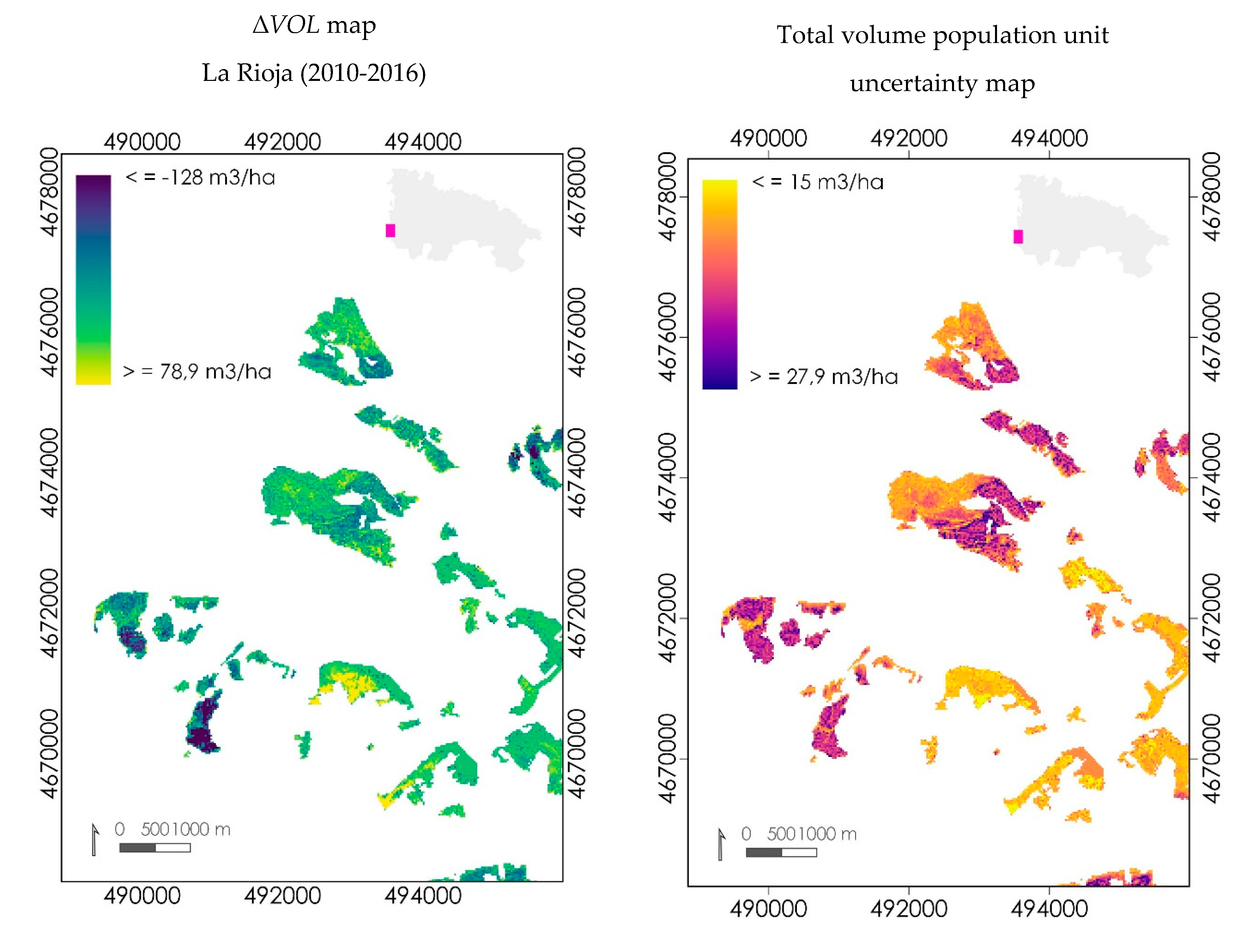
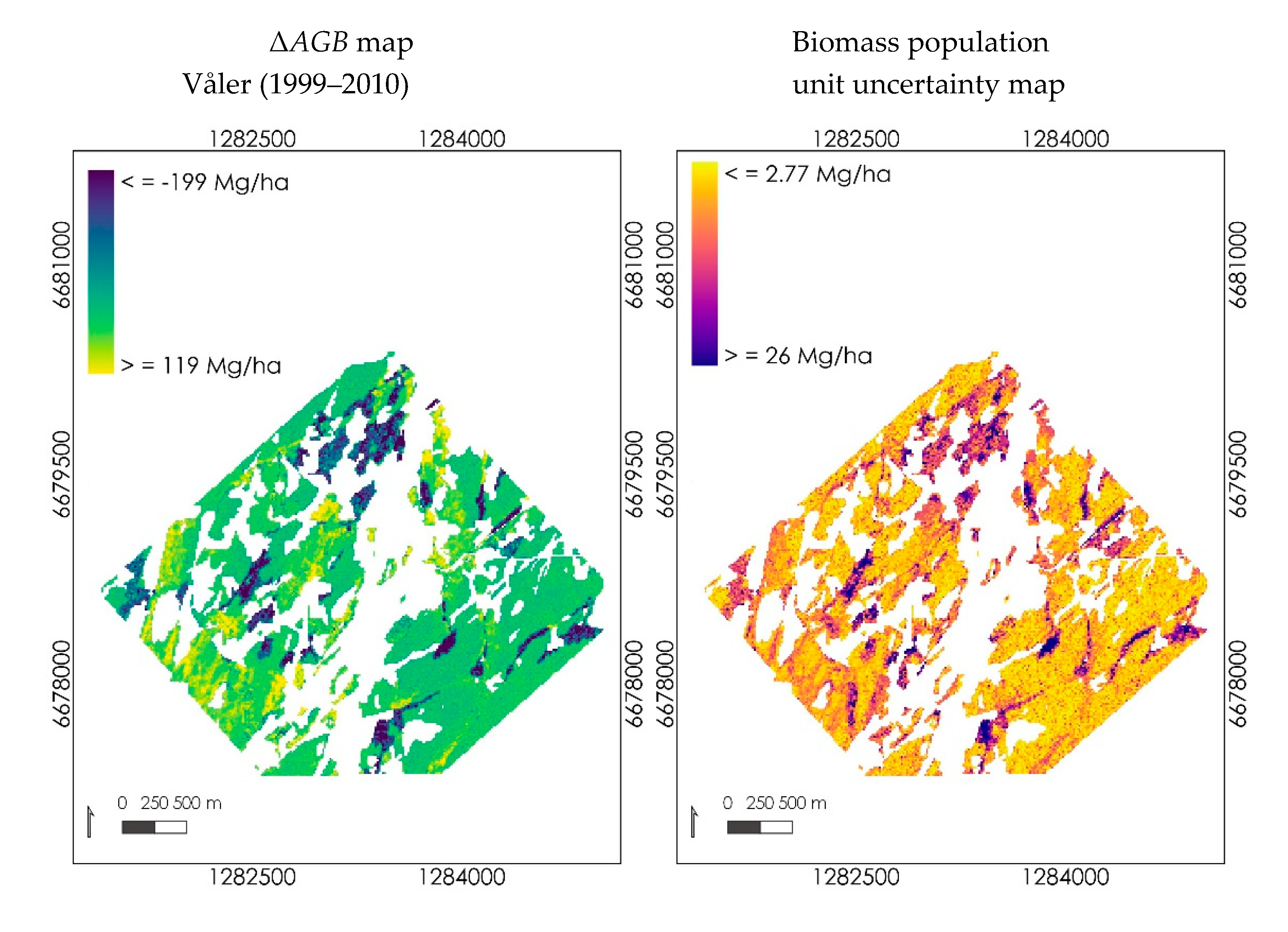
For the La Rioja study area, ΔVOL population unit predictions ranged from −397.43 to 161.31 m³/ha (50% of the population units with negative values) with mean $\overline{\Delta VOL}$ = −10.41 m³/ha and SE ($\overline{\Delta VOL}$) = 8.22 m³/ha. As for the Våler study area, ΔAGB population unit predictions ranged from −230.05 to 163.53 Mg/ha with only approximately 16% of the population units having negative ΔAGB predictions. The model-assisted direct estimate was $\overline{\Delta AGB}$ = 15.11 Mg/ha with SE ($\overline{\Delta AGB}$) = 2.61 Mg/ha (17.27%). The model-based estimate was $\overline{\Delta AGB}$ = 17.02 Mg/ha with SE ($\overline{\Delta AGB}$) = 2.3 Mg/ha (13.51%).

3.3.2. Mapping

Figure 6 shows the change maps for each study area along with their wall-to-wall uncertainty maps. Cold colors (blue) indicate a loss of VOL or AGB while warm colors (yellow) indicate an increase in the reported variables. Greater uncertainty values are associated with the greatest change predictions. For the La Rioja study area, population units with negative ΔVOL predictions coincide with areas where management practices such as clear-cutting or thinning were conducted. Overall, there has been an increased in AGB in the Våler study area and the population units with negative ΔAGB predictions coincide with the deforestation activities classified in McRoberts et al. [46].

4. Discussion

4.1. RF Optimitation: Landsat Variables

Even though SNFI plots are characterized by the lack of precision for plot center coordinates, the RF models adequately described the relationship between the plot-level VOL observations and the remotely sensed data resulting in smaller SE estimates. Nevertheless, for future analysis SNFI plot and ALS cell sizes should be the same. The differences between the Exp and the MA estimates for La Rioja 2010 and for La Rioja 2016 might be due to differences in the sample and population distributions of the auxiliary variables [35]. As shown in

Table 3. Ranges of the auxiliary variables in the sample and the population (Pop) for La Rioja 2010 and La Rioja 2016.

Dataset	Measure	Auxiliary Variable
		p25		p99		crr		lfcc
		Sample	Pop	Sample	Pop	Sample	Pop	Sample	Pop
La Rioja 2010	Mean	8.28	7.03	14.80	13.19	0.54	0.49	79.93	64.67
	Min	2.40	0.00	4.51	0.00	0.25	0.00	7.79	0.00
	Max	16.62	38.75	27.26	44.72	0.76	0.88	100	100
	Range	14.22	38.75	22.75	44.72	0.51	0.88	92.21	100
		p25		p99		ndmi		lfcc
		Sample	Pop	Sample	Pop	Sample	Pop	Sample	Pop
La Rioja 2016	Mean	9.61	7.52	16.42	14.59	0.29	0.29	69.21	65.36
	Min	2.22	0.00	3.36	0.00	0.06	-0.31	7.63	0.00
	Max	17.27	39.23	24.92	44.58	0.48	0.79	99.93	100
	Range	15.05	39.23	21.56	44.58	0.42	1.1	92.3	100

Note: p25, p99 are the 25th and 99th height percentiles (m), lfcc is the forest canopy cover (%) and ndmi is the normalized difference moisturize index.

, the auxiliary variables for the population units have a greater range than for the sample. Unlike regression models, RF cannot extrapolate beyond the range of the response variable in the sample.

This study demonstrated that the use of remotely sensed auxiliary data led to smaller standard error estimates. Overall, Landsat vegetation indices based on NIR and SWIR bands were the most important variables among optical data in the La Rioja study area. This finding is consistent with Dube and Mutanga [65] who reported that SWIR bands and vegetation indices were most important for predicting AGB. In addition, Condés and McRoberts [31] confirmed that SWIR band and ndvi were the most correlated with volume change. However, none of the optical variables were in the final RF volume model for La Rioja 2010 due to their smaller correlations with the volume variable. This result could be attributed to the less accurate plot center coordinates for La Rioja 2010 resulting in NFI field plot observations that do not exactly match with the corresponding Landsat band values [66]. SNFI plots with complete forest cover could be located in population units that are not completely forested with the result that the Landsat reflectance signal for the plot could be mixed with the bare soil reflectance.

4.2. Statistical Inference and Bootstrap Techniques

The novelty of this study resides in the fact that model-based MSE estimation with the RF algorithm is assessed through different bootstrapping approaches. Both the population mean and the MSE of the estimate of the population mean are necessary for inferences for population parameters in the form of confidence intervals. Because RF regression trees are constructed using resamples selected with replacement from the original sample (i.e., pairs bootstrapping), the resample might not mimic the original sample as is required for bootstrapping [33,58,60,61,62]. Further, resampling with replacement may reduce the ranges of the predictor variables, particularly for small samples, thereby introducing bias because of the inability of RF to extrapolate beyond the range of the sample or resample data. These features could contribute to greater SEs when the internal bootstrapping pairs is used, as was observed in La Rioja 2016, although greater SEs were only observed when Landsat variables were included. When only the ALS metrics for La Rioja 2016 were used, $SE\left({\widehat{\mu }}_{RF boot}\right)=$ 12.13 m³/ha as opposed to $SE\left({\widehat{\mu }}_{RF boot}\right)=$ 24.88 m³/ha. In this study, because the RF models were constructed with only four predictor variables, only a single variable was considered by the algorithm for splitting a node. Many of those nodes could have been split with the less-correlated predictor variable (ndmi) with the response VOL variable among all the predictor variables with which the RF model was constructed. This could lead to greater loss of volume prediction precision, and thereby, greater MSE estimates. These findings lead us to exercise caution if internal pairs bootstrapping procedures are used to estimate the model-based MSE. Because model-based MSE estimates were smaller when pairs bootstrapping was used at both internal and external levels, further work should be directed to the wild bootstrapping approach at both internal and external levels.

The greater $SE\left({\widehat{\mu }}_{w boot}\right)$ for La Rioja 2016 could be attributed to the smaller calibration data set size used [20,39]. Nevertheless, even though the sampling intensity in La Rioja 2016 was smaller by a factor of 3 compared to La Rioja 2010, the SE differences were not meaningful. Model-based SEs depend not only on sample size but also on the model, the model estimates, the covariance for the model estimates, and values of independent variables [24]. This suggests that little may be lost by using a smaller purposively selected calibration data set. This feature is an appealing option for conducting forest inventories in remote areas where the acquisition of field data for probability sampling designs may be prohibitive, either for economic or logistic reasons. Reduction in field-plot sample sizes could allow more money for remotely sensed data acquisition whose integration leads to greater precision in estimates. Alternatively, RF models for La Rioja 2010 could be temporally transferred to the La Rioja 2016 ALS data, thereby capitalizing on the greater SNFI sampling intensity and the greater point density of the 2016 ALS data [16,67]. However, the effectiveness of the RF model based on earlier data could depend on the particular forest attribute predicted and the differences between point cloud characteristics for the ALS data used to construct the model and the ALS data used when applying the model [68]. Tompalski et al. [68] observed up to 6% differences in mean predicted volume when ALS data of different pulse densities were used. Besides point density, other factors related to flight design or sensor configuration can affect the main forest variables estimation at least as much as differences in pulse densities [69]. Nationwide flight campaigns cover a wide range of forest types and topographic structures, with highly variable and not always optimal flying conditions. Holmgren et al. [70] found that canopy cover was more affected by scanning angle than laser height percentiles and Montaghi [71] indicated that most plot-level prediction metrics were relatively unaffected by high scanning angles, up to 20 degrees. Furthermore, the effects of climate change could change the natural conditions between the data acquisition dates and compromise the effectiveness of an RF model constructed using earlier data [72].

4.3. Population Change

A large number of studies have demonstrated the value of multi-temporal ALS data for estimating changes in forest attributes [12,16,73]. Change maps are important for understanding the state and dynamics of forests, and they can be used as an initial information source for reporting carbon emissions. Even though our methodology focuses on a regional area, it could have national implications because it mostly leverages open source data gathered to compile data for a better understanding of the forest status. Numerous countries continue to acquire second coverage ALS data resulting in a greater number of territories with multi-ALS flights in which our workflow could be replicated. The similarity of the results obtained for this study ($\overline{\Delta AGB}$ = 15.11 Mg/ha with SE ($\overline{\Delta AGB}$) = 2.61 Mg/ha (17.27%)) with previous studies on change estimation with remotely sensed data lend support for the suitability of the RF algorithm. Nӕsset et al. [74] and McRoberts et al. [15] analyzed the same Våler data using linear regression models with a direct change approach. The former reported $\overline{\Delta AGB}$ = 11.9 Mg/ha with SE ($\overline{\Delta AGB}$) = 1.6 Mg/ha (13.44%), and the latter $\overline{\Delta AGB}$ = 13.62 Mg/ha with SE ($\overline{\Delta AGB}$) = 2.21 Mg/ha (16.23%). Zhao et al. [14] found similar differences between linear regression models and RF when estimating ΔAGB.

Although direct approaches are often reported as preferable in the scientific literature because only errors from one model are incorporated [12,13,74], other studies have found greater accuracies with indirect methods. Økseter et al. [75] estimated ΔAGB in boreal forest using multi-temporal ALS data in Norway and reported the indirect approach as a more satisfactory. McRoberts et al. [15] showed indirect methods produced greater precision when using nonlinear models with the same Våler data as used for this study. Zhao et al. [14] estimated ΔAGB in a forested landscape in Scotland with the indirect approaches showing slightly more precise performances. In addition, the indirect modeling has been claimed to be less sensitive to extrapolating and it has been found to be a better alternative to estimate changes more accurately at stand-level [73]. In light of the diversity of results, the most accurate and/or precise approach may have to be determined by the data available for each study.

4.4. Data Considerations

Direct approaches require repeated measurements of the same field plots which are not always possible due to economic constraints. Further, changes in sampling protocol or field crews between measurements may complicate comparisons of repeated measurements [76]. Costs associated with indirect approaches could be reduced by predicting forest attributes using models with temporal transferability [16] but bearing in mind that temporal transferability should be conducted carefully as previously mentioned.

Nevertheless, the notion of worldwide, multi-temporal, wall-to-wall ALS data available free of charge is likely unrealistic. A substantial investment is required to acquire ALS data for large forest areas, and subsequent processing requires large data storage capability. Because these factors hinder development of forest inventories based on this technology, other alternatives should be considered to mitigate the costs. The increasing access to satellite images may contribute to development of more cost-efficient forest inventories. Basal area removal has been modeled successfully with RF using repeated measurements of NFI plots and Landsat based disturbance products over a 30-year period [77]. Landsat time series have also been explored for mapping AGB dynamics [78]. An alternative to wall-to-wall ALS data could be acquisition of ALS transects in combination with other optical remotely sensed data to estimate forest attributes in a spatially continuous manner [29,79]. Additionally, due to the increased availability of satellite images, an upscaling approach to integrate remotely sensed data from multiple sources has arisen as a suitable alternative for mapping forest attributes at large scales [20,80].

5. Conclusions

Four main conclusions can be drawn from this study: (1) RF models adequately described the relationship between field plot measurements of volume and biomass per unit area and remotely sensed data; (2) model-assisted and model-based estimators based on RF predictions produced similar estimates of population means and change estimates and smaller mean square error estimates than the expansion estimators, thus indicating the utility of remotely sensed data for enhancing forest inventories; (3) because pairs bootstrapping does not mimic the original sample structure and does not preserve the range of predictor variables, wild bootstrapping for MSE estimation is recommended; and (4) the essence of the RF bootstrapping technique could impact on the model-based MSE estimation when internal pairs bootstrapping techniques are applied. By using multi-temporal ALS data, estimates of change for each study area were obtained. For the La Rioja study area the population volume change mean was −10.41 m³/ha (−26.85, 6.03 m³/ha), whereas for the Våler study area the population biomass change mean was 15.11 Mg/ha (9.89, 17.37 Mg/ha). These results reflect a biomass gain in Våler from 1999 to 2010, while in La Rioja we cannot say whether from 2010 to 2016 there has been a loss or gain in the volume stock of Scots pine forest as the volume change confidence interval contains the zero.

References

1. Barrett, F.; McRoberts, R.E.; Tomppo, E.; Cienciala, E.; Waser, L.T. A questionnaire-based review of the operational use of remotely sensed data by national forest inventories. Remote Sens. Environ. 2016, 174, 279–289. [Google Scholar] [CrossRef]
2. Kangas, A.; Astrup, R.; Breidenbach, J.; Fridman, J.; Gobakken, T.; Korhonen, K.T.; Maltamo, M.; Nilsson, M.; Nord-Larsen, T.; Næsset, E.; et al. Remote sensing and forest inventories in Nordic countries–roadmap for the future. Scand. J. For. Res. 2018, 33, 397–412. [Google Scholar] [CrossRef]
3. McRoberts, R.E.; Tomppo, E.O.; Næsset, E. Advances and emerging issues in national forest inventories. Scand. J. For. Res. 2010, 25, 368–381. [Google Scholar] [CrossRef]
4. Tomppo, E.; Gschwantner, T.; Lawrence, M.; McRoberts, R.E. National Forest Inventories: Pathways for Common Reporting; Springer: Dordrecht, The Netherlands, 2010. [Google Scholar]
5. Maltamo, M.; Næsset, E.; Vauhkonen, J. (Eds.) Forestry Applications of Airborne Laser Scanning. Managed Forest Ecosystems; Springer: Dordrecht, The Netherlands, 2010. [Google Scholar]
6. Næsset, E. Estimating timber volume of forest stands using airborne laser scanner data. Remote Sens. Environ. 1997, 61, 246–253. [Google Scholar] [CrossRef]
7. Næsset, E. Predicting forest stand characteristics with airborne scanning laser using a practical two-stage procedure and field data. Remote Sens. Environ. 2002, 80, 88–99. [Google Scholar] [CrossRef]
8. Nӕsset, E. Airborne laser scanning as a method in operational forest inventory: Status of accuracy assessments accomplished in Scandinavia. Scand. J. For. Res. 2007, 22, 433–442. [Google Scholar] [CrossRef]
9. Gobakken, T.; Næsset, E. Assessing effects of laser point density, ground sampling intensity, and field sample plot size on biophysical stand properties derived from airborne laser scanner data. Can. J. For. Res. 2008, 38, 1095–1109. [Google Scholar] [CrossRef]
10. Holmgren, J. Prediction of tree height, basal area and stem volume in forest stands using airborne laser scanning. Scand. J. For. Res. 2004, 19, 543–553. [Google Scholar] [CrossRef]
11. Maltamo, M.; Eerikäinen, K.; Packalén, P.; Hyyppä, J. Estimation of stem volume using laser scanning-based canopy height metrics. Forestry 2006, 79, 217–229. [Google Scholar] [CrossRef] [Green Version]
12. Næsset, E.; Bollandsås, O.M.; Gobakken, T.; Gregoire, T.G.; Ståhl, G. Model-assisted estimation of change in forest biomass over an 11year period in a sample survey supported by airborne LiDAR: A case study with post-stratification to provide “activity data”. Remote Sens. Environ. 2013, 128, 299–314. [Google Scholar] [CrossRef]
13. Noordermeer, L.; Bollandsås, O.M.; Gobakken, T.; Næsset, E. Direct and indirect site index determination for Norway spruce and Scots pine using bitemporal airborne laser scanner data. For. Ecol. Manag. 2018, 428, 104–114. [Google Scholar] [CrossRef]
14. Zhao, K.; Londo, A.; Suarez, J.C.; Hu, T.; Garcia, M.; Wang, C. Utility of multitemporal lidar for forest and carbon monitoring: Tree growth, biomass dynamics, and carbon flux. Remote Sens. Environ. 2018, 204, 883–897. [Google Scholar] [CrossRef]
15. McRoberts, R.E.; Næsset, E.; Gobakken, T.; Bollandsås, O.M. Indirect and direct estimation of forest biomass change using forest inventory and airborne laser scanning data. Remote Sens. Environ. 2015, 164, 36–42. [Google Scholar] [CrossRef]
16. Domingo, D.; Alonso, R.; de la Riva, J.; Lamelas, M.T.; Rodríguez, F.; Montealegre, A.L. Temporal Transferability of Pine Forest Attributes Modeling Using Low-Density Airborne Laser Scanning Data. Remote Sens. 2019, 11, 261. [Google Scholar] [CrossRef]
17. Saarela, S.; Grafström, A.; Ståhl, G.; Kangas, A.; Holopainen, M.; Tuominen, S.; Nordkvist, K.; Hyyppä, J. Model-assisted estimation of growing stock volume using different combinations of LiDAR and Landsat data as auxiliary information. Remote Sens. Environ. 2015, 158, 431–440. [Google Scholar] [CrossRef]
18. Packalén, P.; Suvanto, A.; Maltamo, M. A Two Stage Method to Estimate Species-specific Growing Stock. Photogramm. Eng. Remote Sens. 2009, 75, 1451–1460. [Google Scholar] [CrossRef]
19. Ståhl, G.; Saarela, S.; Schnell, S.; Holm, S.; Breidenbach, J.; Healey, S.P.; Patterson, P.L.; Magnussen, S.; Næsset, E.; McRoberts, R.E.; et al. Use of models in large-area forest surveys: Comparing model-assisted, model-based and hybrid estimation. For. Ecosyst. 2016, 3, 5. [Google Scholar] [CrossRef]
20. Saarela, S.; Holm, S.; Grafström, A.; Schnell, S.; Næsset, E.; Gregoire, T.G.; Nelson, R.F.; Ståhl, G. Hierarchical model-based inference for forest inventory utilizing three sources of information. Ann. For. Sci. 2016, 73, 895–910. [Google Scholar] [CrossRef] [Green Version]
21. Puliti, S.; Saarela, S.; Gobakken, T.; Ståhl, G.; Næsset, E. Combining UAV and Sentinel-2 auxiliary data for forest growing stock volume estimation through hierarchical model-based inference. Remote Sens. Environ. 2018, 204, 485–497. [Google Scholar] [CrossRef]
22. Ståhl, G.; Holm, S.; Gregoire, T.G.; Gobakken, T.; Næsset, E.; Nelson, R. Model-based inference for biomass estimation in a LiDAR sample survey in Hedmark County, Norway. Can. J. For. Res. 2011, 41, 83–95. [Google Scholar] [CrossRef]
23. Chen, Q.; McRoberts, R.E.; Wang, C.; Radtke, P.J. Forest aboveground biomass mapping and estimation across multiple spatial scales using model-based inference. Remote Sens. Environ. 2016, 184, 350–360. [Google Scholar] [CrossRef]
24. McRoberts, R.E.; Næsset, E.; Gobakken, T. Inference for lidar-assisted estimation of forest growing stock volume. Remote Sens. Environ. 2013, 128, 268–275. [Google Scholar] [CrossRef]
25. Andersen, H.-E.; Reutebuch, S.E.; Mcgaughey, R.J.; D’Oliveira, M.V.; Marcus, V.N.; Keller, M. Monitoring selective logging in western Amazonia with repeat lidar flights. Remote Sens. Environ. 2014, 151, 157–165. [Google Scholar] [CrossRef]
26. McRoberts, R.E.; Næsset, E.; Gobakken, T. Estimation for inaccessible and non-sampled forest areas using model-based inference and remotely sensed auxiliary information. Remote Sens. Environ. 2014, 154, 226–233. [Google Scholar] [CrossRef]
27. Belgiu, M.; Drăguţ, L. Random forest in remote sensing: A review of applications and future directions. ISPRS J. Photogramm. Remote Sens. 2016, 114, 24–31. [Google Scholar] [CrossRef]
28. Breiman, L. Random Forests. Mach. Learn. 2001, 45, 5–32. [Google Scholar] [CrossRef] [Green Version]
29. Matasci, G.; Hermosilla, T.; Wulder, M.A.; White, J.C.; Coops, N.C.; Hobart, G.W.; Zald, H.S.J. Large-area mapping of Canadian boreal forest cover, height, biomass and other structural attributes using Landsat composites and lidar plots. Remote Sens. Environ. 2018, 209, 90–106. [Google Scholar] [CrossRef]
30. Navarro, J.A.; Fernández-Landa, A.; Tomé, J.L.; Guillén-Climent, M.L.; Ojeda, J.C. Testing the quality of forest variable estimation using dense image matching: A comparison with airborne laser scanning in a Mediterranean pine forest. Int. J. Remote Sens. 2018, 39, 4744–4760. [Google Scholar] [CrossRef]
31. Condés, S.; McRoberts, R.E. Updating national forest inventory estimates of growing stock volume using hybrid inference. For. Ecol. Manag. 2017, 400, 48–57. [Google Scholar] [CrossRef]
32. Fortin, M.; Manso, R.; Schneider, R. Parametric bootstrap estimators for hybrid inference in forest inventories. Forestry 2018, 91, 354–365. [Google Scholar] [CrossRef]
33. McRoberts, R.E.; Magnussen, S.; Tomppo, E.O.; Chirici, G. Parametric, bootstrap, and jackknife variance estimators for the k-Nearest Neighbors technique with illustrations using forest inventory and satellite image data. Remote Sens. Environ. 2011, 115, 3165–3174. [Google Scholar] [CrossRef]
34. Hou, Z.; McRoberts, R.E.; Ståhl, G.; Packalen, P.; Greenberg, J.A.; Xu, Q. How much can natural resource inventory benefit from finer resolution auxiliary data? Remote Sens. Environ. 2018, 209, 31–40. [Google Scholar] [CrossRef]
35. McRoberts, R.E.; Næsset, E.; Gobakken, T.; Chirici, G.; Condés, S.; Hou, Z.; Saarela, S.; Chen, Q.; Ståhl, G.; Walters, B.F. Assessing components of the model-based mean square error estimator for remote sensing assisted forest applications. Can. J. For. Res. 2018, 48, 642–649. [Google Scholar] [CrossRef]
36. Alberdi, I.; Cañellas, I.; Vallejo Bombín, R. The Spanish National Forest Inventory: History, development, challenges and perspectives. Pesqui. Florest. Bras. 2017, 37, 361. [Google Scholar] [CrossRef]
37. Álvarez-González, J.G.; Cañellas, I.; Alberdi, I.; Gadow, K.V.; Ruiz-González, A.D. National Forest Inventory and forest observational studies in Spain: Applications to forest modeling. For. Ecol. Manag. 2014, 316, 54–64. [Google Scholar] [CrossRef]
38. McRoberts, R.E.; Moser, P.; Zimermann Oliveira, L.; Vibrans, A.C. A general method for assessing the effects of uncertainty in individual-tree volume model predictions on large-area volume estimates with a subtropical forest illustration. Can. J. For. Res. 2014, 45, 44–51. [Google Scholar] [CrossRef]
39. McRoberts, R.E.; Westfall, J.A. Propagating uncertainty through individual tree volume model predictions to large-area volume estimates. Ann. For. Sci. 2016, 73, 625–633. [Google Scholar] [CrossRef]
40. Valbuena, R.; Mauro, F.; Rodriguez-Solano, R.; Manzanera, J.A. Accuracy and precision of GPS receivers under forest canopies in a mountainous environment. Span. J. Agric. Res. 2013, 8, 1047–1057. [Google Scholar] [CrossRef]
41. Mauro, F.; Valbuena, R.; Manzanera, J.A.; García-Abril, A. Influence of global navigation satellite system errors in positioning inventory plots for treeheight distribution studies. Can. J. For. Res. 2011, 41, 11–23. [Google Scholar] [CrossRef]
42. Crecente-Campo, F.; Rojo-Alboreca, A.; Diéguez-Aranda, U. A merchantable volume system for Pinus sylvestris L. in the major mountain ranges of Spain. Ann. For. Sci. 2009, 66, 808. [Google Scholar] [CrossRef]
43. McGaughey, R.; Forester, R.; Carson, W. Fusing LIDAR data, photographs, and other data using 2D and 3D visualization techniques. Proc. Terrain Data Appl. Vis. Connect. 2003, 28, 16–24. [Google Scholar]
44. Vauhkonen, J.; Maltamo, M.; McRoberts, R.E.; Næsset, E. Chapter 1 Introduction to forestry applications of airborne laser scanning. In Forestry Applications of Airborne Laser Scanning, Concepts and Case Studies; Maltamo, M., Næsset, E., Vauhkonen, J., Eds.; Springer: Dordrecht, The Netherlands, 2014; p. 464. [Google Scholar]
45. Banskota, A.; Kayastha, N.; Falkowski, M.J.; Wulder, M.A.; Froese, R.E.; White, J.C. Forest Monitoring Using Landsat Time Series Data: A Review. Can. J. Remote Sens. 2014, 40, 362–384. [Google Scholar] [CrossRef]
46. McRoberts, R.E.; Næsset, E.; Gobakken, T. Comparing the stock-change and gain–loss approaches for estimating forest carbon emissions for the aboveground biomass pool. Can. J. For. Res. 2018, 48, 1535–1542. [Google Scholar] [CrossRef]
47. Liaw, A.; Wiener, M. Classification and Regression by randomForest. R News 2002, 2, 18–22. [Google Scholar]
48. Royall, R.M.; Herson, J. Robust Estimation in Finite Populations I. J. Am. Stat. Assoc. 1973, 68, 880–889. [Google Scholar] [CrossRef]
49. Valliant, R.; Dorfman, A.H.; Royall, R. Finite Population Sampling and Inference; Wiley: New York, NY, USA, 2000; p. 536. [Google Scholar]
50. Särndal, C.-E.; Swensson, B.; Wretman, J. Model Assisted Survey Sampling; Springer: New York, NY, USA, 2019; p. 694. [Google Scholar]
51. Breidt, F.; Opsomer, J.D. Local Polynomial Regression Estimators in Survey Sampling. Ann. Stat. 2000, 28, 1026–1053. [Google Scholar]
52. Breidt, F.; Opsomer, J. Nonparametric and Semiparametric Estimation in Complex Surveys. In Handbook of Statistics—Sample Surveys: Inference and Analysis; Pfeffermann, D., Rao, C.R., Eds.; North-Holland: Amsterdam, The Netherlands, 2009; Volume 28, pp. 103–120. [Google Scholar]
53. Breidt, F.J.; Opsomer, J.D. Model-Assisted Survey Estimation with Modern Prediction Techniques. Stat. Sci. 2017, 32, 190–205. [Google Scholar] [CrossRef]
54. Lehtonen, R.; Särndal, C.-E.; Veijanen, A. Does the model matter? Comparing model-assisted and model-dependent estimators of class frequencies for domains. Stat. Transit. 2005, 7, 649–673. [Google Scholar]
55. Särndal, C.-E. Combined inference in survey sampling. Pak. J. Stat. 2011, 27, 359–370. [Google Scholar]
56. Zheng, H.; Little, R. Penalized spline nonparametric mixed models for inference about a finite population mean from two-stage samples. Surv. Methodol. 2004, 30, 209–218. [Google Scholar]
57. Liu, R. Bootstrap Procedures under some Non-I.I.D. Models. Ann. Stat. 1988, 16, 1696–1708. [Google Scholar] [CrossRef]
58. Flachaire, E. Bootstrapping heteroskedastic regression models: Wild bootstrap vs. pairs bootstrap. Comput. Stat. Data Anal. 2005, 49, 361–376. [Google Scholar] [CrossRef]
59. Freedman, D.A. Bootstrapping Regression Models. Ann. Stat. 1981, 6, 1218–1228. [Google Scholar] [CrossRef]
60. Diaconis, P.; Efron, B. Computer-Intensive Methods in Statistics. Sci. Am. 1983, 248, 116–130. [Google Scholar] [CrossRef]
61. Carpenter, J.; Bithell, J. Bootstrap confidence intervals: When, which, what? A practical guide for medical statisticians. Stat. Med. 2000, 19, 1141–1164. [Google Scholar] [CrossRef]
62. Ranalli, M.G.; Mecatti, F. Comparing Recent Approaches For Bootstrapping Sample Survey Data: A First Step Towards A Unified Approach. In Proceedings of the Joint Statistical Meeting (JSM), San Diego, CA, USA, 28 July–2 August 2012. [Google Scholar]
63. Mentch, L.; Hooker, G. Quantifying Uncertainty in Random Forests via Confidence Intervals and Hypothesis Tests. J. Mach. Learn. Res. 2016, 17, 1–41. [Google Scholar]
64. McRoberts, R.E. Probability- and model-based approaches to inference for proportion forest using satellite imagery as ancillary data. Remote Sens. Environ. 2010, 114, 1017–1025. [Google Scholar] [CrossRef]
65. Dube, T.; Mutanga, O. Evaluating the utility of the medium-spatial resolution Landsat 8 multispectral sensor in quantifying aboveground biomass in uMgeni catchment, South Africa. ISPRS J. Photogramm. Remote Sens. 2015, 101, 36–46. [Google Scholar] [CrossRef]
66. Woodall, C.W.; Russell, M.; Andersen, H.-E.; Domke, G.M.; Deo, R.K.K. Evaluating the influence of spatial resolution of Landsat predictors on the accuracy of biomass models for large-area estimation across the eastern USA. Environ. Res. Lett. 2018, 13, 0550004. [Google Scholar]
67. Fekety, P.A.; Falkowski, M.J.; Hudak, A.T.; Jain, T.B.; Evans, J.S. Transferability of Lidar-derived Basal Area and Stem Density Models within a Northern Idaho Ecoregion. Can. J. Remote Sens. 2018, 44, 131–143. [Google Scholar] [CrossRef]
68. Tompalski, P.; White, J.C.; Coops, N.C.; Wulder, M.A. Demonstrating the transferability of forest inventory attribute models derived using airborne laser scanning data. Remote Sens. Environ. 2019, 227, 110–124. [Google Scholar] [CrossRef]
69. Næsset, E. Effects of different sensors, flying altitudes, and pulse repetition frequencies on forest canopy metrics and biophysical stand properties derived from small-footprint airborne laser data. Remote Sens. Environ. 2009, 113, 148–159. [Google Scholar] [CrossRef]
70. Holmgren, J.; Nilsson, M.; Olsson, H. Simulating the effects of lidar scanning angle for estimation of mean tree height and canopy closure. Can. J. Remote Sens. 2003, 29, 623–632. [Google Scholar] [CrossRef]
71. Montaghi, A. Effect of scanning angle on vegetation metrics derived from a nationwide Airborne Laser Scanning acquisition. Can. J. Remote Sens. 2013, 39, S152–S173. [Google Scholar] [CrossRef]
72. Hou, Z.; Xu, Q.; McRoberts, R.E.; Greenberg, J.A.; Liu, J.; Heiskanen, J.; Pitkänen, S.; Packalen, P. Effects of temporally external auxiliary data on model-based inference. Remote Sens. Environ. 2017, 198, 150–159. [Google Scholar] [CrossRef]
73. Mauro, F.; Ritchie, M.; Wing, B.; Frank, B.; Monleon, V.; Temesgen, H.; Hudak, A. Estimation of changes of forest structural attributes at three different spatial aggregation levels in Northern California using multitemporal LiDAR. Remote Sens. 2019, 11, 923–954. [Google Scholar] [CrossRef]
74. Nӕsset, E.; Gobakken, T.; Bollandsas, O.M.; Gregoire, T.G.; Nelson, R.; Stahl, G. Comparison of precision of biomass estimates in regional field sample surveys and airborne LiDAR-assisted surveys in Hedmark County, Norway. Remote Sens. Environ. 2013, 130, 108–120. [Google Scholar] [CrossRef] [Green Version]
75. Økseter, R.; Bollandsås, O.M.; Gobakken, T.; Næsset, E. Modeling and predicting aboveground biomass change in young forest using multi-temporal airborne laser scanner data. Scand. J. For. Res. 2015, 30, 458–469. [Google Scholar] [CrossRef]
76. Byrne, J.C.; Strand, E.K.; Eitel, J.U.H.; Martinuzzi, S.; Vierling, L.A.; Falkowski, M.J.; Hudak, A.T. Quantifying aboveground forest carbon pools and fluxes from repeat LiDAR surveys. Remote Sens. Environ. 2012, 123, 25–40. [Google Scholar] [Green Version]
77. Tao, X.; Huang, C.; Zhao, F.; Schleeweis, K.; Masek, J.; Liang, S. Mapping forest disturbance intensity in North and South Carolina using annual Landsat observations and field inventory data. Remote Sens. Environ. 2019, 221, 351–362. [Google Scholar] [CrossRef]
78. Pflugmacher, D.; Cohen, W.B.; Kennedy, R.E.; Yang, Z. Using Landsat-derived disturbance and recovery history and lidar to map forest biomass dynamics. Remote Sens. Environ. 2014, 151, 124–137. [Google Scholar] [CrossRef]
79. Ahmed, O.S.; Franklin, S.E.; Wulder, M.A.; White, J.C. Characterizing stand-level forest canopy cover and height using Landsat time series, samples of airborne LiDAR, and the Random Forest algorithm. ISPRS J. Photogramm. Remote Sens. 2015, 101, 89–101. [Google Scholar] [CrossRef]
80. Durante, P.; Martín-Alcón, S.; Gil-Tena, A.; Algeet, N.; Tomé, J.L.; Recuero, L.; Palacios-Orueta, A.; Oyonarte, C. Improving Aboveground Forest Biomass Maps: From High-Resolution to National Scale. Remote Sens. 2019, 11, 795. [Google Scholar] [CrossRef]
Figure 1. Spanish and Norwegian study areas (small map to the right). Location of sample units in the La Rioja study area (large map to the left). ETRS89/UTM zone 30 N (N-E) (EPSG: 3,042).
Remotesensing 11 01944 g001
Figure 2. General methodology workflow used for estimating volume and biomass per unit area as well as the changes in these forest attributes using random forests and remotely sensed data. Note: MSE: Mean square error.
Remotesensing 11 01944 g002
Figure 3. Random forests (RF) variable importance. Note: Height percentiles (ranging from the 0th to 99th percentile: p00, p01, …, p95 and p99); canopy densities (ranging from the 0th to 90th canopy density: d00, d10, …, d90); lfcc: Forest canopy cover; varia: Variance; stdev: Standard deviation; kurto: Kurtosis; iq: Interquartile range; cv: Variation coefficient; crr: Canopy relief ratio; Landsat individual bands (blue, green, red, near infrared (irc) and two shortwave infrared (swir1 and swir2) ndvi: Normalized difference vegetation index; nbr: Normalized burn ratio; and ndmi: Normalized difference moisture index.
Remotesensing 11 01944 g003
Figure 4. Correlation among dependent and independent variables. Note: Height percentiles (ranging from the 0th to 99th percentile: p00, p01, p05, …, p99); canopy densities (ranging from the 0th to 90th canopy density: d00, d10, …, d90); lfcc: Forest canopy cover; varia: Variance; stdev: Standard deviation; kurto: Kurtosis; iq: Interquartile range; cv: Variation coefficient; crr: Canopy relief ratio; Landsat individual bands (blue, green, red, near infrared (irc) and two shortwave infrared (swir1 and swir2) ndvi: Normalized difference vegetation index; nbr: Normalized burn ratio; and ndmi: Normalized difference moisture index.
Remotesensing 11 01944 g004
Figure 5. Observed values versus model predictions for the different RF models in La Rioja (Spain) and Våler (Norway) as well as residuals versus predicted values. Volume observations and volume predictions are shown for the La Rioja study area and biomass observations and biomass predictions for the Våler study area.
Remotesensing 11 01944 g005
Figure 6. The first column provides wall-to-wall change maps and the second one the corresponding uncertainty map. The upper maps show the La Rioja study area and the lower ones the Våler study area. ETRS89/UTM zone 30N (N-E) (EPSG: 3042).
Remotesensing 11 01944 g006aRemotesensing 11 01944 g006b