Thick Cloud Removal in High-Resolution Satellite Images Using Stepwise Radiometric Adjustment and Residual Correction

Abstract

Cloud cover is a common problem in optical satellite imagery, which leads to missing information in images as well as a reduction in the data usability. In this paper, a thick cloud removal method based on stepwise radiometric adjustment and residual correction (SRARC) is proposed, which is aimed at effectively removing the clouds in high-resolution images for the generation of high-quality and spatially contiguous urban geographical maps. The basic idea of SRARC is that the complementary information in adjacent temporal satellite images can be utilized for the seamless recovery of cloud-contaminated areas in the target image after precise radiometric adjustment. To this end, the SRARC method first optimizes the given cloud mask of the target image based on superpixel segmentation, which is conducted to ensure that the labeled cloud boundaries go through homogeneous areas of the target image, to ensure a seamless reconstruction. Stepwise radiometric adjustment is then used to adjust the radiometric information of the complementary areas in the auxiliary image, step by step, and clouds in the target image can be removed by the replacement with the adjusted complementary areas. Finally, residual correction based on global optimization is used to further reduce the radiometric differences between the recovered areas and the cloud-free areas. The final cloud removal results are then generated. High-resolution images with different spatial resolutions and land-cover change patterns were used in both simulated and real-data cloud removal experiments. The results suggest that SRARC can achieve a better performance than the other compared methods, due to the superiority of the radiometric adjustment and spatial detail preservation. SRARC is thus a promising approach that has the potential for routine use, to support applications based on high-resolution satellite images.

1. Introduction

Clouds and the accompanying shadows are inevitable contaminants for high-resolution remote sensing images, which are widely used for urban geographical mapping, land-use classification, change detection [1,2]. According to the estimation of the International Satellite Cloud Climatology Project (ISCCP), the global annual mean cloud cover is as high as 66%. Cloud cover results in missing information and spatio-temporal discontinuity, and thus affects the precise application of time-series satellite images [3]. However, the periodicity of the satellite revisit cycle makes the acquisition of multi-temporal images of a specific region possible. Reconstructing contaminated areas in the cloudy satellite image with the aid of close-date temporal images can help to increase the data usability, and can be used to generate cloud-free and spatio-temporally continuous images for time-series analysis, especially for areas heavily contaminated by clouds. Examples of applications that benefit from cloud removal include land-cover/land-use mapping, change detection, urban planning, etc. Therefore, cloud removal for optical satellite images is of great significance.

In recent years, scholars have undertaken a great deal of research into thick cloud removal for remote sensing images. Considering that thick cloud removal in satellite images is essentially a process of missing information reconstruction [4], thick cloud removal methods can be divided into two main categories, according to the domain of the used complementary information, namely, spatial-based methods and temporal-based methods. We review these two categories of methods in the following.

Spatial-based cloud removal methods use the remaining cloud-free regions in the image to reconstruct the cloud-contaminated regions, without the aid of other auxiliary data. Accordingly, the single-image inpainting approaches can be utilized for the reconstruction of missing regions in an image. Single-image inpainting methods include the commonly used interpolation-based methods [5]; propagated diffusion methods [6], which propagate the local information from the exterior to the interior of the missing areas; variation-based methods [7], which use a regularization technique to implement information reconstruction; and exemplar-based methods [8], which are aimed at reconstructing large missing areas. More relevantly, several recent studies have proposed spatial-based cloud removal methods based on cokriging interpolation [9], bandelet-based inpainting [10], compressive sensing [11], sparse dictionary learning [12], and structure-preserving global optimization [13]. Generally speaking, the spatial-based cloud removal methods can obtain visually plausible results, but they are less effective at coping with large-area clouds and complex heterogeneous areas.

Temporal-based cloud removal methods reconstruct cloud-contaminated regions in the target image based on the complementary information from adjacent temporal images. Since the cloud removal results of the temporal-based methods are usually more reliable than those of the spatial-based methods, especially for removing large-area clouds, the temporal-based cloud removal methods have been more intensively studied. On the one hand, time-series methods reconstruct cloud-contaminated regions by a sliding window filter, function-based curve fitting, etc., and are commonly utilized for the time-series reconstruction of normalized difference vegetation index (NDVI) data [14,15,16], land surface temperature (LST) data [17], and surface reflectance data [18,19]. Since time-series methods have mainly been developed for images with a high temporal resolution, they are not suitable for high-resolution images, which are usually hard to acquire as monthly or seasonal time-series data with a short time interval. On the other hand, cloud removal methods which involve one or more auxiliary images mine the complementary information from the auxiliary image(s) and reconstruct the cloudy areas in the target image through temporal replacement [20,21,22,23], temporal regression [24,25,26,27,28], temporal learning [29,30,31,32,33], etc. The key to these methods is to ensure radiometric consistency and spatial continuity between the recovered areas and the cloud-free areas. In addition, multi-sensor cloud removal methods have also been investigated in recent studies. These methods utilize optical images of a different sensor [34,35] or synthetic aperture radar (SAR) data [36,37,38] to make up for the lack of available target images, and they enhance the ability to reconstruct areas with land-cover changes. However, multi-sensor cloud removal methods may not be applicable for routine use due to the requirement for acquiring a corresponding auxiliary data source.

While many cloud removal methods have been proposed in recent years, most of them are designed for medium- and low-resolution images, such as Landsat [25,27,39] and Moderate Resolution Imaging Spectroradiometer (MODIS) [40,41], and thus may not be suitable for high-resolution images.

There are several major problems for cloud removal in high-resolution images. On the one hand, radiometric consistency between the reconstructed areas and cloud-free areas is difficult to preserve, due to the significant radiometric variations and the dynamic land-cover changes existing between multi-temporal high-resolution images, which brings more challenges for the seamless reconstruction of cloud-contaminated areas. On the other hand, the cloud removal results for high-resolution images are easily affected by noise or artifacts, which leads to missing spatial details, as spatial details in high-resolution images are usually more complex. This results in the actual ground details below the clouds in contaminated imagery being difficult to accurately recover, especially for images covered by large-area clouds.

In this paper, in order to improve the cloud removal results in high-resolution images, we propose a cloud removal method based on stepwise radiometric adjustment and residual correction (SRARC). The basic idea of SRARC is that the complementary information in adjacent temporal satellite images can be utilized for the reconstruction of cloud-contaminated areas in the target image through precise radiometric adjustment, which is achieved by stepwise adjustment and residual correction. The SRARC method has the advantage of being able to preserve the spatial details and radiometric consistency in the reconstructed areas. The experimental results suggest that SRARC is a promising approach, especially for cloud removal in high-resolution satellite images, which will benefit the applications based on high-resolution satellite images, such as large-scale urban mapping.

The rest of this paper is organized as follows. Section 2 introduces the proposed SRARC method and provides the implementation details. The performances of SRARC and the compared methods are evaluated in Section 3, in which images with different resolutions and land-cover change patterns are considered. The parameter settings in SRARC are also analyzed, as well as the efficiency of the different methods. In Section 4, we discuss the superiority and limitations of SRARC. Our conclusions are drawn in Section 5.

2. Method

The inputs of the SRARC method are a target image which is contaminated by cloud, an auxiliary image which is an adjacent temporal image that covers the same area as the target image, and cloud masks of the target image and auxiliary image, which are used as the guidance for the subsequent cloud removal. The masks can be acquired by the existing cloud detection techniques or manual labeling, in which cloud shadow can also be included and finally removed as cloud. In this paper, the acquired target and auxiliary images have already been geometrically registered, and we assume that the regions which are contaminated by clouds in the target image are cloud-free in the auxiliary image. Please note that cloud regions in the target image will not be removed if there is no available cloud-free complementary information in the auxiliary images.

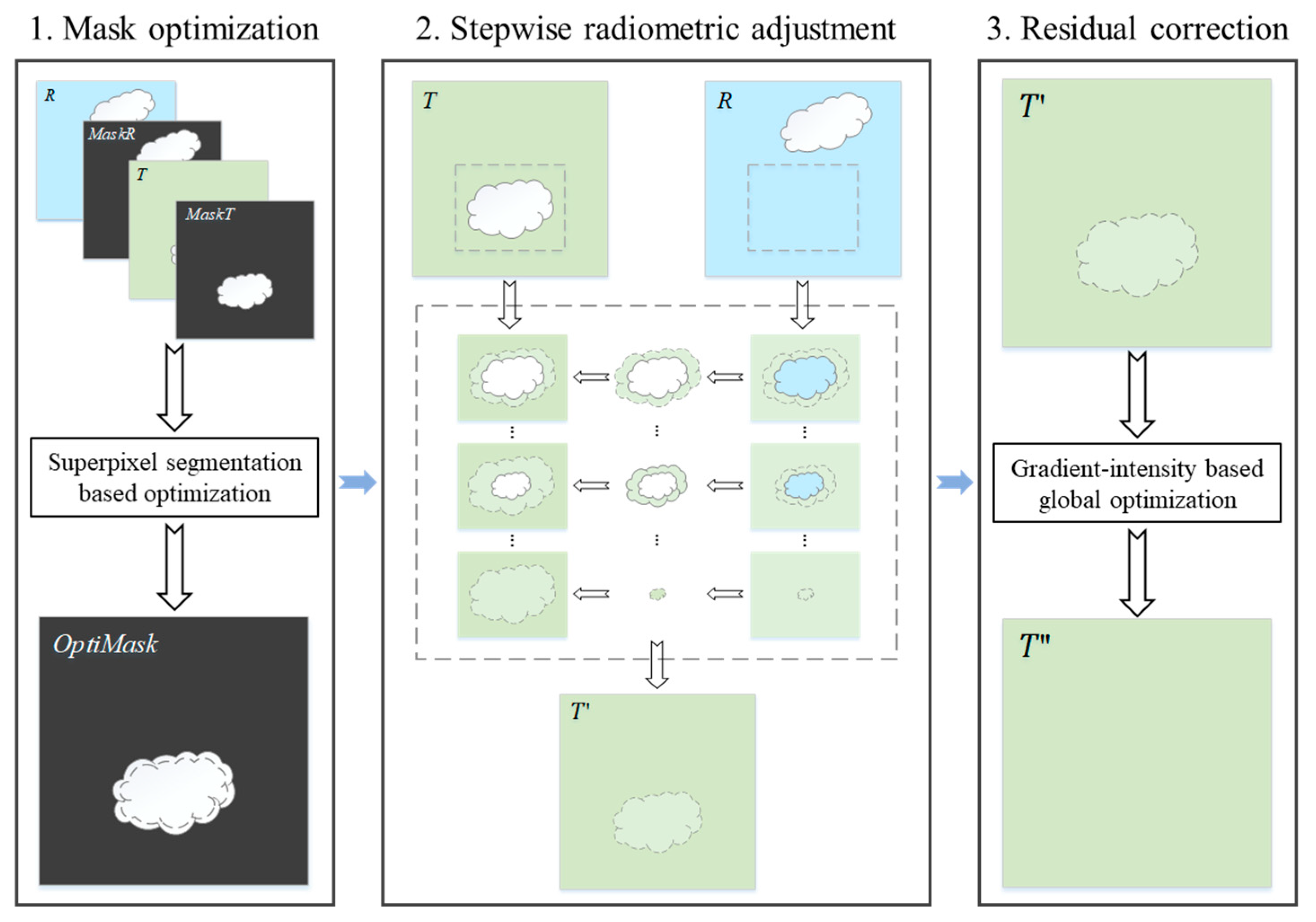
The proposed SRARC method consists of three main steps, as shown in Figure 1. Firstly, the boundaries of the target mask are optimized based on the results of superpixel segmentation, to ensure that they go through homogeneous areas in the target image and avoid spatial discontinuity in the boundaries of recovered areas. The complementary areas from the auxiliary image are then normalized, pixel by pixel, and used to fill the cloud-contaminated areas in the target image, which is achieved by stepwise local radiometric adjustment based on the same cloud-free areas in local windows of the target and auxiliary images. Finally, residual correction is conducted on the filled areas to further eliminate any radiometric differences between the filled areas and the cloud-free areas. The final cloud removal result for the target image can then be generated. For the convenience of the method description in the following subsections, we clipped a pair of experimental images to illustrate the detailed process of SRARC, in which the auxiliary image patch is cloud-free, and we further explain how to cope with the case of the auxiliary image patch also being cloudy.

2.1. Mask Optimization Based on Superpixel Segmentation

Since clouds in the target image are randomly distributed, the boundaries of the labeled clouds in the target mask may also be arbitrarily determined, which can lead to spatial discontinuity in the boundaries of the reconstructed areas. In addition, considering that temporal-based cloud removal is essentially a process of image mosaicing, in which the complementary areas from the auxiliary image are mosaiced to the target image, the optimal seamline is determined by ensuring that it goes through continuous homogeneous areas. Therefore, before the complementary areas are transferred to fill the cloud-contaminated areas in the target image, the boundaries of the target cloud mask should be optimized to ensure the spatial continuity in the reconstruction results, especially for high-resolution images which have complex land structures.

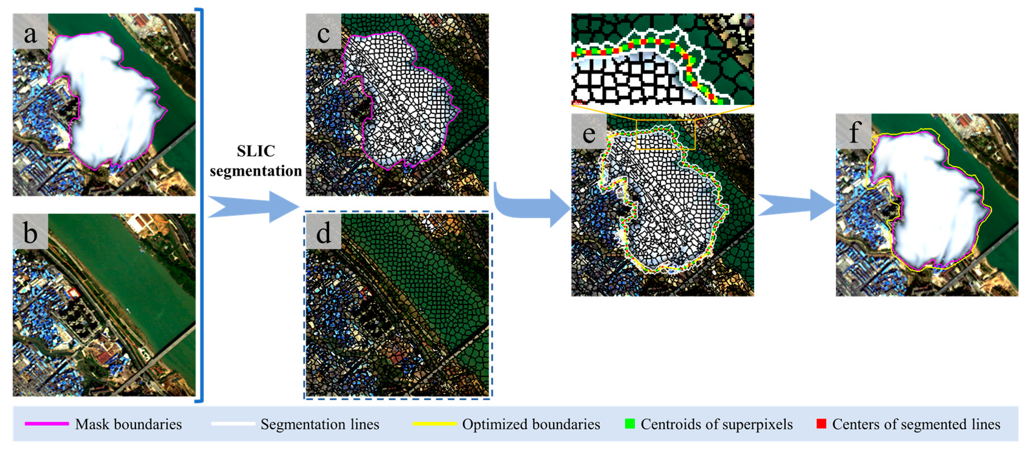
Unlike the seamlines in image mosaicing, the optimized cloud boundaries must form closed areas in the improved cloud mask. In this paper, we optimize the cloud boundaries of the target image by ensuring that they cross the regions of segmented superpixels around the initial cloud boundaries, each of which can be regarded as a local homogeneous region. Since land-cover changes may occur between the cloud-contaminated target image and the auxiliary image, the superpixel segmentation must consider both images, to ensure that they share the same segmentation results. An example of mask optimization is provided in Figure 2. If we assume that the target image and auxiliary image are respectively denoted as $T=\left\{t_1,t_2,\dots ,t_n\right\}$ and $R=\left\{r_1,r_2,\dots ,r_n\right\}$, where $n$ is the number of image bands, we stack the two images and denote this as $TR=\left\{t_1,t_2,\dots ,t_n,r_1,r_2,\dots ,r_n\right\}$. The stacked image $TR$ is then utilized for superpixel segmentation with the simple linear iterative clustering (SLIC) algorithm [42], which is effective and easy to implement. The SLIC algorithm generates superpixels by applying k-means clustering, in which the spatial distance and color differences are both considered to measure the weight distance and cluster local pixels. Specifically, the initial number $N$ of pixels in a superpixel for the segmentation is empirically set to 50, and all the bands in the stacked image are utilized for the segmentation.

The nearest superpixels around cloud boundaries, which are denoted as $S=\left\{s_1,s_2,\dots ,s_m\right\}$, can be acquired by extracting the minimum enclosing segmented lines of cloudy areas. Accordingly, the optimized cloud boundaries can be acquired by connecting the $m$ centroids of $S$ and the $m$ centers of shared segmented lines of $S$. Specifically, the centroid of each superpixel can be acquired by calculating its image moment [43], as in the following equation:

$$M_{pq}={\displaystyle \sum }_{x=1}^m{\displaystyle \sum }_{y=1}^n{x}^p{y}^{q}s\left(x,y\right)$$

(1)

where $\left(p+q\right)$ is the order of moment to be calculated; $s\left(x,y\right)$ denotes the binary image bounding the superpixel, which has a size of $m\times n$; and $s\left(x,y\right)=1$ in the region of the superpixel. The centroid of the superpixel can be calculated as follows.

$$X_G=\frac{M_{10}}{M_{00}}, Y_G=\frac{M_{01}}{M_{00}}$$

(2)

Thus, $\left(X_G, Y_G\right)$ are the coordinates of the centroid point of each superpixel. In addition, the center point $\left(X_C, Y_C\right)$ of the shared segmented line of adjacent superpixels can be approximately obtained by calculating the centroid of each shared segmented line. 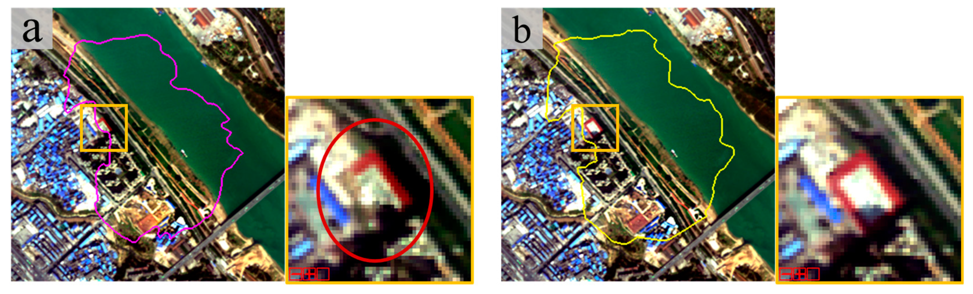The optimized cloud boundaries can be generated by connecting $\left(X_G, Y_G\right)$ and $\left(X_C, Y_C\right)$ of each adjacent superpixel, and according to the formed closed areas, the optimized cloud mask of the target image is acquired. An example comparing the cloud removal results with and without mask optimization is shown in Figure 3, from which we can see that the cloud removal result with mask optimization has better spatial continuity and is more visually plausible.

2.2. Cloud Removal by Stepwise Local Radiometric Adjustment

The stepwise local radiometric adjustment is undertaken to fill cloud-contaminated areas after mask optimization, and is conducted on each cloud region of the target image. For each cloud pixel of each band with coordinates $\left(i,j\right)$ in a cloud region, the target image and auxiliary image in a rectangular window $k$ centered at $\left(i,j\right)$ are used for the normalization to correct the radiation of $R_{\left(i,j\right)}$ and replace the cloud-contaminated pixel $T_{\left(i,j\right)}$ with ${T^{\prime }}_{\left(i,j\right)}$, which can be calculated as follows.

$${T^{\prime }}_{\left(i,j\right)}=\frac{{\sigma }_{T_k}}{{\sigma }_{R_k}}·R_{\left(i,j\right)}+{\mu }_{T_k}-\frac{{\sigma }_{T_k}}{{\sigma }_{R_k}}·{\mu }_{R_k}$$

(3)

where ${T^{\prime }}_{\left(i,j\right)}$ is the recovery result of cloud pixel $T_{\left(i,j\right)}$; ${\sigma }_{T_k}$ and ${\sigma }_{R_k}$ are the standard deviations of the valid cloud-free pixels in window $k$ of the target and the auxiliary image, respectively; ${\mu }_{T_k}$ and ${\mu }_{R_k}$ are the mean values; and the size of window $k$ is $2r+1$, where $r$ is the window radius, which is empirically set to 80 in the stepwise adjustment.

There are several strategies used in the process of stepwise local radiometric adjustment which help SRARC to more effectively cope with the recovery of large-area cloud regions. The details of the strategies are described in the following.

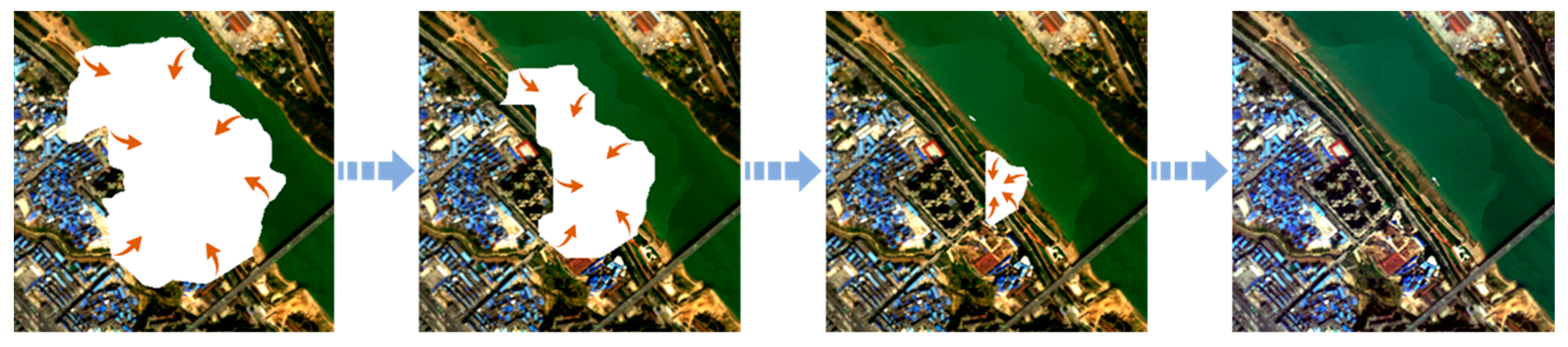
(1) Pixel-by-pixel reconstruction from cloud boundary to center. Since the boundary pixels in cloud regions are closer to the cloud-free pixels and have more reference information for reconstruction, a higher priority for the reconstruction should be set for boundary pixels in cloud regions. Accordingly, in the recovery process of a cloud region, as shown in Figure 4, the recovery order should be from the region boundary to the center, which can be controlled by stepwise one-pixel erosion of the cloud mask until all the cloud pixels have been recovered.

(2) Regarding the recovered pixels of the current cloud region as cloud-free. Instead of increasing the radius of window $k$ to acquire enough valid cloud-free pixels for the recovery of cloud pixels in the center of a large cloud region, the recovered pixels are regarded as valid cloud-free pixels in the reconstruction of the current cloud region, and are utilized for the recovery of the remaining cloud pixels. Such a strategy makes the reconstruction of large-area clouds more effective.

(3) Setting a minimum number of valid pixels for recovery. An insufficient number of valid pixels for normalization in Equation (3) may lead to an unnatural reconstruction result. In SRARC, when the number of involved cloud-free pixels for the recovery of a cloud pixel is less than 30, the recovery is considered as invalid until the condition is met in the following iteration of the stepwise adjustment. Setting a minimum number of valid pixels is beneficial for the reconstruction of cloud pixels around image borders, for which it is usually difficult to find enough valid pixels in the local window.

In the implementation of SRARC, a box filter, which is also called a mean filter, can be utilized to accelerate the calculation of the mean and standard deviation in the local window. Contaminated pixels of each cloud object are recovered by the stepwise local radiometric adjustment, and the initial cloud removal results can then be obtained.

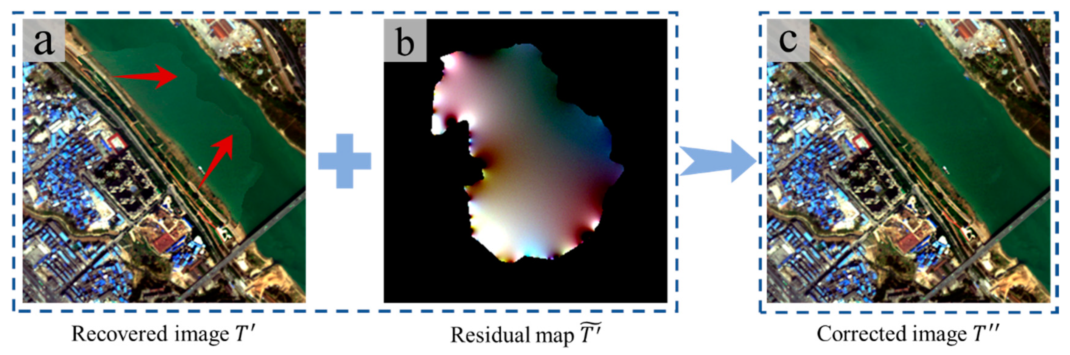
2.3. Residual Correction Through Global Optimization

Since the large radiometric differences have been reduced by the stepwise adjustment, the recovered image will generally have good consistency between the recovered regions and the cloud-free areas. However, due to the limitation of normalization based on local windows, the recovered regions are sometimes not perfectly corrected, and may still be visually inconsistent in the spectral domain, especially for recovered regions containing both land and water areas which have a larger local deviation (see Figure 5a). Therefore, residual correction based on global optimization is utilized to further correct the recovered regions.

We denote the initial recovered image produced by stepwise adjustment as $T^{\prime }$, and the adjusted image after residual correction as $T^{″}$. In order to make $T^{″}$ seamless in the boundaries of the corrected areas (i.e. the recovered areas) while maintaining image details, it is essential to minimize the gradient and intensity differences between $T^{\prime }$ and $T^{″}$ at corrected region $\Omega$, as well as to ensure that the intensities of $T^{\prime }$ and $T^{″}$ are equal at boundaries $\partial \Omega$ of corrected areas. Thus, we should solve the following global optimization problem defined in Equation (4), which includes constraints of the gradient and intensity, and a Dirichlet boundary condition.

$$T^{″}{|}_{\partial \Omega }=argmin{{\displaystyle \iint }}_{\Omega }({|\nabla T^{″}-\nabla T^{\prime }|}^2+\lambda {|T^{″}-T^{\prime }|}^2),T^{″}{|}_{\partial \Omega }=T_{*}^{\prime }{|}_{\partial \Omega }$$

(4)

where $\nabla$ is the gradient operator, $\partial \Omega$ denotes the boundaries of corrected region $\Omega$, and $T_{*}^{\prime }$ is the regions around $\Omega$ in $T^{\prime }$. Note that $\lambda$ is the weight used to balance the fidelity of the gradient and intensity, which is empirically set to a small value to preserve spatial details and spectral information in the residual correction result.

In the study of Pérez et al. [44], only a gradient constraint was used to implement a seamless image clone, which was utilized to reduce the intensity differences after cloning the source image patch to the destination image. In this paper, we additionally introduce the intensity constraint in Equation (4) to better preserve radiometric information in corrected areas, as well as to improve the unnatural results after residual correction in some cases caused by the error propagation from boundaries to the center of the corrected areas [21]. In order to simplify the solving of Equation (4), the above optimization problem is converted into an interpolation problem by introducing the residual term $\widetilde{T^{\prime }}$ and defining the following equation.

$$T^{″}=T^{\prime }+\widetilde{T^{\prime }}$$

(5)

According to Equation (5), Equation (4) can be simplified as follows:

$$\widetilde{T^{\prime }}{|}_{\partial \Omega }=argmin{{\displaystyle \iint }}_{\Omega }({|\nabla \widetilde{T^{\prime }}|}^2+\lambda {|\widetilde{T^{\prime }}|}^2)$$

(6)

The residual term $\widetilde{T^{\prime }}$ at corrected region $\Omega$ can be acquired by solving the Laplace equation with boundary condition, and then $T^{″}$ is obtained according to Equation (5). An example of residual correction is provided in Figure 5.

In addition, considering that the gradients and intensities vary significantly in high-resolution images, the process of residual correction can be iteratively conducted to improve the correction results. The appropriate number of iterations is discussed in the parameter analysis subsection. After the iterative residual correction for each recovered region, the final cloud removal result for the target image can be acquired.

3. Experimental Results and Analyses

In order to evaluate the performance of the proposed SRARC method, we tested SRARC in a series of experiments, in which images with different spatial resolutions and land-cover change patterns were used for the accuracy assessment in both visual and quantitative manners. The compared methods were localized linear histogram match (LLHM) [45], the modified neighborhood similar pixel interpolator (MNSPI) [25], and weighted linear regression (WLR) [26]. Specifically, LLHM is a linear radiometric adjustment method which was originally utilized for gap filling in flawed Landsat Enhanced Thematic Mapper Plus (ETM)+ images, MNSPI combines spectro-spatial information and spectro-temporal information for the prediction of cloudy pixels, and WLR reconstructs missing pixels by weighted linear regression based on local similar pixels. The experiments included both simulated-data experiments and real-data experiments.

3.1. Simulated-Data Experiments

In the simulated-data experiments, the cloud-contaminated target images were simulated by adding simulated thick clouds to the cloud-free images, and the cloud-free images were then considered as the ground truth in the accuracy evaluation. The metrics used to measure the differences between the cloud-removed images and the ground truth for the accuracy evaluation were the correlation coefficient (CC), the root-mean-square error (RMSE), the universal image quality index (UIQI), and the structural similarity (SSIM) index. In addition, the non-reference metric NL (noise level) proposed in [46] for single-image noise level estimation was also utilized for the accuracy evaluation. Note that the accuracies of CC, RMSE, UIQI, and SSIM were calculated based on the recovered areas, while NL was estimated over the whole image. Moreover, the results of SRARC were evaluated over the same recovered areas as the compared methods.

Table 1. Accuracy evaluation results for the simulated cloud removal experiments. The bold values denote the highest accuracies in each experiment, while the underlined values indicate the second-highest accuracies.

	Method	CC (↑)	RMSE (↓)	UIQI (↑)	SSIM (↑)	NL (↓)
Figure 6	LLHM	0.7195	0.0625	0.7054	0.7660	3.60E–03
	MNSPI	0.4551	0.2386	0.4159	0.7624	4.93E–03
	WLR	0.4912	0.3494	0.4651	0.7462	5.96E–03
	SRARC	0.8240	0.0442	0.8228	0.7967	2.04E–03
Figure 7	LLHM	0.7512	0.0537	0.7417	0.7309	5.56E–03
	MNSPI	0.7741	0.0435	0.7604	0.7281	6.21E–03
	WLR	0.8016	0.0410	0.7915	0.7495	5.26E–03
	SRARC	0.8248	0.0408	0.8244	0.7714	4.38E–03
Figure 8	LLHM	0.8789	0.0113	0.8778	0.9599	2.33E–03
	MNSPI	0.9083	0.0093	0.9053	0.9616	2.26E–03
	WLR	0.9077	0.0095	0.9074	0.9618	2.53E–03
	SRARC	0.9195	0.0090	0.9192	0.9642	1.83E–03

lists the quantitative evaluation results for the three simulated cloud removal experiments, and the cloud removal results of the different methods are shown in Figure 6, Figure 7 and Figure 8.

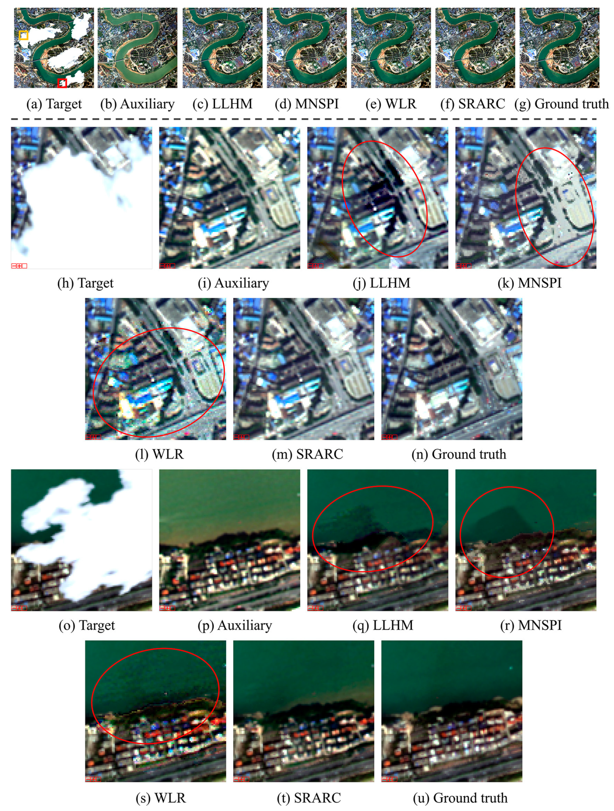
In the first simulated experiment (Figure 6), 4-m resolution Beijing-2 Panchromatic and Multi-Spectral (PMS) images with a size of 1000 × 1000 × 4 over urban and water areas were utilized as the experimental images. Note that significant land-cover changes can observed between the target image and auxiliary image, which were acquired in October 2017 and October 2016, respectively. We can see from the results in Figure 6 that the cloud removal results of LLHM have some color distortion and radiometric inconsistencies in the recovered areas. The results of MNSPI and WLR are heavily affected by the produced noise and artifacts, and thus have a much higher NL than SRARC and much lower CCs of 0.4551 and 0.4912 than SRARC (0.8240), as shown in Table 1. The results of SRARC preserve the details transformed from the auxiliary image and have good spatial-spectral consistency, and thus SRARC achieves the best results, in both the visual and quantitative evaluations.

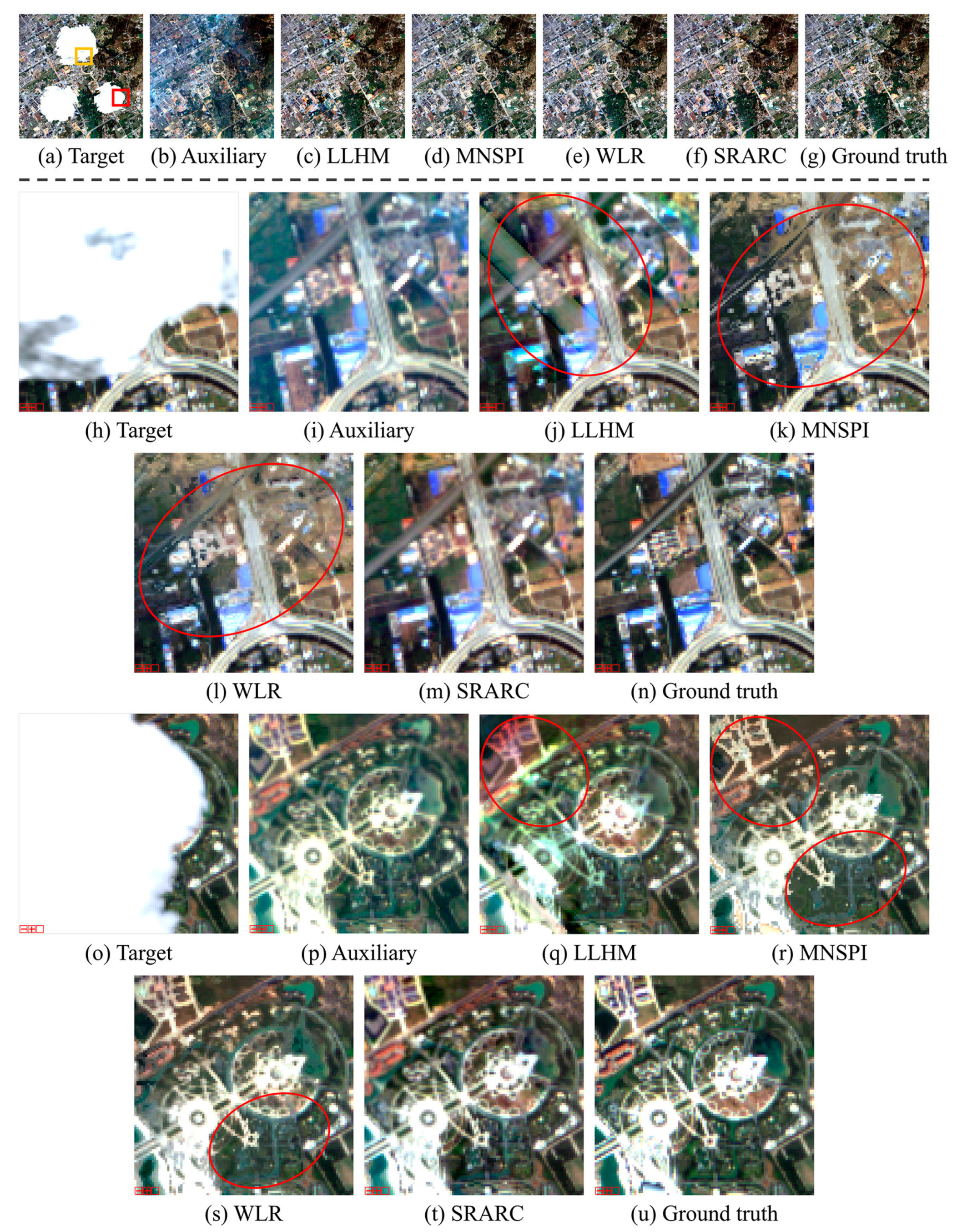
The second simulated experiment (Figure 7) mainly involved phenological changes between the target and auxiliary images, which were derived from 8-m resolution Gaofen-2 PMS images with a size of 800 × 800 × 4. The target and auxiliary images were acquired in April 2016 and December 2015, respectively. The cloud removal results of SRARC and WLR are better than those of LLHM and MNSPI, which have obvious color distortion and artifacts in the recovered areas. Likewise, noise and artifacts occur in the results of WLR, which achieves a UIQI score of 0.7915, which is lower than that of SRARC (0.8244). In this experiment, due to the better radiometric adjustment and detail preserving ability, SRARC generally achieves the most satisfactory results among the different methods.

The temporal gap of the data in the third simulated experiment (Figure 8) was short, and only a few radiometric differences and land-cover changes existed. The target and auxiliary images with a size of 600 × 600 × 4 were derived from four 10-m resolution Sentinel-2 Multispectral Instrument (MSI) bands (three visible bands and a near-infrared band) of urban areas, acquired on September 15, 2018, and September 5, 2018, respectively. In this experiment, the results of all the methods are satisfactory in the visual evaluation, and the acquired quantitative accuracies are much higher than in the first two simulated experiments. Due to the complex land structures in the experimental images, the recovery results of LLH, MNSPI, and WLR are still partially affected by color distortion and noise, while SRARC achieves the best performance among the different methods, confirming the effectiveness of SRARC in cloud removal for high-resolution images under complex land-cover conditions.

3.2. Real-Data Experiments

The real-data experiments were conducted on images covered by real cloud as well as cloud shadow. Two kinds of images with different spatial resolutions were used for the method evaluation in a visual manner. Considering that the cloud removal results of MNSPI were similar to those of WLR in the simulated experiments, and that the public code of WLR is implemented in a more effective manner than MNSPI, only WLR was used for the comparison in the real-data experiments.

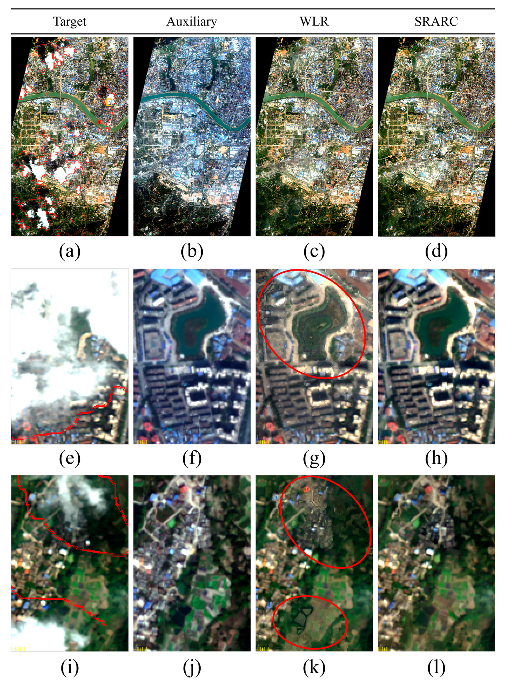
The first real-data experiment was conducted on Beijing-2 PMS images with a 4-m resolution. The cloud-contaminated target image and the cloud-free auxiliary image were acquired on October 9, 2017, and October 11, 2016, respectively, and both contained four NIR-R-G-B bands with a size of 2678 × 4567 × 4. As shown in Figure 9, the red lines in the target image denote the areas of labeled cloud and cloud shadow, and significant radiometric differences can be observed between the target and auxiliary images. Both the WLR and SRARC methods successfully reconstruct the cloud-contaminated areas in the target image, and acquire visually satisfactory results in both homogeneous urban areas and heterogeneous areas which are mainly covered by vegetation. However, obvious noise and artifacts can be observed in the cloud removal result of WLR, while the result of SRARC is clearer in the recovered regions, especially in the complex urban areas, due to the better detail preserving ability.

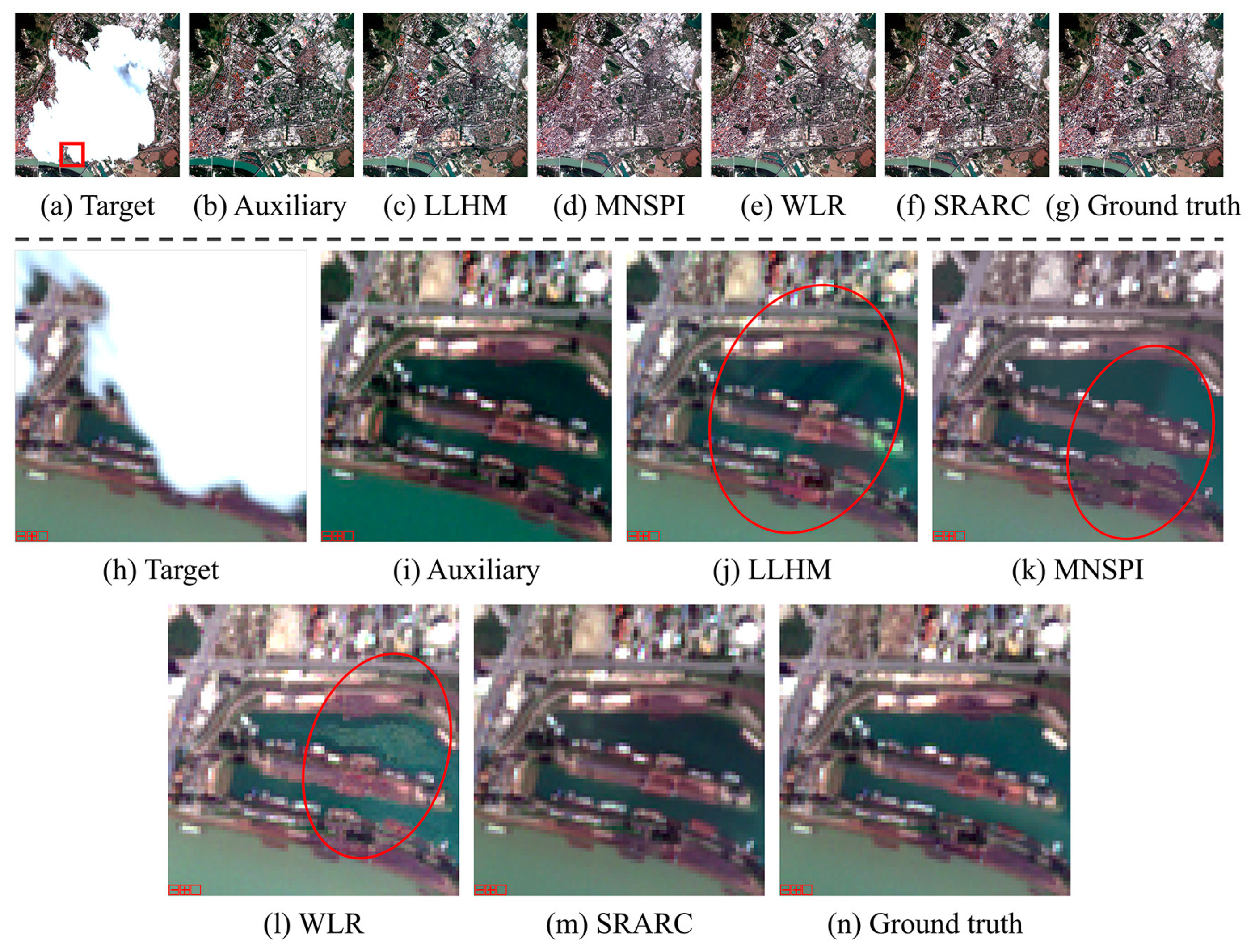
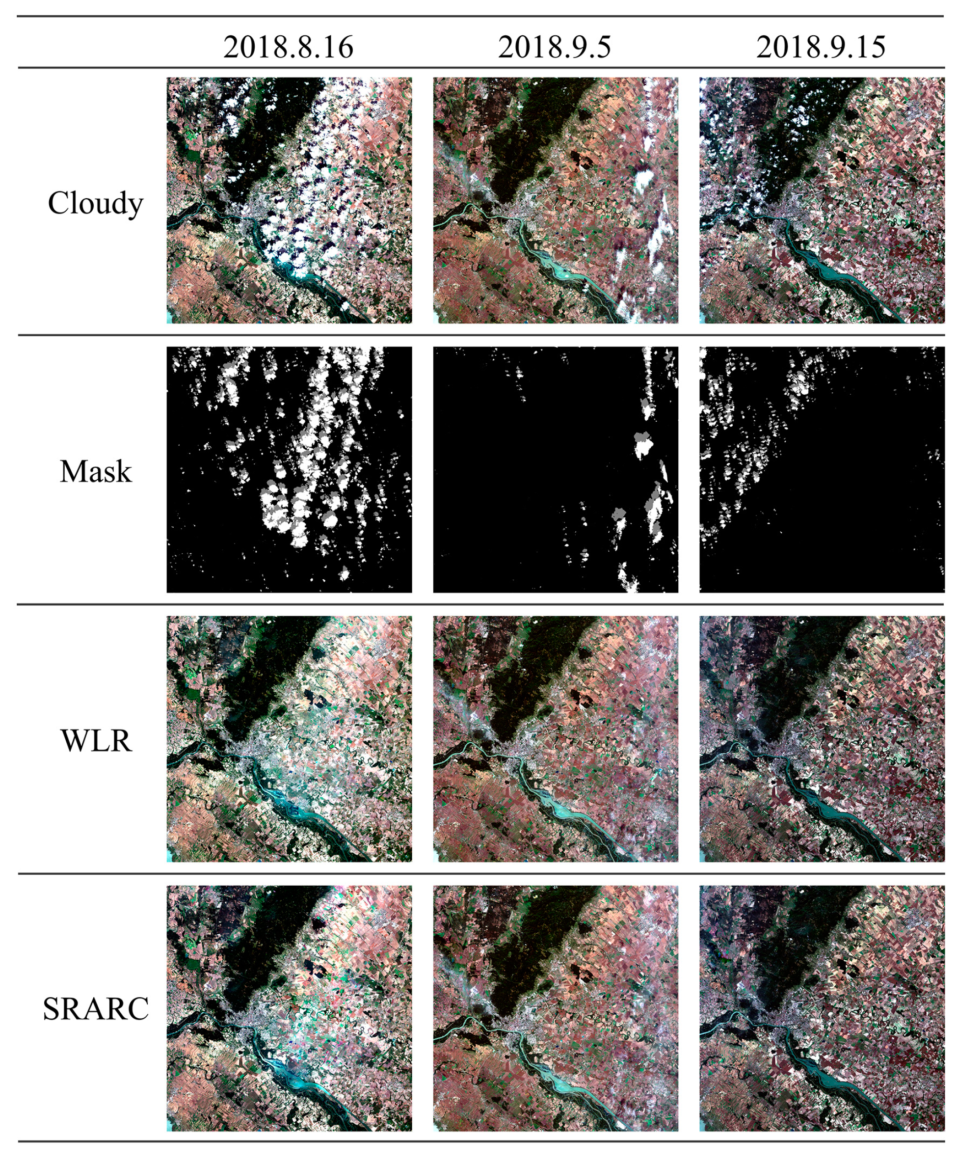
As shown in Figure 10, three temporally adjacent Sentinel-2 MSI images were used in the second real-data experiment, in which all three images were covered by different degrees of cloud cover. The images were acquired on August 16, September 5, and September 15 in 2019. The three images had a size of 7000 × 7000 × 4, and only four 10-m resolution NIR-R-G-B bands were used in the experiment. It can be seen that all the scenes acquired by the satellite imaging system are cloudy, and thus cloud removal based on complementary temporal information is essential to composite clear views of the areas of interest. In this case, cloud and cloud shadow masks of the three images were first automatically generated by a cloud detection method based on multi-scale convolutional feature fusion (MSCFF) [47]. The images acquired on September 5 and September 15 were then used to reconstruct the contaminated areas, based on the complementary information in each image. Finally, the clouds in the image acquired on August 16 were removed using the recovered image acquired on September 5 as the auxiliary image. It can be seen from the results shown in Figure 10 that the thick clouds and cloud shadows in all three images are removed clearly and seamlessly, and only the image acquired on September 5 is partially affected by haze. As shown in Figure 11, the spatial details in the recovered results of SRARC are continuous, whereas noise and artifacts can be observed in the results of WLR, which suggests that the SRARC method is more effective for the removal of large-area clouds.

Note that the superiority of SRARC over WLR is more obvious in this experiment, due to the larger missing areas when combining clouds and cloud shadows, as well as the fact that there is less available complementary information in some areas, as the auxiliary image is also cloudy. Benefiting from the strategies of regarding the recovered pixels of the current cloud region as cloud-free and the pixel-by-pixel reconstruction from cloud boundary to center, SRARC has more advantages when dealing with large-area clouds and cloud shadows than WLR, which recovers cloud pixels completely based on the cloud-free areas and in row-by-row order.

According to the results of the simulated experiments and the real-data experiments under different circumstances, the results of LLHM often contain color distortion, especially when coping with large-area clouds, and the accuracies of MNSPI and WLR are easily affected by the produced noise and artifacts. The three compared methods show their respective advantages with regard to the quantitive accuracy evaluation results in the three groups of simulated experiments. In contrast, we can observe that SRARC is more effective at dealing with different land-cover change patterns, and can acquire high-accuracy cloud removal results which have better radiometric consistency and spatial continuity. Moreover, with the increase of the spatial resolution and the areas of clouds, the superiority of SRARC over the other methods becomes more obvious.

3.3. Parameter Analysis

There are several key parameters in the SRARC method which can affect the reconstruction accuracy for cloud-contaminated areas. In this subsection, the influences of these parameters on the reconstruction accuracy are discussed, and then the recommended parameter settings are given.

The first parameter is the initial number $N$ of pixels in a superpixel for SLIC superpixel segmentation, where a large value of $N$ will result in larger superpixels in the segmentation result. Considering that heterogenous areas in high-resolution images are common, and that larger superpixels are more likely to contain heterogenous pixels, our default setting of $N$ was 50 for the high-resolution images considered in this paper, which can acquire a balanced result between under-segmentation and over-segmentation.

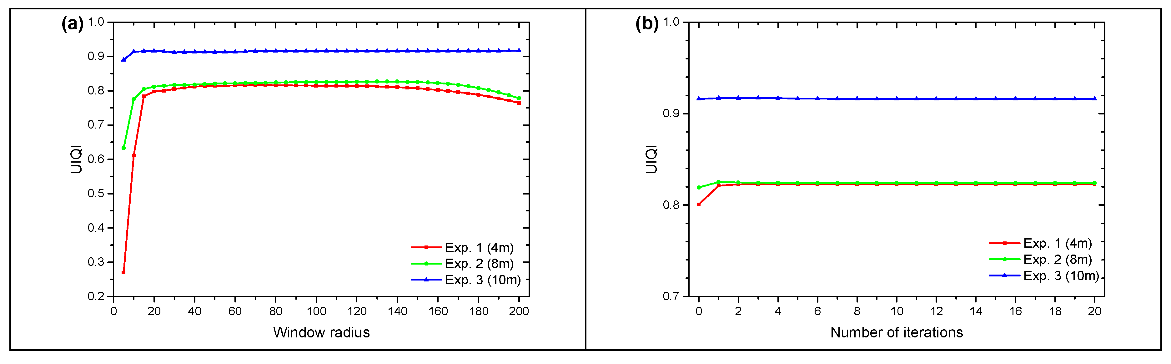
The radius of the window $k$ for the stepwise adjustment affects the results of the radiometric adjustment. Generally speaking, a smaller window radius brings more accurate correction results, but it may also lead to radiometric distortion, especially in areas which have large spectral variations. The most appropriate window radius can be determined by evaluating the reconstruction accuracy with the change of the window radius. According to our evaluation results shown in Figure 12a, which were acquired based on the simulated experiments, a window radius in a range of 20–160 is recommended. Specifically, we empirically set the default window radius as 80 in the stepwise adjustment. Note that the setting of a larger window radius is essential for cloud removal in medium- and low-resolution images.

In the process of residual correction, the iteration number of the residual correction is also related to the reconstruction accuracy of cloud-contaminated areas. The evaluation results shown in 12b reveal that the iteration of the residual correction contributes to the accuracy improvement, whereas the accuracy is slightly reduced when the iteration exceeds a certain threshold. According to our evaluation, three times residual correction achieves the best correction results, and was thus set as the default.

3.4. Efficiency Analysis

Taking the first simulated experiment as an example, in which the cloud-contaminated target image had a size of 1000 × 1000 × 4 and a cloud percentage of 23.44%, we evaluated the efficiency of the proposed method on a laptop with an Intel Core i7-8500U CPU. The repeated test results indicate that SRARC implemented in MATLAB language costs 38.7 seconds to complete the cloud removal under such a situation, which can be considered as satisfactory. Note that the time cost of SRARC is mainly related to the number of cloud-contaminated pixels in the target image, and a slightly longer computation time will be required in cloud removal for fragmentary clouds than for large-area clouds of equal pixels. Furthermore, with the implementation of SRARC using the more effective C/C++ language, the efficiency of SRARC could be further improved.

4. Discussion

Due to the significant spectral variations, abundant spatial details, and dynamic land-cover changes in high-resolution images, the cloud removal methods based on local linear histogram matching usually cannot acquire satisfactory results, in which color distortion occurs in local reconstructed areas, and the results also show radiometric inconsistency. Moreover, the cloud removal results of the methods based on similar pixel regression usually show good radiometric consistency, but they suffer from noise and artifacts in the reconstructed areas, which leads to missing spatial details. As most of the cloud removal methods proposed in the previous studies were developed for medium- and low-resolution images, the results may suffer from radiometric inconsistency and missing spatial details when applying these methods to high-resolution images, resulting in potential errors in the application of the generated cloud-free high-resolution images.

Accordingly, in this paper, we have proposed a thick cloud removal method based on stepwise radiometric adjustment and residual correction (SRARC) for high-resolution images. The SRARC method makes full use of the complementary information from the auxiliary image to recover cloud-contaminated areas in the target image, through a series of steps, including mask optimization, stepwise local radiometric adjustment, and residual correction. Specifically, a mask optimization procedure based on superpixel segmentation is applied to ensure the spatial continuity in the reconstruction results. Moreover, stepwise radiometric adjustment is conducted to reconstruct cloud-contaminated areas, which also preserves spatial details. The minor radiometric differences between the reconstructed areas and cloud-free areas are then eliminated by the following residual correction, finally achieving seamless reconstruction of the cloudy areas. The simulated and real-data experimental results obtained in this study suggest that SRARC is an effective approach that can achieve a better performance than the compared methods in terms of radiometric consistency and spatial continuity, which makes it a promising approach for operational use.

Considering that only the radiometric brightness of the complementary temporal information from the auxiliary image is corrected by SRARC and used to fill the cloud-contaminated areas, cloud-contaminated areas in the target image cannot be accurately recovered under the condition that abrupt land-cover changes have occurred between the target image and auxiliary image. Furthermore, although the strategy of regarding the recovered pixels of the current cloud region as cloud-free in the step of stepwise radiometric adjustment makes SRARC more effective in removing large-area clouds, it may propagate potential error from the previous recovered pixels of the current cloud region. Fortunately, the recovery results for the different cloud regions are free of influence from each other, and the error can be restricted, to some degree, due to the setting of large local window sizes and the use of a minimum number of valid pixels for recovery.

Therefore, as with most of the multi-temporal cloud removal methods proposed previously, SRARC is more suitable for cloud removal in images which have a relatively short temporal interval and no significant land-cover changes. For instance, SRARC could be used to generate high-quality and spatio-temporally continuous satellite images to support high-resolution urban geographical mapping at monthly/seasonal/yearly scales.

5. Conclusions

In this paper, with the aim of improving the cloud removal results in high-resolution satellite images, which often suffer from the problems of radiometric distortion, noise and artifacts, we have proposed a thick cloud removal method based on stepwise radiometric adjustment and residual correction (SRARC). The experimental results reveal that the proposed SRARC method is effective in removing the thick clouds in high-resolution satellite images. As a result of the radiometric adjustment and spatial detail preservation ability, SRARC outperforms the other compared cloud removal methods, suggesting that SRARC has the potential for routine use to support applications based on high-resolution satellite images.

In our future study, multi-source data will be incorporated with the target image to allow the proposed method to better cope with the reconstruction of cloud-contaminated areas suffering significant land-cover changes. Furthermore, the proposed cloud removal method will be applied to generate clear views of desired areas and dates, and to support urban land-use mapping with time-series and high-resolution satellite images.