Semiautomated Detection and Mapping of Vegetation Distribution in the Antarctic Environment Using Spatial-Spectral Characteristics of WorldView-2 Imagery

Abstract

Effective monitoring of changes in the geographic distribution of cryospheric vegetation requires high-resolution and accurate baseline maps. The rationale of the present study is to compare multiple feature extraction approaches to remotely mapping vegetation in Antarctica, assessing which give the greatest accuracy and reproducibility relative to those currently available. This study provides precise, high-resolution, and refined baseline information on vegetation distribution as is required to enable future spatiotemporal change analyses of the vegetation in Antarctica. We designed and implemented a semiautomated customized normalized difference vegetation index (NDVI) approach for extracting cryospheric vegetation by incorporating very high resolution (VHR) 8-band WorldView-2 (WV-2) satellite data. The viability of state-of-the-art target detection, spectral processing/matching, and pixel-wise supervised classification feature extraction techniques are compared with the customized NDVI approach devised in this study. An extensive quantitative and comparative assessment was made by evaluating four semiautomatic feature extraction approaches consisting of 16 feature extraction standalone methods (four customized NDVI plus 12 existing methods) for mapping vegetation on Fisher Island and Stornes Peninsula in the Larsemann Hills, situated on continental east Antarctica. The results indicated that the customized NDVI approach achieved superior performance (average bias error ranged from ~6.44 ± 1.34% to ~11.55 ± 1.34%) and highest statistical stability in terms of performance when compared with existing feature extraction approaches. Overall, the accuracy analysis of the vegetation mapping relative to manually digitized reference data (supplemented by validation with ground truthing) indicated that the 16 semi-automatic mapping methods representing four general feature extraction approaches extracted vegetated area from Fisher Island and Stornes Peninsula totalling between 2.38 and 3.72 km² (2.85 ± 0.10 km² on average) with bias values ranging from 3.49 to 31.39% (average 12.81 ± 1.88%) and average root mean square error (RMSE) of 0.41 km² (14.73 ± 1.88%). Further, the robustness of the analyses and results were endorsed by a cross-validation experiment conducted to map vegetation from the Schirmacher Oasis, East Antarctica. Based on the robust comparative analysis of these 16 methods, vegetation maps of the Larsemann Hills and Schirmacher Oasis were derived by ensemble merging of the five top-performing methods (Mixture Tuned Matched Filtering, Matched Filtering, Matched Filtering/Spectral Angle Mapper Ratio, NDVI-2, and NDVI-4). This study is the first of its kind to detect and map sparse and isolated vegetated patches (with smallest area of 0.25 m²) in East Antarctica using VHR data and to use ensemble merging of feature extraction methods, and provides access to an important indicator for environmental change.

1. Introduction

Parts of Antarctica have experienced major changes in temperature, wind speed, and the impacts of stratospheric ozone depletion since the mid-Twentieth Century [1,2]. The climatic changes are predicted to continue, leading to higher summer temperatures and generally increased water availability in ice-free areas which, in turn, will encourage increased growth and extent of cryospheric vegetation and other biological groups and communities [3]. The distribution of vegetation is influenced by a range of environmental factors including soil moisture, permafrost depth, seasonal temperature, atmospheric CO₂, geomorphology, and ice-free area [4,5,6], with these factors exerting influences at a range of spatial scales [7]. Regardless of Antarctica’s sensitivity to changing climate, few studies have yet addressed in detail the response of Antarctic vegetation to changing climatic conditions [8,9,10,11,12,13]. Baseline information documenting distribution of vegetation is required against which to spatio-temporally monitor changes in extent in response to changing climatic conditions. Therefore, there is a pressing need for the development and application of digital mapping methods capable of generating detailed vegetation maps in this pristine, remote, and inaccessible environment.

In recent years as available technology has advanced, polar researchers have started to employ analytical techniques based on remote sensing (RS) data for mapping polar vegetation in order to address the practical inaccessibility of much cryospheric terrain. Satellite-based optical observations such as the Landsat series and aerial images collected from drones and aircraft using very high resolution (VHR) cameras can play a vital role in revealing vegetation changes occurring in the Antarctic cryosphere over time [14,15,16]. To date, most polar studies on vegetation mapping have focused on Arctic tundra (e.g., [17,18]) due to ease of accessibility, lower logistic costs, and more detectable vegetation (higher plants, e.g., bushes/trees, with larger extent), with comparatively few attempts yet in Antarctica and those that exist being based on validation with limited reference to in-situ data [19]. Mapping vegetation in Antarctica using medium resolution imagery is challenging due to the sparse and patchy nature of vegetation extent [19].

Malenovský et al. [20] developed a non-invasive remote sensing method to assess health of short-stature Antarctic vegetation using a hyperspectral unmanned aircraft system (UAS). Using VHR data from IKONOS, Murray et al. [21] classified the vegetation on Heard Island using a maximum likelihood (MXL) classification, a texture-based classification, and a combination of both. Bricher et al. [16] mapped reliably the endangered plant species Azorella macquariensis using Random Forest (RF) classification and geographic object-based image analysis. Casanovas et al. [22] compared NDVI and matched filtering (MF) approaches for mapping lichens in the Antarctic. However, other important groups of Antarctic vegetation, such as mosses and cyanobacteria, were inadequately detected by MF, providing a further challenge to the effective extraction of vegetation. The sub-pixel supervised classification used by Shin et al. [23] resulted in uncertainties between field survey and pixel areas, time gaps, and spectral characteristics of species.

RS supports the characterization of varying vegetation classes by a spatially scattered pattern of spectral responses, allowing a greater discrimination of classes in various environments. Studies have been carried out exploring low, medium, and high-resolution satellite data along with various remote sensing classification methods for polar vegetation mapping [7,17,19,22,23,24,25,26,27,28,29,30,31,32,33,34]. RS allows rapid mapping and detection of vegetation across the polar regions at a range of spatio-temporal scales. Mid- or low-resolution satellite images such as those from Landsat (30 m resolution), Satellite Pour l’Observation de la Terre (SPOT) (10 m), Advanced Space-borne Thermal Emission and Reflection Radiometer (ASTER) (15 m), Advanced Very High Resolution Radiometer (AVHRR) (1 km), and Moderate Resolution Imaging Spectroradiometer (MODIS) (250 m) have principally been utilized to date to map vegetation in the polar regions [18,19,35]. VHR satellites have the potential to recognize changes in the structure, appearance, cover, and phenological growth characteristics of vegetation, even if its distribution is sparse [21]. However, very few studies have used VHR imagery (<2 m resolution) for the detection of vegetation at fine spatial scales, and most such studies have been conducted to map tundra vegetation in the Arctic [31,36,37,38,39,40]. While mid- or low- resolution satellite imagery has been widely used for mapping more continuous (compared to Antarctic vegetation) and extensive vegetation in the Arctic [7,41,42], these datasets have been found to be of limited use in mapping vegetation in the Antarctic environment. Even though mid- and low- or coarse-spatial resolution imagery ranging from 10 to 100 m may be appropriate for mapping broad-scale vegetation, it is insufficient to document high spatial heterogeneity within this vegetation or very sparse vegetation [17,43,44]. VHR satellite data (<2 m resolution) such as WV-2 may be better able to map such vegetation [36,37,38,39,40], but even this is not detailed enough for much terrestrial vegetation, especially the sparse cryptogamic vegetation typical of much of the Antarctic [4,45]. Based on this overview of the limited available literature, it is clear that most RS methods applied to date have not been thoroughly compared for their utility and reliability in Antarctic vegetation mapping.

Notwithstanding the recognized limitations, the use of multispectral VHR data does present advantages in detecting and mapping of Antarctic vegetation. The varying spatial scale of the Antarctic vegetation patches makes coarse/medium resolution satellite imagery inappropriate for detailed feature mapping. Logistic constraints and often inclement and unpredictable weather make reliance on aerial photography impractical, whilst strict environmental protection regulations in Antarctica can limit the use of unmanned aerial vehicles.

The apparent colour of Antarctic cryptogamic vegetation is also important. Lichens in particular protect the green algal photobiont within their fungal structure, often also containing considerable amounts of protective pigments (as do mosses) and displaying a range of visible colors. Both lichens and mosses spend a considerable proportion of the summer season, when biological activity is potentially possible, in a cryptobiotic dried state (poikilohydry), which also affects their apparent colour and spectral signal. Hence, additional multispectral bands (coastal, yellow, RedEdge, near infra-red (NIR)-2) rather than the more traditional visible-near infrared bands are ideal for detecting this type of vegetation. However, notably, traditional vegetation indices (VIs) generally do not assess the presence of lichens, which is the dominant vegetation type across most of terrestrial Antarctica.

As yet there is no robust, automatic, or semi-automatic, vegetation extraction method that uses exclusively VHR satellite RS data for the Antarctic environment. The current study therefore focuses on mapping vegetation from the Larsemann Hills region using NDVIs and pixel-based supervised classification methods. The present study sets out to evaluate multiple feature extraction approaches to remotely mapping vegetation in Antarctica, assessing which give the greatest accuracy and reproducibility relative to those currently available. We performed semi-automatic extraction of vegetation information by employing four types of feature extraction approaches: (a) a customized NDVI; (b) a spectral processing or matching; (c) supervised feature extraction; and (d) a target detection. We focused on the following specific objectives: (a) designing a customized NDVI approach to extract vegetation from VHR data; (b) comparing the performance of supervised feature extraction algorithms with the newly developed customized NDVI approach using visual analysis and statistical analyses; and (c) mapping the spatial extent of vegetation using the VHR WV-2 data by ensemble merging of extracted vegetated areas from the five top-performing methods from all four approaches. This study is the first to map vegetation in the Larsemann Hills region of East Antarctica at very fine resolution using VHR WV-2 satellite data, and the refined vegetation distribution map derived from this research provides the baseline information required for future temporal change analysis.

2. Study Area and Geospatial Data

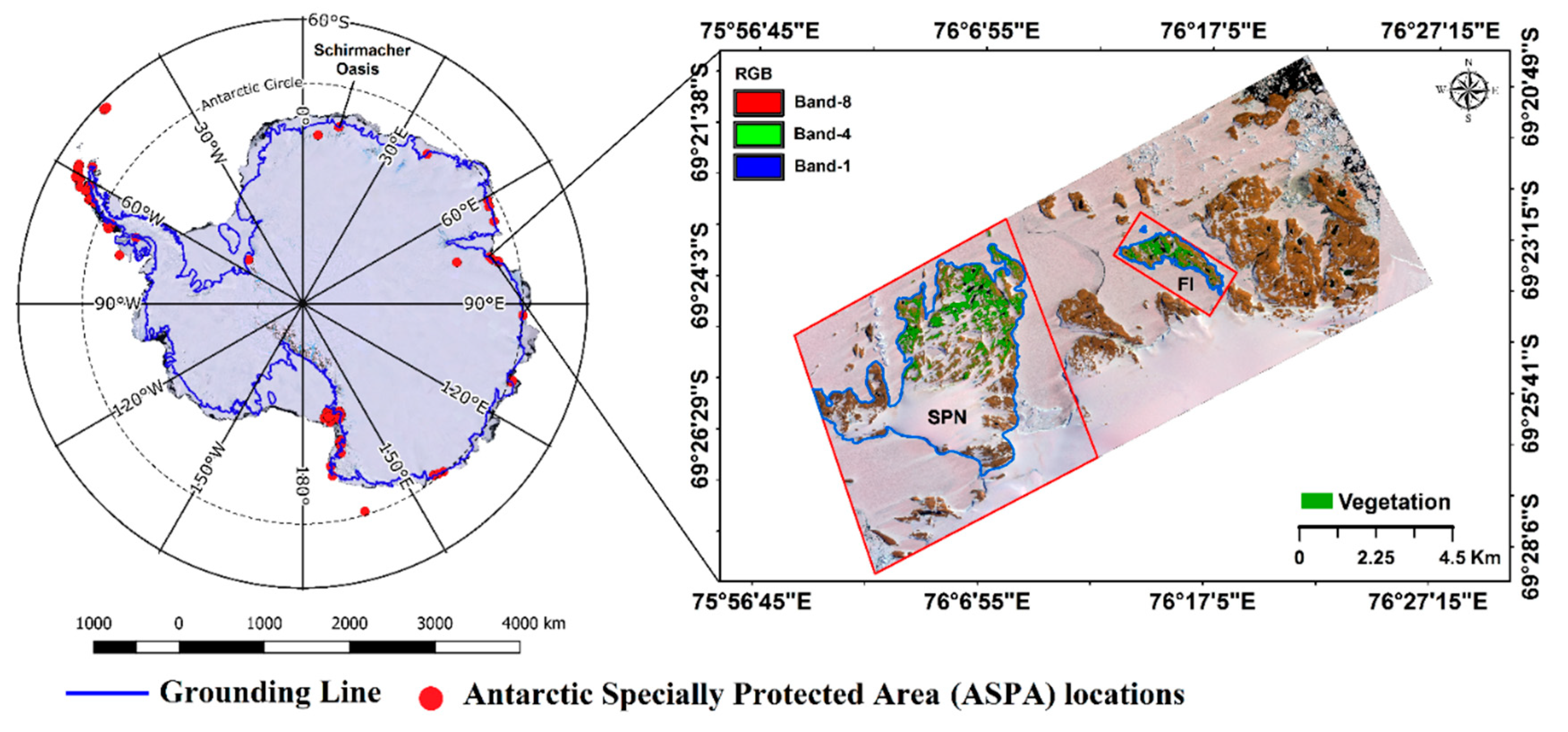
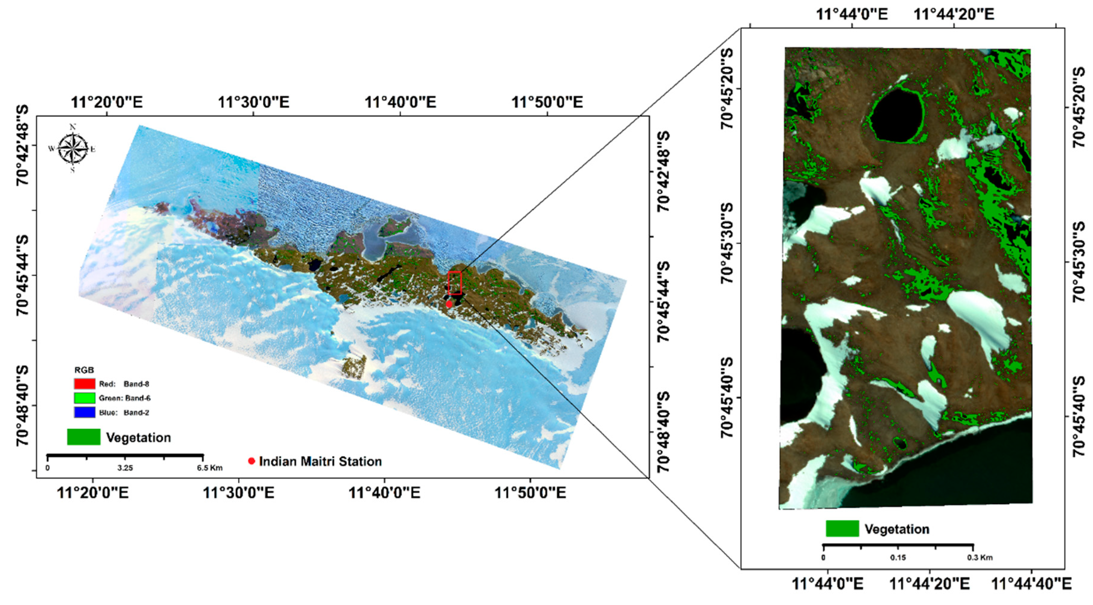
2.1. Study Area

The Larsemann Hills region includes (Figure 1) various land cover features (snow, ice, rocks, lakes, permafrost, etc.) within typically mountainous terrain, and ranges from 5 to 700 m above sea level. The Larsemann Hills (69°20′S to 69°30′S; 75°55′E to 76°30′E) consists of a series of low rounded coastal hills along the south-east shore of Prydz Bay, forming an ice-free oasis on the Ingrid Christensen Coast, Princess Elizabeth Land, situated approximately midway between the eastern margin of the Amery ice shelf and the southern margin of the Vestfold Hills. The Larsemann Hills is the second largest (50 km²) of four major ice-free coastal oases (Vestfold Hills, Larsemann Hills, Holme Bay, and Schirmacher Oasis) located along the ~5000 km coastline of East Antarctica [46,47]. A key characteristic of the climate of the Larsemann Hills is the persistent and strong katabatic winds that blow from the north-east in most of the summer months. Short-term daytime air temperatures during the summer months (December-February) frequently reach 4 °C, with occasional brief peaks of up to 10 °C, and the mean monthly temperature is a little above 0 °C. Mean monthly winter temperatures mostly range between −15 °C and −18 °C. The extreme minimum temperature recorded in the region is −40 °C. Precipitation occurs as snow and does not exceed 250 mm water equivalent annually. There are over 150 lakes in the Larsemann Hills, ranging in salinity from freshwater to slightly saline, and ranging from small ponds less than 1 m deep, to larger ice-deepened basins and glacial lakes with an area/depth of 0.1 km²/38 m. Most lakes are fed by snowmelt, and some have inflow and outflow streams that flow constantly during the summer and provide habitat for crustaceans, diatoms, and rotifers [48].

Vegetation communities are spatially extremely fragmented (patchy) and cover only small areas of the study area. The terrestrial biota of the Ingrid Christensen coast is relatively uniform and restricted to bryophytes, lichens, terrestrial algae, and contained micro-invertebrates. At the study site in the Larsemann Hills, lichens dominate the rocky, ice-free areas, while moss growth is restricted to the vicinity of meltwater, ponds, lakes, streams, and locations where free water is available during the austral summer (November–March). Most terrestrial life is found inland from the coast. Lichen coverage is considerable on north-eastern Stornes and Law Ridge on Broknes, which lie within Antarctic Specially Managed Area 6 (ASMA-6). The terrestrial macro-flora of the Larsemann Hills region consists of at least 31 lichen, seven moss and one liverwort species [48]. Comprehensive systematic studies have not been conducted on the terrestrial and lacustrine algae and cyanobacteria. Additionally, in many regions of seasonal snowmelt, extensive blackened areas can be observed on the soil/substrate surface, indicating the presence of cyanobacteria and microscopic algae. Larger vegetation patches (>200 m²) occur in sheltered sites on the larger islands, associated with Adélie penguin moulting sites, and on nunataks in the south-west of the region. The availability of shelter from the wind and associated abrasion (snow, sand), and the local topographic features play significant roles in determining the distribution and abundance of the cryptogamic flora. In scattered moister sites, small vegetation patches (~1–30 m²) also occur.

2.2. Geospatial Data

A list of satellite and ground reference datasets and their usage is given in

Table 1. A list of satellite and ground truth datasets and their usage status in the present study for effective vegetation mapping. The potential usage of these datasets includes vegetation mapping (VM), visual interpretation and supplementing digitization (VSD), manual digitization (MD), digitization error analysis (DEA), shadow detection and removal (SDR). The notation ✓(✗) denotes used (not used) in this study.

Dataset Details	Source of Datasets	Temporal Range (DD/MM/YY)	Utilization in the Present Study
			VM	VSD	MD	DEA	SDR
WorldView-2 multispectral (2m) and PAN (0.5 m)	DigitalGlobe	09/02/2011	✗	✓	✗	✗	✗
WorldView-2 GS-sharpened image (0.5m)	Processed	09/02/2011	✓	✓	✓	✓	✓
Google Earth Images	Google	31/12/1999, 24/02/2006, 03/03/2006, 04/01/2011	✗	✓	✗	✗	✓
Larsemann Hills, ASMA map series	AADC	Produced in 2013-14	✗	✓	✗	✗	✓
Land cover map (1:2500)	SOI during Indian Antarctic Expedition	2007–2008 (Sep–Mar)	✗	✓	✗	✗	✓
Aerial Photographs	InSEA	2010–2012 (Sep–Mar)	✗	✓	✗	✗	✗
DGPS surveying	InSEA	2008–2011 (Sep–Mar)	✗	✓	✓	✓	✗
DEM	Jawak and Luis [49]	2003–2011	✗	✓	✗	✗	✓

.

2.2.1. Satellite Data

We employed radiometrically corrected, georeferenced, ortho-rectified, 16-bit standard level 2 (LV2A) WV-2 data (DigitalGlobe, Inc., CO, USA), acquired on 9 February 2011, at an off-nadir angle of 14.06° over the Larsemann Hills. The projection and datum of all images were geo-registered with UTM zone 43S and WGS 1984, respectively. The WV-2 image covers an area of 100 km². The period of satellite data acquisition corresponds to the peak of the austral summer (January-February) in Antarctica, when maximum solar radiation reaches the surface on clear days and causes melting of snow and ice. WV-2 offers eight multispectral bands (2 m spatial resolution) and a panchromatic (PAN) band (0.50 m spatial resolution). A WV-2 multispectral image consists of four traditional bands: Band 2, Blue (450–510 nm); Band 3, Green (510–580 nm); Band 5, Red (630–690 nm); and Band 7, Near-IR1 (NIR-1) (770–895 nm) and four new bands, Band 1, Coastal (400–450 nm); Band 4, Yellow (585–625 nm); Band 6, RedEdge (705–745 nm); and Band 8, Near-IR2 (NIR-2) (860–1040 nm).

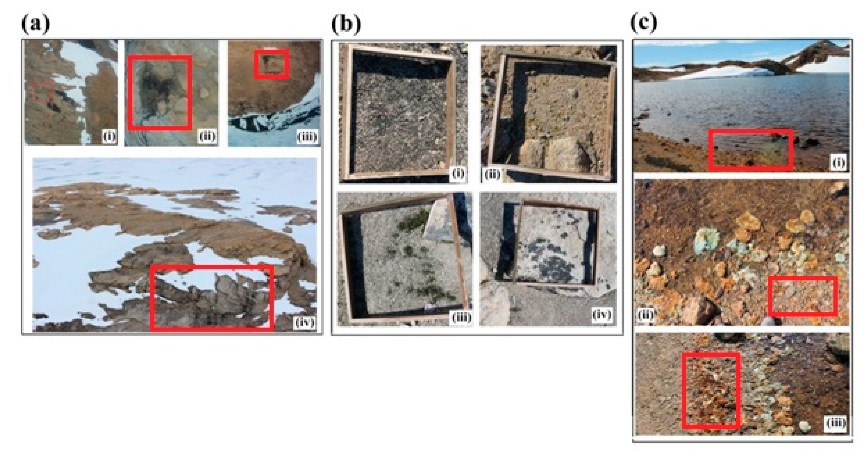
2.2.2. Ground Reference and Supplementary Data

Extensive land cover mapping work has been carried out by the Australian Antarctic Data Centre (AADC) in recent decades (http://www.aad.gov.au/) and by teams from the Indian Scientific Expedition to Antarctica (InSEA) since 2005. An important resource of land-cover data for Larsemann Hills is the AADC “Larsemann Hills Photogrammetric Mapping Project” [50]. The ground reference datasets utilized here to support the semiautomatic extraction of vegetation information were retrieved from the Antarctic Digital Database (ADD), AADC, InSEA, historical Google Earth images, and PAN-sharpened WV-2 images. Historical Google Earth images acquired during the austral summer were used to identify vegetation and to cross-check the spatiotemporal variation of vegetation cover in the study area. The high spatial resolution of WV-2 data facilitates extraction of vegetation patches manually from the PAN-sharpened images. In the case of manual delineation of land cover features in the cryospheric environment, PAN imagery is useful after fusion with the multispectral bands [51]. For this purpose, a fusion of PAN and multispectral bands was carried out using the Gram–Schmidt (GS) PAN-sharpening process. A geo-database consisting of vegetation in the Larsemann Hills region was generated by manual digitization. PAN-sharpened images (0.5 m resolution) were visualized in ArcGIS 10 at several scales using various band combinations of WV-2, viz., 7-4-2, 8-7-2, 6-3-2, 5-3-2, and 7-3-2. However, we could easily recognize the pattern, texture, shape, and size (dimensions) of vegetation, along with better visualization and discrimination of vegetation against background features, using 8 (NIR-2)-5 (Red)-1 (Coastal) band combinations and 1:100 scale. Each digitized polygon was then edited to eliminate digitization errors. Quality control involved cross-checking the selected vegetation polygon boundaries against ground truth data to ensure accurate and consistent interpretation and digitization. Then, the positional accuracy of the digitized vegetation database was calculated using an independent source of 10 accurate differential global positioning system (DGPS) point locations [52,53]. The RMSE of digitization yielded ~47 cm (less than 1 pixel) when compared with the DGPS source. The manually digitized vegetation map (Figure 2) was extensively surveyed, and the features were validated using DGPS ground reference data obtained from field campaigns, existing ADD/AADC maps, ancillary datasets, and multitemporal Google Earth images.

Extensive field surveys were carried out using a Leica Viva DGPS surveying unit in the real-time kinematic mode to delineate and measure areas of vegetated patches during Indian Scientific Expeditions to Antarctica in the austral summer seasons of 2011–2015. Several areas were selected for the measurement of vegetation patches, documenting their shapes, total areas, and spatial extents (boundary). Vegetation communities in the Larsemann hills are mixed, and therefore we did not target only one type of vegetation. There are varying sizes of lichen patches across the study region which were easily visible from reconnaissance survey conducted using a helicopter. Also, to deal with the fragmented nature of these patches, as described by Fretwell et al. [19], we selected larger patches with more than 80 % vegetation cover. This decision was made visually in the field. We collected spatial extent data for vegetation patches from 35 locations (400 m × 400 m; see Supplementary Table S1 and Supplementary Figure S1). A total of 318 vegetated locations were examined. In addition, we also recorded the presence of small vegetation patches from 390 locations using 0.5 m × 0.5 m (equal to the resolution of PAN-sharpened WV-2 image) quadrants to ensure inclusion of very small patches of vegetation. The 318 larger vegetated patches were mapped using DGPS by walking along the outer margins of discrete patches formed by vegetation. The total area of vegetated patches surveyed on ground was estimated to be ~0.92 km². The quality of the manually digitized reference vegetation dataset was tested against the extensively ground surveyed and mapped 318 vegetation patches. The RMSE of the manually digitized map was estimated to be ~20 m². In addition, the 390 small vegetation patches were confirmed on the manually digitized reference map. Since field datasets were collected from 2011 to 2015, they were processed to conform to February 2011 images. Careful visual examination was conducted to eliminate those vegetation patches that were not present in the WV-2 imagery because they may have been covered by snow or ice at the time the image was obtained. Additionally, vegetation patches from two specific study locations (Stornes Peninsula and Fisher Island) (Figure 2), mapped during January–February corresponding to the WV-2 image acquisition date (9 February 2011), were considered in the present analysis in order to reduce any errors associated with temporal changes in spatial extent in vegetation. Vegetation data from these two specific locations mapped using DGPS during January–February were overlaid on the WV-2 PAN-sharpened image and checked against the digitized reference database. After a careful visual analysis, a very small number of manually digitized vegetation regions that had higher variations in spatial extent compared with the field data were corrected manually. Finally, only those vegetation regions extracted by manual digitization and validated by the DGPS survey were considered in the present analysis (Figure 2). A geographical information system (GIS)-compatible shapefile of the vegetation class was generated using ArcGIS 10, and the surface area of vegetation for the two study regions was calculated. Assuming that this manual digitization supplemented by ground truthing was accurate, we then evaluated the performance of various feature extraction methods [54]. A map showing manually digitized reference vegetation cover is presented in Figure 1 and Figure 2. Reference vegetated areas over the two islands (Fisher Island and Stornes Peninsula) were estimated to be 644,710 m² and 2,192,915 m², respectively. Examples of various types of vegetation (black and green colored) observed in the study area during field surveying are depicted in Figure 3.

In the present analysis, these two study areas were selected on the basis of the following criteria: (a) accessible for conducting field survey, (b) including the full spectrum of the varying spatial extent of vegetation in these two regions, (c) approximate availability of matching ground truth data with image acquisition period, (d) previous knowledge of existence of extensive vegetation patches within each site. The final reference map showing vegetated areas on Fisher Island and Stornes Peninsula provides the first accurate map of the area as no previous baseline assessment was available. This was made possible by using VHR satellite data, simultaneous visualization of ground truth polygons, supplementary datasets (e.g., aerial photographs), and ease of identification of vegetated areas based on previous knowledge of the area gained from three field campaigns. Therefore, we consider that the reference map generated in this study is the most accurate map available for the present analysis.

3. Geospatial Analysis

The data processing flowchart is shown in Figure 4, consisting of three stages: (a) data pre-processing, (b) feature extraction, and (c) quantitative evaluation of accuracy.

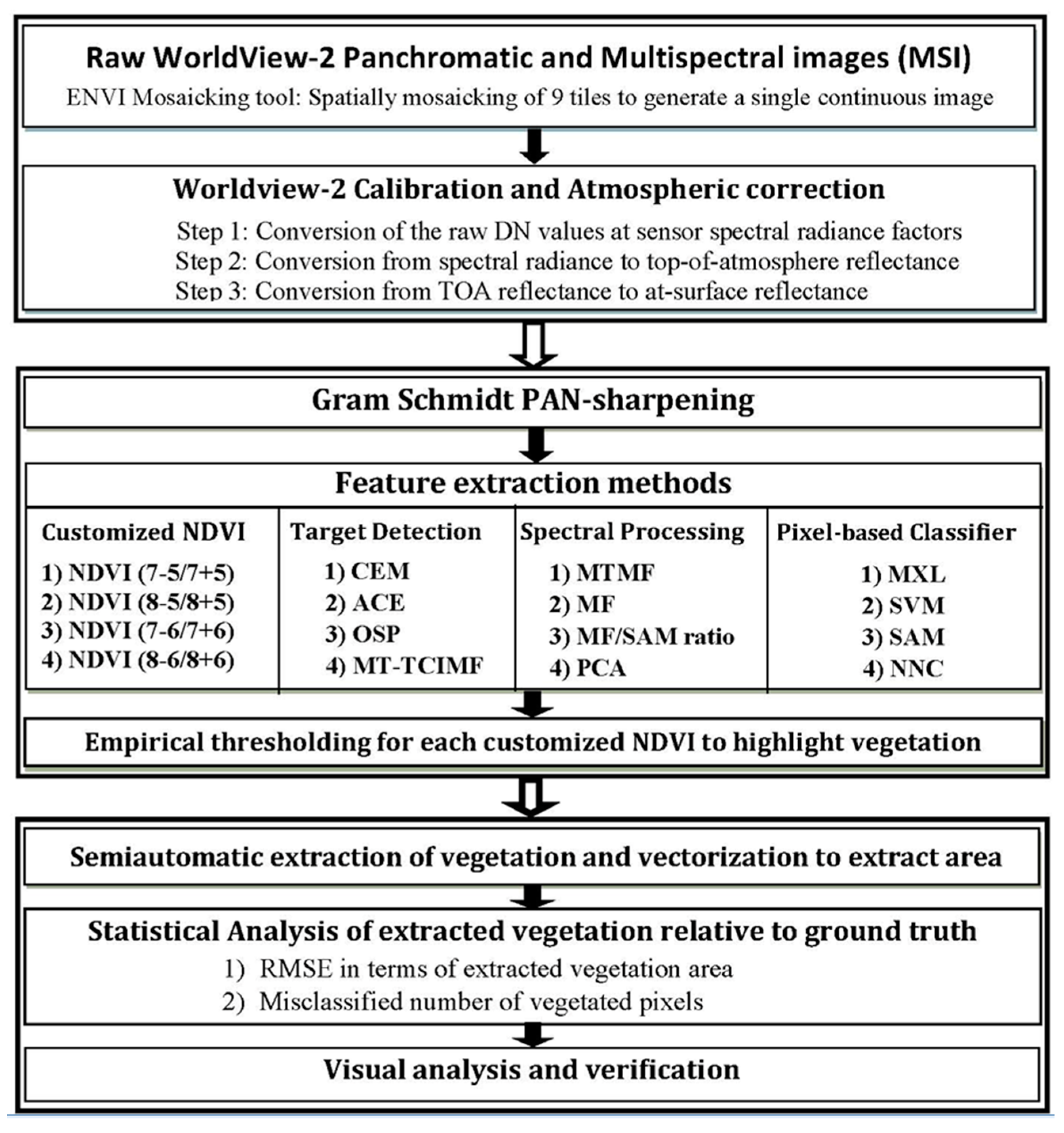
3.1. Data Pre-Processing

The nine WorldView-2 tiles were mosaicked to generate a single continuous image using Environment for Visualizing Images (ENVI) software (version 5; Harris Geospatial Solutions, Boulder, CO, USA). The imagery was radiometrically corrected for internal sensor geometry, optical distortions, scan distortions, line-rate variations, and band registration by data provider [55,56]. The digital numbers (DN) were converted to at-sensor radiance using spectral transmission of the telescope, the spectral quantum efficiency of the detectors, and other calibration parameters provided in the metadata file by using ENVI 5. The at-sensor radiance was corrected for atmospheric influence by applying calibration procedures [57]. The resulting top-of-atmosphere (TOA) reflectance images were converted to at-surface reflectance, using ATmospheric and Topographic CORrection version 3 (ATCOR-3 algorithm) [58] and by using a digital elevation model (DEM) constructed for the Larsemann Hills [49]. This DEM was derived by the synergistic merging of ground-based global positioning system (GPS) measurements, satellite-derived laser altimetry (GLAS/ICESat), and Radarsat Antarctic Mapping Project (RAMP)-based point elevation dataset. Topographic corrections were necessary as the Larsemann Hills region is characterized by rugged mountainous terrain as mentioned in Section 2.1. Model parameters used for ATCOR-3 processing are summarized in Supplementary Table S2. Finally, we synthesized an image at 0.50 m resolution, by PAN-sharpening the multiband image using the Gram–Schmidt (GS) method, which has been shown to be comparatively superior and consistent for sharpening WV-2 data [55]. PAN-sharpening injects spatial detail into the spectral pixels, however, the spectral information in the PAN-sharpened image is slightly distorted. This can cause errors in mapping accuracies. However, in the present context, PAN-sharpening was necessary as we observed vegetation patches of very small sizes (0.25 m²) compared to the 2 m multispectral band pixels. Therefore, it may be desirable to perform PAN-sharpening prior to vegetation index (VI) calculations, particularly for monitoring small vegetation patches [59]. Therefore, we used the GS-sharpening method which causes less spectral distortion. The effectiveness of this sharpening method and subsequent usage of spectral indices derived from GS-sharpened images has been demonstrated in polar regions for mapping lakes and land cover features in Antarctica [3,55,60]. In particular, Jawak and Luis [55] successfully used spectral indices to map land cover features using GS-sharpened WV-2 data in the Larsemann Hills (present study area). Another supporting study on VIs using PAN-sharpened images has been published by Johnson [59], who evaluated the effects of image PAN-sharpening on VIs and found that PAN-sharpening was able to downscale single-date and multi-temporal Landsat 8 VI data without introducing significant distortions in VI values.

3.2. Feature Identification and Mapping

This procedure consisted of four semi-automatic feature extraction approaches: (a) customized NDVI, (b) spectral processing or matching, (c) target detection, and (d) pixel-wise supervised classification. All satellite data were processed by procedures developed using ENVI 5 software.

3.2.1. Customized Normalized Difference Vegetation Index (NDVI) Approach

Numerous mathematical combinations of various spectral bands have been devised for the development of new VIs [61,62,63,64,65,66,67,68,69,70]. NDVI is typically calculated using reflectance values in the red and NIR bands and represented by (NIR−Red)/(NIR+Red). Recently, several normalized difference indices have been developed using WV-2 images, including the normalized difference bare soil index (NDBSI) using blue and coastal blue [71], normalized difference water index (NDWI) using blue/coastal/green and NIR-2 [72], forest and crop index (FCI) from RedEdge and NIR-1, normalized difference soil index (NDSI) from green and yellow bands, and non-homogeneous feature difference (NHFD) from RedEdge and coastal bands [73]. There is a plethora of VIs proposed in the literature to map vegetation in different environments. The majority of these VIs were designed for vegetation canopies such as forests, croplands, and grasslands, and most have rarely or never been tested in complex environment of Antarctica’s sparse vegetation. Vegetation in the Larsemann Hills occurs in a variety of patches which are characterized by different features (size, shape, morphology), varying amount of stress (due to limited sunlight, water, and availability of nutrients), changing weather conditions (e.g., snowfall), various coloration (green, black, brown, yellow), different forms (wet and dry), species (bryophytes, lichens, mosses, algae, cyanobacteria), different rates of growth, and varying amounts of pigments (e.g., chlorophyll and carotenoids). With such a mixed vegetation structure, it is almost impossible to identify such a mixed vegetation by simply using spectral response from one type of NDVI. This is because spectral responses of cryospheric vegetation types are related to various factors (e.g., dry or wet soil background). Furthermore, single model NDVIs may exhibit certain randomness in results. Therefore, in addition to the traditional NIR-red NDVIs, we used RedEdge [70] versions of NDVI using 2 NIR bands of WV-2, which have higher sensitivity to chlorophyll content and plant stress compared to the traditional red band.

Our customized NDVIs were developed using NIR-1 and NIR-2 and Red and RedEdge spectral bands of WV-2 for the effective extraction of cryospheric vegetation, in comparison to supervised feature extraction methods. The eight spectral bands of the WV-2 satellite images were ranked in terms of mutual information (MI)–the minimum-redundancy-maximum-relevance (mRMR) criterion [74] coupled with a robust repetitive visual analysis of spectral profiles of vegetation class, and the two bands with minimum and maximum mRMR score were used to generate NDVI. This method distinguishes the most useful spectral bands based on the fact that vegetation strongly absorbs solar radiation in the visible spectrum and reflects in NIR (Supplementary Figure S2). Spectral profile indicated that the reflectance ranged from 35–65% for vegetation, while that for yellow, green, red, and RedEdge bands were comparable for most of the vegetation profiles. The minimum reflectance rendered by these four bands can be used to identify the vegetation on these images. A comparison of spectral curves indicates that the Red and NIR bands have the most spectral utility for vegetation discrimination. So, in this work, four customized VIs were recreated to incorporate new WV-2 bands and to provide a wider context to the analysis (

Table 2. Customized normalized difference vegetation index (NDVI) devised as an effective semi-automatic extraction tool for vegetation mapping application.

NDVI	NDVI Model	Formula	Threshold Range
NDVI-1	NDVI(7-5/7+5)	$\frac{\mathrm{NIR}1-\mathrm{Red}}{\mathrm{NIR}1+\mathrm{Red}}$	0.53−0.65
NDVI-2	NDVI(8-5/8+5)	$\frac{\mathrm{NIR}2-\mathrm{Red}}{\mathrm{NIR}2+\mathrm{Red}}$	0.57−0.62
NDVI-3	NDVI(7-6/7+6)	$\frac{\mathrm{NIR}1-\mathrm{RedEdge}}{\mathrm{NIR}1+\mathrm{RedEdge}}$	0.54−0.63
NDVI-4	NDVI(8-6/8+6)	$\frac{\mathrm{NIR}2-\mathrm{RedEdge}}{\mathrm{NIR}2+\mathrm{RedEdge}}$	0.55−0.66

). After customization of NDVI, output images were generated for each NDVI model. The difference between the response values in the NDVI determines where the vegetation patches are located on the scene. Once these areas were identified from the NDVI images, the optimal threshold ranges (Table 2) were set to capture only vegetated regions of classification. After the threshold ranges were set, the vegetated regions were grouped into one class. Following literature on spectral indices [19,72], we used a manual thresholding method to map vegetated areas from NDVI images. A detailed description of the thresholding process is given in Supplementary Material 1.

Vegetation was considered as a single broad class in the present study instead of classifying the entire vegetation exhibiting various colors, types and texture. This decision was based on multiple aspects of the study. First, all the vegetation forms are sporadically distributed in the entire study area without any specific boundary and, when mapping vegetated patches in the field, all types of vegetation were included independent of color, species or type. Spectral responses of such a complex vegetation will be mixed and, to separate out such vegetation areas using satellite reflectance values would potentially need broad ground truthing to collect ground spectral response of all vegetation types and eventually matching the ground spectra with satellite-based reflectance. Such an exercise would also potentially need laboratory spectral analysis which would include collection of various types of vegetation samples and analyzing spectra with artificial illumination, because of the infrequency of good weather days suitable for such experiments in the field. Second, as these different types of vegetation would exhibit different patterns of NDVI values, we have taken care to avoid errors or discrepancies in NDVI threshold range. The threshold range (Tmin-Tmax) was empirically defined by repeat observation or manually scrutinizing the most obvious medium, sparse, and dense vegetation patches consisting of various amounts of different types of vegetation forms on the NDVI images, as confirmed by ground-truth data. By doing this, we used a range of values (Tmin-Tmax) showing vegetation as one class rather than introducing unnecessary complexity or source of inaccuracy.

After executing customized NDVI, we processed the WV-2 image to map vegetation using spectral processing, target detection, and pixel-wise feature extraction methods as listed in

Table 3. Target detection, spectral processing and pixel-wise supervised classification approaches and their relevant methods along with their acronyms used in present analysis.

Category/Approach	Acronym	Method Name
Target detection	MT-TCIMF	Mixture Tuned Target-Constrained Interference-Minimized Filter
	CEM	Constrained Energy Minimization
	ACE	Adaptive Coherence Estimator
	OSP	Orthogonal Subspace Projection
Spectral processing	MTMF	Mixture Tuned Matched Filtering
	MF	Matched Filtering
	MF/SAM	Matched Filtering/Spectral Angle Mapper Ratio
	PCA	Principle Component Analysis
Pixel-wise supervised	MXL	Maximum Likelihood Classifier
classification	SVM	Support Vector Machine
	NNC	Neural Net Classifier
	SAM	Spectral Angle Mapper

.

3.2.2. Spectral Processing or Matching–Based Extraction Approach

Spectral matching methods extract the target features that are depicted in multispectral imagery based on the target feature’s spectral characteristics. The supervised workflows require an initial approximation in terms of regions of interest (ROIs) as reference spectra or seed points that include representative pixels of the desired target class. Spectral matching algorithms determine the spectral similarity or matching between input satellite imagery and reference seed points to create an output product in which pixels with similar spectral properties are clumped into target and non-target classes. The spectral processing or matching-based extraction approach was conducted via Spectral Processing Exploitation and Analysis Resource (SPEAR) workflow tools, terrain categorization (TERCAT) and mapping methods (ENVI 5), which streamline spectral processing methods (MF, MTMF, MF/SAM ratio, and PCA) for mapping vegetated areas using WV-2 PAN-sharpened data [72]. Vegetation showed a wide range of shades of color, ranging from grey/black dried powdered instances of moribund dormant/dead moss on rocky surfaces to greenish (open-leaved form) or yellowish/reddish (denser and closed packed) patches on hilly slopes, along with wet brownish leafy patches near water bodies. Because of this difference in spectral information, unsupervised classification methods were not used for automated vegetation mapping. Since one of our objectives was to extract vegetation semi-automatically, we processed the image using supervised workflows based on the knowledge of vegetation locations within the landscape.

MF is used to detect and map the abundances of target class (here vegetation) by using a partial unmixing technique, which maximizes the spectral response of the known spectra (vegetation) and suppresses the spectral response of the non-target (if defined) and unknown targets in image background by matching the target’s spectral signature. It does not necessarily require non-target spectral signature for mapping the target feature. In the present study, we used the ENVI 5 implementation (via Mapping Methods workflow) to map vegetation using input ROIs and a background (non-target) threshold of 0.7 (0.5 to 1 defines the entire image).

MTMF is a modified version of MF which couples with Minimum Noise Fraction (MNF) to add an infeasibility image to the results. We used the ENVI 5 implementation to execute MTMF via Mapping Method workflow to generate an MF (background threshold 0.7) score image and infeasibility score image. Finally, both images were thresholded using a higher MF score (0.8, where 1 is maximum) and low infeasibility score (0.1 where 1 is maximum).

SAM is a physically-based spectral classification that uses an n-D angle (here, 8-D space for WV-2 bands) represented by shape of spectra to match pixels to reference target spectra (here, vegetation). Here, we used the ENVI 5 implementation using input ROIs and setting the default threshold value of 0.03 radians to the rule image generated before the final classification of vegetation. After deriving MF and SAM, rule images were divided to set the threshold for MF/SAM classification to suppress false positives and enhance true positives for vegetation class. We implemented the SPEAR Spectral Analogues Tool of ENVI 5 to execute MF/SAM ratio by setting a threshold of 0.13 to the rule image.

PCA is widely used for dimensionality reduction to effectively process high spectral-dimension data. In this study, variance-covariance based PCA was applied to eight spectral bands of WV-2 to obtain principal components (PCs). The eigen values and variance values computed for all the eight PCs were ranging from 30 to 1700 and 0.1 to 90, respectively. First four PCs were chosen for further classification as these four contain more than 95% of total information. ROIs were selected from these four PCs and are subsequently utilized for classification using a typical supervised classification workflow using Mahalanobis Distance in ENVI 5 implementation.

3.2.3. Target Detection Approach

Target detection algorithms work on the principle of extracting target features based on a spectral characteristic of initial training spectral signatures of target features and suppressing the background noise using spectral signatures of non-target features. The initial approximations or spectral signatures for supervised workflows are provided in terms of target ROIs and non-target ROIs. Target detection workflow introduced by Jin et al. [75] that couples a Minimum Noise Fraction (MNF) transform were executed using ENVI 5 Target detection wizard to perform supervised image processing tasks in workflows (CEM, ACE, OSP, and MT-TCIMF) to extract vegetation. Additionally, for MT-TCIMF, the MNF-transformed image fuses the mixture-tuned method with the TCIMF method. Hence, the MNF was used to resolve the intrinsic spectral dimensionality of the WV-2 image to support subsequent processing. The MNF transformation was used to (a) extract target features and/or reduce dimensions for ACE, CEM, and OSP methods, and (b) generate isotropic variance noise, which was used to compute infeasibility value for the mixture tuned method (MT-TCIMF) [72]. By adding an additional infeasibility band, mixture tuned techniques improve the detection results by reducing the number of false spectral signals.

CEM uses a finite impulse response filter to allow the target class (vegetation) pixels while suppressing response from background spectra (non-target). ACE used in the present study is derived from the Generalized Likelihood Ratio (GLR) approach, which makes ACE almost constant to relative scaling of input ROIs. OSP first defines an orthogonal subspace projector to remove the spectral response of background (non-target), followed by application of MF to match the target spectra. MT-TCIMF is the combination of the mixture tuned technique and TCIMF target detector. It uses an MNF transform to execute TCIMF and adds an infeasibility image to the results. The MT-TCIMF produces two images: (1) a rule image of TCIMF scores, and (2) an infeasibility image. All the target detection methods were executed using a subspace background threshold (0.5) which resulted in rule images at the final stage, which we thresholded as: CEM (0.7, range 0.5–1), ACE (0.6, range 0.5–1), OSP (0.7, range 0.5–1), and MT-TCIMF (TCIMF 0.6, infeasibility 0.2).

3.2.4. Pixel-Wise Supervised Classification Approach

We used four distinct pixel-based classification methods to classify the WV-2 PAN-sharpened data: MXL, SVM, NNC, and SAM. The robustness of these classifiers in mapping land-cover features using VHR imagery has been demonstrated elsewhere [76]. The GS-sharpened WV-2 image was classified into target (vegetation) and non-target (melt water, snow/ice, landmass, lakes), so as to reduce the time required to produce the final vegetation map.

MXL assumes that the statistics for each class (vegetated and non-vegetated) in each spectral band of WV-2 are normally distributed and estimates the probability of a pixel to be classified to a particular target class; pixels are assigned to the class of highest probability. We used the ENVI 5 classification tool to execute the MXL using input ROIs and a probability threshold 0.4 (pixels below this threshold were unclassified). SVM is a supervised classification method derived from statistical learning theory to classify each pixel of the image data. The supervised classification tool of ENVI 5 was used to implement radial basis function kernel-based SVM by providing input ROIs and training set parameter values [Gamma in kernel function (γ): 0.30, penalty parameter (C): 200, pyramid level: 0: classification probability threshold: 0.3]. NNC uses standard backpropagation for supervised learning. In the present study, the most widely used multilayered feed-forward/multilayer perceptron (MLP) NN model was implemented using the ENVI 5 classification tool by providing input ROIs and setting necessary parameters [Activation function: logistic, training threshold contribution: 0.7, training rate: 0.1, training momentum, 0.8, training root mean square exit criteria: 0.04, number of hidden layers: 1, number of training iterations: 2000].

The vegetation classification using target detection, spectral processing, and pixel-wise supervised classification methods was based on the prior knowledge of spectral response of the vegetation in the study area. Even though the reference map was generated using ground-truthing and digitization, the entire separated vegetated areas were not used for the training of classification, but the spectral response from a proportion of the known vegetated areas were used for training and thresholding various methods.

Feature extraction methods described in this section are based on different underlying principles. Hence, to compare these methods objectively, we kept the input ROIs (training samples) constant for all methods. For the sharpened image, we selected ROIs (~1000 pixels) for non-target and target (vegetation) classes, as training pixels using spectral signature observations. The training datasets were randomly selected based on manual interpretation of the PAN-sharpened image, ground truth, and using VHR historical images for different dates from Google Earth. Individual reference spectra (end members) for the vegetation class were generated as ROIs over spatially and spectrally homogeneous targets on PAN-sharpened images. ROIs were selected by carefully considering the vegetation unit size identified and sampled on the image, which minimized the mixed pixels. Finally, feature extraction methods were executed using common input ROIs for all three techniques, i.e., spectral processing, target detection, and pixel-wise supervised classification. In the final stage, we note that the changes in threshold values used for different methods used in the present study would affect the final result of vegetation estimate. However, to ensure a relatively, if not completely, unbiased accuracy analysis, the thresholding process was conducted semiautomatically on a trial-error basis. Rule images generated before the final classification using the 12 methods were observed carefully and threshold values were set based on the visual observations of 10 most obvious vegetated patches. Finally, after classifying the image into target class, i.e., vegetation, using the 16 feature extraction methods based on customized NDVI, spectral processing, pixel-wise supervised classification, and target detection approaches, the semiautomatically extracted vegetated regions were vectorized to calculate the vegetation area. We compared these calculated vegetated areas with that of manually digitized reference vegetated area and evaluated statistical significance of each feature extraction method based on the accuracy assessment. Finally, we also evaluated the performance of these methods with regards to computational processing time.

3.3. Accuracy Assessment

The results of the extraction methods were assessed using visual analysis and statistical approaches. To test the contribution of varying land cover features in causing misclassification in vegetation mapping, we conducted repeat visual observations of 16 output vegetation maps derived using semiautomated methods against the PAN-sharpened imagery and/or manually digitized vegetation map supplemented by ground truth data. The visual observations were made by three independent observers with field experience in the Antarctic environment. Statistical analysis was conducted on vectorized maps by comparing vegetated areas mapped from satellite imagery using semiautomatic methods against (a) the manually digitized reference vegetation map for the study region [54,72] and (b) the ground truth data collected using DGPS. A pre-digitized geo-database of vegetation covering areas of Fisher Island and the Stornes Peninsula was utilized as a reference for assessing the accuracy of the semiautomatic extraction methods. As the spatial resolution of the WV-2 PAN-sharpened image was 0.5 m, each misclassified pixel or false signal can introduce a bias of 0.25 m² in the semiautomatically extracted vegetation area. Bias (%) for extracted vegetation is defined as: (A_reference − A_measured) × 100, where A_reference is the manually digitized vegetation area or ground truth reference data, and A_measured is the vegetation area calculated by semiautomatic extraction method. A positive (negative) bias indicates an average amount of underestimation (overestimation). Root mean square error (RMSE), a consistent and statistically significant indicator of accuracy, was used to quantify the uncertainty in extracted vegetation area using the four approaches. Mathematically, $\mathrm{RMSE}=\sqrt{\frac{1}{\mathrm{n}}{\sum }_{\mathrm{i}=1}^{\mathrm{n}}{\left(VA{\mathrm{r}}_{\mathrm{i}}-VA{\mathrm{m}}_{\mathrm{i}}\right)}^2,}$ where VAm_i is the i^th original vegetated area value estimated using the individual semiautomatic extraction method, VAr_i is the corresponding vegetated area derived using the reference (manual digitization and/or ground truth), and n is the number of methods in one approach.

4. Results

The performance of the customized NDVI-based semi-automatic extraction approach was compared with the supervised semi-automatic feature extraction approach by computing bias and RMSE values of the extracted vegetation areas. The performance of the 16 feature extraction algorithms (grouped as four approaches) was also compared in terms of their ability to extract vegetation. Visual analysis of extracted vegetated maps against reference vegetation maps are depicted in Figure 5 and Supplementary Figures S3–S6.

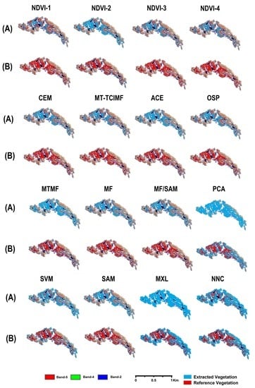
4.1. Performance of the Customized Normalized Difference Vegetation Index (NDVI) Approach

In terms of accuracy assessment based on manually digitized reference vegetation data (supplemented with ground truth data), the NDVI-2 (bias: Fisher Island = 14,950.85 m², Stornes Peninsula = 167,790.95 m²) combination yielded superior results, while NDVI-1 (bias: Fisher Island = 16,107.10 m², Stornes Peninsula = 311,774.22 m²) performing the worst, when compared to the remaining two combinations (

Table 4. Quantitative evaluation of various feature extraction methods for extracting vegetation from Fisher Island (FI), Stornes Peninsula (SPN), and cross-validation with Schirmacher Oasis (SO) in terms of bias in extracted vegetated area (m²). The lowest (italics) and highest (bold) values in each local column are highlighted. The column-wise average values are in bold and underlined. Methods that cause overall overestimation (negative bias values) of vegetation are highlighted with the grey background colour. Global outliers (with respect to all 16 methods) are highlighted with ^ marks while local outliers (with respect to the four methods in the approach) are highlighted with * marks.

		Bias in Extracted Vegetated Area (m2)
		Experiment				Cross-Validation
Approach	Reference	FI	SPN	Total	Average	SO
Customized NDVI Approach
NDVI-1	Present work	16107.10	311774.20	327881.30	163940.70	167060.08
NDVI-2	Present work	14950.85	167791.00	182741.80	91370.90	114117.37
NDVI-3	Present work	15518.06	284756.50	300274.60	150137.30	161572.11
NDVI-4	Present work	15093.41	170286.70	185380.10	92690.06	117345.58
	Average	15417.36	233652.10	249069.50	124534.70	140023.78
	RMSE	15423.91	242611.20	257600.10	128800.10	142133.19
Target Detection Approach
MT-TCIMF	[75]	15349.75	259172.20	274522.00	137261.00	153017.34
OSP	[77]	15727.75	290478.20	306206.00	153103.00	164800.33
ACE	[78]	−15470.50	−279690.00 *	−2951610.00 *	−147580.00 *	−160926.47
CEM	[79]	16382.61	437713.50	454096.10	227048.00	225813.57
	Average	7997.40	176918.40	184915.80	92457.90	95676.19
	RMSE	15737.72	324564.20	340017.50	170008.70	178509.49
Spectral Processing Approach
MTMF	[80]	−14083.00	−84882.90	−98965.90	−49483.00	−80866.76
MF/SAM	[81]	14329.33	145633.00	159962.30	79981.15	106046.83
MF	[82]	14405.00	169909.60	184314.60	92157.32	115085.83
PCA	[75]	−146687.00 ^*	−744066.00	−890752.00	−445376.00	−473579.00
	Average	−33008.90	−128351.00	−161360.00	−80680.20	−83328.27
	RMSE	74377.72	390805.90	464433.50	232216.70	252639.65
Pixel-wise Supervised Classification Approach
SVM	[83]	−18217.40	−502521.00	−520739.00	−260369.00	−240017.71
SAM	[84]	15989.08	361368.90 *	377358.00 *	188679.00	218388.68
NNC	[85]	−95117.40 ^	−518722.00	−613839.00	−306920.00	−340737.99
MXL	[86]	−155180.00 ^	−488940.00	−644120.00	−322060.00	−390291.08
	Average	−63131.50	−287204.00	−350335.00	−175168.00	−188164.52
	RMSE	91809.25	472030.20	548921.10	274460.60	305667.96
	Total Average	−18181.40	−1246.14	−19427.50	−9713.77	−8948.21
	Total RMSE	60096.91	367336.30	418025.90	209012.90	228761.44

and

Table 5. Quantitative evaluation of various feature extraction methods for extracting vegetation from Fisher Island (FI), Stornes Peninsula (SPN), and cross-validation with Schirmacher Oasis (SO) in terms of misclassified vegetated pixels (%). The lowest (italics) and highest (bold) values in each local column are highlighted. The column-wise average values are in bold and underlined. Methods that cause overall overestimation of vegetation are highlighted with the grey background colour. Global outliers (with respect to all 16 methods) are highlighted with ^ marks while local outliers (with respect to the four methods in the approach) are highlighted with * marks.

		Misclassified Vegetated Pixels (%)
		Experiment				Cross-Validation
Approach	Reference	FI	SPN	Total	Average	SO
Customized NDVI
NDVI-1	Present work	2.50	14.22	11.55	8.36	10.35
NDVI-2	Present work	2.32	7.65	6.44	4.99	7.07
NDVI-3	Present work	2.41	12.99	10.58	7.70	10.01
NDVI-4	Present work	2.34	7.77	6.53	5.05	7.27
	Average	2.39	10.65	8.78	6.52	8.68
	RMSE	2.39	11.06	9.08	6.70	8.81
Target Detection Approach
MT-TCIMF	[75]	2.38	11.82	9.67	7.10	9.48
OSP	[77]	2.44	13.25	10.79	7.84	10.21
ACE	[78]	2.40	12.75	10.40	7.58	9.97
CEM	[79]	2.54	19.96 *	16.00 *	11.25 *	13.99
	Average	2.44	14.44	11.72	8.44	10.91
	RMSE	2.44	14.80	11.98	8.60	11.06
Spectral Processing Approach
MTMF	[80]	2.18	3.87	3.49	3.03	5.01
MF/SAM	[81]	2.22	6.64	5.64	4.43	6.57
MF	[82]	2.23	7.75	6.50	4.99	7.13
PCA	[75]	22.75 *^	33.93 *	31.39 *	28.34 *^	29.34
	Average	7.35	13.05	11.75	10.20	12.01
	RMSE	11.54	17.82	16.37	14.64	15.65
Pixel-wise Supervised Classification Approach
SVM	[83]	2.83	22.92	18.35	12.87	14.87
SAM	[84]	2.48	16.48 *	13.30	9.48	13.53
NNC	[85]	14.75 ^	23.65	21.63	19.20	21.11
MXL	[86]	24.07 ^	22.30	22.70	23.18^	24.18
	Average	11.03	21.34	19.00	16.18	18.42
	RMSE	14.24	21.53	19.34	17.04	18.94
	Total Average	5.80	14.87	12.81	10.34	12.51
	Total RMSE	9.32	16.75	14.73	12.49	14.17

).

However, the differences in bias for NDVI-3 (Fisher Island = 15,518.06 m², Stornes Peninsula = 284,756.52 m²) and NDVI-1 were comparable in the group of four NDVIs. Similarly, the performance of NDVI-4 (bias: Fisher Island = 15,093.41 m², Stornes Peninsula = 170,286.70 m²) and NDVI-2 were similar. NDVI-2 (total misclassified pixels = 6.44 ± 1.34%) and NDVI-4 (total misclassified pixels = 6.53 ± 1.34%) yielded ~2 times better results than NDVI-1 (total misclassified pixels = 11.55 ± 1.34%) and NDVI-3 (total misclassified pixels = 10.58 ± 1.34%) (Table 4 and Table 5).

In general, all the NDVI methods underestimated vegetation area by between 6.44 ± 1.34 and 11.55 ± 1.34% and yielded misclassified (underestimated) pixels significantly higher for Stornes Peninsula (10.65 ± 1.71%, on average) as compared to Fisher Island (2.39 ± 0.04%, on average). On average, the NDVI methods identified total vegetation area of 2,588,556.48 ± 37,957.17 m² from Fisher Island and Stornes Peninsula. The customized NDVI approach was significantly superior to the pre-existing pixel-wise supervised classification and comparable to spectral processing and target detection methods. We note that NDVI-3 and NDVI-4, designed using RedEdge band, produced 17.99 ± 1.34% misclassified pixels relative to manually digitized reference and 1.51 ± 0.04% relative to ground truth vegetation, but produced results similar to NDVI-1 and NDVI-2, which were designed using red band (total misclassified pixels, 17.11 ± 1.34% relative to manually digitized reference and 1.57 ± 0.04% relative to ground truth) (Figure 6 and Figure 7).

We note that NDVI-2 and NDVI-4 (using NIR-2) performed significantly better (12.97 ± 1.34% misclassified pixels relative to manually digitized reference and 1.42 ± 0.04% relative to ground truth) than NDVI-1 and NDVI-3 (using NIR-1) (22.13 ± 1.34% total misclassified pixels relative to manually digitized reference and 1.66 ± 0.04% relative to ground truth). This implies that the normalization of RedEdge and red bands against NIR-2 yields superior results over normalizing against NIR-1, because the RedEdge band (705–745 nm), being at the top portion of the electromagnetic spectrum, is less affected by atmospheric influence, so it facilitates a better discrimination between healthy and stressed vegetation than NIR-1. The misclassification represented by positive bias (average: Fisher Island = 2.39 ± 0.04%, Stornes Peninsula = 10.65 ± 1.72%) led to overall underestimation of vegetation by all four NDVI methods. In terms of misclassified numbers of pixels, the NDVI approach yielded 35.11 ± 1.34% (average: 8.78 ± 1.34%, RMSE 9.08 ± 1.34%) underestimation of vegetated pixels. Overall, the accuracy of the customized NDVI approach exceeded that of the other three approaches.

In terms of accuracy assessment based only on ground truth reference vegetation data (Supplementary Table S3), NDVI-2 was superior in the cohort of four NDVI methods, accurately detecting 88.32 ± 3.59% of small vegetation patches and 88.05 ± 3.09% of medium/large vegetation patches with respect to ground truth data. Overall, the success rate using the NDVI approach for detecting small vegetation patches was 81.30 ± 3.59% relative to ground truth vegetation presence data for small patches. As for mapping larger vegetation patches, the detection success rates of the NDVI approach were 82.08 ± 3.09%, relative to ground truth vegetation. The performance of all four NDVI methods can be ranked in the order: NDVI-2 > NDVI-4 > NDVI-3 > NDVI-1.

4.2. Performance of the Target Detection Approach

Among the four target detection methods applied to the WV-2 images, the MT-TCIMF (bias, Fisher Island = 15,349.75 m², Stornes Peninsula = 259,172.23 m²) outperformed the other methods, while CEM (bias, Fisher Island = 16,382.61 m², Stornes Peninsula = 437,713.45 m²) performed the worst in a given cohort of methods for extracting vegetation (see bias in Table 4 and Table 5). MT-TCIMF, CEM, and OSP all underestimated the vegetation, while ACE produced an overestimation. The overestimation of vegetation caused by ACE was less than the underestimation caused by OSP. Overall, the target detection approach extracted a total vegetation area of 2,652,710.13 ± 164,740.20 m² (average) from Fisher Island and Stornes Peninsula. The underestimation (average: 12.15 ± 1.45%) associated with three target detection methods (MT-TCIMF, OSP, and CEM) outweighed the overestimation of ACE (10.40 ± 1.45%). Overall, the target detection approach gave comparable performance to the accuracy associated with the customized NDVI and spectral processing approach, while its performance in terms of average bias was superior to the pixel-wise supervised classification approach. ACE yielded superior success rates for detecting the presence of 87.59 ± 3.90% of small vegetation patches and 84.96 ± 3.36% of medium/large vegetation patches relative to ground truth data in comparison with the remaining 3 target detection methods in the cohort (Supplementary Table S3). However, ACE also caused an overall overestimation of vegetation. Therefore, there is a trade-off between the higher detection rates and the overall overestimation. The overall performance ranking for all four methods is summarized in Table 4 and Table 5 and Figure 6 and Figure 7 and is MT-TCIMF > ACE > OSP > CEM.

4.3. Performance of the Spectral Processing Approach

The MTMF spectral processing method (bias: Fisher Island = 14,083.00 m², Stornes Peninsula = 84,882.93 m²) produced the best results compared to the other methods trialled. The MF/SAM (bias: Fisher Island = 14,329.33 m², Stornes Peninsula = 145,632.96 m²) ratio method performed better than its individual components, i.e., SAM (bias: Fisher Island = 15,989.08 m², Stornes Peninsula = 361,368.94 m²) and MF (bias: Fisher Island = 14,405.00 m², Stornes Peninsula = 169,909.64 m²), as expected (Table 4 and Table 5). The difference in bias values between MF/SAM (5.64 ± 0.89%) and MF (6.50 ± 0.89%) was comparable to the difference in bias between MF/SAM and SAM (13.30 ± 0.89%), which indicates that the poor performance of MF/SAM may be attributed to the overall poor performance of the SAM component. Overall, the spectral processing approach extracted a total vegetation area of 2,998,986.27 ± 251,436.70 m² from Fisher Island and Stornes Peninsula. MTMF and PCA both overestimated the vegetation, while MF/SAM and MF generated underestimates.

The performance of PCA (–890,752.34 m² total bias and 31.39 ± 0.89% total misclassified pixels) was inferior to all four feature extraction methods. In terms of misclassified pixels, spectral processing gave 34.88% overestimation and 12.14% underestimation of pixels within the total 47.01 ± 6.58%. In general, the performance of spectral processing in terms of bias was superior to that of pixel-wise supervised classification and target detection, and comparable to NDVI, although it is also noted that MTMF, MF/SAM, and MF individually performed better than the customized NDVI approach. The overall poor performance of the spectral processing approach (in comparison to target detection) can be attributed to the poor performance of the PCA method. The PCA and MTMF methods outperformed the other two spectral processing methods, with success rates of 95 ± 3.30% and 91 ± 3.30%, respectively, for detecting vegetation patches relative to ground truth data (Supplementary Table S3). However, their higher success rates were accompanied by overestimation. MTMF overestimated by 1022.02 m² (0.40 ± 0.07%), while PCA caused the highest negative bias of 3228.20 m² (1.28 ± 0.07%) relative to ground truth. Based on the statistics (Table 4 and Table 5, Figure 6 and Figure 7), the overall performance for the spectral processing methods is ranked as follows: MTMF > MF/SAM > MF > PCA.

4.4. Performance of the Pixel-Wise Supervised Classification Approach

SAM (bias: Fisher Island = 15,989.08 m², Stornes Peninsula = 361,368.94 m²) performed best, while MXL (bias: Fisher Island = 155,180.26 m², Stornes Peninsula = 488,940.18 m²) performed worst in the group of four practiced pixel-based classification methods (Table 4 and Table 5). However, the differences in total bias for MXL (644,120.44 m²) and NNC (613,839.20 m²) were comparable in any given group. MXL, SVM and NNC overestimated the vegetation, while SAM underestimated it. SAM underestimation contributed less in comparison to the overestimation by SVM, MXL, and NNC for misclassification of the vegetated area (total bias). MXL yielded the most misclassified vegetated pixels. Overall, the pixel-wise supervised classification approach extracted a vegetation area of 3,187,961.01 ± 59,939.42 m² for Fisher Island and Stornes Peninsula. In terms of misclassified numbers of pixels and bias, the pixel-wise supervised classification approach yielded a total of 75.98% (average: 19.00 ± 2.11%) misclassified pixels and was inferior to the other three feature extraction approaches. The accuracy assessment against ground truth data (Supplementary Table S3) revealed that NNC and MXL performed better than the other two pixel-wise supervised classification approaches, with comparable success rates of 88 ± 5.23% (small patches) and 85–87 ± 4.69% (medium/large patches). Again, these higher success rates were associated with an overall overestimation. The SAM results produced the least bias of 2,170.98 m² (0.86 ± 0.09%), while NNC and MXL showed the highest negative bias of 1.24 ± 0.09% relative to ground truth. Based on statistics (Table 4 and Table 5, Figure 6 and Figure 7), the overall performance ranking for the spectral processing approaches is as follows: SAM > SVM > NNC > MXL.

4.5. Overall Performance of Semi-Automatic Extraction Methods

Based on manual digitization and ground truth data, the overall performance rankings in detection and mapping vegetation for all four semiautomatic approaches consisting of 16 methods are discussed here. The average total bias (%) for the customized NDVI approach varied from 6.44 to 11.55%, with values for the target detection, spectral processing, and approaches varying from 9.67 to 16%, 3.49 to 31.39%, and 13.3 to 22.7%, respectively. MTMF showed the best performance in the cohort (avg. bias = 3.49%). PCA exhibited lowest vegetation detection capability (31.39% bias). The overall accuracy ranking for the vegetation extraction methods, based on total bias (%) was MTMF > MF/SAM > NDVI-2 > MF > NDVI-4 > MT-TCIMF > ACE > NDVI-3 > OSP > NDVI-1 > SAM > CEM > SVM > NNC > MXL > PCA. Based on this ranking the methods can be grouped by approach as: NDVI > target detection > spectral processing > pixel-wise supervised classification (Figure 6 and Figure 7). Based on individual performances of the 16 feature extraction methods, the four approaches can be grouped and ranked as: spectral processing > NDVI = target detection > pixel-wise supervised classification. The customized NDVI showed smallest variation in bias (%) (Figure 8), suggesting it is more consistent than the other three approaches. In terms of intra-stability (least variation in statistical error values/high accuracy–high precision) each approach can be ranked as: customized NDVI > target detection > spectral processing > pixel-wise supervised classification. In general, customized NDVI yielded 1–1.3 times, 1–1.8 times and 1.4–2 times better performance than target detection, spectral processing, and pixel-wise supervised classification, respectively. The validity of the superior performance of the NDVI approach was confirmed by testing its applicability in mapping various sizes of vegetated patches (Supplementary Table S4 and Supplementary Figure S7). Based on the ranking of the different methodologies, the best (first five) performing methods were used to create a fine-scale vegetation map of Larsemann Hills (Figure 9), which showed very high consistency with the ground truth data. This consistency confirms the validity of manually digitized vegetation data being used as a reference to estimate the overall error in the present study.

The entire range of misclassification caused by the 16 methods in terms of bias in extracted vegetated area (Fisher Island, Stornes Peninsula and Fisher Island + Stornes Peninsula) varied from 2.18 to 31.39%, with differences in bias ranging from 0.1% to 29.21%. We note that a 1% bias in area caused a misclassification of 28,376 m² (113,504 pixels) vegetation, while 0.1% bias in vegetated area caused a misclassification of 2837.6 m² (11,350 pixels). Therefore, even small changes in bias values represent large changes in misclassification of small vegetation patches. With the use of high spatial resolution WV-2 data, we inherently expect improvement in accuracy of mapping of small vegetation patches. In this case, the small changes in bias values (0.1 to 0.9) are also significant in mapping small vegetation patches. Therefore, the mathematical ranking of methods based on small variations in bias values is statistically stable and practically robust.

Processing time required to extract vegetation from a 10 km² area from the study region using WV-2 image by 16 semiautomatic methods varied from 10 to 54 min using an HP Z840 computer [RAM: 1 GB, Processor: Intel^® Xeon^® CPU E5-2650 v3 @ 2.30 GHz, OS: Windows 7]. In terms of computation resources and processing, the customized NDVI approach produced results using minimal time (average c. 10 min) and optimal resources compared to the other three semi-automatic approaches (target detection, 28 to 34 min; spectral processing, 24 to 45 min; pixel-wise supervised classification, 25 to 54 min).

Visually, vegetation cover in the study area seems to be moderately to excessively variant in each method. The vegetation map prepared using MTMF, MF/SAM, NDVI-2, MF, and NDVI-4 shows relatively balanced vegetation cover. However, MXL, NNC, and PCA appear to classify excessive vegetation compared to other methods, while SVM, SAM, and OSP yield moderate misclassification in the vegetation mapping. Our overall observations revealed that there were seven major land cover or topographical factors in the study area that contributed to misclassification in vegetation mapping (Figure 10): landmass/rocks, water bodies (lakes/ponds/supraglacial lakes), snow/ice (on surface of lakes or rocks), shadowed ice (topography), shadowed landmass (topography), melt water on the surface of rocks, and surface debris on ice/snow. The water bodies and melt water on the surface of rocks were the major confounding factors causing misclassification using customized NDVI methods, while water bodies, shadowed ice, and melt water on the surface of rocks caused significant misclassification using target detection methods (Figure 10). The performance of the spectral processing and pixel-wise supervised classification approaches was most strongly affected by landmass/rocks and shadowed ice and to a lesser extent by melt water on the surface of rocks.

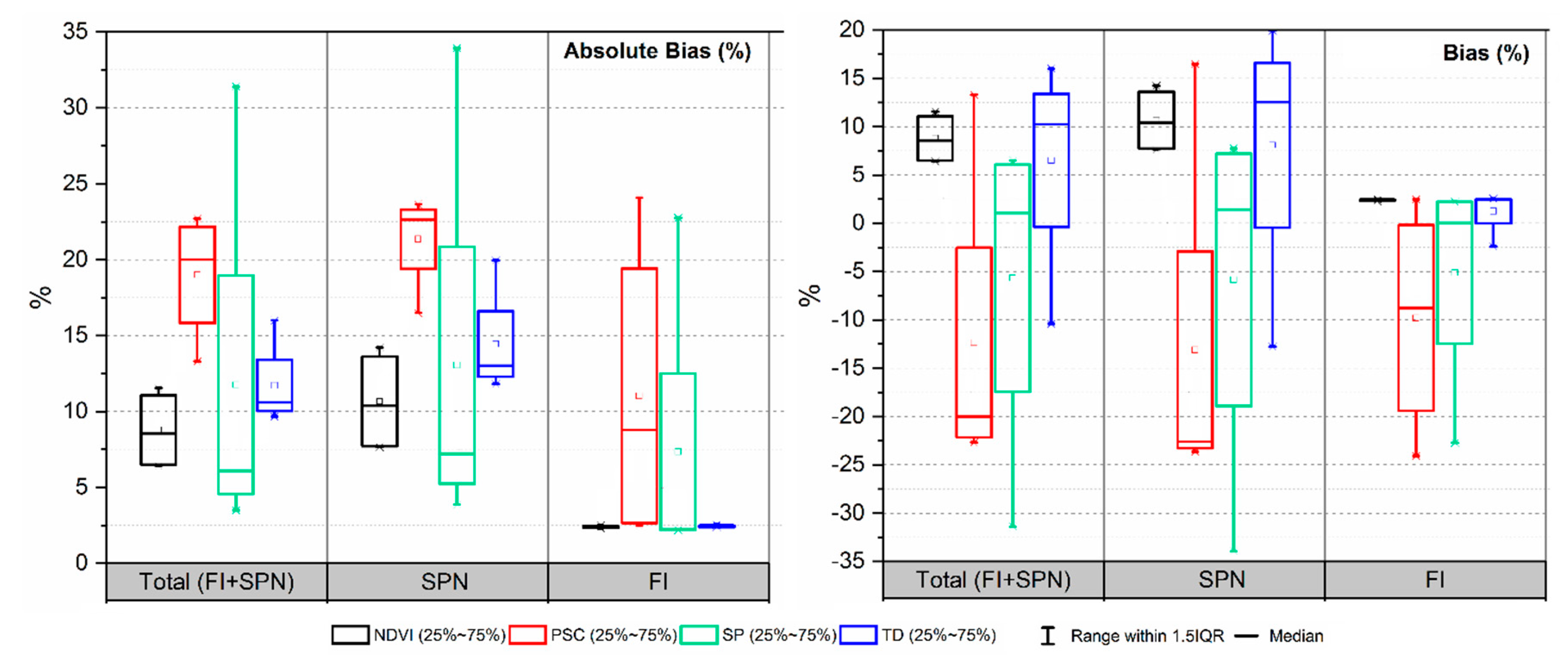
4.6. Cross-Validation of Results

In order to test the robustness of the analysis and check the stability of the performance of all 16 methods for mapping of vegetation in other parts of Antarctica, we cross-validated our results against data from the Schirmacher Oasis. This analysis was necessary to test the applicability of the present analysis in other parts of Antarctica for mapping vegetation. The cross-validation site was selected on the basis of availability of WV-2 data (05 February 2012) and supporting ground truth data collected during Indian Scientific Expeditions to Antarctica (2011–12). The Schirmacher Oasis is a ∼35 km long and up to 3 km wide ice-free plateau located on the Princess Astrid Coast of Queen Maud Land, East Antarctica, with a low-lying hilly topography. The presence of more than 100 freshwater lakes and numerous meltwater streams in the Schirmacher Oasis provide suitable habitat for the growth of bryophytes. The flora of the Schirmacher Oasis is entirely cryptogamic, including algae, fungi, lichens, and mosses. Our cross-validation procedure confirmed the major results of our rigorous experiment, including the superior performance of five methods (MTMF, MF/SAM, MF, NDVI-2, NDVI-4) among the 16 candidate methods. RedEdge-based NDVIs again proved their robustness as compared to red band-based NDVIs. The NDVI approach again proved to be the most stable, providing consistent results in mapping vegetation. The final vegetation map of the Schirmacher Oasis derived by using these top five methods is depicted in Figure 11. These cross-validation results confirm the validity of extending the approach of this study to other parts of Antarctica.

5. Discussion

5.1. Performance of Semi-Automatic Mapping Methods

Spectral processing and target detection mixed tuned methods (MTMF and MT-TCIMF) consistently achieved the lowest number of false assessments for all sizes of vegetation patches. This is consistent with the findings of [75], which suggested that, if the spectral angle between the target (here vegetation) and the non-target (background confounding features) is significant, TCIMF/MT-TCIMF can considerably reduce the number of false positives when compared with the CEM detector. Amongst the 16 methods examined here, apart from MTMF methods and NDVI-2/NDVI-4, the MF/SAM (misclassified pixels = 5.64%) and MF (misclassified pixels = 6.50%) methods showed great vegetation visibility by suppressing false signals, resulting in low bias values in extracted vegetation areas when compared with other methods. Based on the misclassified vegetation pixels computed from the number of false positives, MT-TCIMF and ACE performed better than the customized NDVI methods (NDVI-1 and NDVI-3) and all four methods in the pixel-wise supervised classification approach. We also found that the MF/SAM ratio significantly suppressed the false positives when using either MF or SAM, while improving the detection of the true positives. For instance, if a pixel with vegetation had a high MF and low SAM value (low SAM value represents high probability of being a target pixel), the ratio (MF/SAM) would generate a high true positive. In contrast, if the MF had a high value for a false positive, but the SAM classified it as a non-vegetated pixel (high SAM value), the ratio would be lower, reducing the chance of a false positive.

Overall, the visual images of extracted vegetation regions using four feature extraction approaches indicated that most of the misclassification occurred at shadow-prone and topographically varying areas (Figure 5 and Supplementary Figures S3–S6). We also noted outliers (highlighted in Table 4, Table 5 and Supplementary Table S4) relating to overestimating methods, including two pixel-wise supervised classification methods (MXL and NNC), spectral processing (PCA) and target detection (ACE), which produced erratically higher false positives and higher overestimation of vegetation. Global outliers (with respect to the 16 methods) and local outliers (with respect to the four general methods in the approach) are highlighted in Table 4, Table 5, and Supplementary Table S4. Outliers were calculated based on interquartile range (IQR) (i.e., Tukey’s fences) in which Q₁ and Q₃ are the lower and upper quartiles respectively, and outlier was defined as any value outside the range: [Q₁-k(Q₃-Q₁), Q₃+k(Q₃-Q₁)], where k = 1.5. The occurrence of outliers was related to excessive overestimation of vegetation by these methods, while methods leading to underestimation were free from outliers in misclassification. The overestimations in these methods appear to be caused by confounding signatures of background features, leading to failure to model the background appropriately. Our results are also consistent with previous studies confirming the poor performance of PCA and MXL [72,76,87,88], and confirm that non-parametric methods such as SVM are well suited to VHR compared to parametric methods such as MXL [89]. The NDVI approach in the present study did not suffer from outliers and hence performed consistently throughout the experiment.

5.2. Effect of Spectral-Spatial Resolution nn Sparse Vegetation Mapping

The usefulness of RedEdge bands and spectral indices based on RedEdge bands for vegetation health monitoring has been previously reported [90,91,92,93]. However, the availability of RedEdge band and related improvement in vegetation mapping is still a topic of active debate. This is mainly because few studies have demonstrated improved accuracy of vegetation mapping by using RedEdge bands (e.g., [94]), and others have found only limited improvement in vegetation mapping (e.g., [95,96]), while some did not report any significant improvements (e.g., [97]). In the cryospheric environment, Zagajewski et.al. [98] demonstrated the effectiveness of RapidEye RedEdge band-based NDVI to study High Arctic vegetation. In the present study, we have implemented four NDVIs (two with red bands and two with RedEdge bands). Similar to previous studies [92,93,99] conducted in various geographical regions, our results confirm that RedEdge NDVIs provide slightly improved results in comparison to the traditional red band VIs in mapping cryospheric vegetation.

Currently, there are a very few satellite sensors with RedEdge band availability, including RapidEye (launched in 2008, GSD = 6.5 m, RedEdge spectral range = 690–730 nm), Sentinel-2 (launched in 2015, GSD = 20 m, with three RedEdge bands, band 5 spectral range 694–714 nm, band 6 spectral range 731–749 nm, and band 7 spectral range 768–796 nm), and Worldview-2 (launched in 2009, GSD = 1.80 m, RedEdge spectral range 705–745 nm). Based on the proven effectiveness of the RedEdge band in vegetation mapping, its possible inclusion in the Landsat-10 mission is under active consideration [100]. The RapidEye and WV-2/3 provide a VHR RedEdge band, but these datasets are expensive for long-term regional vegetation mapping in Antarctica, often lack consistent global coverage, while these satellites also acquire data on specific missions making historical data for many areas unattainable. Sentinel-2 provides medium resolution RedEdge band, but it does not have a long-term historical archive and consequently cannot be used for a long-term time series analysis. All these satellites with RedEdge bands can be used for mapping vegetation in various types of environments, for instance in urban, forest, and agricultural areas. However, it has been shown that spatial resolution can paradoxically be both beneficial or adverse to classification, depending on the land type being classified, and that accuracy is dependent on class spectral variance, at different spatial scales [101,102]. In the present study, because of small, patchy, and sparse vegetation sizes, use of Sentinel-1 RedEdge to map vegetation from Antarctica might not be effective and precise. However, Sentinel-1 (with RedEdge and five days revisit time) and Landsat images (lacks RedEdge with 16 days revisit time) can be used to map vegetation in some parts of Antarctica (e.g., Antarctic Peninsula) where vegetation patches are comparable to the spatial resolution of satellite images [19]. Both Sentinel and Landsat data are freely available. Using RedEdge-based spectral indices derived from medium resolution satellite imageries would lead to considerable underestimation of vegetation as the spatial resolution will be insufficient to map smaller vegetation patches. In order to map continent-wide vegetation extent using spectral indices derived in the present study, high-resolution RedEdge band satellites with consistent coverage will be effective. Continuous availability of these satellite images will also be useful for mapping spatio-temporal changes in vegetation in Antarctica, which can then be linked to the response of vegetation to the warming and other environmental changes in the continent.

5.3. Comparison of Results with Previous Case Studies Dealing with Vegetation Mapping in Cryospheric Environments

MTMF-based classification of tundra–taiga vegetation in the Tuliok River, Khibiny Mountains, Russia, using QuickBird and Terra ASTER image yielded an accurate vegetation map [103]. Similar robust results in vegetation mapping were derived in the present study demonstrating the effectiveness of MTMF in cryospheric vegetation mapping. Mikola et al. [104] demonstrated the effectiveness of using NDVI to study the spatial variation of vegetation characteristics in Siberian Arctic tundra using multitemporal WV-2 and QuickBird data. On a similar note, our research confirms customized NDVI as a robust tool for mapping cryospheric vegetation. Suchá et al. [105] compared the suitability of multispectral data with different spatial and spectral resolutions for classifications of tundra vegetation in the Krkonoše Mts. National Park using WV-2 and Landsat 8 data using object-based classification and traditional pixel-based classifiers (MXL, SVM, and NN). Mapping of tundra vegetation using WV-2 data yielded best results using the object-based approach (68.4%), while pixel-based SVM classification yielded 60.82% accuracy. On the other hand, Landsat-based classification of tundra vegetation using MXL yielded the best accuracy of 78.31%. Similarly, in the present study, SVM was the superior of the four pixel-based classifiers, which shows that our results are consistent with previous studies conducted in similar cryospheric environments [105,106]. Consistent with the attempt by Suchá et al. [105], our study also concludes that high spatial resolution of WV-2 is the significant feature essential to reach high overall classification accuracy in vegetation mapping.

In most previous studies, medium or coarse resolution data were used to map vegetation—a resolution too coarse to analyze Larsemann Hills vegetation. Because of its patchy and sparse nature with fuzzy boundaries, almost all of the areas on the Larsemann Hills would show as non-vegetated using medium or coarse resolution satellite datasets. On the other hand, the very high spatial resolution of WV-2 (0.5 m) used in this study evidently identified the presence of even isolated vegetated patches of size 0.25 m². Using the high-resolution imagery, the present study was successful in precisely mapping fuzzy boundaries of vegetation patches from the study area. Given that our Antarctic vegetation mapping method is based on physical principles of spectral remote sensing, it could be modified to other low density/fragmented/patchy short-stature plant communities (e.g., tundra grasslands), including mountainous/alpine and desert regions (arid and semi-arid landscapes). Therefore, this analysis shows potential to develop into an operational component of vegetation mapping from remote areas.

5.4. Challenges in Vegetation Mapping in Cryospheric Environments

The present study provides a broad overview of the challenges and practical issues in mapping sparse vegetation and way forward to deal with these challenges. Several factors contribute to effective mapping of sparse vegetation: (1) Robust operational mapping of sparse vegetation needs multitemporal, multi-seasonal, high spatial resolution, and reliable spectral resolution VHR data coupled with real time ground truth data collection; however, this is practically very difficult or impossible in remote areas such as Svalbard, Greenland, or Antarctica. (2) Spectral responses of sparse vegetation patches are mixed with the background soil/snow cover/rocks (mixed pixels or mixels) as they sometimes do not cover the entire pixel [107]. In a few cases, the entire vegetated patch may not visible because of melting ice or snow cover. Snow- or ice-covered vegetation patches can be identified using VHR polarimetric synthetic aperture radar (SAR) data because of their capabilities to penetrate the snow cover. Mapping of snow-covered vegetated patches is beyond the scope of the present study. (3) Cloud cover, varying weather conditions, and shadows in multispectral data are also limiting factors in vegetation mapping [105]. Availability of multispectral data of polar regions is limited by the frequent cloud cover in summer, low sun angle, and topographical constraints resulting in extended shadow cover. (4) Vegetation mapping results can also be influenced by varying seasons. For instance, tundra vegetation structures tend to be compact during spring and autumn, while in summer various vegetation structures (e.g., grassland) tend to grow and form a mixture [105]. Unfortunately, it is almost impossible to obtain VHR data of suitable spectral-spatial resolution within one season to track these changes. (6) Add-on spectral bands of WV-2 provide significant differences in spectral response for the different colors of vegetation forms which are useful for mapping vegetation patches. However, similar studies should be conducted using a limited number of spectral bands to confirm the effect of spectral range on vegetation mapping. (7) Training data for executing classification methods is the most crucial input for any supervised method. Defining ROIs is crucial considering smaller patches of vegetation, as improper selection of ROIs will lead to overall errors in classification. To avoid such errors, we have used ground truth data as well as manual interpretation of VHR imagery. (8) VI values can be erroneous because of soil type [19], which is especially challenging in soils with high organic content where, for instance, NDVI values can increase in areas of peaty soils [19]. In Antarctica, a large majority of soils are minerogenic, with very little organic matter, and therefore, we found no evidence of this effect here.

5.5. Experimental Limitations of the Present Study and a Way Forward

In this study, we used four feature extraction approaches simply to detect the presence of vegetation and assess its spatial extent at refined scale. The use of such approaches in quantitative ecology to estimate verdancy, species richness, and biomass is beyond the scope of this study and would require consideration of many other factors. The polygons extracted as vegetated in this study contained uneven amounts of various vegetation forms (various species of moss, lichens, and algae). However, in this study, no measurement was made of percentage contribution of each vegetation component, and therefore we cannot quantify the density of each form/species within each polygon. Future experiments will be conducted to examine whether these feature extraction methods can differentiate and map different species of vegetation. In addition, conducting a temporal analysis of vegetation based on compiling time series of vegetation maps from the literature is beyond the scope of this study; however, simple comparison of our estimate of vegetated areas with ground surveyed results may highlight the effects of spatial resolution on the extraction of vegetation. For a reliable analysis of long-term temporal vegetation changes and for mapping species configuration (and even quantifying surface stress factors), satellite data should be acquired for the study area by using RapidEye and WV-3 sensors with similar band configuration. Moreover, quantifying factors responsible for the winter-time stress of vegetation and its vitality in summer should also be documented in future studies, as done elsewhere [98].

In this study, the ground-truthing was conducted during the austral summer periods (December to March) of 2011–2015, and the WV-2 image acquisition was carried out on February 9, 2011. Therefore, there is a varying (a few days to few weeks) temporal difference between the vegetation mapped using WV-2 (2011) and the actual ground survey. This short temporal difference can introduce some error into our analyses as vegetation cover can change in physical (compactness) and biological (pigmentation) appearance within short periods. Within a few days to few weeks, moss cover can change from a healthy (appearance: green open-leaved form) to a stress-resisting denser (appearance: yellow-brown or red) form. However, we assume the vegetation growth over the present study area during the austral summer of 2011–12 to be very slow; therefore, it would cause a minor influence on the present analysis and can be considered as a minor unquantifiable possible source of error in the present study. To account for temporal changes in vegetation in the short period of the summer season, it is recommended that the multiple WV-2 image acquisitions should be completed during December–March to compensate for any temporal changes in vegetation cover. Synergism of more detailed ground truth survey, real-time VHR data acquisition, and use of high-performing feature extraction methods give the prospect of providing better information on vegetation cover with the contribution of different terrestrial vegetation. If this prospect can be achieved, it would essentially provide new ways of monitoring not only vegetation extent but also compositional (vegetation types and species) change in this region.

6. Conclusions

In this study, we focused on generating a vegetation mapping dataset of the Larsemann Hills region using high spatial resolution PAN-sharpened WV-2 images and 16 pixel-based image classification methods including thresholds based on band ratios. This research has confirmed and demonstrated that WV-2 imagery contains sufficient spectral information to allow differentiation and mapping of vegetation from the surrounding landmass. Benefits of using WV-2 images for fine-scale vegetation mapping have previously been reported in various environments by other studies. However, this is the first time that WV-2 has been exclusively used for fine-scale mapping of vegetation in Antarctica, confirming the effectiveness of this imagery in cryospheric landscapes. With the 0.5 m resolution WV-2 images, we have numerically delineated vegetation patches in the Larsemann hills and environs in unprecedented detail. The overall ranking of accuracy for the 16 vegetation extraction methods was: MTMF > MF/SAM > NDVI-2 > MF > NDVI-4 > MT-TCIMF > ACE > NDVI-3 > OSP > NDVI-1 > SAM > CEM > SVM > NNC > MXL > PCA. Based on overall comparison of the individual methods, we recommend the five top-performing methods MTMF, MF/SAM, MF, NDVI-2, and NDVI-4 for future vegetation mapping studies. The total area (average) of vegetation mapped in the study area using an ensemble of the five top-performing methods is estimated to be 662,892.19 ± 12,143.33 m² for Fisher Island, 2,194,161.28 ± 43,658.09 m² for Stornes Peninsula and 1,623,055.22 ± 27,792.91 m² for Schirmacher Oasis. The vegetation dataset presented in this study is the first precise and refined map covering the Larsemann Hills region derived from WV-2 data and provides the baseline information required for future temporal change analysis of the vegetation in this region.

References

1. Turner, J.; Bindschadler, R.A.; Convey, P.; di Prisco, G.; Fahrbach, E.; Gutt, J.; Hodgson, D.A.; Mayewski, P.A.; Summerhayes, C.P. Antarctic Climate Change and the Environment (ACCE); Scientific Committee on Antarctic Research: Cambridge, UK, 2009; p. 526. [Google Scholar]
2. Turner, J.; Barrand, N.; Bracegirdle, T.; Convey, P.; Hodgson, D.; Jarvis, M.; Jenkins, A.; Marshall, G.; Meredith, M.; Roscoe, H.; et al. Antarctic climate change and the environment: An update. Polar Record 2013, 50, 237–259. [Google Scholar] [CrossRef]
3. Convey, P. Antarctic terrestrial biodiversity in a changing world. Polar Biol. 2011, 34, 1629–1641. [Google Scholar] [CrossRef]
4. Smith, R.I.L. Terrestrial biology of the Antarctic and subAntarctic. In Antarctic Ecology, 2nd ed.; Laws, R.M., Ed.; Academic Press: London, UK, 1984; p. 61e162. [Google Scholar]
5. Longton, R. The Biology of Polar Bryophytes and Lichens; CUP Archive: Cambridge, UK, 1988. [Google Scholar]
6. Convey, P.; Chown, S.; Clarke, A.; Barnes, D.; Bokhorst, S.; Cummings, V.; Ducklow, H.; Frati, F.; Green, T.; Gordon, S.; et al. The spatial structure of Antarctic biodiversity. Ecol. Monogr. 2014, 84, 203–244. [Google Scholar] [CrossRef] [Green Version]
7. Simms, É.; Ward, H. Multisensor NDVI-based monitoring of the tundra-taiga interface (Mealy Mountains, Labrador, Canada). Remote Sens. 2013, 5, 1066–1090. [Google Scholar] [CrossRef]
8. Cannone, N.; Dalle Fratte, M.; Convey, P.; Worland, M.R.; Guglielmin, M. Ecology of moss banks at Signy Island (maritime Antarctica). Bot. J. Linnean Soc. 2017, 184, 518–533. [Google Scholar] [CrossRef]
9. Cannone, N.; Guglielmin, M.; Convey, P.; Worland, M.R.; Favero Longo, S.E. Vascular plant changes in extreme environments: Effects of multiple drivers. Clim. Chang. 2016, 134, 651–665. [Google Scholar] [CrossRef]
10. Convey, P.; Bindschadler, R.; di Prisco, G.; Fahrbach, E.; Gutt, J.; Hodgson, D.; Mayewski, P.; Summerhayes, C.; Turner, J. Antarctic climate change and the environment. Antarctic Sci. 2009, 21, 541. [Google Scholar] [CrossRef]
11. Fowbert, J.A.; Smith, R.I.L. Rapid population increase in native vascular plants in the Argentine Islands, Antarctic Peninsula. Arctic Alpine Res. 1994, 26, 290–296. [Google Scholar] [CrossRef]
12. Parnikoza, I.; Convey, P.; Dykyy, I.; Trakhimets, V.; Milinevsky, G.; Tyschenko, O.; Inozemtseva, D.; Kozeretska, I. Current status of the Antarctic herb tundra formation in the central Argentine Islands. Glob. Chang. Biol. 2009, 15, 1685–1693. [Google Scholar] [CrossRef]
13. Robinson, S.; Wasley, J.; Tobin, A. Living on the edge - plants and global change in continental and maritime Antarctica. Global Chang. Biol. 2003, 9, 1681–1717. [Google Scholar] [CrossRef] [Green Version]
14. Turner, D.; Lucieer, A.; Malenovský, Z.; King, D.; Robinson, S. Spatial co-registration of ultra-high resolution visible, multispectral and thermal images acquired with a micro-UAV over Antarctic Moss Beds. Remote Sens. 2014, 6, 4003–4024. [Google Scholar] [CrossRef]
15. Lucieer, A.; Turner, D.; King, D.; Robinson, S. Using an Unmanned Aerial Vehicle (UAV) to capture micro-topography of Antarctic moss beds. Int. J. Appl. Earth Obs. Geoinformat. 2014, 27, 53–62. [Google Scholar] [CrossRef] [Green Version]
16. Bricher, P.; Lucieer, A.; Shaw, J.; Terauds, A.; Bergstrom, D. Mapping sub-antarctic cushion plants using random forests to combine very high resolution satellite imagery and terrain modelling. PLoS ONE 2013, 8, e72093. [Google Scholar] [CrossRef] [PubMed]
17. Laidler, G.; Treitz, P.; Atkinson, D. Remote sensing of arctic vegetation: Relations between the NDVI, spatial resolution and vegetation cover on Boothia Peninsula, Nunavut. ARCTIC 2008, 61, 1. [Google Scholar] [CrossRef]
18. Bhatt, U.; Walker, D.; Raynolds, M.; Comiso, J.; Epstein, H.; Jia, G.; Gens, R.; Pinzon, J.; Tucker, C.; Tweedie, C.; et al. Circumpolar arctic tundra vegetation change is linked to sea ice decline. Earth Interact. 2010, 14, 1–20. [Google Scholar] [CrossRef]
19. Fretwell, P.; Convey, P.; Fleming, A.; Peat, H.; Hughes, K. Detecting and mapping vegetation distribution on the Antarctic Peninsula from remote sensing data. Polar Biol. 2011, 34, 273–281. [Google Scholar] [CrossRef]
20. Malenovský, Z.; Lucieer, A.; King, D.; Turnbull, J.; Robinson, S. Unmanned aircraft system advances health mapping of fragile polar vegetation. Methods Ecol. Evolut. 2017, 8, 1842–1857. [Google Scholar] [CrossRef] [Green Version]
21. Murray, H.; Lucieer, A.; Williams, R. Texture-based classification of sub-Antarctic vegetation communities on Heard Island. Int. J. Appl. Earth Obs. Geoinformat. 2010, 12, 138–149. [Google Scholar] [CrossRef]
22. Casanovas, P.; Black, M.; Fretwell, P.; Convey, P. Mapping lichen distribution on the Antarctic Peninsula using remote sensing, lichen spectra and photographic documentation by citizen scientists. Polar Res. 2015, 34, 25633. [Google Scholar] [CrossRef]
23. Shin, J.; Kim, H.; Kim, S.; Hong, S. Vegetation abundance on the Barton Peninsula, Antarctica: Estimation from high-resolution satellite images. Polar Biol. 2014, 37, 1579–1588. [Google Scholar] [CrossRef]
24. Markon, C.; Derksen, D. Identification of tundra land cover near Teshekpuk Lake, Alaska Using SPOT Satellite Data. ARCTIC 1994, 47, 222–231. [Google Scholar] [CrossRef]
25. Griffith, B.; Douglas, C.D.; Noreen, E.; Donald, W.; Young, D.; Mccabe, T.R.; Russell, D.E.; White, R.G.; Cameron, R.D.; Whitten, R.K. The Porcupine Caribou Herd. In Biological Science Report; USGS/BRD: Reston, VA, USA, 2002. [Google Scholar]
26. Walker, D.; Raynolds, M.; Daniëls, F.; Einarsson, E.; Elvebakk, A.; Gould, W.; Katenin, A.; Kholod, S.; Markon, C.; Melnikov, E.; et al. The other members of the CAVM Team. The Circumpolar Arctic vegetation map. J. Vegetat. Sci. 2005, 16, 267–282. [Google Scholar] [CrossRef]
27. Lindblad, K.; Nyberg, R.; Molau, U. Generalization of heterogeneous alpine vegetation in air photo-based image classification, Latnjajaure catchment, northern Sweden. Pirineos 2006, 161, 3–32. [Google Scholar] [CrossRef]
28. Karlsen, R.; Malnes, E.; Haarpaintner, J.; Solberg, R. Mapping and modelling the snowmelt and greening pattern in southern Norway by combining microwave and optical remote sensing sensors. In Proceedings of the IEEE International Geoscience and Remote Sensing Symposium IGARSS, Barcelona, Spain, 23–28 July 2007. [Google Scholar]
29. Schneider, J.; Grosse, G.; Wagner, D. Land cover classification of tundra environments in the Arctic Lena Delta based on Landsat 7 ETM+ data and its application for upscaling of methane emissions. Remote Sens. Environ. 2009, 113, 380–391. [Google Scholar] [CrossRef] [Green Version]
30. Raynolds, M.; Walker, D.; Epstein, H.; Pinzon, J.; Tucker, C. A new estimate of tundra-biome phytomass from trans-Arctic field data and AVHRR NDVI. Remote Sens. Lett. 2011, 3, 403–411. [Google Scholar] [CrossRef]
31. Atkinson, D.; Treitz, P. Arctic Ecological Classifications Derived from Vegetation Community and Satellite Spectral Data. Remote Sens. 2012, 4, 3948–3971. [Google Scholar] [CrossRef] [Green Version]
32. Ullmann, T.; Schmitt, A.; Roth, A.; Duffe, J.; Dech, S.; Hubberten, H.; Baumhauer, R. Land Cover Characterization and Classification of Arctic Tundra Environments by Means of Polarized Synthetic Aperture X- and C-Band Radar (PolSAR) and Landsat 8 Multispectral Imagery—Richards Island, Canada. Remote Sens. 2014, 6, 8565–8593. [Google Scholar] [CrossRef]
33. Bratsch, S.; Epstein, H.; Buchhorn, M.; Walker, D. Differentiating among Four Arctic Tundra Plant Communities at Ivotuk, Alaska Using Field Spectroscopy. Remote Sens. 2016, 8, 51. [Google Scholar] [CrossRef]
34. Black, M.; Casanovas, P.; Convey, P.; Fretwell, P. High Resolution mapping of Antarctic vegetation communities using airborne Hyperspectral data. In Proceedings of the RSPSOC, Aberystwyth, UK, 2–15 September 2014. [Google Scholar] [CrossRef]
35. Buchhorn, M.; Walker, D.; Heim, B.; Raynolds, M.; Epstein, H.; Schwieder, M. Ground-based hyperspectral characterization of Alaska tundra vegetation along environmental gradients. Remote Sens. 2013, 5, 3971–4005. [Google Scholar] [CrossRef]
36. Dalmayne, J.; Möckel, T.; Prentice, H.; Schmid, B.; Hall, K. Assessment of fine-scale plant species beta diversity using WorldView-2 satellite spectral dissimilarity. Ecol. Informat. 2013, 18, 1–9. [Google Scholar] [CrossRef]
37. Liu, N.; Treitz, P. Modelling high arctic percent vegetation cover using field digital images and high resolution satellite data. Int. J. Appl. Earth Obs. Geoinformat. 2016, 52, 445–456. [Google Scholar] [CrossRef]
38. Davidson, S.; Santos, M.; Sloan, V.; Watts, J.; Phoenix, G.; Oechel, W.; Zona, D. Mapping Arctic Tundra Vegetation Communities Using Field Spectroscopy and Multispectral Satellite Data in North Alaska, USA. Remote Sens. 2016, 8, 978. [Google Scholar] [CrossRef]
39. Liu, N.; Budkewitsch, P.; Treitz, P. Examining spectral reflectance features related to Arctic percent vegetation cover: Implications for hyperspectral remote sensing of Arctic tundra. Remote Sens. Environ. 2017, 192, 58–72. [Google Scholar] [CrossRef]
40. Juutinen, S.; Virtanen, T.; Kondratyev, V.; Laurila, T.; Linkosalmi, M.; Mikola, J.; Nyman, J.; Räsänen, A.; Tuovinen, J.; Aurela, M. Spatial variation and seasonal dynamics of leaf-area index in the arctic tundra-implications for linking ground observations and satellite images. Environ. Res. Lett. 2017, 12, 095002. [Google Scholar] [CrossRef]
41. Gould, W.; Edlund, S.; Zoltai, S.; Raynolds, M.; Walker, D.; Maier, H. Canadian Arctic vegetation mapping. Int. J. Remote Sens. 2002, 23, 4597–4609. [Google Scholar] [CrossRef]
42. Guay, K.; Beck, P.; Berner, L.; Goetz, S.; Baccini, A.; Buermann, W. Vegetation productivity patterns at high northern latitudes: A multi-sensor satellite data assessment. Global Chang. Biol. 2014, 20, 3147–3158. [Google Scholar] [CrossRef]
43. Stow, D.; Hope, A.; McGuire, D.; Verbyla, D.; Gamon, J.; Huemmrich, F.; Houston, S.; Racine, C.; Sturm, M.; Tape, K.; et al. Remote sensing of vegetation and land-cover change in Arctic Tundra Ecosystems. Remote Sens. Environ. 2004, 89, 281–308. [Google Scholar] [CrossRef] [Green Version]
44. McFadden, J.; Chapin, F.; Hollinger, D. Subgrid-scale variability in the surface energy balance of arctic tundra. J. Geophys. Res. Atmos. 1998, 103, 28947–28961. [Google Scholar] [CrossRef]
45. Raynolds, M.; Walker, D.; Maier, H. NDVI patterns and phytomass distribution in the circumpolar Arctic. Remote Sens. Environ. 2006, 102, 271–281. [Google Scholar] [CrossRef]
46. Hodgson, D.; Noon, P.; Vyverman, W.; Bryant, C.; Gore, D.; Appleby, P.; Gilmour, M.; Verleyen, E.; Sabbe, K.; Jones, V.; et al. Were the Larsemann Hills ice-free through the Last Glacial Maximum? Antarctic Sci. 2001, 13, 440–454. [Google Scholar] [CrossRef] [Green Version]
47. Hodgson, D.; Verleyen, E.; Sabbe, K.; Squier, A.; Keely, B.; Leng, M.; Saunders, K.; Vyverman, W. Late Quaternary climate-driven environmental change in the Larsemann Hills, East Antarctica, multi-proxy evidence from a lake sediment core. Quat. Res. 2005, 64, 83–99. [Google Scholar] [CrossRef]
48. Antarctic Treaty Consultative Meeting (ATCM). XXXVII—CEP XVII Final Report, Management Plan for Antarctic Specially Protected Area No. 174: Stornes, Larsemann Hills, Princess Elizabeth Land (Measure 12) and Larsemann Hills, East Antarctica Antarctic Specially Managed Area Management Plan (Measure 15), 28 April–7 May 2014, Brasilia, Brazil. Available online: https://www.ats.aq/documents/recatt/att555_e.pdf (accessed on 6 July 2017).
49. Jawak, S.; Luis, A. Synergistic use of multitemporal RAMP, ICESat and GPS to construct an accurate DEM of the Larsemann Hills region, Antarctica. Adv. Space Res. 2012, 50, 457–470. [Google Scholar] [CrossRef]
50. Harris, U. Larsemann Hills—Mapping from Aerial Photography Captured February 1998, Australian Antarctic Data Centre—CAASM Metadata, 2002, (Updated 2014). Available online: http://data.aad.gov.au/aadc/metadata/ (accessed on 6 July 2015).
51. Paul, F.; Kääb, A. Perspectives on the production of a glacier inventory from multispectral satellite data in Arctic Canada: Cumberland Peninsula, Baffin Island. Ann. Glacio. 2005, 42, 59–66. [Google Scholar] [CrossRef] [Green Version]
52. Congalton, R. A review of assessing the accuracy of classifications of remotely sensed data. Remote Sens. Environ. 1991, 37, 35–46. [Google Scholar] [CrossRef]
53. Congalton, R.; Green, K. Assessing the accuracy of remotely sensed data. In Mapping Science; CRC Press: Boca Raton, FL, USA, 2008. [Google Scholar]
54. Santos, T.; Freire, S. Testing the Contribution of WorldView-2 Improved Spectral Resolution for Extracting Vegetation Cover in Urban Environments. Can. J. Remote Sens. 2015, 41, 505–514. [Google Scholar] [CrossRef]
55. Jawak, S.; Luis, A. A spectral index ratio-based Antarctic land-cover mapping using hyperspatial 8-band WorldView-2 imagery. Polar Sci. 2013, 7, 18–38. [Google Scholar] [CrossRef] [Green Version]
56. DigitalGlobe. The Benefits of the Eight Spectral Bands of WorldView-2, White Paper (WP-8SPEC) 2010, Rev 01/13. Available online: http://www.geoimage.com.au/CaseStudies/TheBenefits_8BandData.pdf (accessed on 6 July 2014).
57. Digital Globe. Radiometric Use of WorldView-2 Imagery. 2012. Available online: www.digitalglobe.com/downloads/Radiometric_Use_of_WorldView-2_Imagery.pdf (accessed on 6 July 2014).
58. Richter, R.; Schläpfer, D. Atmospheric/Topographic Correction for Satellite Imagery; DLR Report DLR-IB 565-01/05; DLR: Wessling, Germany, 2011. [Google Scholar]
59. Johnson, B. Effects of Pansharpening on Vegetation Indices. ISPRS Int. J. Geo-Inf. 2014, 3, 507–522. [Google Scholar] [CrossRef]
60. Jawak, S.; Luis, A. A Comprehensive Evaluation of PAN-Sharpening Algorithms Coupled with Resampling Methods for Image Synthesis of Very High Resolution Remotely Sensed Satellite Data. Adv. Remote Sens. 2013, 2, 332–344. [Google Scholar] [CrossRef] [Green Version]
61. Tucker, C. Red and photographic infrared linear combinations for monitoring vegetation. Remote Sens. Environ. 1979, 8, 127–150. [Google Scholar] [CrossRef] [Green Version]
62. Jackson, R.; Huete, A. Interpreting vegetation indices. Prevent. Vet. Med. 1991, 11, 185–200. [Google Scholar] [CrossRef]
63. Myneni, R.; Hall, F.; Sellers, P.; Marshak, A. The interpretation of spectral vegetation indexes. IEEE Trans. Geosci. Remote Sens. 1995, 33, 481–486. [Google Scholar] [CrossRef]
64. Rouse, J.W.; Haas, R.H.; Schell, J.A.; Deering, D.W. Monitoring vegetation systems in the Great Plains with ERTS. In Proceedings of the 3rd Earth Resource Technology Satellite (ERTS) Symposium, NASA, Washington, DC, USA, 1 January 1974; pp. 309–317. [Google Scholar]
65. Huete, A. A soil-adjusted vegetation index (SAVI). Remote Sens. Environ. 1988, 25, 295–309. [Google Scholar] [CrossRef]
66. Kim, M.S.; Daughtry, C.S.T.; Chappelle, E.W.; McMurtrey, J.E.; Walthall, C.L. The use of high spectral resolution bands for estimating absorbed photosynthetically active radiation. In Proceedings of the 6th Symposium on Physical Measurements and Signatures in Remote Sensing, Val d’Isere, France, 1 January 1994; pp. 299–306. [Google Scholar]
67. Daughtry, C. Estimating Corn Leaf Chlorophyll Concentration from Leaf and Canopy Reflectance. Remote Sens. Environ. 2000, 74, 229–239. [Google Scholar] [CrossRef]
68. Roujean, J.; Breon, F. Estimating PAR absorbed by vegetation from bidirectional reflectance measurements. Remote Sens. Environ. 1995, 51, 375–384. [Google Scholar] [CrossRef]
69. Broge, N.; Leblanc, E. Comparing prediction power and stability of broadband and hyperspectral vegetation indices for estimation of green leaf area index and canopy chlorophyll density. Remote Sens. Environ. 2001, 76, 156–172. [Google Scholar] [CrossRef]
70. Gitelson, A.; Merzlyak, M.N. Signature Analysis of Leaf Reflectance Spectra: Algorithm Development for Remote Sensing of Chlorophyll. J. Plant Physiol. 1996, 148, 494–500. [Google Scholar] [CrossRef]
71. Xiaocheng, Z.; Tamas, J.; Chongcheng, C.; Malgorzata, W.V. Urban land cover mapping based on object oriented classification using worldview 2 satellite remote sensing images. In Proceedings of the International Scientific Conference on Sustainable Development & Ecological Footprint, Sopron, Hungary, 25–26 March 2012. [Google Scholar]
72. Jawak, S.; Luis, A. A semiautomatic extraction of antarctic lake features using worldview-2 imagery. Photogramm. Eng. Remote Sens. 2014, 80, 939–952. [Google Scholar] [CrossRef]
73. Wolf, A. Using WorldView-2 Vis-NIR multispectral imagery to support land mapping and feature extraction using normalized difference index ratios. In Proceedings of the SPIE 8390, Algorithms and Technologies for Multispectral, Hyperspectral, and Ultraspectral Imagery XVIII, Baltimore, MD, USA, 23–27 April 2012. [Google Scholar]
74. Peng, H.; Fuhui Long, F.; Ding, C. Feature selection based on mutual information criteria of max-dependency, max-relevance, and min-redundancy. IEEE Trans. Pattern Anal. Mach. Intell. 2005, 27, 1226–1238. [Google Scholar] [CrossRef]
75. Jin, X.; Paswaters, S.; Cline, H. A comparative study of target detection algorithms for hyperspectral imagery. In Proceedings of the SPIE 7334, Algorithms and Technologies for Multispectral, Hyperspectral, and Ultraspectral Imagery XV, Orlando, FL, USA, 27 April 2009. [Google Scholar]
76. Jawak, S.; Luis, A. Very high-resolution satellite data for improved land cover extraction of Larsemann Hills, Eastern Antarctica. J. Appl. Remote Sens. 2013, 7, 073460. [Google Scholar] [CrossRef]
77. Harsanyi, J.; Chang, C. Hyperspectral image classification and dimensionality reduction: An orthogonal subspace projection approach. IEEE Trans. Geosci. Remote Sens. 1994, 32, 779–785. [Google Scholar] [CrossRef]
78. Bourennane, S.; Fossati, C.; Cailly, A. Improvement of Target-Detection Algorithms Based on Adaptive Three-Dimensional Filtering. IEEE Trans. Geosci. Remote Sens. 2011, 49, 1383–1395. [Google Scholar] [CrossRef]
79. Chang, C.; Liu, J.; Chieu, B.; Ren, H.; Wang, C.; Lo, C.; Chung, P.; Yang, C.; Ma, D. Generalized constrained energy minimization approach to subpixel target detection for multispectral imagery. Opt. Eng. 2000, 39, 1275. [Google Scholar]
80. Boardman, J.W. Leveraging the high dimensionality of AVIRIS data for improved sub-pixel target unmixing and rejection of false positives: Mixture tuned matched filtering. In Proceedings of the AVIRIS Proceedings, Seventh JPL Airborne Earth Science Workshop, Orlando, FL, USA, 8–12 April 1998; Volume 97, p. 21. [Google Scholar]
81. Peterson, M.; Horner, T.; Moore, F. Evolving matched filter transform pairs for satellite image processing. In Proceedings of the SPIE Defense, Security, and Sensing, Orlando, FL, USA, 19 May 2011. [Google Scholar]
82. Williams, P.; Hunt, E. Estimation of leafy spurge cover from hyperspectral imagery using mixture tuned matched filtering. Remote Sens. Environ. 2002, 82, 446–456. [Google Scholar] [CrossRef]
83. Vapnik, V. Statistical Learning Theory; J. Wiley: New York, NY, USA, 1998. [Google Scholar]
84. Kruse, F.; Lefkoff, A.; Boardman, J.; Heidebrecht, K.; Shapiro, A.; Barloon, P.; Goetz, A. The spectral image processing system (SIPS)—Interactive visualization and analysis of imaging spectrometer data. Remote Sens. Environ. 1993, 44, 145–163. [Google Scholar] [CrossRef]
85. Canty, M. Boosting a fast-neural network for supervised land cover classification. Comput. Geosci. 2009, 35, 1280–1295. [Google Scholar] [CrossRef]
86. Tso, B.; Mather, P. Classification of multisource remote sensing imagery using a genetic algorithm and Markov random fields. IEEE Trans. Geosci. Remote Sens. 1999, 37, 1255–1260. [Google Scholar] [CrossRef]
87. Lu, D.; Hetrick, S.; Moran, E. Impervious surface mapping with Quickbird imagery. Int. J. Remote Sens. 2011, 32, 2519–2533. [Google Scholar] [CrossRef] [Green Version]
88. Myint, S.; Gober, P.; Brazel, A.; Grossman-Clarke, S.; Weng, Q. Per-pixel vs. object-based classification of urban land cover extraction using high spatial resolution imagery. Remote Sens. Environ. 2011, 115, 1145–1161. [Google Scholar] [CrossRef]
89. Mountrakis, G.; Im, J.; Ogole, C. Support vector machines in remote sensing: A review. ISPRS J. Photogramm. Remote Sens. 2011, 66, 247–259. [Google Scholar] [CrossRef]
90. Immitzer, M.; Atzberger, C.; Koukal, T. Tree species classification with random forest using very high spatial resolution 8-band worldview-2 satellite data. Remote Sens. 2012, 4, 2661–2693. [Google Scholar] [CrossRef]
91. Ghosh, A.; Joshi, P. A comparison of selected classification algorithms for mapping bamboo patches in lower Gangetic plains using very high resolution WorldView 2 imagery. Int. J. Appl. Earth Obs. Geoinformat. 2014, 26, 298–311. [Google Scholar] [CrossRef]
92. Zhu, Y.; Liu, K.; Liu, L.; Myint, S.W.; Wang, S.; Liu, H.; He, Z. Exploring the potential of WorldView-2 red-edge band-based vegetation indices for estimation of mangrove leaf area index with machine learning algorithms. Remote Sens. 2017, 9, 1060. [Google Scholar] [CrossRef]
93. Barry, K.M.; Stone, C.; Mohammed, C.L. Crown-scale evaluation of spectral indices for defoliated and discoloured eucalypts. Int. J. Remote Sens. 2008, 29, 47–69. [Google Scholar] [CrossRef]
94. Delegido, J.; Verrelst, J.; Alonso, L.; Moreno, J. Evaluation of sentinel-2 red-edge bands for empirical estimation of green LAI and chlorophyll content. Sensors 2011, 11, 7063–7081. [Google Scholar] [CrossRef] [PubMed]
95. Korhonen, L.; Packalen, P.; Rautiainen, M. Comparison of Sentinel-2 and Landsat 8 in the estimation of boreal forest canopy cover and leaf area index. Remote Sens. Environ. 2017, 195, 259–274. [Google Scholar] [CrossRef]
96. Verrelst, J.; Muñoz, J.; Alonso, L.; Delegido, J.; Rivera, J.P.; Camps-Valls, G.; Moreno, J. Machine learning regression algorithms for biophysical parameter retrieval: Opportunities for Sentinel-2 and-3. Remote Sens. Environ. 2012, 118, 127–139. [Google Scholar] [CrossRef]
97. Clevers, J.; Kooistra, L.; Van Den Brande, M. Using Sentinel-2 data for retrieving LAI and leaf and canopy chlorophyll content of a potato crop. Remote Sens. 2017, 9, 405. [Google Scholar] [CrossRef]
98. Zagajewski, B.; Tommervik, H.; Bjerke, J.W.; Raczko, E.; Bochenek, Z.; Klos, A.; Jarocinska, A.; Lavender, S.; Ziolkowski, D. Intraspecific differences in spectral reflectance curves as indicators of reduced vitality in high-Arctic plants. Remote Sens. 2017, 9, 1289. [Google Scholar] [CrossRef]
99. Cho, M.A.; Debba, P.; Mutanga, O.; Dudeni-Tlhone, N.; Magadla, T.; Khuluse, S.A. Potential utility of the spectral red-edge region of SumbandilaSat imagery for assessing indigenous forest structure and health. Int. J. Appl. Earth Obs. Geoinf. 2012, 16, 85–93. [Google Scholar] [CrossRef]
100. Cui, Z.; Kerekes, J.P. Potential of red edge spectral bands in future landsat satellites on agroecosystem canopy green leaf area index retrieval. Remote Sens. 2018, 10, 1458. [Google Scholar] [CrossRef]
101. Roth, K.L.; Roberts, D.A.; Dennison, P.E.; Peterson, S.H.; Alonzo, M. The impact of spatial resolution on the classification of plant species and functional types within imaging spectrometer data. Remote Sens. Environ. 2015, 171, 45–57. [Google Scholar] [CrossRef]
102. Dube, T.; Mutanga, O. Investigating the robustness of the new Landsat-8 Operational Land Imager derived texture metrics in estimating plantation forest aboveground biomass in resource constrained areas. ISPRS J. Photogramm. Remote Sens. 2015, 108, 12–32. [Google Scholar] [CrossRef]
103. Mikheeva, A.I.; Tutubalina, O.V.; Zimin, M.V.; Golubeva, E.I. A Subpixel Classification of Multispectral Satellite Imagery for Interpretation of Tundra-Taiga Ecotone Vegetation (Case Study on Tuliok River Valley, Khibiny, Russia). Izv. Atmos. Ocean. Phys. 2017, 53, 1164. [Google Scholar] [CrossRef]
104. Mikola, J.; Virtanen, T.; Linkosalmi, M.; Vähä, E.; Nyman, J.; Postanogova, O.; Räsänen, A.; Kotze, D.J.; Laurila, T.; Juutinen, S.; et al. Spatial variation and linkages of soil and vegetation in the Siberian Arctic tundra—Coupling field observations with remote sensing data. Biogeosciences 2018, 15, 2781–2801. [Google Scholar] [CrossRef]
105. Suchá, R.; Jakešová, L.; Kupková, L.; Červená, L. Classification of vegetation above the treeline in the Krkonoše Mts. National Park using remote sensing multispectral data. AUC Geograph. 2016, 51, 113–129. Available online: http://www.aucgeographica.cz/index.php/aucg/article/view/71 (accessed on 6 July 2018). [CrossRef]
106. Kupková, L.; Červená, L.; Suchá, R.; Zagajewski, B.; Březina, S.; Albrechtová, J. Classification of Tundra Vegetation in the Krkonoše Mts. National Park Using APEX, AISA Dual and Sentinel-2A Data. Eur. J. Remote Sens. 2017, 50, 29–46. [Google Scholar] [CrossRef]
107. Ulrich, M.; Grosse, G.; Chabrillat, S.; Schirrmeister, L. Spectral characterization of periglacial surfaces and geomorphological units in the Arctic Lena Delta using field spectrometry and remote sensing. Remote Sens. Environ. 2009, 113, 1220–1235. [Google Scholar] [CrossRef] [Green Version]
Figure 1. A WorldView-2 (WV-2) satellite image [(Band 8 (860–1040 nm), Band 4 (585–625 nm), Band 1 (400–450 nm)] showing the location of the Larsemann Hills in the Landsat Image Mosaic of Antarctica (LIMA). A reference manually digitized (and cross-verified using ground surveying) vegetation cover map showing the spatial location of vegetation over the Fisher Island and Stornes Peninsula (SPN), Larsemann Hills and environs. Locations of the subsets showing the study areas under consideration are highlighted with red colored boxes, while the boundaries of Stornes Peninsula and Fisher Island are depicted with a blue colored polygon. The location of the cross-validation site at Schirmacher Oasis in East Antarctica is also highlighted.
Remotesensing 11 01909 g001
Figure 2. Reference manually digitized maps of Fisher Island and Stornes Peninsula showing the spatial distribution of vegetated areas which includes dead black vegetation, healthy green, stressed yellow, and brown vegetation in wet areas. A sample of greenish yellow vegetation is highlighted with a red colored box in top left panel. All the displayed maps were prepared using Band-5 (630–690 nm), Band-4 (585–625 nm), and Band-2 (450–510 nm) of WorldView-2 (WV-2) imagery.
Remotesensing 11 01909 g002
Figure 3. Examples of vegetation patches identified in the Larsemann Hills and environs. The study area is dominated by the macroscopic groups of moss cushions and carpets, crustose and foliose lichens, and microbial areas dominated by algae and cyanobacterial mats. Figure a(i)–(iv): Aerial images captured from 122 m height showing the vegetation patches across the study area. Vegetation patches are highlighted with red colored boxes. Figure b(i)–(iv): Types of vegetation (black and green colored) observed in the study area during field survey. The dimension of the wooden frame is equal to the resolution of PAN-sharpened WV-2 image (0.5 m × 0.5 m). Figure c(i)–(iii): Brown colored vegetation observed along water bodies in the study area during field survey. Brown vegetation patches are highlighted with red colored boxes.
Remotesensing 11 01909 g003
Figure 4. Methodology flowchart adapted for effective vegetation mapping in the cryospheric environment.
Remotesensing 11 01909 g004
Figure 5. Visual analysis of semi-automatically extracted vegetation (blue coloured) against the manually digitized reference vegetation (red colored) using Normalized Difference Vegetation Index (NDVI) approach. (A) Semi-automatically extracted vegetation is overlaid on manually digitized reference vegetation to highlight spatial distribution of underestimated vegetated areas. (B) Manually digitized reference vegetation overlaid on the semi-automatically extracted vegetation to highlight spatial distribution of overestimated vegetated areas. All the displayed maps are prepared using Band-5 (630–690 nm), Band-4 (585–625 nm), and Band-2 (450–510 nm) of WV-2 imagery.
Remotesensing 11 01909 g005
Figure 6. The overall performance trend for all vegetation extraction methods grouped in three approaches [Target detection (TD), Spectral processing approach (SP) and pixel-wise supervised classification approach (PSC)], in terms of extracted vegetation area (m2) of (a) Fisher Island) (b) Stornes Peninsula and (c) Fisher Island + Stornes Peninsula with reference to manual digitization supplemented by ground-truthing. The black dotted line highlights the reference vegetated area.
Remotesensing 11 01909 g006
Figure 7. The overall performance trend for all vegetation extraction methods grouped in three approaches [Target detection (TD), Spectral processing approach (SP), and pixel-wise supervised classification approach (PSC)], in terms of misclassified vegetated pixels (%) with reference to vegetated pixels. Bias and RMSE values are expressed as percentages.
Remotesensing 11 01909 g007
Figure 8. Box plots showing variation in % bias (absolute bias and bias) values pertaining to extracted vegetation from Fisher Island (FI) and Stornes Peninsula (SPN) with reference to vegetated area for four [Target detection (TD), Spectral processing approach (SP), and pixel-wise supervised classification approach (PSC)] practiced feature extraction approaches.
Remotesensing 11 01909 g008
Figure 9. The vegetation cover map of Larsemann Hills and environs derived using ensemble (winner-takes-all/majority consensus) merging of the five top-performing methods [Mixture Tuned Matched Filtering (MTMF), Matched Filtering/Spectral Angle Mapper ratio (MF/SAM), Matched Filtering (MF), normalized difference vegetative index (NDVI)-2, and NDVI-4)]. Map prepared using WorldView-2 (WV-2) satellite image [(Band 8 (860–1040 nm), Band 4 (585–625 nm), Band 1 (400–450 nm)].
Remotesensing 11 01909 g009
Figure 10. Misclassification (%) in vegetation mapping due to confounding spectral signatures of surrounding features and/or topography in the study area. The figure was prepared by using repeat observations of output vegetation maps derived by using 16 semiautomatic methods on the PAN-sharpened WorldView-2 (WV-2) satellite imagery and/or manually digitized vegetation map supplemented by ground truth map.
Remotesensing 11 01909 g010
Figure 11. The vegetation cover map of Schirmacher Oasis and environs derived using ensemble (winner-takes-all/majority consensus) merging of the five top-performing methods [Mixture Tuned Matched Filtering (MTMF), Matched Filtering/Spectral Angle Mapper ratio (MF/SAM), Matched Filtering (MF), normalized difference vegetative index (NDVI)-2, and NDVI-4)]. Map prepared using WV-2 satellite image [(Band 8 (860–1040 nm), Band 6 (705–745 nm), Band 2 (450–510 nm)].
Remotesensing 11 01909 g011