1. Introduction
Soil moisture plays a crucial role in the understanding of the water and energy cycle between the land and the atmosphere. Accurate and reliable acquisition of soil moisture estimates ensures its usability in many areas, such as weather forecast [
1], drought analysis [
2], flood forecast [
3], forest fires [
4], etc. Moreover, soil moisture, due to its high temporal memory, has significant effects on the Earth’s climate properly [
5]. Therefore, understanding the spatial and temporal variability of soil moisture at different scales through validation efforts [
6] is critical in many theoretical and operational studies.
Soil moisture observations measured at point scale from ground-based stations only indicate the state of a limited area. Increasing the number of stations to improve the spatial coverage is often not feasible for many practical reasons (e.g., financial and maintenance issues). The use of a limited number of station observations in the estimation of soil moisture over large regions often causes representativeness errors. On the other hand, the use of station-based observations is necessary for the validation of satellite- and model-based soil moisture products [
5,
6,
7,
8,
9,
10,
11,
12,
13] that have the ability to offer broad estimates over large regions.
There are various factors (e.g., soil type, soil temperature, electrical conductivity) which affect the functionality of station-based soil moisture sensors. The data obtained through different sensors in the same field conditions may have significant differences [
14], while the accuracy of the obtained soil moisture measurements can be improved by using of a proper calibration function [
15,
16,
17]. Hence, it is necessary to develop a sensor- and soil type-specific calibration equation to minimize the measurement errors [
15,
16,
17].
Many dedicated satellite missions have been designed to monitor the global soil moisture content through microwave sensors (e.g., Soil Moisture Ocean Salinity (SMOS) [
18] and Soil Moisture Active Passive (SMAP) [
19]). The disadvantage of remote sensing satellites is that they provide global coverage over several days, which is less temporal resolution than in situ measurements. In general, remote sensing-based retrieval algorithms aim to convert the incoming signal from the surface into soil moisture information using ancillary datasets like vegetation water content and the relationships between moisture status and the electromagnetic radiation response [
20]. Alternatively, hydrological models offer spatiotemporally continuous datasets (both for the past and future) with different resolutions, while their ancillary datasets include vegetation and soil-related datasets. Owing to this advantage, satellite- and hydrological model-based datasets are widely used in many applications.
Nevertheless, the accuracy of these products is dependent on the background assumptions of their retrieval algorithms and physics, as well as the accuracy and the availability of input/ancillary datasets and parameters. The performance of these estimates may also depend on the soil type, vegetation cover, and climate regime, as the ancillary datasets used in their algorithms may use such information. The accuracy of the low- and high-frequency components of these datasets may vary as well, while particularly high frequency anomaly components are generally utilized in drought-related studies; hence, their investigations should be performed for different timescales. However, there are not many studies related to these components of soil moisture time series—hence, more validation efforts are needed.
In the past few years, previous studies compared and/or validated remotely sensed- or model-based soil moisture products globally (i.e., Albergel et al. [
13] and Colliander et al. [
10]) or regionally. Among regional studies; Leroux et al. [
12] and Jackson et al. [
7,
8] focused over four watersheds in the U.S. under various climate conditions and soil characteristics, while Brocca et al. [
6] considered both the anomaly component and the complete time series across Europe. While Holgate et al. [
21] evaluated 11 sources (five remote sensed, six model-based) of soil moisture data across Australia; Zeng et al. [
22] evaluated remotely sensed and reanalysis soil moisture products in various biomes and climate conditions over the Tibetan Plateau. Moreover, Parinussa et al. [
5] conducted an inter-comparison of remotely sensed soil moisture products over the Iberian Peninsula.
The major distinction of the current study, in comparison to the previous studies, is that it focuses on the evaluation of different soil moisture products over different categories, such as soil type, soil wetness, vegetation cover, and climate regime. Although there are studies which compared remote sensing- and model-based soil moisture products over different vegetation covers, or decomposed their time series to high and low frequency components (i.e., seasonality and anomaly), this study evaluates different soil moisture products by considering all the mentioned categories above for the first time to the knowledge of the authors. Additionally, each soil moisture product is evaluated more extensively than most of the past studies by specifying vegetation cover values (i.e., thresholds) and soil types clearly through selected sub-categories. Moreover, such analysis has been conducted for the first time over Turkey, which has a much more complex topography compared to the average global topography.
Hence, the aim of this study is to investigate the sensitivity of the accuracy of satellite- [ASCAT, AMSR-E, and ESA-CCI] and model-based [API and NOAH] soil moisture products to soil type (silt, clay, and loam ratios), climate regime, vegetation cover, and time series components (i.e., seasonality and anomaly components) using station-based observations obtained over Turkey. The goal is to obtain the sensitivity of accuracy estimates to such soil type, vegetation, soil wetness, climate classifications and seasonality/anomaly decompositions so that future mission requirements might include such accuracy levels.
2. Materials and Methods
2.1. Station Network
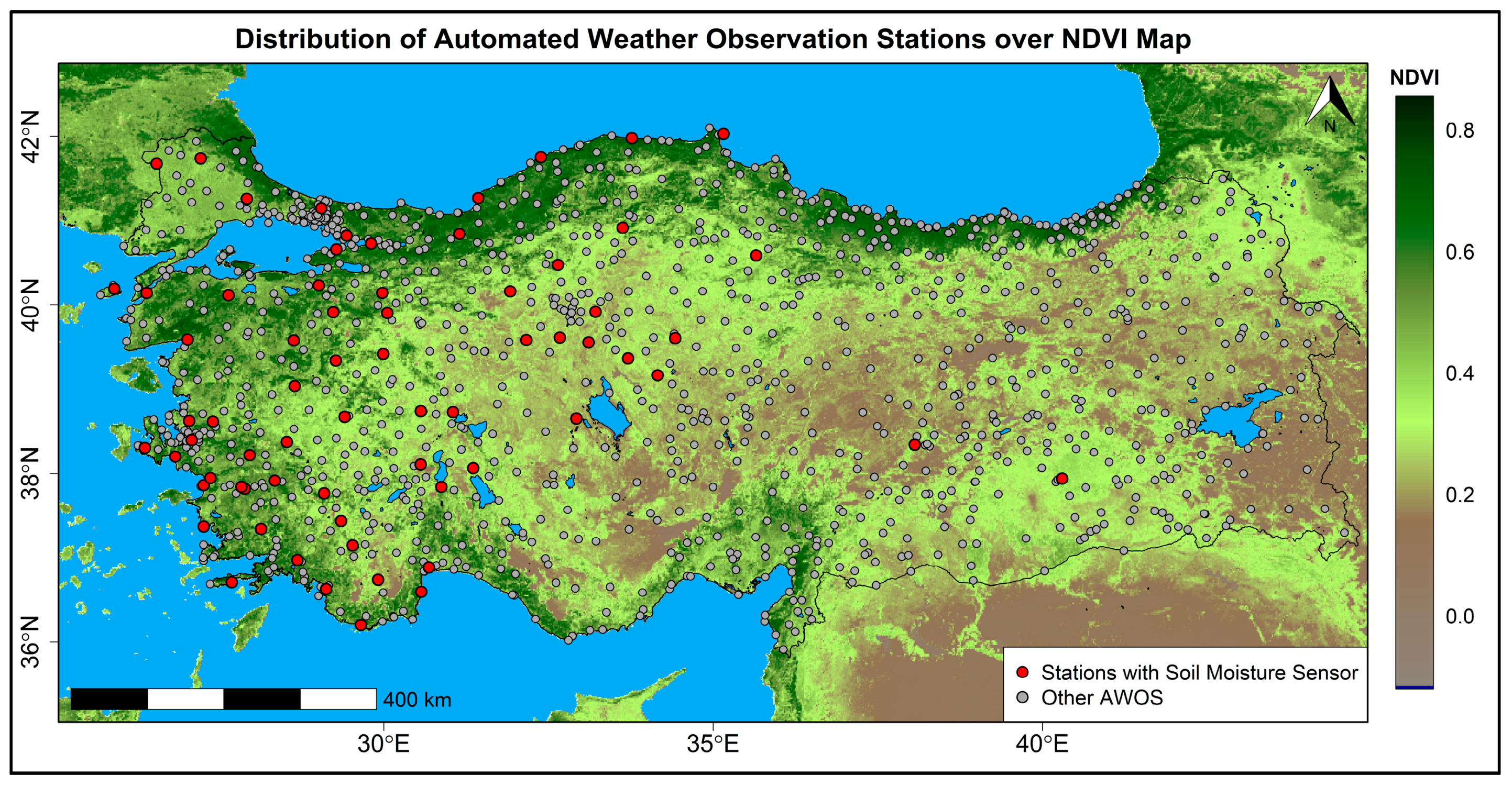
More than 1000 automated weather observation stations (AWOS) collecting hydrometeorological data (i.e., air temperature, relative humidity, wind speed and direction, precipitation, solar radiation, surface pressure, temperature, etc.) [
23,
24] are being operated in Turkey and among these some also contain soil moisture measuring sensors. These stations are part of the 206 AWOS (also called Western Mesonet) whose installations were started in 2002, and they became operational in 2007. This Western Mesonet network has been continuously expanded by new station additions since 2007 (including ongoing expansions today), bringing the current number of installed stations to more than 2000 locations. However, newly added stations do not include soil moisture sensors (but have other hydrometeorological sensors), while only some of the Western Mesonet stations have soil moisture sensors. The soil moisture observations utilized in this study are obtained from the Western Mesonet Network only. Distribution of AWOS and stations with soil moisture sensors are shown over Normalized Difference Vegetation Index (NDVI) in
Figure 1.
2.2. Station-Based Soil Moisture Measurements
The station-based soil moisture measurements are obtained using a Campbell Scientific CS616 water content reflectometer at a depth of 20 cm and 10-minute intervals. The sensor observations are based on the principle that soil and water have different electromagnetic radiation and electrical transmission properties. The sensor measures volumetric soil moisture using the dielectric constant of the soil water matrix, which is measured by utilizing the capacitance of the soil through the electromagnetic signals sent between the two parallel bars. Since the only substance that affects the transmission time of the signal sent between the two parallel bars is the water in the soil medium, the volumetric soil moisture can be measured with the help of the sensors measuring the time of the signal transmission [
25].
The CS616 and similar sensors are widely used to measure soil moisture [
26,
27]. The CS616 sensor measures the period of the signal propagation time, which is later converted to the soil moisture estimate. The soil moisture measurements made by the sensor are influenced by the type, the electrical conductivity, and the temperature of the soil. Hence, the accuracy of the observations may be improved via proper corrections/calibrations against these factors. Since the measurements are also sensitive to the temperature of the sensor, it is necessary to correct the measurements to the temperature of the soil medium utilizing the observations made at the same depth, in order to increase the accuracy of the measurements. The transformation of the measured period signal to the soil moisture values requires the use of calibration curves specific to the soil type. Accordingly, soil type dependent calibration curves are required to obtain improved soil moisture values, while the default calibration equation provided by the manufacturer reflects only a specific type of soil [
25]. This implies that the use of calibration curves specific to soil type may improve the accuracy of the retrieved soil moisture observations.
In this study, the response of the sensor according to the content of different soil types is examined, and different calibration equations are developed based on soil type or electric transmission capacity [
25].
2.2.1. Soil Type Calibration and Temperature Correction
The CS616 sensor measures the propagation time of the transmitted signal between two parallel bars. This observed periodic signal is then converted to soil moisture values using the standard Equation (1) provided in the sensor’s manual [
25].
where VWC is the volumetric water content, and τ is the period of the measured propagation time signal given in microseconds.
Here, the goal of the calibration is to obtain a separate calibration curve for each soil texture type, where soil type-specific calibration curves are expected to have fewer inversion errors (i.e., from sensor measured signals into soil moisture) than using above given default Equation (1).
Soil Texture Classification of Samples
Soil specimens collected from each station are sampled for determination of soil types using Analysis of Part Size Distribution (Sieve Analysis) and Analysis of Part Size Distribution by Sedimentation (Hydrometer). For the Sieve Analysis, the standard American Society for Testing and Materials (ASTM) D6913 [
28] is used. For this analysis, the particle size distribution is carried out by finding the proportion of particles larger than 75 μm in the soil sample. For the Hydrometer analysis, the standard ASTM D422 [
29] is used. For this analysis, the distribution of particle sizes smaller than 75 μm is determined by a sedimentation process, using a hydrometer to secure the necessary data.
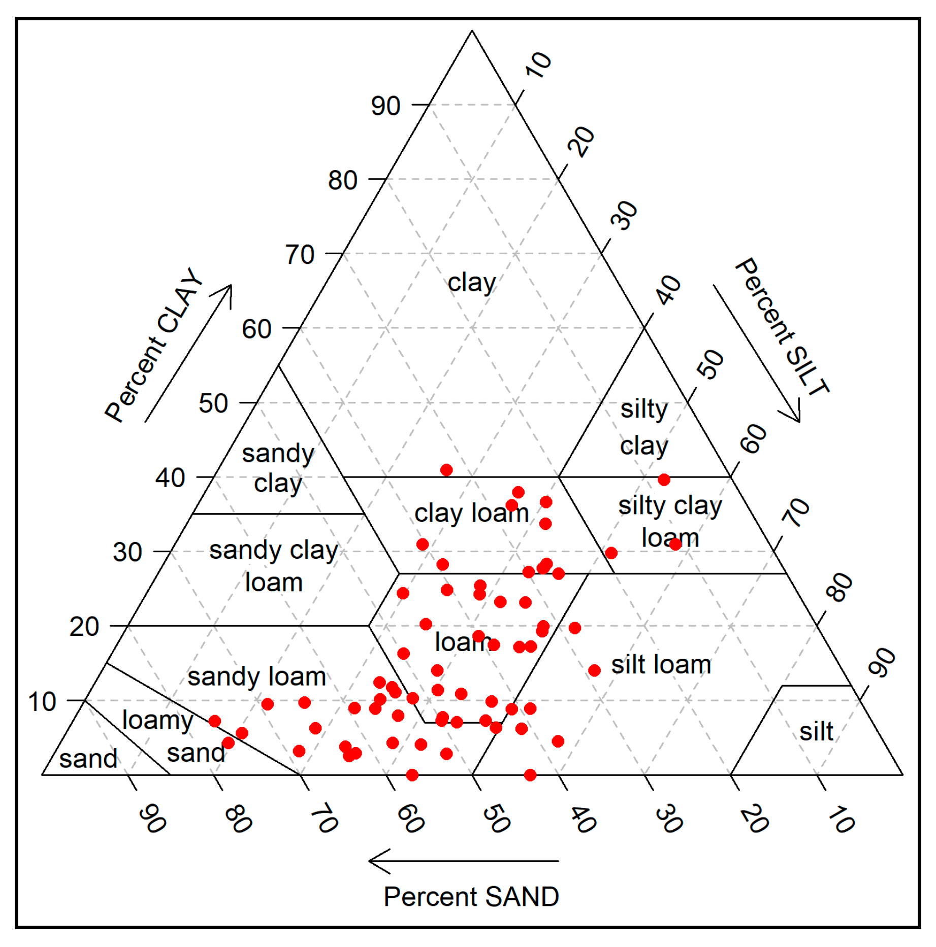
Later, the soil types of the samples are determined using the obtained soil texture ratios and the soil texture triangle given by the United State Department of Agriculture (USDA) for soil classification [
30]. The ratio of the content on each side of the triangle is marked, and the information about which type of sample this information corresponds to is obtained (
Figure 2).
Soil Type Calibration
Separate soil samples collected from different stations, all with the same soil texture, are combined into a bucket. The amount of soil from each station mixed in the bucket is the same to avoid bias from any particular station. After that, for each soil texture type, a separate bucket of soil samples is obtained. Accordingly, different soil sample groups are prepared to calculate separate calibration curves for each soil group. Soil texture types that did not have sufficient collected samples are not utilized for the calibration curve calculation; instead, default calibration curve equations provided by the manufacturer (Campbell Scientific CS616 manual [
25]) are used. Later the following procedure and the equipment used for calibration of different soil sample groups.
Procedure:
Soil samples collected from different stations with the same soil texture are mixed, while the volume of the combined samples are kept the same.
Soil samples are mixed to create a homogenous soil sample.
Soil samples are crushed with the help of the trowel before each measurement to avoid agglomeration and to acquire homogenous moisture distribution in the soil.
The soil is placed into the calibration bucket at bulk density near to field conditions.
Sensor values are read for three times.
Volumetric soil samples are collected.
The weights of the volumetric soil samples (net weight) are measured.
The calibration sample is re-wetted.
All steps are repeated until the calibration sample reaches the saturation point.
Volumetric soil samples taken at each repetition are oven-dried.
The weights of dried volumetric soil moisture samples are measured.
Equipment:
Data logger and CS616 sensor to read the measured propagation time signal period.
Cylindrical sample vessel to determine the soil moisture of the sample.
Calibration bucket (PVC, with 10 cm diameter and 35 cm length) to measure sample soil moisture using the sensor.
Sensitive scale to measure the weights of the samples.
Oven to dry the samples.
Here oven-dried samples represent the laboratory-based true soil moisture values, while sensor-based readings form the basis of sensor-based estimates. After the samples are placed into the calibration bucket, a part of the CS616 sensor—up to half of its plastic—is placed in the soil. The values are obtained via the data logger when the sensor measurements became constant. The soil medium, where the moisture is measured, is sampled with the cylindrical container; this sample is initially weighed for its wet mass and later oven-dried for 24 h to obtain the dry mass. For each group, eight measurements are made to represent eight different wetness levels. The measured period information via the CS616 sensor is then related to the actual soil moisture measurements (via oven drying) for each group separately. Later, polynomial equations, similar to Equation (1), are fitted, and the parameters that represented this best fit with minimized prediction errors are obtained. Once these soil texture dependent parameter sets are obtained for all of the six groups separately, past τ observations collected by the CS616 sensors since 2008 are converted to soil moisture values.
Correction for the Temperature
The CS616 sensor is very sensitive to the temperature of the soil medium. Calibration equations generally are obtained at a specific temperature, while the actual observations made in the field often are different. Hence, the observed period values should be initially corrected for the actual soil temperature, prior to the implementation of the calibration equations. For this reason, soil temperature observations measured at 20 cm depth (the same depth that τ observations are made) are used in temperature correction based on the CS616 sensor’s manual descriptions as follows:
where
τc is the corrected period values,
τuc are the raw uncorrected period values, and
Tsoil is the temperature of the soil medium.
2.2.2. Quality Control
Quality control is performed to ensure the reliability of the acquired soil moisture data sets. Similar to the soil temperature and the signal-period (i.e., soil moisture) observations, precipitation is also measured at the same stations every 10 minutes. The relationship between the precipitation and the signal-period observations is used to perform a visual assessment of the quality control of the period time series. Overall, the soil moisture responds to major precipitation events; any precipitation event should be followed by an increase in the signal-period, and, similarly, the absence of precipitation should yield a continuous decrease in the signal-period. If the signal-period observations do not show reasonable responses to the observed precipitation, then such observations are flagged as “bad quality” while the other observations are selected as good quality.
These quality control assessments are performed for all stations separately between 2008 and 2016 using daily values, while the sensitivity analyses (i.e., validation of remote sensing- and model-based soil moisture datasets given under
Section 2.3) are performed between 2008 and 2011. Firstly, the raw 10-minute period observations are converted to 10-minute soil moisture estimates using the default calibration Equation (1). Then, the obtained 10-minute soil moisture values are converted to daily values using the arithmetic average method. Similarly, daily-accumulated precipitation values are also calculated from 10-minute observations. Later, these daily precipitation time series are used to pre-assess the sensitivity of soil moisture time series; here, the goal is to visually examine the responses of the soil moisture sensor to the measured precipitation. An increase in the soil moisture values is expected for the periods with very high precipitation events, while a steady decrease is expected for long no-precipitation periods. In addition to the quality control of the soil moisture-precipitation relationship, the data sets are also controlled for the frozen soil conditions. The soil moisture values that are associated with the soil temperature values below 1 °C are flagged and not used in this study, as such cold conditions are assumed to contain partially or fully frozen soil medium. If the soil moisture time series obtained over any station did not consistently respond to measured precipitation data, or showed a constant value for a long period of time (i.e., no drying), or showed unexpected fluctuations (such as sudden drying), then these stations are flagged and removed from the analysis. Instead, only the soil moisture time series that showed reasonable responses to precipitation time series is used.
2.3. Validation of Remotely-sensed and Model-based Soil Moisture Products
Remote sensing-based ASCAT, AMSR-E, ESA-CCI and model-based API and NOAH soil moisture products are evaluated with station-based observations. Since AMSR-E satellite terminated its mission in October 2011 and ASCAT products are available from May 2007, the years between 2008 and 2011 are selected as the study period. Characteristics of each soil moisture source can be seen in
Table 1.
2.3.1. Remotely-sensed Soil Moisture Products
Remote sensing systems may be classified into two types depending on the incoming signal sources: (a) Radiometers are passive systems that measure the self-emission of Earth’s surface, (b) radars are active systems that measure the energy scattered back from the surface. In this study, one active (ASCAT), one passive (AMSR-E) and one combined (ESA-CCI) remotely sensed soil moisture products are used.
ASCAT
ASCAT is a real-aperture radar instrument onboard the Meteorological Operational Satellite-A (MetOp-A) satellite which measures the radar backscatter with reliable radiometric accuracy and stability [
31,
32]. The satellite was launched in October 2006 and became fully operational in May 2007. The measurement of the wind speed and direction over the oceans are the main objectives of the ASCAT, though acquired observations are also used for studying soil moisture, polar ice and vegetation. The types of electro-magnetic waves that are measured by ASCAT are VV polarization in C-band with 5.255 GHz. ASCAT observes the Earth’s surface with a varying spatial resolution of 25 km to 50 km while it reaches to 12.5 km in the higher resolution product. C-band microwaves transmitted by ASCAT have a role in measuring the soil moisture in the top 0.5 to 2 cm of the soil layer.
ASCAT product classifies the moisture in the soil between dry (0%) and wet (100%). In this study, the Technische Universität Wien (TUWIEN) soil moisture product (average of ascending and descending overpasses) that has 0.25° spatial resolution is used. The dataset used in this study is provided by the European Organization for the Exploitation of Meteorological Satellites (EUMETSAT) data center website “
https://navigator.eumetsat.int”.
AMSR-E
The instrument, which was launched in May 2002, is a dual-polarized, conical scanning, passive microwave radiometer. AMSR-E uses C-band (6.9 GHz) and X-band (10.65 and 18.7 GHz) radiance observations to derive near-surface soil moisture [
33]. Each band has different sensing depth and spatial footprint; C-band has 1–2 cm sensing depth and 74 × 43 km
2 spatial footprints while X-band has a smaller footprint and less than 5 mm penetration depths [
34]. While AMSR-E is one of the first sensors that prevalently used for the estimating soil moisture retrievals, data retrieval stopped in December 2011 when the instrument ceased operations. The products retrieved using AMSR-E observations have temporal coverage between June 2002 and October 2011.
Several algorithms have been developed to estimate soil moisture from AMSR-E retrievals [
35,
36,
37]. Although AMSR-E has several retrieval products, Land Parameter Retrievals Model (LPRM) which is the approach of Vrije Universiteit Amsterdam (VUA)–NASA, shows stronger consistency with in situ measurements in Europe [
34]. The results of LPRM model soil moisture data are available in the units of volumetric water content (m
3 m
−3) on a regular 0.25° global grid. LPRM datasets (descending overpass) used in this study are provided by NASA Goddard Space Flight Center’s Global Change Master Directory. In this study, AMSR-E abbreviation is used not only for the instrument, but also for the soil moisture product obtained by using LPRM.
ESA-CCI
ESA-CCI soil moisture product is a multi-decadal data record based on a combination of satellite observatory soil moisture datasets (both active and passive products) [
38,
39,
40]. The merging approach in the ESA CCI includes three steps. Initially, the passive microwave products are fused together; secondary, the active products are fused; and lastly, the two fused products are combined together to produce the final product.
The first version of ESA CCI (v0.1) is published in 2012. Since then, the CCI team regularly upgrade their product through expanding its time series length and spatial coverage by including new sensors, and upgrading their algorithms. In this study, the combined version of ESA CCI (v4.2) with a spatial resolution of 0.25° is obtained from ESA CCI website: “
http://www.esa-soilmoisture-cci.org”. Additional information about the ESA CCI soil moisture product and technical details of it can be found in the study of Dorigo et al. [
38].
2.3.2. Model-Based Soil Moisture Products
Similar to remote sensing-based observations, hydrological models also provide large scale soil moisture data, where the spatial resolution of the soil moisture product depends on the input forcing and ancillary datasets. In this study, soil moisture estimates retrieved from simulations of API and NOAH hydrological models are used.
NOAH
NOAH land surface model [
41] is developed by cooperative work of National Centers for Environmental Prediction (NCEP) - Oregon State University (OSU) Dept. of Atmospheric Sciences - Air Force - Hydrologic Research Lab. Like many other complex land surface models, NOAH uses atmospheric forcing data (precipitation, temperature, humidity, wind, and four-way radiation) and soil and vegetation related parameters to fully solve the energy and the water balance elements (e.g., soil moisture and soil temperature) at the land surface for specified number of soil columns and a single canopy layer. NOAH is a 1D model in the vertical direction that the solutions of energy and water balance equations are performed independently over each grid point. The model consists of one snow layer, one canopy layer, and four soil layers. Typically, four soil layers are chosen, and their depths from the ground level are typically chosen as 10 cm, 40 cm, 100 cm, and 200 cm.
The NOAH soil moisture products that are used in this study are simulated by NASA Earth Sciences Division and published by Goddard Earth Sciences (GES) Data and Information Services Center (DISC) (
http://disc.sci.gsfc.nasa.gov). The temporal resolution of the retrieved datasets are 3-h and the spatial resolution of 0.25° [
42], where the soil moisture estimates are representative for the 0–10 cm soil layer.
API
API is one of the simplest examples of hydrological models to estimate soil moisture. It calculates soil moisture using the precipitation of the region, where the retrieved soil moisture product has the same temporal and spatial resolution as the input forcing precipitation product. Several studies have been made in order to link precipitation to soil moisture by using API because of the lack of field data [
43,
44]. Because of the simplicity of its retrieval, it is much easier to have full control over synthetic experiments that investigate scientific questions theoretically and easier to infer for the moisture conditions with comparable accuracy over remote locations with limited forcing/ancillary datasets [
41,
42,
43,
44,
45]. API model-based soil moisture is calculated using the following equation:
where API
t+1 represents soil moisture values, γ is a seasonally varying parameter that determines what part of precipitation is stored in the soil, and P
t+1 is the precipitation amount observed between time t and t + 1. The γ value typically ranges between 0.85–0.98. The study of Crow et al. [
45] determined that in the sensitivity tests of API, taking γ parameter as varied rather than as a constant reveals little qualitative variation in results; hence, γ parameter is taken as constant 0.85 in this study. The errors originating from the initial value usually disappear within a short period of time [
43,
44]. In this study, API values are obtained from 2000 to the end of the study period, and the errors originating from the initial value are eliminated. As for the input precipitation data, two different products are used: Station-based precipitation observations and the Tropical Rainfall Measuring Mission 3B42 v7 (TRMM) [
46]. The TRMM dataset is obtained from NASA precipitation measurement missions’ website “
https://pmm.nasa.gov/data-access/downloads/trmm”.
2.3.3. Rescaling of Soil Moisture Datasets
Soil moisture products acquired using different platforms (i.e., station-based observations, remote sensing retrievals, hydrological model simulations) often have different vertical support (soil moisture status between 1 and 20 cm). Furthermore, these products often have different spatial and temporal representativeness characteristics in addition to their differences between the dynamics of the soil moisture values (i.e., some soil moisture values change between 0 and 0.50 while others between 0 and 1.0). All of these differences necessitate soil moisture products to be rescaled to the space of a reference dataset so that the comparisons (e.g., error statistics) can be meaningfully performed or merging algorithms could be implemented optimally.
Several linear and nonlinear rescaling methods have been proposed to rescale hydrological variables, particularly soil moisture [
47]. Among them the cumulative density function matching-based method [
48,
49,
50] is commonly used, while variance matching-based [
51,
52,
53], linear regression-based [
54,
55], Triple Collocation Analysis (TCA) based [
56], and Copula-based [
57] methods are also implemented to reduce the systematic differences between time series.
In this study, given linear regression results in the least squared errors when two datasets are regressed to each other (i.e., similar to rescaling), linear regression-based rescaling method is preferred to reduce the systematic differences that may exist between soil moisture time series [
56] obtained from station observations, satellite retrievals, and hydrological model estimates.
Overall, linear rescaling methods are implemented by considering the most general linear relation between a reference dataset X and the dataset to be rescaled Y in the form
where Y* is the rescaled version of Y,
and
are time-averages of X and Y, and
is a scalar rescaling factor. Here
in this study is found using regression-based linear methods as
where
is a linear rescaling factor;
and
are standard deviations of X and Y datasets, respectively; and
is the correlation coefficient between X and Y. Here in these equations X and Y datasets refer to station-based observations and evaluated soil moisture products (e.g., remote sensing- or model-based), respectively.
2.3.4. Validation Statistics
In this study, evaluations of soil moisture products are performed using the Pearson correlation coefficient (R), and root mean square error (RMSE) following Entekhabi et al. [
58]. Here these statistics are calculated after products are linearly rescaled to station-based observation space using Equations (4) and (5):
where N is size of the sample, μ is mean value,
and
are the standard deviations of X and Y, respectively, and
is Pearson correlation between X, Y, and Y* values are the rescaled products (remotely-sensed or model-based). Here, RMSE can also be equally called error standard deviation or unbiased root mean square error given product X is selected as the truth and Y is the evaluated product, while the differences between the means of X and Y are removed via Equation (4) given above.
2.3.5. Evaluation Categories
Validation of remote sensing- and hydrological model-based soil moisture products with station observations are performed over each station separately. The analyses are further expanded by investigation of the error statistics for (1) seasonality/anomaly components, (2) different soil types, (3) climate regions and (4) vegetation cover.
The soil moisture time series are decomposed into their seasonality (i.e., low frequency) and anomaly (i.e., high frequency) components for further investigations. Most of the drought studies discarded the seasonality and made drought analysis based on soil moisture anomaly data [
2,
59]. In addition, triple collocation-derived error data is calculated over anomaly values [
60,
61]. For this reason, it is important to evaluate seasonality and the anomaly components of the different soil moisture product separately. In this study, the seasonality components are calculated by taking the 29-day moving window average for each day-of-year (i.e., total 365) using the datasets obtained from all years (i.e., average of 29*5=145 soil moisture values obtained from 14 days before and after for the day-of-interest using all 4 years between 2008 and 2011) [
21]:
where X
d is seasonality value for day-of-year d, SM is the soil moisture value for any day of any year. Once the daily seasonality components are calculated, the daily anomaly components are calculated by subtracting seasonality values from daily soil moisture value.
With a separate calibration curve is obtained for each soil category (e.g., sand, silt, clay), the effect of soil type on the accuracy of the satellite- and model-based products are calculated by investigation of the statistics over different soil type categories.
The variability of the climate across Turkey is large, hence, different climate zones [
62] obtained from Köppen-Geiger Climate classification [
63] are often used to investigate the impact of the climate as a part of sensitivity studies.
Vegetation cover is another issue to be taken into consideration while evaluating the performance of different soil moisture products. Since vegetation cover affects the remote sensing-based and model-based soil moisture products, the average NDVI values (MODIS/Terra Vegetation Indices Monthly L3 Global 0.05-degree) in the study period are used to obtain vegetation cover of each station. The NDVI dataset used in this study was obtained from the MODIS web site “
https://modis.gsfc.nasa.gov/data/dataprod/mod13.php”.
3. Results
3.1. Temperature Correction, Calibration, and Quality Control
Soil texture classification (i.e., ratios) results for five stations with different soil types are shown in
Table 2. Following the ASTM standard, the particles which passed sieve No.200 (75-μm) are considered as silt and clay; particles which could not pass sieve No.4 (4.75 mm) are considered as gravel. The rest of the particles which remained between the two sieves are considered as sand. The silt ratio is obtained by subtracting the clay ratio (obtained by hydrometer test) from particles passed No.200 sieve.
As an example, for the soil sample taken from station #17024 Kastamonu İnebolu, the sand, silt, and clay ratios are 26.51%, 46.47%, and 27.03%, respectively (after the gravel ratio is subtracted). When these ratios are marked in the USDA soil texture triangle, the soil class is then found to be “clay loam”. The same procedure is repeated for all stations, and the soil classifications are obtained for all samples (
Figure 2). Sieve analysis and soil texture analysis results show that loam and sandy loam soil classes are the most common soil types among the analyzed samples (
Table 3).
For each group, eight measurements representing different soil wetness are made. The difference between the dry and the wet soil sample mass, in addition to the sample cylinder volume (~2750 cm
3) information, enabled the actual volumetric soil moisture of the soil groups to be calculated. As an example, the actual and the estimated (via CS616 sensor) soil moisture values for Group 4 are given in
Table 4.
Here the actual soil moisture values range between 7.69% and 55.61%, while the error standard deviations for the estimates obtained using the manufacturer-provided default and calibrated equations are 3.66% and 2.75% respectively for Group 4. As expected, the errors of the estimates using calibrated equations are consistently lower than estimates using default equations on both the dry and the wet edges, showing soil-type calibration consistently improves the soil moisture estimates.
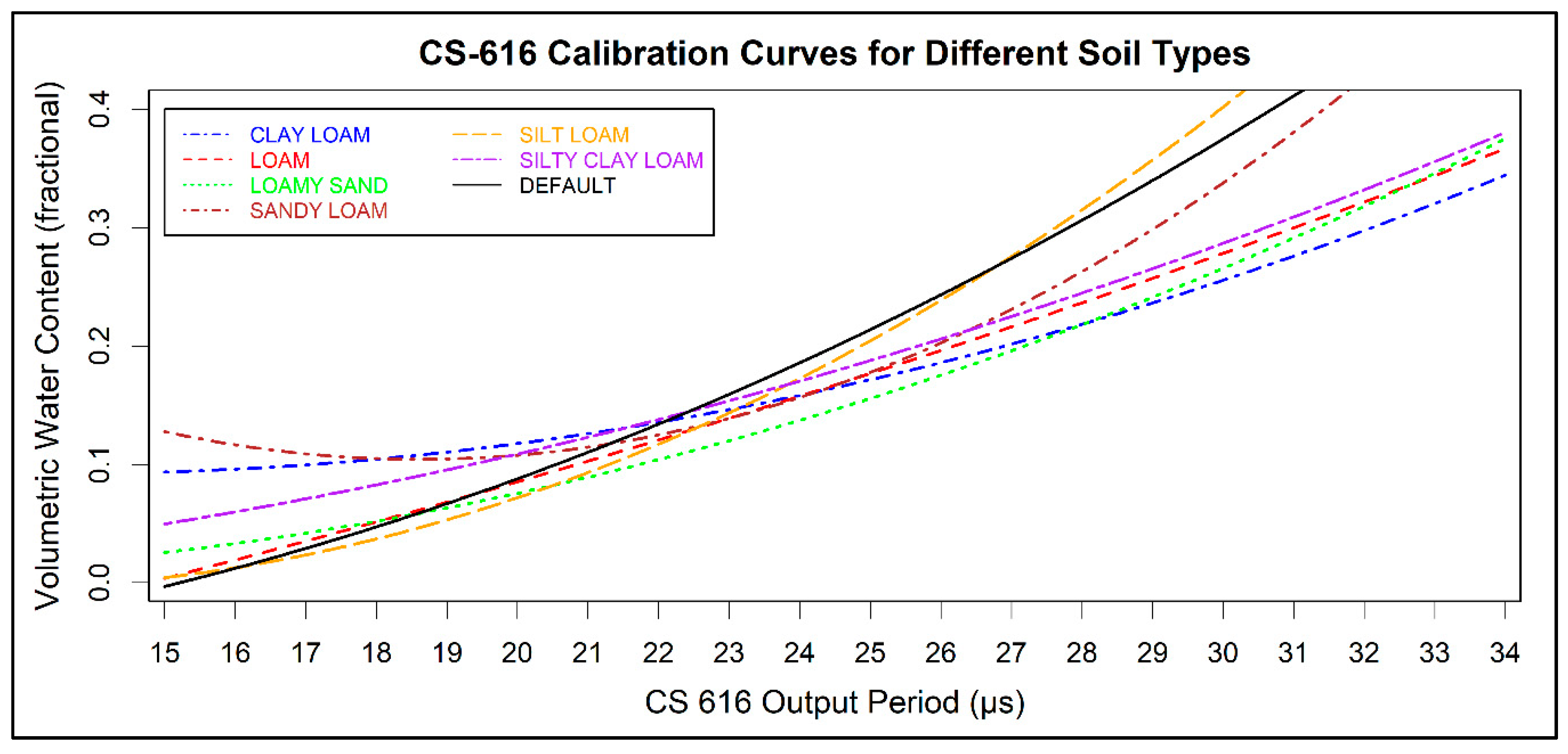
In addition to the actual soil moisture measurements, CS616 sensor-based period measurements are also made for the same soil groups, under the same conditions that the actual soil moisture measurements are made. The CS616 sensor period measurements for each of the six soil groups are related to actual soil moisture observations using polynomial equations (
Figure 3) that yield the lowest root mean squared errors (RMSE). These soil texture type-specific polynomial equations are later used to convert signal period observations into volumetric soil moisture values.
The ensemble of calibration curves found for different soil groups greatly vary from the default calibration curve provided by the manufacturer, except for silt loam (
Figure 3); this group had a similar curve to the default curve. These curves are later applied to convert the temperature corrected period information to sensor-based soil moisture readings. The difference between the actual soil moisture and the sensor readings is considered the sensor measurement error.
The error statistics of the soil moisture values retrieved using the default and the calibrated equations, found in this study, are given in
Table 5. On average, the calibration removed the bias and the RMSE effectively for most of the soil types. The standard deviation of the soil moisture reading errors are, on average, 3.0%, and varied between 2.0% and 3.4%. These results show that the CS616 manual accuracy estimate of 2.5% is lower than the 3.02% standard deviation results found in this study.
As an example, for the calibrated sensor-based soil moisture estimates, the time series for station number 17746 is shown in
Figure 3. The soil moisture readings respond to the precipitation with increased soil moisture values and show a steady and gradual decrease during the dry period without precipitation. The increase in the soil moisture values after a precipitation event is much higher after a long dry period than after a relatively wet period, showing expected soil moisture sensor sensitivity (
Figure 4).
Soil moisture time series obtained using soil texture specific curves are later quality controlled for their consistency in time and against precipitation dataset variability. Here the goal of this quality control is to eliminate the time series without consistent/continuous soil moisture signal via visual inspection of the soil moisture time series. After these rigorous quality control steps, time series obtained over 68 stations are selected and used in this study (
Table A1 and
Figure 1), while other station-based sensor readings (i.e., time series) are flagged and removed from the analysis. The most common reason for the elimination of time series is found to be the lack of sensor reading sensitivity to precipitation; an increase during wet periods or continuous decrease during dry periods is not observed. The number of eliminated time series having very high soil moisture values (>60%) or unrealistically changing soil moisture variability (e.g., for several years the soil moisture standard deviation is 0.10 while the following years it is 0.005) was less than 10.
3.2. Validation
Satellite- and model-based soil moisture estimates are validated using the CS616-based soil moisture observations as the truth. These validation analyses include the calculation of correlation coefficient and RMSE over each station separately. Because the satellite and the model datasets have different soil moisture space, they are first rescaled to the space of CS616 sensor-based soil moisture using linear regression before the error statistics are calculated. The satellite and the model soil moisture data over each station are extracted using selecting the data of the pixel that contains the station coordinates. The datasets for the stations that have mutually available soil moisture products (total 40 stations) are used in a separate analysis to make an objective evaluation of the product accuracies. Here, mutual availability refers to the stations that have partial/full temporal coverage for all products over each location, while the statistics are not calculated using temporally mutually available days (the number of temporally mutually available days is very low), but rather the statistics are calculated using all available data over each station separately. Other individual statistics are also given to evaluate the performance of different soil moisture products over Turkey. Overall, the validation analyses are investigated for all stations together and for stations split into different classes with respect to annual mean soil moisture, climate, and soil type.
3.2.1. Validation—All Stations
The correlation and RMSE results of different soil moisture products are calculated over all available stations and mutually available stations, while average error statistics for both cases are given in
Table 6. Error statistics are calculated for the complete time series, the seasonality component (and the anomaly component separately using Equation (7). Confidence intervals of error statistics for the complete time series at a 5% significance level (CI
95) are calculated using the bootstrap method with thousand samples (n = 1000).
On average, the seasonality component has a much higher linear correlation with the ground-based datasets when compared to the linear correlation of the complete and the anomaly datasets. Here, the averaged seasonality component correlations are as high as 0.95 (for NOAH) while the averaged anomaly component correlations are as low as 0.28 (for AMSR-E). Original time series of NOAH soil moisture product gives the highest correlation (R = 0.82) with station observations; yet, on average, the anomaly component of API-Station has a much higher correlation (R = 0.63) than the correlation of the anomaly components of NOAH (R = 0.50) and API-TRMM (R = 0.46). This result shows the significance of accurate precipitation forcing datasets, and soil moisture anomaly components of NOAH simulations still have room for improvement using more accurate precipitation forcing. In general, the remote sensing-based products have fewer anomaly correlations than the model anomaly components. Among remotely-sensed products, ESA-CCI soil moisture product has the highest correlation in all three components (Com. R = 0.71, Season. R = 0.92, Anom. R = 0.42), implying the most consistent product among the ones evaluated in this study. The results of RMSE show on average the products have around or lower than 0.040 m
3 m
−3 error; implying the validation goal of remotely sensed soil moisture products (i.e., accuracy requirement of 0.040 m
3 m
−3 RMSE for more recent soil moisture missions SMOS, SMAP and products of The Global Observing System for Climate (GCOS) [
10,
18,
64]) is satisfied over the stations used in this study (even the requirement is not valid for AMSR-E and ASCAT). When the anomaly and the seasonality components are investigated separately, the errors become less than 0.03 and around 0.03, respectively; while the NOAH seasonality component errors become as low as 0.012. Such low seasonality errors are the primary reason why NOAH complete time series has very high correlations against the sensor-based observations. Overall, average error statistics obtained using all station datasets are not considerably different from error statistics obtained using only mutually available station datasets. This similarity is perhaps because the number of mutually available stations (40) is high enough compared against the total number of available stations (between 44 and 67). Accordingly, from this point, only the analyses conducted using mutually available station datasets will be discussed.
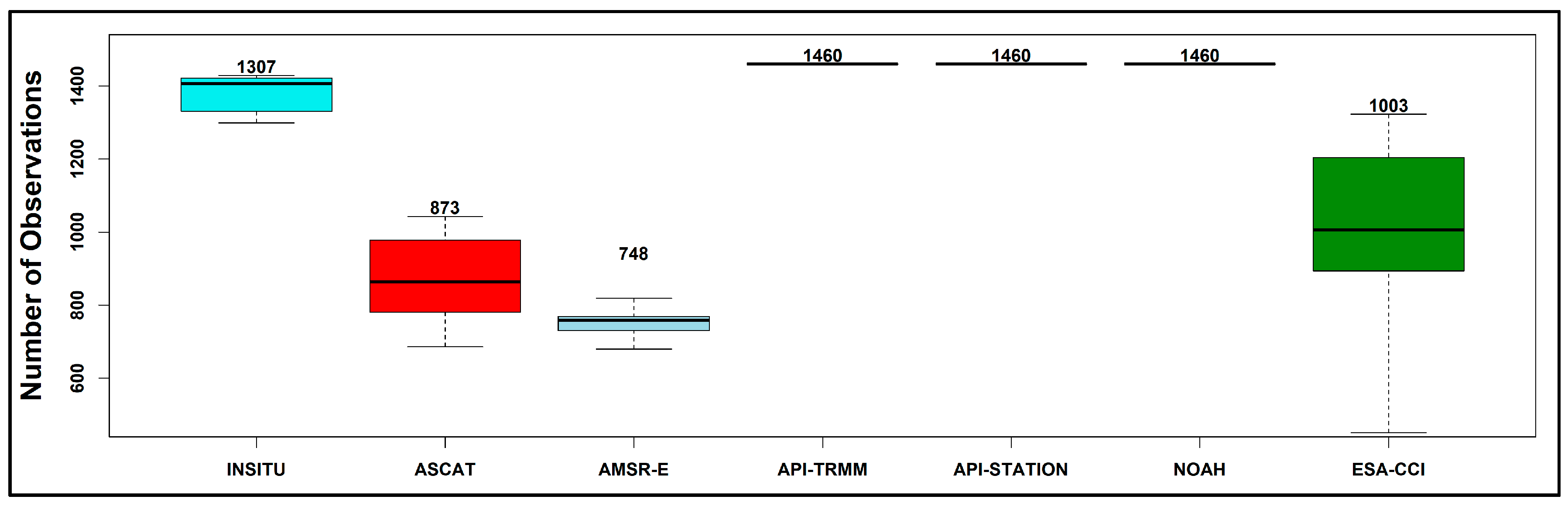
The temporal data availability of each soil moisture product over 40 stations (i.e., the datasets are mutually available) is shown in
Figure 5 (numbers over the boxes show mean values). As expected, model-based soil moisture products can be obtained during the entire study period (i.e., 1460 days between 2008 and 2011). On average, both the mean and the variability of ESA-CCI’s temporal data availability is higher than those of other two remotely-sensed products. The advantage of ESA-CCI in this temporal availability stems from the fact that it is a combined product of multiple datasets; if one of the parent datasets is missing, then the other parent dataset(s) provides the data. AMSR-E soil moisture data has the lowest temporal coverage over mutually available stations with a mean value of 748 days.
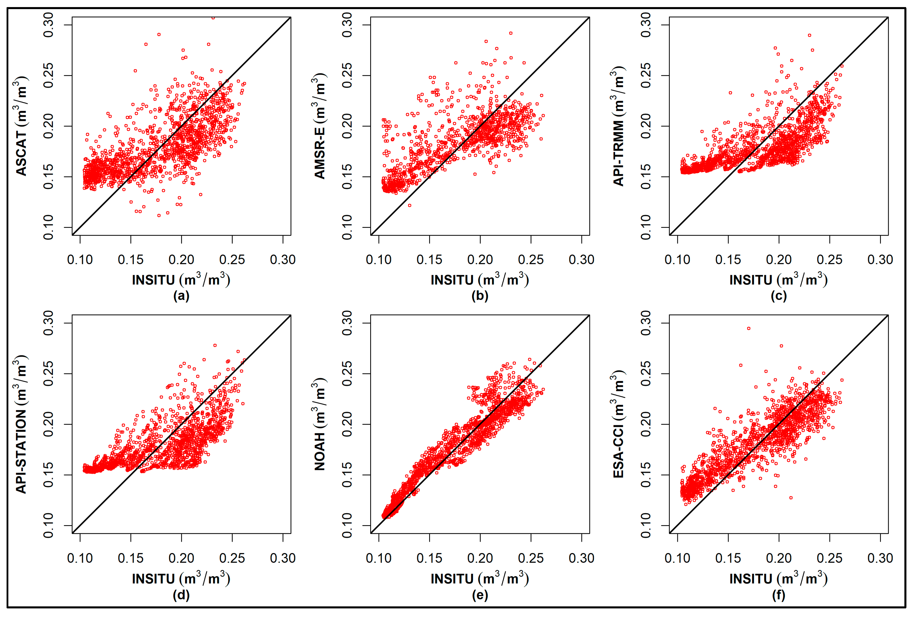
Figure 6 shows the scatter plot of each soil moisture product over mutually available stations (the soil moisture values are spatially-averaged over 40 stations to obtain a single time series).
The favorable error statistics of NOAH and ESA-CCI (
Table 5) are confirmed over these scatter plots that NOAH and ESA-CCI time series have much better consistency (i.e., deviations from 1:1 line is the least) with the station-based observations than other products. While other products particularly suffer around the dry edge of the scatter (i.e., persistent overestimation), NOAH and ESA-CCI have much better performance for low values. While this result is partially stemming from the selected rescaling methodology (i.e., linear regression), it is also impacted by the high accuracy nature of these datasets. Saturation of API soil moisture product around 0.16 is a direct result of the fact that the original unscaled product saturates around 0 which is originated from the simple Equation (3) that is used to convert precipitation values to soil moisture values while the rescaling methodology brings these 0 values to 0.16. Overall, ASCAT and AMSR-E also show a good relationship with station-based observations.
3.2.2. Validation—Categories
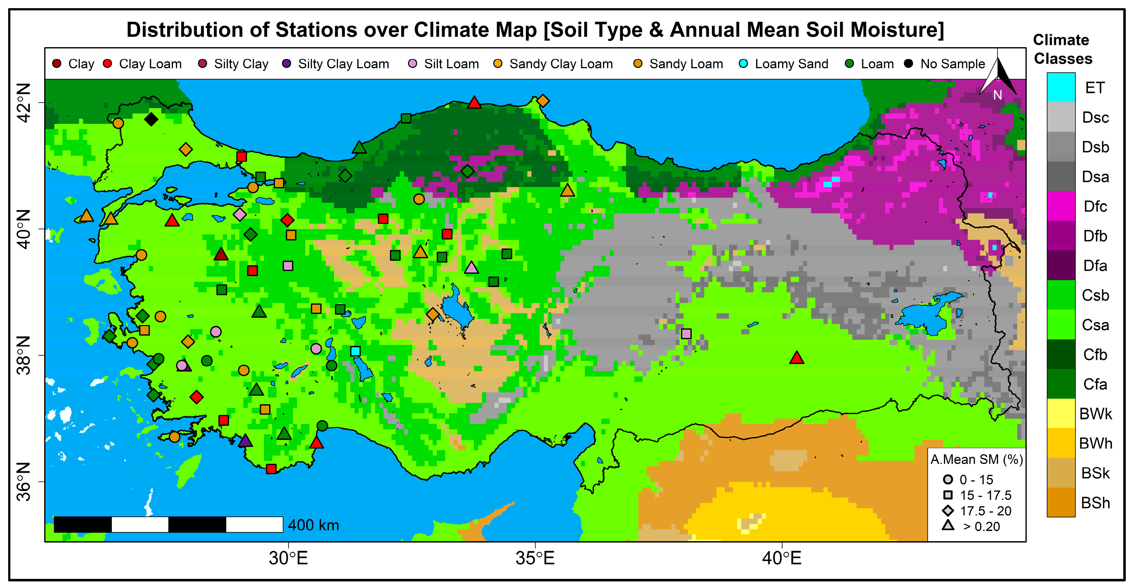
The information about stations related to selected analysis categories (soil type, climate and annual mean soil moisture) is given in
Figure 7.
The soil type of the station is shown by the specific color, annual mean soil moisture range of the station is given by the specific shape, and map colors show the climate classes (i.e., the figure contains three legends for the soil type, the climate, the average soil moisture). Annual mean soil moisture thresholds are selected to ensure four wetness sub-class have, approximately, the same number of stations in each sub-class. Similar to annual mean soil moisture, mean NDVI thresholds are also selected to ensure, approximately, the same number of stations in each sub-class. Even though more complex terrains exist over eastern Turkey, the stations are located over relatively less-complex regions in the western parts of Turkey. In general, the sub-classes are not dominated by any particular sub-class (e.g., Csb climate sub-class have different soil types (colors) and average soil moisture values (shapes)).
The categorical correlations and RMSE of each product for the annual mean soil moisture are shown in
Figure 8 and
Figure 9, the climate regime is shown in
Figure 10 and
Figure 11, the soil type is shown in
Figure 12 and
Figure 13, and the mean NDVI (vegetation cover) is shown in
Figure 14 and
Figure 15. Each category is further divided into four different sub-classes to the sensitivity of the soil moisture product accuracies to the variability in the sub-classes. While the total number of stations used for each category is the same (40 stations except soil type category), each sub-class category has a different number of stations (given at the top of each sub-class).
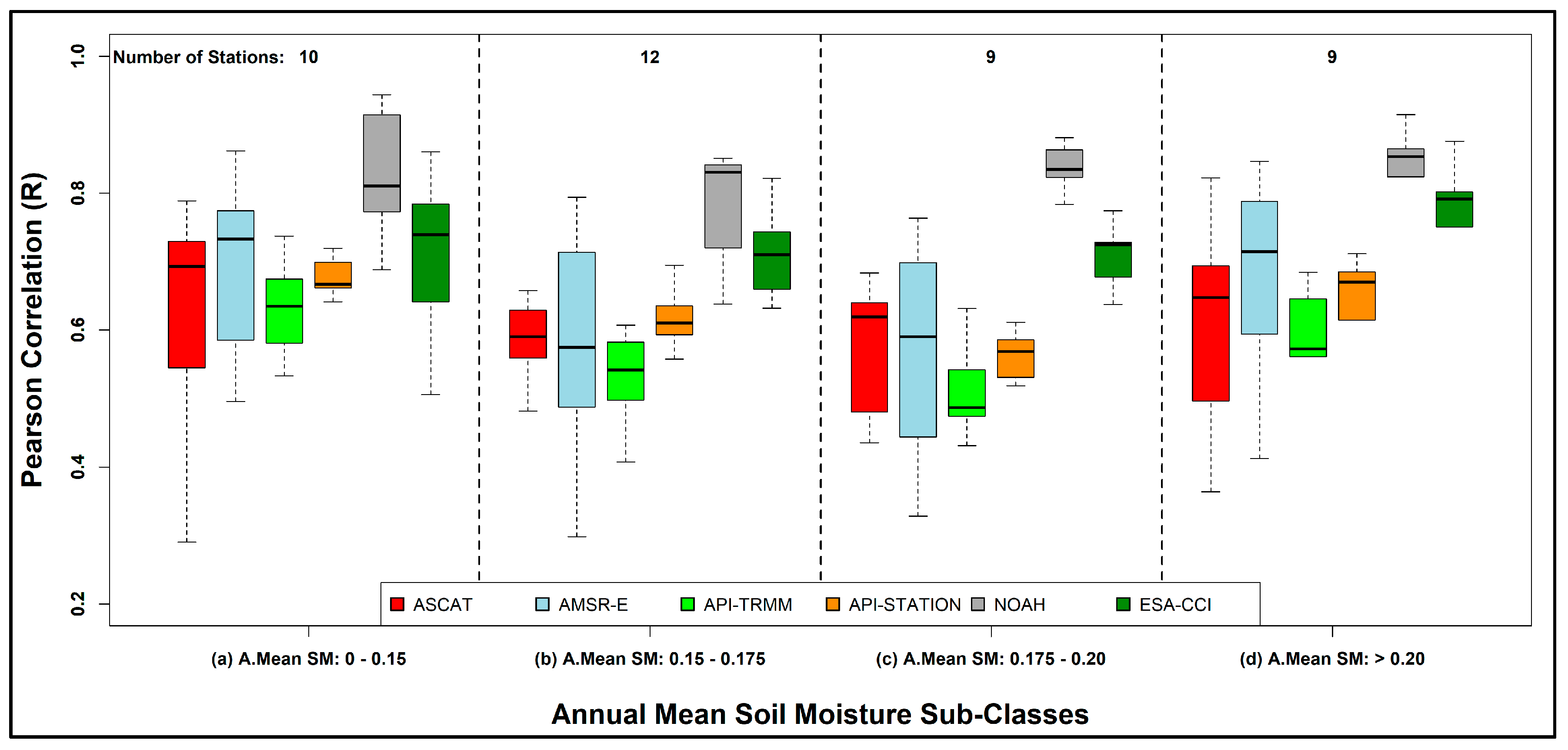
The variability of the correlation and RMSE statistics classified with respect to the annual mean soil moisture sub-classes are shown in
Figure 8 and
Figure 9, respectively.
Here the interval thresholds (i.e., 0.15, 0.175, and 0.20) are determined for the purpose of having a similar number of stations in each sub-class. Overall, NOAH and ESA-CCI correlation variations are decreased when the wetness level is increased (consistency increases). On average, the spread of the correlations of AMSR-E and ASCAT soil moisture products are relatively higher than all other products at all sub-classes. In general, it is not possible to determine an increase or decrease in correlations with increasing/decreasing wetness; implying the product correlations are not sensitive to the mean soil moisture values over the 40 stations investigated.
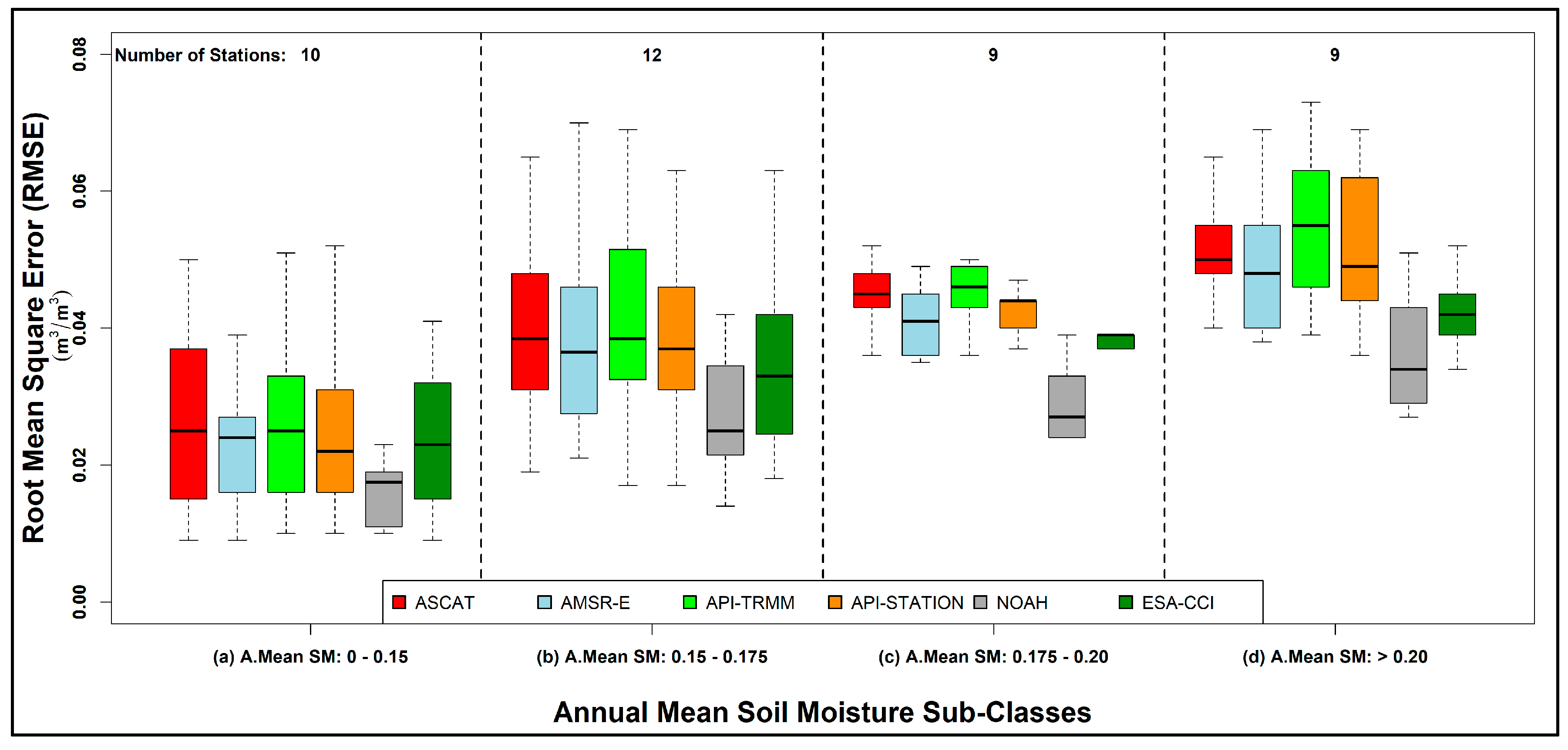
On the other hand, RMSE values clearly increase with increasing soil moisture values (
Figure 9); this implies the increasing errors are due to the increased variability of the products where the ratio of the error variance and total variance (i.e., inherently related to the correlation coefficient) remains similar. The variation of RMSE values is relatively lower in sub-class 3 compared to other sub-classes (
Figure 9c). Except for the AMSR-E, ASCAT, and API estimates at the wet sub-classes (
Figure 9c–d) only, all soil moisture products in all sub-classes have less than 0.04 m
3 m
−3 RMSE. ESA-CCI product relative performance compared to other products (except for NOAH) becomes better with increasing soil moisture (
Figure 9). Overall, the NOAH product has the least error in all sub-classes.
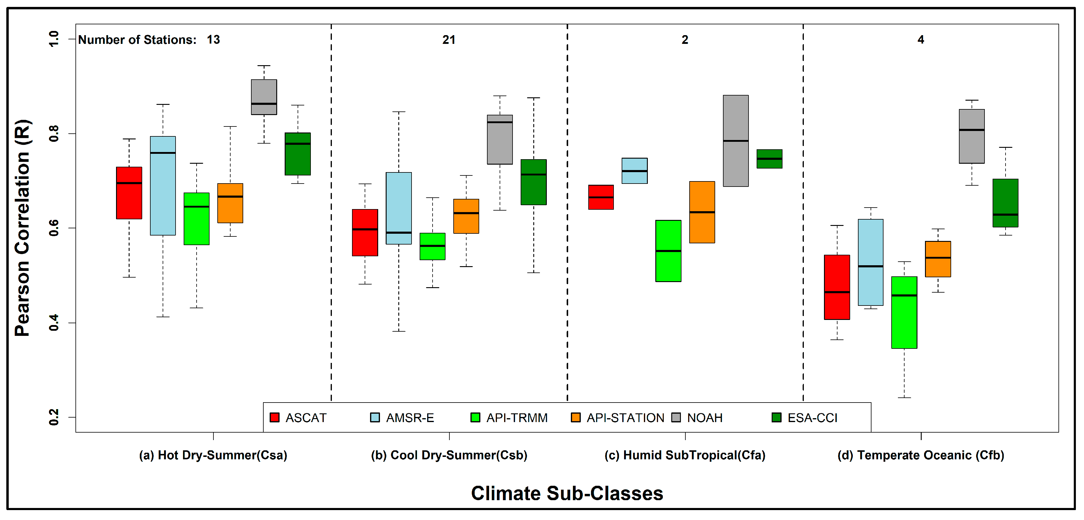
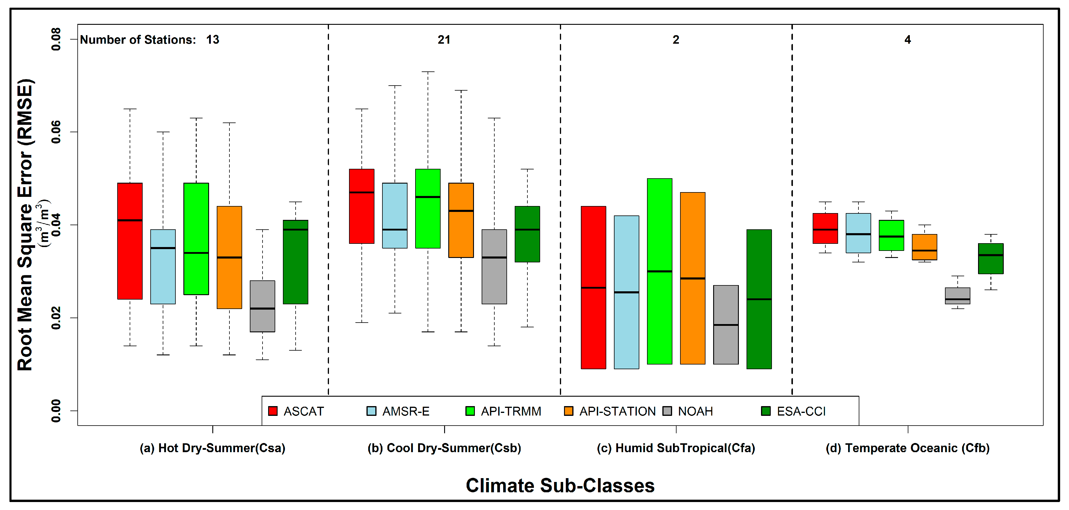
The variability of the correlation and RMSE statistics classified with respect to the climate sub-classes are shown in
Figure 10 and
Figure 11, respectively.
Here, the climate sub-classes are obtained by using Köppen-Geiger Climate Classification and the heavy majority of the stations are classified under the Hot-Dry Summer Csa (
Figure 9a) and Cool-Dry Summer Csb (
Figure 9b) classes. Correlations calculated over hot-dry summer (Csa) stations are relatively higher than other sub-classes for all soil moisture products, while in temperate oceanic sub-class (Cfb), correlation of all products is slightly lower than other sub-classes. On the other hand, Cfb sub-class has the lowest uncertainty of the box plot quartiles. Parallel to the correlation results (
Figure 10), RMSE values also indicate similar relative accuracy estimates for each climate regime sub-class (i.e., higher correlations follow lower RMSE, and vice versa). All products have higher errors over cool dry-summer conditions while compared with all other sub-classes.
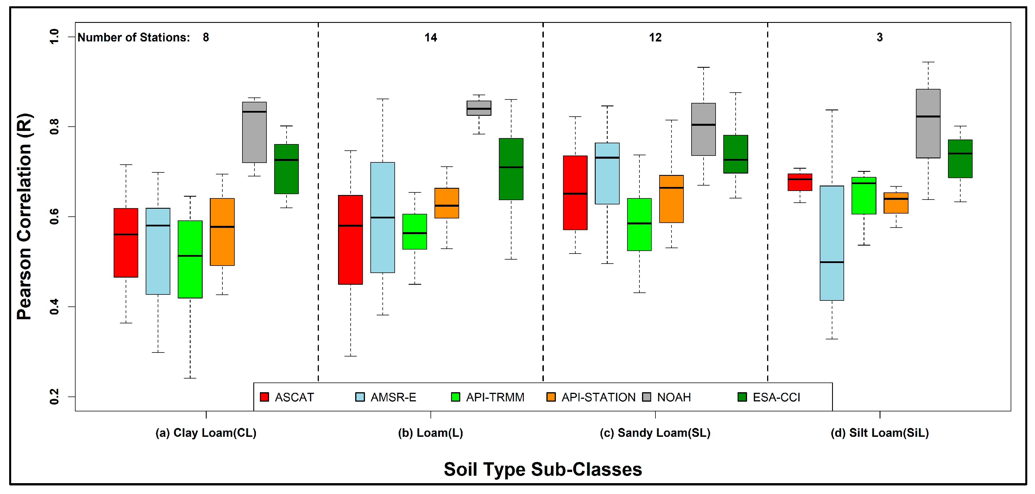
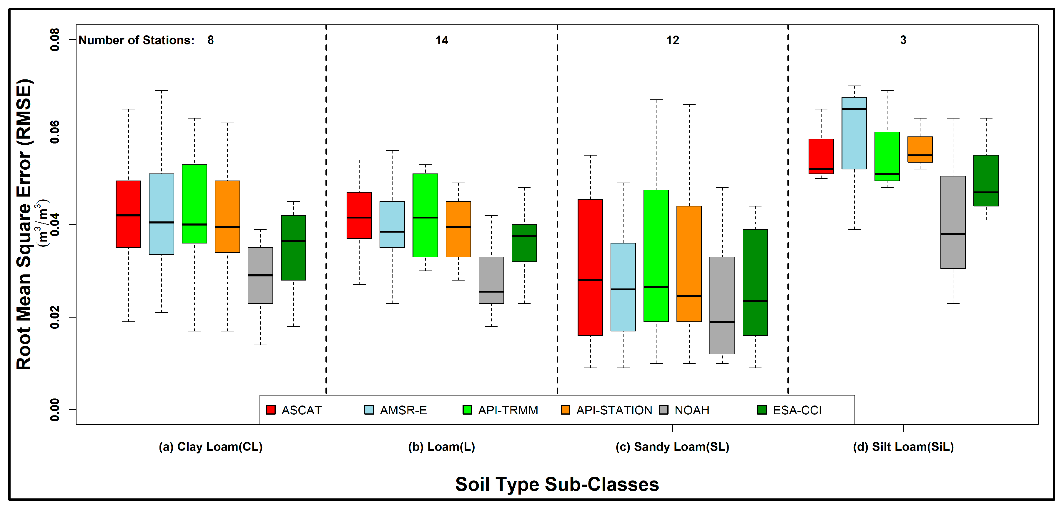
The variability of the correlation and RMSE statistics classified with respect to the soil type sub-classes are shown in
Figure 12 and
Figure 13, respectively.
In clay loam sub-class (
Figure 12a), correlations of NOAH and ESA-CCI products are significantly higher than other products with respect to the other sub-classes, while the difference is reduced in sandy loam sub-class. On average, the correlations of ASCAT, AMSR-E, and API products show a slightly increasing correlation pattern from clay loam to loam and then to sandy loam. Similar to other analysis categories, in this category, NOAH product shows the highest consistency (lowest errors) with station observations in all soil sub-classes. However, in sandy loam sub-class (
Figure 13c) RMSE values show the highest variation even though on average, the lowest mean RMSE values are obtained for all products compared with other soil types. The highest RMSE values are found in silt loam soil type for all products, while the number of stations used for this soil type is the lowest (i.e., sampling errors are highest).
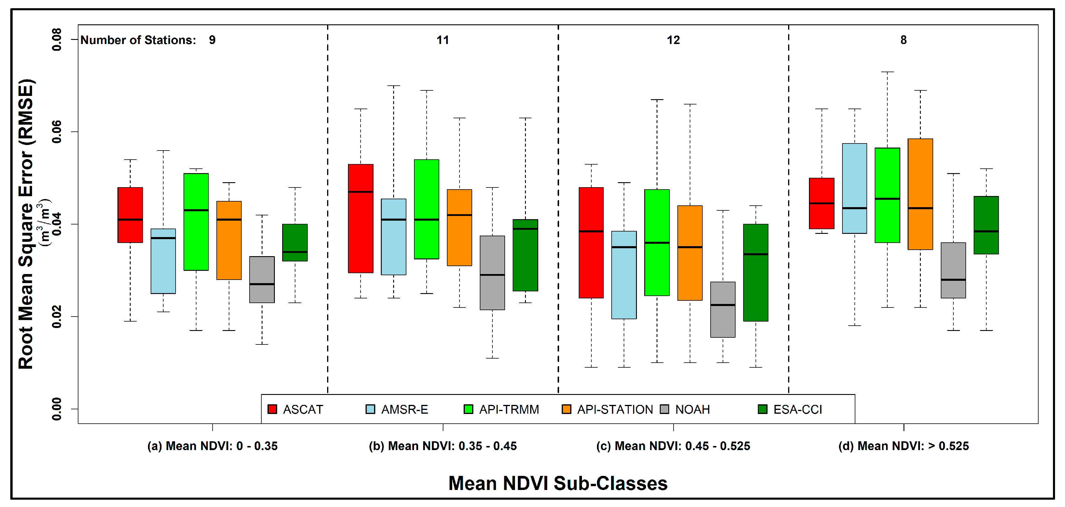
The variability of the correlation and RMSE statistics classified with respect to the mean NDVI sub-classes are shown in
Figure 14 and
Figure 15, respectively.
Here the interval thresholds (i.e., 0.35, 0.45, and 0.525) are determined for the purpose of having a similar number of stations in each sub-class. Overall, in the first three sub-classes (
Figure 14a–c) an increase in correlation values of all products is observed, on the other hand, in the densest vegetation cover sub-class (
Figure 14d) all products show lower correlation values and the highest variation in correlation. Effects of vegetation cover on NOAH and ESA-CCI soil moisture products are fewer than other products, while the correlation values of these two products is nearly the same in all sub-classes. Correlation variation of AMSR-E soil moisture product is found to be higher compared to all the other products in their respective sub-classes. In
Figure 15, RMSE values in the densest sub-class are higher for all soil moisture products. Similar to correlation results, RMSE results also showed that NOAH and ESA-CCI soil moisture products are affected by vegetation cover less than other products.
Due to the selection thresholds of sub-classes, even though the mean NDVI values get denser, a decrease in correlation and an increase in RMSE are not observed. However, the lowest correlation values and the highest RMSE values relative to the other sub-classes for all products, are found in the densest sub-class (
Figure 14 and
Figure 15d).
4. Discussion
In this study, apart from the validation of 6 different soil moisture products using station-based observations, the accuracy of sensors used in stations and possible factors that may affect the performance of products are also considered. The analyses are elaborated by classifying the stations for their soil type, climate regime and annual mean soil moisture value to investigate the sensitivity of the soil moisture values against these classifications.
Manufacturer manual stated accuracy estimate of CS616 sensors is ±2.5% VWC; however, in this study, the errors are found as 3.0%. The study of Varble et al. [
15] determined the similar accuracy results for CS616 sensors. Overall, the accuracy estimates for the calibrated sensors vary for different soil types (the RMSE for Loam is 2.35%, and for Clay Loam it is close to remote sensing-based satellite mission requirements of 4.11%). This study could be repeated using the same sensors over different locations to reach a more general statement about the CS616 sensor accuracy and its relation with different soil type.
In general, the SMOS, SMAP satellite missions and terrestrial essential climate variables product requirements [
10,
18,
64] (0.04 m
3 m
−3) (even the requirement is not valid for AMSR-E and ASCAT) are for the entire time series, while the most relevant information about the soil moisture for most applications is for their anomaly components. This is particularly true for the drought-related soil moisture applications. Given the anomaly and the seasonality components of soil moisture products have different accuracies, perhaps the mission requirements should be updated considering these different components. Similarly, the RMSE values are sensitive to the average wetness of the soil; hence, mission requirements should perhaps indicate wetness level along with the requirement statistics. Overall, if the validation results obtained using drier-region-observations are, on average, expected to yield smaller RMSE results than using wetter-region-observations. Here, selection of a dimensionless accuracy statistic (e.g., correlation coefficient) may partially eliminate the impact of soil wetness deviations over the accuracy (i.e., the correlation accuracy estimates are much less sensitive to RMSE accuracy estimates in
Figure 8 and
Figure 9).
The accuracy statistics obtained using all datasets and only the time series that are mutually available for all products do not differ; this shows the accuracy of the missing time series for different products are not relatively more or less accurate than the mutually available stations. Perhaps, the analysis of mutually available station selection might not be necessary next to the statistics obtained using all available datasets, particularly the number of stations is relatively high.
NOAH and ESA-CCI product accuracies are the highest among the model and the remote sensing products used in this study. Nevertheless, these high accuracies imply the merging of these two datasets (perhaps in a data assimilation framework) might yield a more accurate product. Overall, API values do not have as much sensitivity to soil moisture at low values, perhaps as a result of its simplistic modeling approach (Equation (3)) which only relies on the precipitation as input forcing and do not use other hydrometeorological variables (i.e., drying rate is not a function of other variables like temperature). On the other hand, API values (particularly when high accuracy station-based precipitation forcing dataset is used) have high anomaly component accuracy relative to other products, implying a high potential in applications requiring anomaly information (e.g., drought).
API-station yields the best anomaly accuracy (also better than API-TRMM). This result particularly shows the significance of station-based precipitation products and the added errors via precipitation inputs in the hydrological models. This implies, if more accurate (i.e., station-based) precipitation products could be used as input in the NOAH hydrological model rather than global datasets like TRMM, then it is viable that much better soil moisture anomaly estimates could be obtained in addition to the already highly accurate NOAH seasonality estimates.
AMSR-E soil moisture product was observed to be more sensitive to vegetation cover relative to other remote sensed based products ASCAT and ESA-CCI, since its correlation values slightly decreased over stations with dense vegetation. ASCAT’s better performance compared to AMSR-E soil moisture products in the evaluation category of dense vegetation cover (mean NDVI > 0.525) might be explained by the added utility of the active (scatterometer) sensors compared against the passive (radiometer) sensors that ASCAT soil moisture product was also found as less effected by vegetation than AMSR-E product in previous studies [
6,
65].
In this study, the errors over silt loam soil type are much higher than other sub-classes, while on average lower errors are found over sandy loam soil type. While this difference may indicate the sensitivity of products to the soil type, it also plausible that this difference might stem from higher sampling errors as the number of stations in this group is only three. Hence, the analysis of remotely sensed soil moisture products according to soil type should be repeated among different soil moisture networks. If the specific soil type-related errors occur in other networks, perhaps the soil type may be added to the retrieval algorithm. Furthermore, if the validation results in different soil types are different, perhaps comparisons may need to be made separately according to soil types, and validation studies from different stations should take this into account.
In addition, since both the NOAH model [
65] and the AMSR-E LPRM algorithm [
66] use soil texture as an input parameter, comparing Food and Agriculture Organization (FAO) soil texture and laboratory results is beneficial before evaluating how soil types affect both of the soil moisture products. For this reason, FAO soil texture is obtained at each station, and the statistics and comparison to laboratory results are given in
Table 7. On average, the variability of station-based soil texture estimations (i.e., sand, silt, and clay fractions) are considerably less for FAO than the variability of ground measurements, even though their mean values are similar. The difference between the FAO and ground estimates could be due to the spatial representativeness errors of ground measurements or due to the FAO estimates coarse spatial resolution may poorly reflect the ground conditions. In either case, these differences contribute as additional error source to NOAH and AMSR-E soil moisture products.
The anomaly component (i.e., primarily used in many drought-related studies) correlations of models are much lower than the seasonality component accuracy for different products, while the use of station-based precipitation as forcing improves the simple API model accuracy by 0.15 (
Table 6). Even though the NOAH model is not run using identical conditions with varying precipitation forcing, the use of much higher accuracy precipitation forcing might considerably improve the NOAH soil moisture results.
Overall, when the NOAH and the ESA-CCI wetness increases, then the variability of the obtained correlations against the station-based observations decreases. This implies the signal-to-noise ratio of these products and the sensitivity to soil moisture increase as the soil moisture increases.
5. Conclusions
In this study, sensitivity of the accuracy of ASCAT, AMSR-E, ESA-CCI, API, and NOAH soil moisture products to soil type (silt, clay, and loam ratios), climate regime, and time series components (i.e., seasonality and anomaly components) using ground station-based observations obtained over Turkey between January 2008 and December 2011. Raw station-based observations are later post-processed (quality control, soil temperature-based correction, and soil texture type-based calibration of soil moisture time series obtained from 68 stations). For the soil type-based calibration, the texture information is obtained via analysis using the soil samples, while visual quality control is separately performed for each time series using observed precipitation values. Different numbers of stations are used to investigate the performance of each product separately, while mutually available station datasets are used to make an objective accuracy inter-comparison in an additional separate analysis.
Overall, the error estimates given in the manual of the CS616 sensors are found to be less than the error estimates found in this study. The soil moisture time series that passed the rigorous quality control steps performed in this study had signals consistent with precipitation events and showed the expected sensitivity.
NOAH soil moisture time series yield the best agreement (over mutually available stations; R = 0.82 and RMSE = 0.028 m3 m−3) with station-based measurements and among remotely-sensed products, ESA-CCI product gives the best performance (R = 0.71 and RMSE = 0.034 m3 m−3). Seasonality is determined as the dominant component of soil moisture time series for all products with higher correlations values respect to anomaly component. In addition, in terms of anomaly components, the API-Station product showed the best overall performance among all sites.
Here in this study, the soil moisture products are evaluated based on ancillary information about the stations, like soil type, vegetation cover, climate region and the wetness. Overall, the climate-based classification did not show much variability in the accuracy statistics; model- and remote sensing-based products accuracies seemed to be less sensitive to the climate classifications selected in this study. On the other hand, vegetation cover and the soil wetness of the study area have a much higher impact over the variability of the product accuracies. The climate and the wetness-based selections are not as much coupled in this study, and that is why the climate and wetness-based results differ.
This study is expected to increase the use of these datasets as this soil moisture network contains many stations located over complex topography, while the number of such station-based soil moisture estimates is very limited. Moreover, the compared and validated remotely-sensed and model-based soil moisture products in this study could be used according to evaluated categories in future works related to soil moisture. However, more studies are needed to generalize the statements obtained in this study, as only 68 station-based datasets are used in this study.

 ,
, 


