Detecting Vegetation Variations and Main Drivers over the Agropastoral Ecotone of Northern China through the Ensemble Empirical Mode Decomposition Method

Abstract

Vegetation is the major component of the terrestrial ecosystem. Understanding both climate change and anthropogenically induced vegetation variation is essential for ecosystem management. In this study, we used an ensemble empirical mode decomposition (EEMD) method and a linear regression model to investigate spatiotemporal variations in the normalized difference vegetation index (NDVI) over the agropastoral ecotone of northern China (APENC) during the 1982–2015 period. A quantitative approach was proposed based on the residual trend (RESTREND) method to distinguish the effects of climatic (i.e., temperature (TEM), precipitation (PRE), total downward solar radiation (RAD), and near surface wind speed (SWS)) and anthropogenic effects on vegetation variations. The results showed that the NDVI exhibited a significant greening trend of 0.002 year⁻¹ over the entire study period of 1982–2015 and that areas with monotonous greening dominated the entire APENC, occupying 40.97% of the region. A browning trend was also found in the central and northern parts of the APENC. PRE presented the highest spatial correlation with the NDVI and climate factors, suggesting that PRE was the most important factor affecting NDVI changes in the study area. In addition, the RESTREND results indicated that anthropogenic contributions dominated the vegetation variations in the APENC. Therefore, reusing farmland for grass and tree planting made a positive contribution to vegetation restoration, while deforestation, overgrazing, and the reclamation of grasslands were the opposite. In addition, with the continuous implementation of national ecological engineering programs such as the Grain to Green Program, positive human activity contributions to vegetation greening significantly increased. These results will support decision- and policy-making in the assessment and rehabilitation of ecosystems in the study region.

1. Introduction

Agropastoral ecotones (hereafter APEs) refer to transition zones interlaced by croplands and grasslands [1], and they are widely distributed in the arid and semiarid regions of the world [2]. In China, the APEs area spans throughout the whole mainland from northeast to southwest, covering 13.35% of China’s land area (1.29 million km²), with residential populations and grain yield accounting for 4.68% (59.30 million) and 7.98% of the total population and grain yield of China, respectively [3]. Therefore, the arid and semiarid agropastoral ecotone of northern China (hereafter APENC) is a typical ecologically transitional zone (largest in area and the longest in spatial scale), which effectively prevents the desert in the northwest from spreading south and east [4]. Therefore, the APENC is a crucial ecological barrier for ecological security and a primary area for social and economic development in China. However, due to the effects of climate and anthropogenic factors, ecosystems have suffered different degrees of degradation in the APENC. Vegetation, as the major component of the terrestrial ecosystem [5], plays a crucial role in linking the atmosphere, hydrosphere, and pedosphere [6]. Vegetation also serves as a sensitive indicator of an ecosystem’s status and could reflect regional ecological security [7,8]. Therefore, systematic monitoring of vegetation dynamics and quantitative analyses of factors affecting vegetation variations at spatiotemporal scales are essential to understand the sustainability of terrestrial ecosystems, especially in areas with fragile ecosystems and high sensitivity to external environmental changes.

Remote sensing technology provides continuous spatiotemporal observation datasets for detecting vegetation variation at a large scale [9]. As an important remote sensing product, the normalized difference vegetation index (NDVI) is strongly linked with fractional vegetation cover (FVC), biophysical properties, biomass, and photosynthesis intensity, and the NDVI has been extensively used as an indicator of vegetation density, health, net primary production, and growth dynamics [10,11,12]. Reliable gridded NDVI products from regional to global scales are essential for the accurate modeling of terrestrial vegetation states over broad scales. The Global Inventory Monitoring and Modeling Study (GIMMS) NDVI dataset has been proven to be a long-term remote sensing measurement of terrestrial ecosystems and has been successfully applied to quantify vegetation activity and monitor vegetation dynamics in many biomes at home and abroad [13,14,15]. In the context of climate change, with increasing anthropogenic activities and a high sensitivity of vegetation dynamics to environmental changes, analyzing the temporal trend with the NDVI has proven to be particularly useful for characterizing the response of vegetation to external phenomena over a range of time scales [16].

Effective methodology development for multitemporal data analysis is one of the most vital and complicated issues in the remote sensing community [17]. In addition to the traditional linear regression method, nonlinear fitting methods have been regarded as a new way to analyze vegetation dynamics, including Fourier analysis [18], wavelet-based methods [19], breaks for additive season and trend (BFAST) [20], and detecting breakpoints and estimating segments in trend (DBEST) [16]. Although these tools were developed to detect changes in the vegetation variation trend, Fourier analysis mainly focuses on annual fluctuation, and the dataset to be analyzed should be absolutely periodic or stationary [21]; wavelet analysis is sensitive to noise; and trend detection methods are limited by the linear and nonlinear assumptions of signals [22]. Meanwhile, BFAST analysis predigests nonlinear trend components into some trend sections [23], and the intrinsic trend cannot be expressed; and DBEST analyses are more sensitive to trend changes with short durations, such as trend changes induced by wildfires and recovery [24]. However, as an improvement to empirical mode decomposition (EMD), the ensemble empirical mode decomposition (EEMD) method provides a new way to examine time series [25]. Compared to the traditional methods, the main advantages of EEMD are self-adaptive, with strong physical space and frequency space abilities at a very local scale [26]. EEMD can separate intrinsic time trend and frequency components from a signal sequence, especially nonlinear and nonstationary signal sequences [25,27]. Therefore, EEMD, as an innovative statistical tool, has been widely used to determine the time series trend in variables across various fields, such as signal and image processing, economics, health, environment, and climate determinations [28,29,30,31]. Recently, EEMD has been applied to the remote sensing field [32,33].

An accurate description of the vegetation variation is the premise for understanding the influence of climate factors and anthropogenic activities on vegetation variation. Meanwhile, identifying vegetation drives, separating anthropogenic-driven vegetation variations from climate-induced vegetation changes, and quantifying the positive and negative effects of anthropogenic activities are important bases for preserving ecosystem services and evaluating vegetation restoration policies.

Over the last few decades, to protect ecosystems from further degradation, many ecological restoration policies have been implemented in the APENC, particularly since 2000. The predominant restoration projects in this region are the “Grain for Green” program, which returns grazing land to grasslands, and the Beijing–Tianjin Sandstorm Source Control Project [34,35]. As mentioned above, the state of vegetation in this region is not only related to local ecosystem services and human welfare, but also has an important impact on the environment in northern China. Previous studies have used line regression methods to investigate vegetation variations and related effects of climate and anthropogenic activity [8,36]. However, limitations in the vegetation change trend detection method have hindered our ability to investigate the drivers of vegetation variations [37,38]. Therefore, evaluating vegetation variations using nonlinear methods may help us obtain a deeper understanding of vegetation variations and their correlations with climate change and anthropogenic activities. Thus, the main objectives of this study were to (a) analyze the spatiotemporal vegetation variations in the APENC, (b) identify different vegetation variation trends, (c) separate human-driven from climatically induced vegetation changes, and (d) quantify the positive and negative effects of anthropogenic activity on vegetation variation. In the context of recent pressure from human activities on vegetation, this approach is particularly beneficial for decision-making on land use management and ecological restoration policies.

2. Materials and Methods

2.1. Study Area Description

The study was conducted across the agropastoral ecotone in northern China (APENC), which lies between 100°51′–124°35′E and 35°3′–47°39′N with a general elevation of 72–4,781 m above sea level and has an area of approximately 0.62 million km² (Figure 1). The region is mainly located in the southeastern Inner Mongolia Plateau and the northern Loess Plateau. The APENC is a climate and ecological transition belt, with a semiarid temperate steppe dominated by animal husbandry to the north and a subhumid agricultural plain region to the south that connects the farmland and pastoral areas. The main land use includes grassland, cropland, desert, and forest. The climate of the area is characterized by a transition zone from semiarid to subhumid, with an annual average temperature of approximately 6.0 to 8.5 °C and an annual precipitation ranging from 150 mm in the north to 600 mm in the south. Furthermore, the precipitation is seasonally uneven and mainly occurs during summer in the form of high-intensity rainstorms from July to September, accounting for approximately 60%–70% of the annual precipitation.

2.2. Datasets

2.2.1. Global Inventory Modeling and Mapping Studies (GIMMS) Data

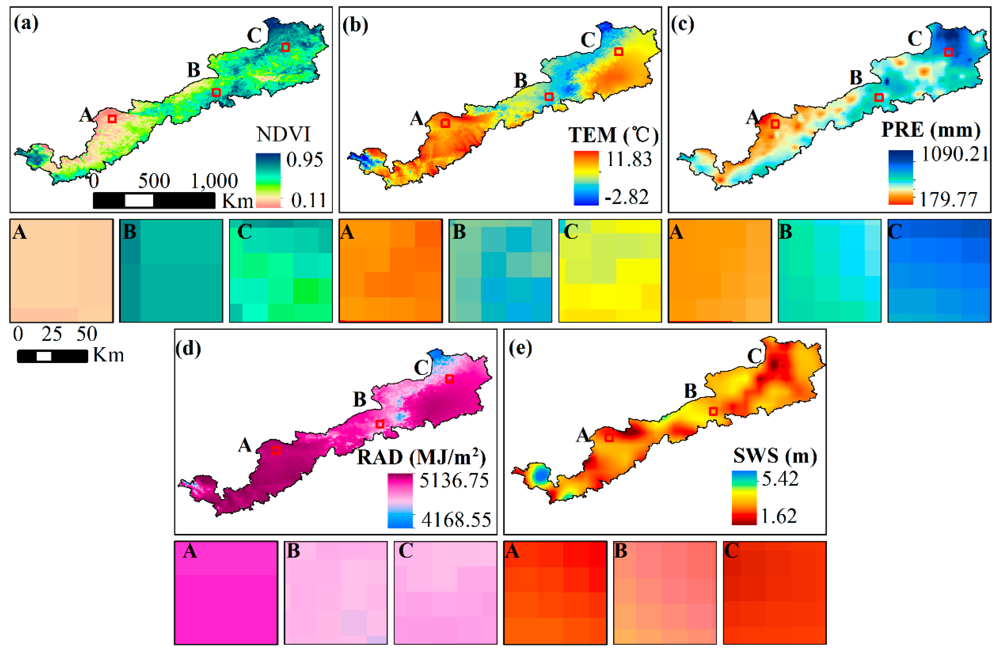
The third generation of NDVI datasets, which were derived from the Global Inventory Modeling and Mapping Studies (GIMMS NDVI3g) (https://ecocast.arc.nasa.gov/data/pub/gimms/3g.v1/) and span from 1982 to 2015, were applied to study vegetation variations over the entire APENC. The dataset is a new long-term time series version, with a spatial resolution of 1/12° and a temporal resolution of 15 days. Yearly NDVI values were calculated through the maximum value composite (MVC) method, which minimizes the influence of clouds, sun angle, water vapor, aerosols, and directional surface reflectance on the NDVI image [39]. To better match the gridded meteorological data, the GIMMS NDVI data were upscaled to 0.1° × 0.1° resolution using the bilinear interpolation method in ArcGIS 10.3, and the data sample from 2015 is shown in Figure 2.

2.2.2. Climatic Datasets

Climatic datasets, including air temperature, cumulative precipitation, downward shortwave and longwave radiation, and near-surface 10-m wind speed were collected from the China Meteorological Forcing Dataset (CMFD). The entire climate dataset spans from 1979 to 2015, with a temporal resolution of 3 h and a spatial resolution of 0.1° [40]. Previous studies have proven that climatic data from CMFD agree with observation data [41,42]. In this study, the annual precipitation (PRE), average temperature (TEM), near-surface wind speed (SWS), and total downward solar radiation, including shortwave and longwave (RAD), from 1982 to 2015 were used to analyze the correlation between the NDVI and climate factors. The four climate data samples from 2015 are shown in Figure 2.

2.2.3. Land Use and Land Cover (LUCC) Dataset

The land use and land cover (LUCC) data (1980, 2000, and 2015) used in this study from the Resources and Environmental Data Cloud Platform (http://www.resdc.cn/data.aspx?DATAID=99) [43]. The LUCC dataset was gridded with a 1-km resolution and contains 6 primary land use types, including grasslands, croplands, forests, water bodies, construction lands, and deserts, and 25 secondary land use types are also included. Grasslands are the most widespread land use type in the APENC. To further analyze the land use changes, grassland types with different coverages at the secondary level were used in this study, including high-coverage grasslands, medium-coverage grasslands, and low-coverage grasslands. Finally, eight land cover types, i.e., croplands, forests, water bodies, construction lands, deserts, high-coverage grasslands, medium-coverage grasslands, and low-coverage grasslands, were selected. Notably, considering the time coherence between the different types of datasets in our study, the LUCC data in 1980 were used to substitute the LUCC in 1982 data since such data were not available. Land use and land cover type conversion between 1982 and 2000 and 2000 and 2015 are shown in Figure 3.

2.3. Methods

2.3.1. Ensemble Empirical Mode Decomposition (EEMD) Method

The EEMD originated from the EMD [44], which is capable of extracting the secular variation trend via the removal of different frequency components from a signal sequence. Overall, the EMD is a dyadic filter capable of separating the time series signal x(t) into different kinds of time series components known as intrinsic mode functions ((IMFs); IMF i = 1…n), and the procedure continues until the residue term R(t) is less than a predetermined value of consequence or the residue term R(t) becomes a monotonic function (Equation (7)) [21]. Then, the signal x(t) is finally expressed as the sum of the (IMF i = 1…n) components plus the final residue term R(t).

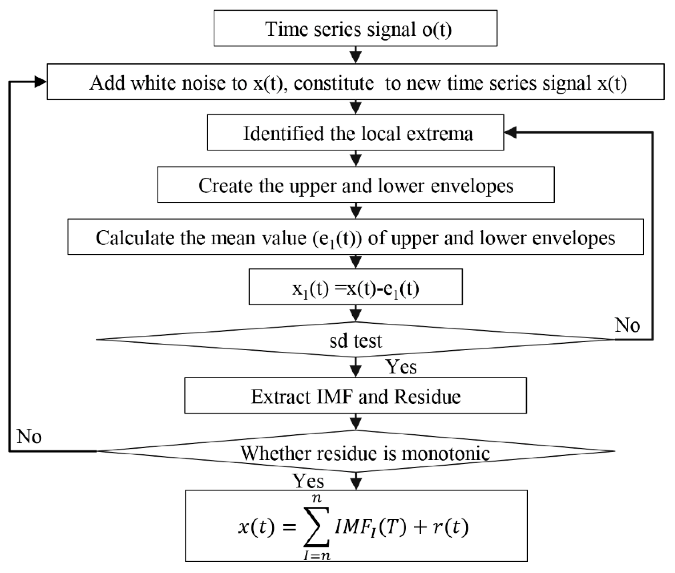
However, mode mixing is the obvious defect of the EMD, which implies a single IMF subsisting off other signals from dissimilar scales or a signal of the same scale appearing in divergent IMF components [44]. To overcome the problem of mode mixing in the EMD method, Wu and Huang [25] designed a new noise-assisted signal analysis technique called EEMD, which efficiently improved the mode mixing problem in EMD and preserved the ability of binary filters. The main point of the improved EEMD method is to add white noise to the time series signal x(t) sequence. Through EEMD decomposition, the added white noise can be cancelled out, and the signal x(t) can be decomposed into the IMFs and residue term R(t). The residual term (Rn) is considered to have detached fluctuant components and reserved secular trends, and it represents the intrinsic signal trend. Generally, the Rn is monotonic or contains an extreme value, which is identified as the turning point at the extremum. A flow chart of the proposed method is illustrated in Figure 4, and the decomposition process can be described as follows:

Step 1. Add a number of white noise q(t) to original signal o(t) [25]:

$$x\left(t\right)=o\left(t\right)+q\left(t\right);$$

(1)

Step 2. Identify the local extrema of new signal x₁(t), use cubic spline interpolation to create the upper and lower envelopes, and calculate the mean value e₁(t) of the upper and lower envelopes [21]:

$$x_1\left(t\right)=x\left(t\right)-e_1\left(t\right);$$

(2)

Step 3. Use standard deviation (sd) to determine whether the above process is to be continued or stop sifting [21]:

$$\mathrm{sd}={\sum }_{t=0}^t\left[{\left|x_i\left(t\right)-x_{\left(i-1\right)}\left(t\right)\right|}^2/x_{\left(i-1\right)}^2\left(t\right)\right],$$

(3)

where i is the number of iterations;

Step 4. When the sd is smaller than a pregiven value, the above process should be stopped, and the first IMF1 is calculated [21]:

$$\mathrm{IMF}1=x_t\left(t\right)=x_{t-1}\left(t\right)-e_t\left(t\right);$$

(4)

Step 5. The rest data r(t) are the differences between IMF1 and signal x₁(t) [21]:

$$r\left(t\right)=x\left(t\right)-\mathrm{IMF}1;$$

(5)

Step 6. Repeat step 1 to step 5 until r_n(t) becomes a monotonic function [21]:

$$r_i=r_{i-1}-{IMF}_i,i=2,3\dots n;$$

(6)

Step 7. Thus, the number of IMFs and a residual separated from x(t) [21] are obtained:

$$x\left(t\right)={\sum }_{i=1}^n{IMF}_i\left(t\right)+r\left(t\right).$$

(7)

In this study, when the EEMD method was applied to analyze the NDVI series, a total of 100 Gaussian white noise series were added to the signal sequence, with an amplitude of 0.2 standard deviations from the signal sequence. Subsequently, the NDVI trend at each pixel was obtained based on the EEMD method, and the accumulated trend was represented as the increment of the NDVI trend compared to the initial time in 1982 (Equation (8)) [45], while the instantaneous trend was regarded as the interannual variation in the NDVI trend (Equation (9)) [45] and the significance test was verified according to Pan’s method [9]. In addition, we also calculated the tendencies of TEM, PRE, RAD, and SWS over the entire study period:

$${Trend}_{EEMD}\left(t\right)=R_n\left(t\right)-R_n\left(t_0\right),$$

(8)

$${Trend}_{inst}\left(t\right)=R_n\left(t\right)-R_n\left(t-1\right),$$

(9)

where t is the end time of the study period (e.g., t = 2015), and t₀ is the beginning time of the study period (e.g., t₀ = 1982).

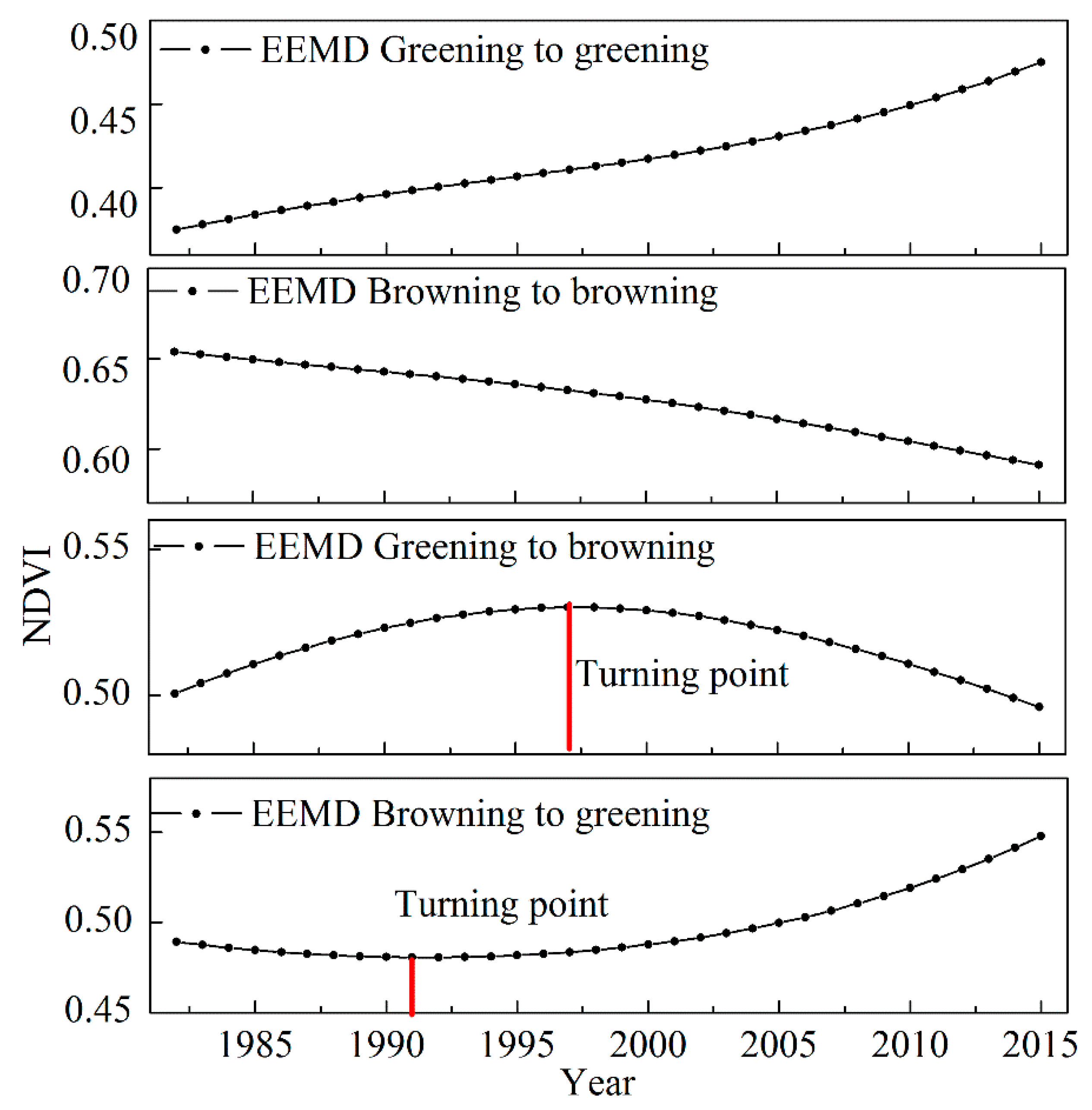
According to the Rn trend of each NDVI series, the EEMD trends in the NDVI could be classified into five classes. When the NDVI showed a significant monotonic upward or downward trend (P < 0.05), the trend was considered to be monotonic greening or browning. When the trend contained one extreme point and at least one year passed the significance test (P < 0.05), the NDVI trend was classified into greening to browning or browning to greening classes. However, if there was no significant change in the NDVI variation trend, it was classified as no significant change. Four pixels were randomly selected from the NDVI dataset of the APENC as samples of the NDVI variation trend, and they are shown in Figure 5.

2.3.2. Linear Regression Analysis

The least squares method based on a linear regression was used to investigate the change rate of the NDVI at a pixel scale [46]:

$${Slope}_{NDVI}=\frac{n{\sum }_{t=1}^{n}t\times {NDVI}_t-{\sum }_{t=1}^{n}t{\sum }_{t=1}^n{NDVI}_t}{n{\sum }_{t=1}^n{t}^2-{\left({\sum }_{t=1}^{n}t\right)}^2},$$

(10)

where${Slope}_{NDVI}$ is the NDVI change rate; t is the year order from 1 to n; n is the number of years; and${NDVI}_t$ is the NDVI value of year t. A positive (negative) slope indicates a significant increasing (decreasing) vegetation coverage at P < 0.05.

2.3.3. Relationship Analysis between Climate Factors and the NDVI

To evaluate the effect of climatic factors (TEM, PRE, RAD, SWS) on vegetation, we used a partial correlation coefficient to identify the significant relationships between NDVI and climate factors at P < 0.05. In addition, the residual trend (RESTREND) [47] was also applied to separate the climatically induced vegetation changes from the anthropogenically driven vegetation variations. Since the RESTREND method could separate the climate effects from the NDVI trend, the NDVI could be divided into climatically induced (NDVIc) and anthropogenically induced (NDVIa) groups in this study. The specific steps of RESTREND method were as follows [48]: First, a multiple linear regression model was applied to the NDVI and climate variables (TEM, PRE, SAD, SWS) from 1982 to 2015 at each pixel. According to the results obtained from the multiple linear regression model, the NDVIc was calculated. Second, the residual differences between the observed NDVI and predicted NDVIc were calculated as the NDVIa. In addition, the adj-R² is generally interpreted as the NDVI variation proportion that can be explained by climate variables. Then, the remaining fraction (i.e., 1 - adj-R²) was regarded as the anthropogenic effect on NDVI variations. Statistical significance was tested using a t-test, and only grids with significant (P <0.05) temporal trends were used for further analysis.

2.3.4. Relative Contribution Rates of Anthropogenic Factors to the NDVI

To distinguish and quantify the anthropogenic effects on the NDVI, we proposed a quantitative approach as an extension of Liu’s method [49]. Based on the above testing and calculations, the grids with 95% significance values were used in the following processing. The contribution of anthropogenic factors was calculated by Equation (11):

$${C\_NDVI}_a={NDVI}_a^{t_n}-{NDVI}_a^{t_0},$$

(11)

where ${C\_NDVI}_a$ refers to the anthropogenic contribution, ${NDVI}_a^{t_n}$ refer to every year except the first year NDVI of the anthropogenic effect and ${NDVI}_a^{t_0}$ refer to the first year NDVI of the anthropogenic effect, respectively. When ${C\_NDVI}_a$ > 0, this indicates that anthropogenic activities have positive effects on vegetation (e.g., conservation and restoration measures), and we use ${C\_NDVI}_{ap}$ to express the positive anthropocentricity. In contrast, when ${C\_NDVI}_a$ < 0, anthropocentric factors have negative effects on vegetation (e.g., overgrazing, deforestation), and we use ${C\_NDVI}_{an}$ to express the negative anthropocentricity. Therefore, the total contributions of positive NDVIa ($SUM\_C\_NDV{I}_{ap}$) and negative NDVIa ($SUM\_C\_NDV{I}_{an}$) were calculated by Equation (12) and Equation (13):

$$SUM\_C\_NDV{I}_{ap}=\frac{\left|{\sum }_{t_0}^{t_n}\left(C\_NDV{I}_{ap}\right)\right|}{{\sum }_{t_0}^{t_n}\left(C\_NDV{I}_{ap}\right)+\left|{\sum }_{t_0}^{t_n}\left(NC\_NDV{I}_{an}\right)\right|}\times 100\%,$$

(12)

$$SUM\_C\_NDV{I}_{an}=\frac{\left|{\sum }_{t_0}^{t_n}\left(C\_NDV{I}_{an}\right)\right|}{{\sum }_{t_0}^{t_n}\left(C\_NDV{I}_{ap}\right)+\left|{\sum }_{t_0}^{t_n}\left(NC\_NDV{I}_{an}\right)\right|}\times 100\%.$$

(13)

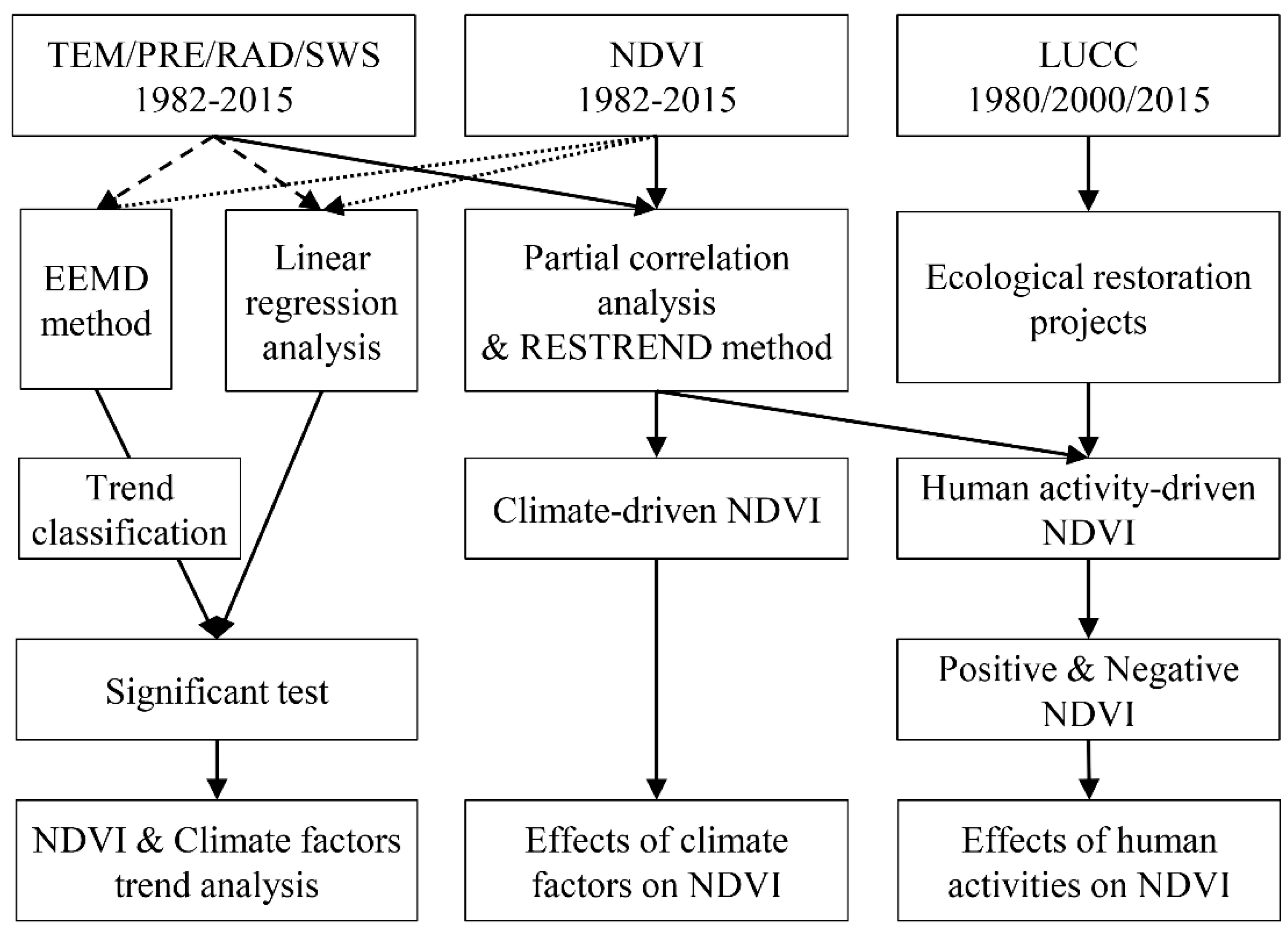
In this research, since large-scale revegetation activities were implemented in this area around 2000, the whole research period was divided into two sections to explore the impacts of anthropogenic activities on vegetation variation from 1982 to 2000 and from 2000 to 2015 (on a pixel scale). Therefore, during 1982–2000, the t₀ and t_n referred to 1982 and 2000, while during 2000–2015, the t₀ and t_n referred to 2000 and 2015, respectively. Then, the contribution rates of anthropogenic activities and land use were further superimposed to calculate the contributions of different land use changes to the NDVI. The whole workflow is shown in Figure 6.

3. Results

3.1. Temporal and Spatial Trends in the NDVI in the APENC

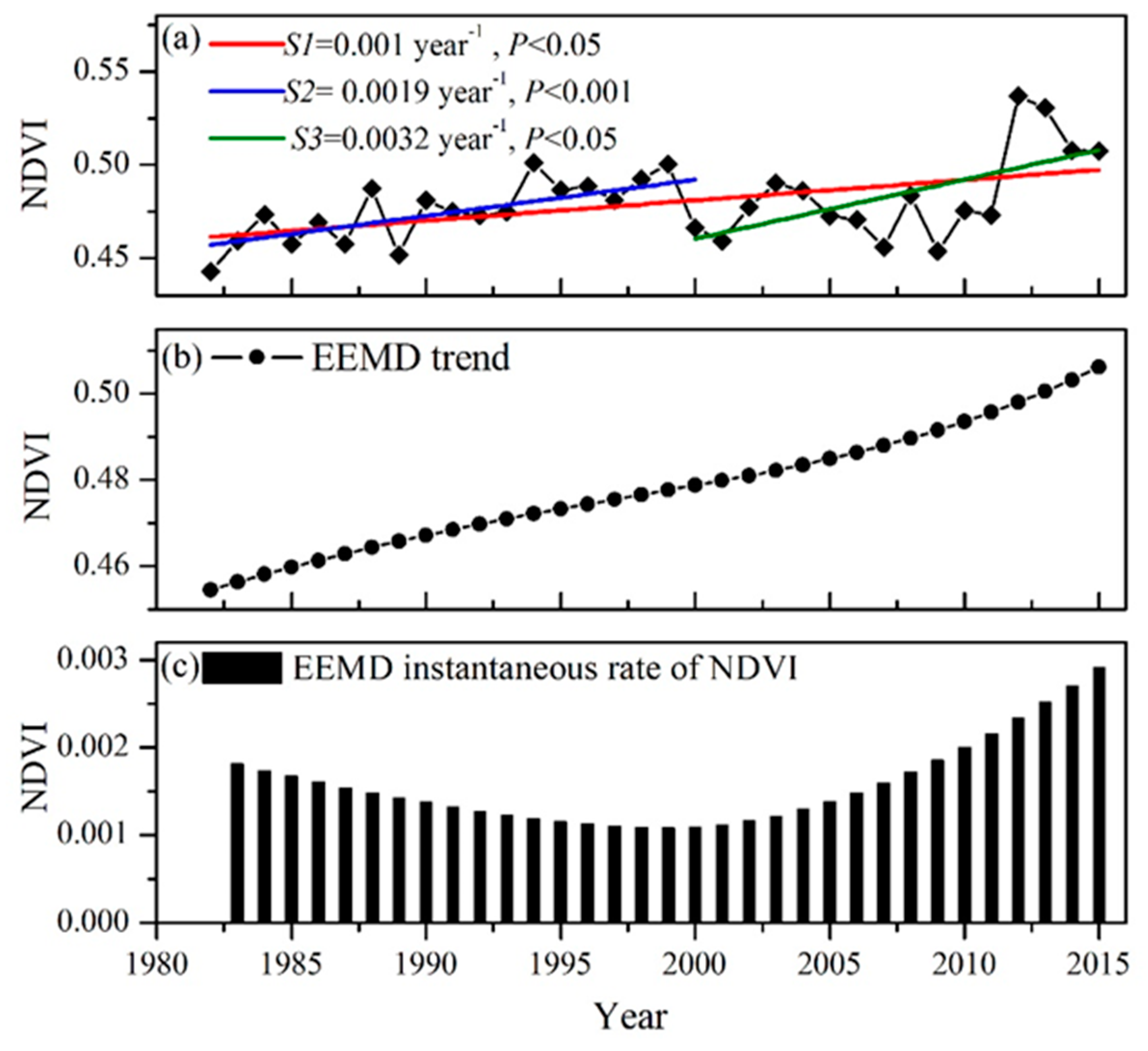
The linear and EEMD variation trends in the NDVI in the APENC are presented in Figure 7. The linear trend suggested that the annual mean NDVI of the APENC increased at a rate of 0.001 year⁻¹ (P < 0.01) during the 1982–2015 period. Compared to the NDVI before the 2000s (1982–2000), the NDVI trend rate increased by 0.0013 year⁻¹ during the 2000s (Figure 7a). Similarly, the EEMD trend presented a significant increasing trend (slope = 0.002 year⁻¹, P < 0.05) over the entire study period (Figure 7b). Nonetheless, the instantaneous greening rate first decreased and then increased, with a corresponding rate of decline from 0.002 year⁻¹ to 0.001 year⁻¹ during 1982–2000 than increased to 0.003 year⁻¹ in 2015 (Figure 7c). In general, the NDVI in the APENC continuously increased from 1982 to 2015, and the greening rate increased significantly after 2000.

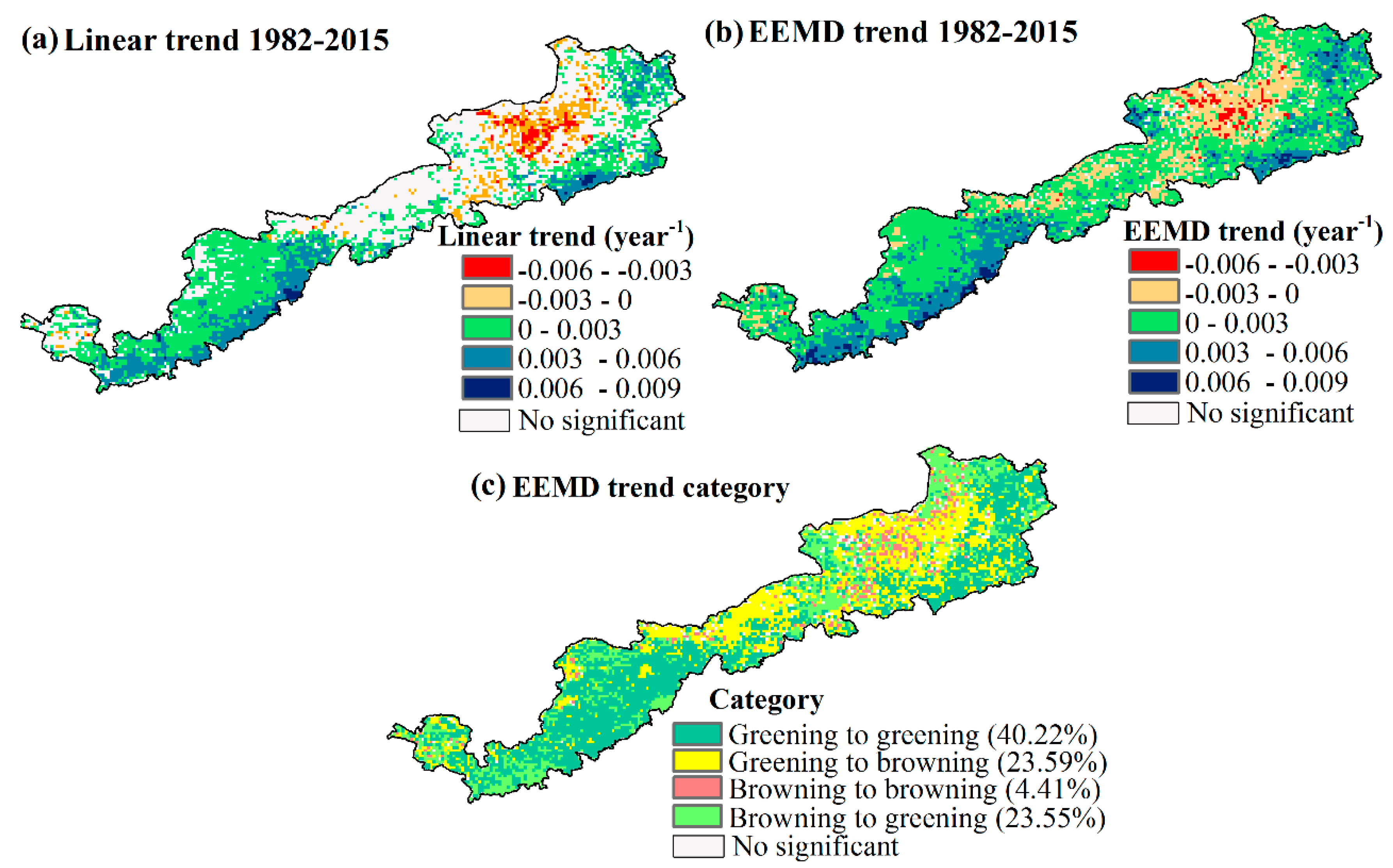
Figure 8a presents the spatial patterns of the NDVI variation trend in the APENC from 1982 to 2015. The linear trend showed that approximately 49.03% of the areas displayed a significant increase in the NDVI (slope = 0.003 year⁻¹, P < 0.05), and these areas were primarily located in the southwest and (partially) northeast of the study region, especially in the Shaanxi, Ningxia, and Gansu provinces. However, nearly 9.48% of the region had a significant vegetation browning tendency (slope = −0.002 year⁻¹, P < 0.05), which was mainly concentrated in the northeastern APENC. The remaining areas (accounting for 41.49% of the total region), distributed throughout the northcentral part of the APENC, showed no remarkable changes. Over the entire time series, approximately 96.24% of the regional NDVI that showed significant trends was detected through EEMD (Figure 8b), including 74.60% of the area experiencing greening (slope = 0.003 year⁻¹, P < 0.05) and 21.64% of the area experiencing browning (slope = 0.001 year⁻¹, P < 0.05). The spatial distribution of the EEMD trend was generally unanimous with a linear trend, except for the northcentral part of the research region, where the magnitude of the vegetation change rate was relatively low (approximately ±0.002).

In addition, the spatial trend classification of EEMD is shown in Figure 8c. Considering the spatial pattern of the EEMD trends, greening to greening was the main type, accounting for 40.97% of the vegetated area. In comparison, areas that kept browning were smaller, occupying only approximately 4.49% of the vegetated area, with a mean annual browning rate of 0.0024 year⁻¹ (P < 0.05). In addition to monotonic greening or browning, more than 49.96% of the vegetated area showed a reversed vegetation growth tendency. Roughly 26.78% and 23.99% of the vegetated area were greening to browning and browning to greening, respectively. Spatially, the greening to browning was concentrated in the northcentral part, and the browning to greening was scattered throughout the study region.

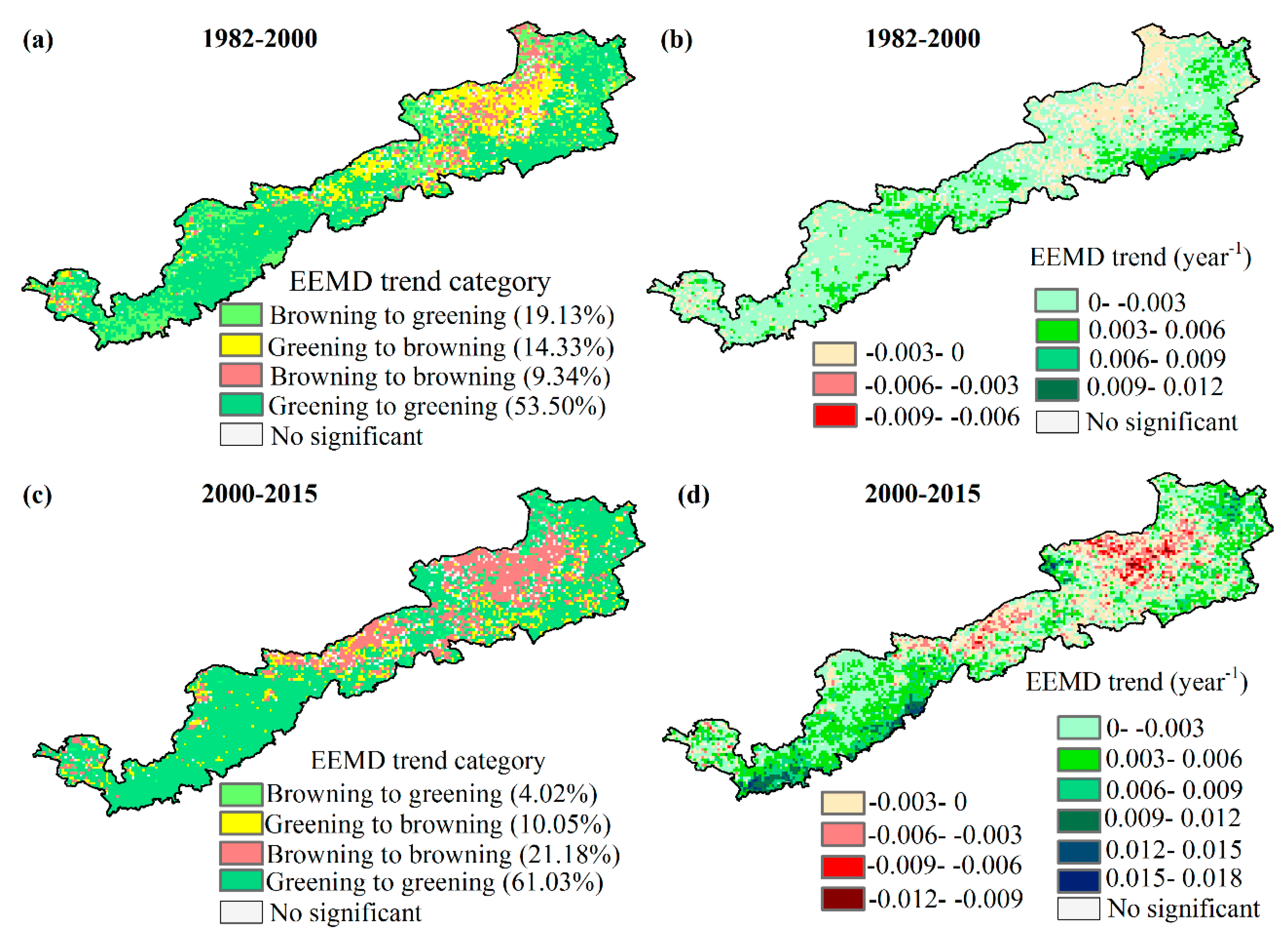
Figure 9 displays a comparison between the EEMD trend distribution and the NDVI variation rate before and after 2000. The results showed that the NDVI variation rate after 2000 (slope = 0.002 year⁻¹, P < 0.05) was significantly higher than before 2000 (slope = 0.001 year⁻¹, P < 0.05), and the areas experiencing greening to greening enlarged remarkably. However, a more noteworthy phenomenon was that browning to browning was constantly expanding around the northcentral part of the APENC, suggesting an increasing degradation rate. Overall, there were significant differences between the western and eastern parts of the study area in terms of vegetation change. That is, the grassland variability in the western part was greater than that in the eastern APENC.

3.2. Relationships between Vegetation Dynamics and Climate Change

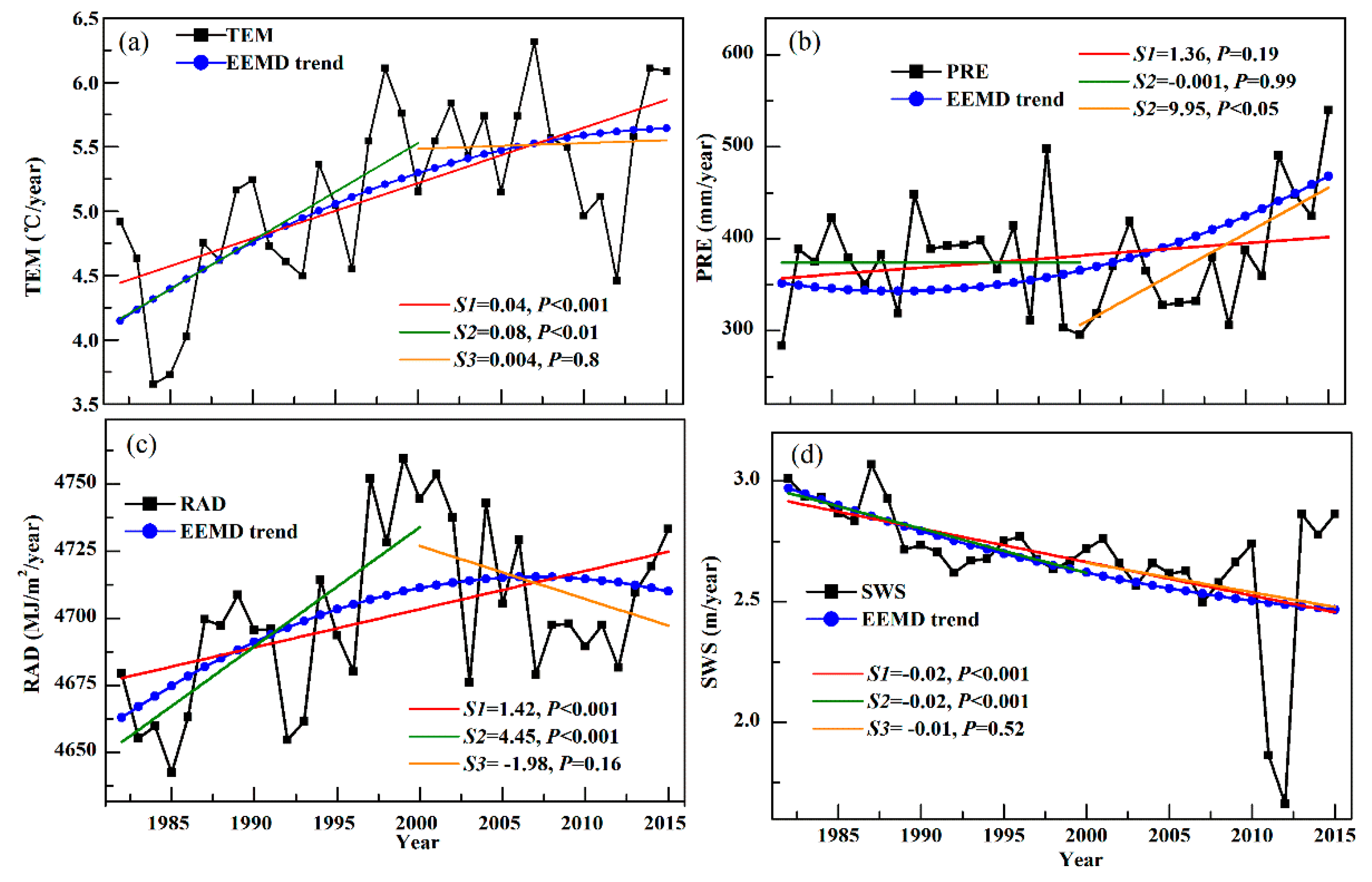
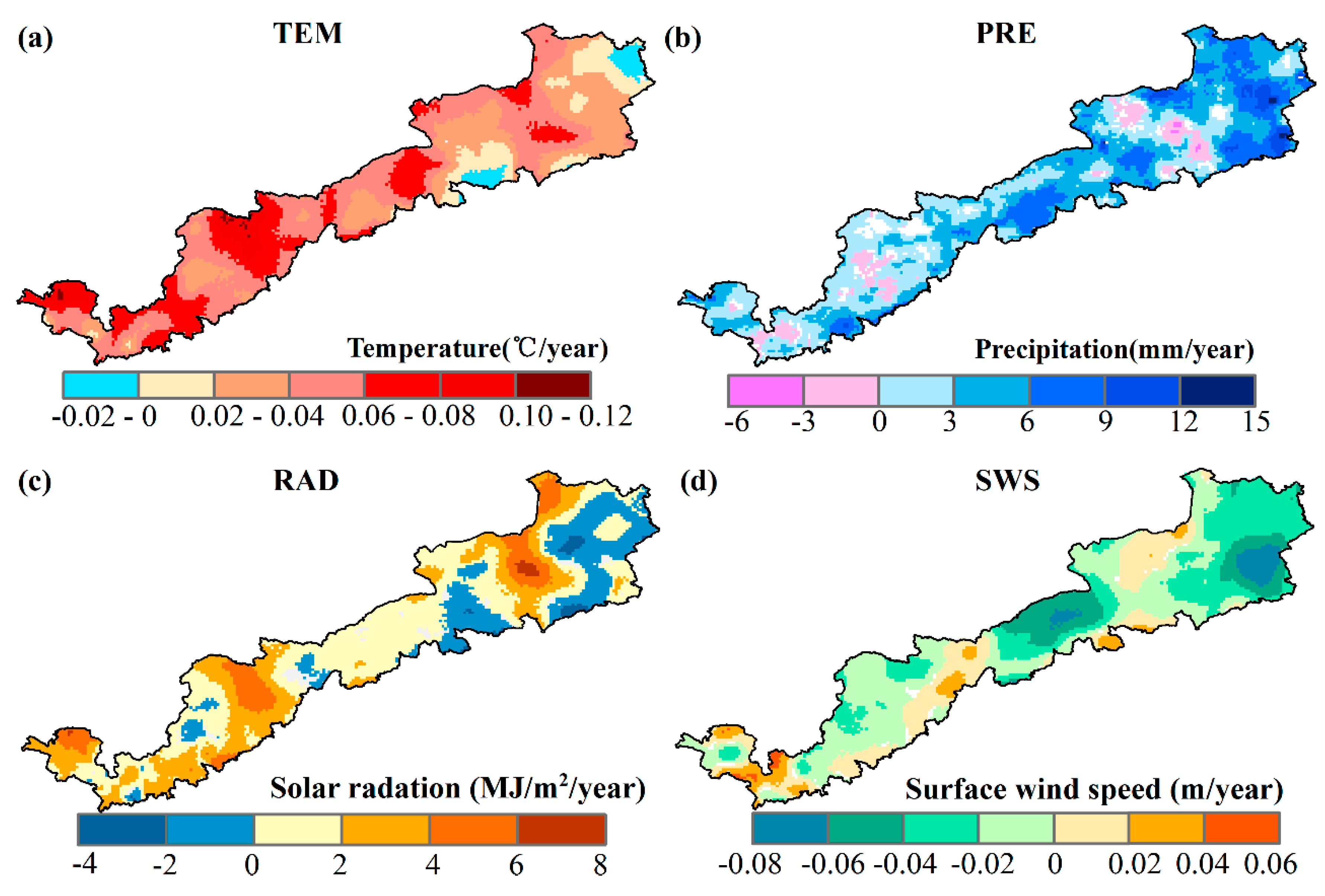
The temporal and spatial linear and EEMD trends in climatic factors are shown in Figure 10 and Figure 11. TEM, PRE, and RAD increased by 0.05 °C/year (P < 0.05), 3.54 mm/year (P < 0.05), and 1.43 MJ/m²/year (P < 0.05), respectively, during 1982–2015. Both TEM and RAD increased rapidly during 1982–2000, while after 2000, TEM was maintained at a high level and RAD declined slightly. PRE generated larger interannual fluctuations, with mean annual precipitation changes between 283.67 and 539.60 mm. The EEMD trend showed that PRE fluctuated during the entire study period, with variations that first decreased and then increased between 1982 and 2000, and a continuously increasing pattern was observed after 2000. Compared to the general upward trend in the other three meteorological factors, SWS maintained a monotonic decline during 1982–2015. Spatially, the variation trend in these climatic factors revealed an obvious spatial heterogeneity. TEM, RAD, and PRE varied with a mostly obvious zonal distribution in space. A higher warming trend occurred in the southwest, and apparent decreasing precipitation was discovered in the northcentral part of the study region. Over the whole period, SWS decreased by −0.02 m/year (P < 0.05), and a dramatic decrease was detected in the northcentral and northeastern parts of the APENC.

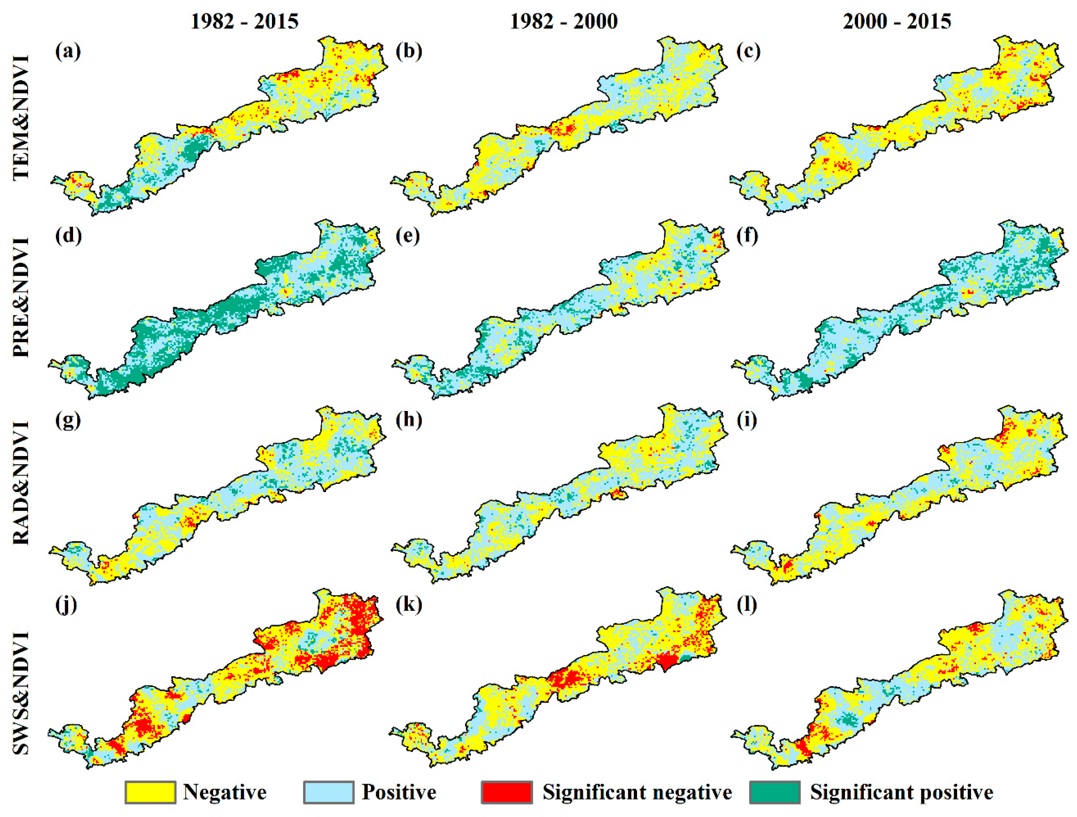
We investigated the effects of climate factors (TEM, PRE, RAD, and SWS) on NDVI variations over the entire period, and the spatial distributions of the partial correlation between the vegetation and climatic factors are shown in Figure 12. Throughout the study period, over 47.79% of the area showed that PRE had a positive effect (P < 0.05) on vegetation greening, and the mean partial correlation coefficient was more than 0.46. These areas were largely located in nonforest and nondesert areas. The positive correlation for these areas suggested that PRE was a major influential factor limiting vegetation growth. In addition, the SWS was the second most important climatic factor affecting vegetation: approximately 23.43% of the study area showed a negative correlation, mainly distributed in the northeast part of the study region. The impacts of TEM on vegetation displayed distinct north–south differences, with significant positive correlations occurring in the southwestern part (9.14%), which is dominated by cultivated farmland. A negative correlation was mainly concentrated in the northeastern part (4.01%), where grassland is the main land use type. Compared to PRE, SWS, and TEM, the effect of RAD on NDVI was quite small, with only 5.63% and 2.05% of the total area showing positive and negative correlations, respectively.

To further reveal the effect of climate on vegetation variations, we compared the partial correlation before and after 2000. For PRE, the positive effect of precipitation after 2000 was more evident than before 2000, and it increased significantly in the northeastern part of the study area. With a continuous increase in TEM, negative temperature effects on vegetation gradually appeared, especially in the central and northern parts of the APENC. The negative correlation range of temperature constantly expanded, although the correlation was not significant. We compared the effects of the SWS on vegetation before and after 2000: as the SWS decreased, the positive effects of the SWS on vegetation increased.

3.3. Relationships between Vegetation Dynamics and Anthropogenic Activity

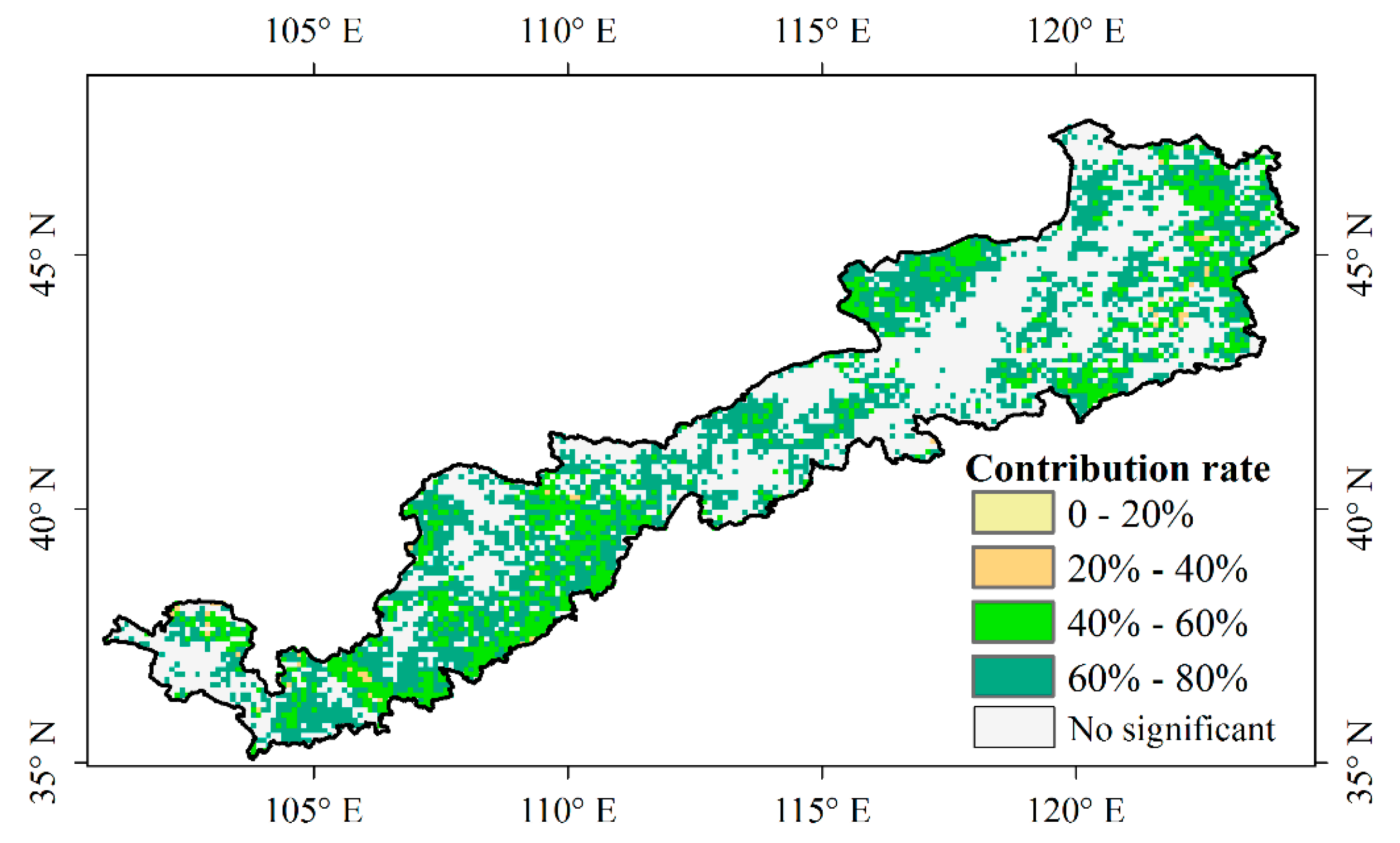
In addition to climate, anthropogenic activity is also highly important in terms of affecting vegetation variation. Based on the results of a multivariate regression analysis, the effects of climatic and anthropogenic factors on vegetation during 1982–2015 were distinguished over the entire study region. The numerical results indicated that approximately 53.85% of the APENC passed the significance test (P < 0.05), where the areas that experienced the strongest influences from climate and anthropogenic activities were distributed in the southwestern and northeastern parts of the APENC, respectively. In general, human activity contributed approximately 63.85% to vegetation variation (Figure 13).

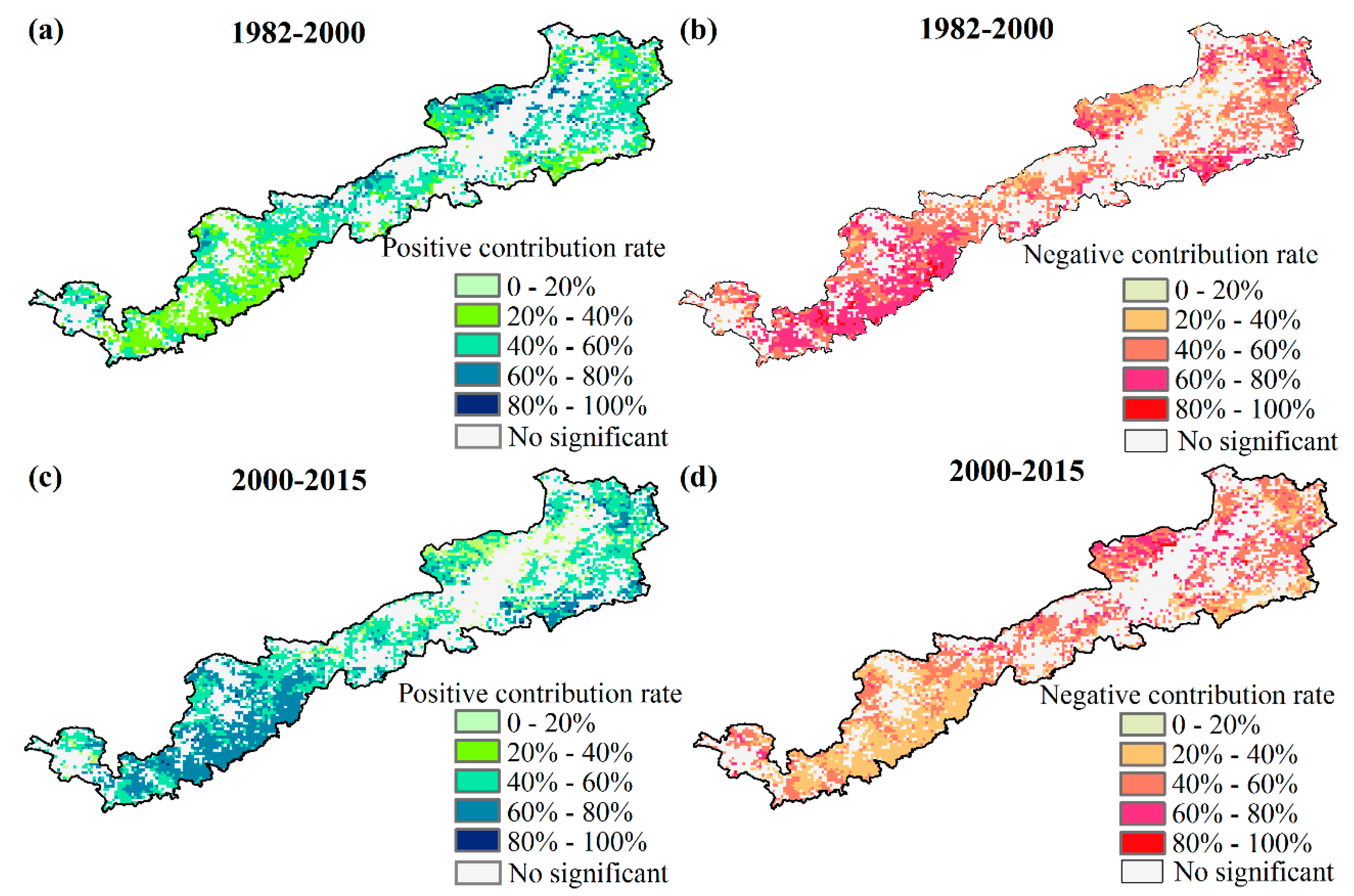
We also compared the human activity contribution rate before and after 2000 (Figure 14). The positive human activity contribution rate increased significantly after 2000, with the average contribution rate increasing from 44.16% to 54.53%, especially in the Loess Plateau located in the southwest of the APENC. On the contrary, the negative human activity contribution rate decreased from 54.54% to 45.46%. Compared to the southwestern part of the study area, the positive human activity contribution rate in the northeastern APENC was much lower, while the negative contribution of human activities increased in some areas.

Considering the impact of anthropogenic activities on vegetation, we calculated the anthropogenic contributions through land use changes during 1982–2000 and 2000–2015. The results are shown in

Table 1. Relative contribution rates of anthropogenic activities to the normalized difference vegetation index (NDVI) in the agropastoral ecotone in northern China (APENC) during the two periods.

LUCC Types	1982–2000			2000–2015
	Area (km2)	Contribution Rate		Area (km2)	Contribution Rate
		Positive	Negative		Positive	Negative
Persistent cropland	82,628	43.15%	56.85%	88,673	56.45%	43.55%
Persistent forest	20,585	49.08%	50.92%	21,624	50.01%	49.99%
Persistent water bodies	5021	43.79%	56.21%	4836	56.76%	43.24%
Persistent desert	5279	47.43%	52.57%	5578	53.36%	46.64%
Persistent construction land	36,522	44.76%	55.24%	37,154	55.15%	44.85%
Persistent high-coverage grassland	56,784	51.49%	48.51%	55,770	46.25%	53.75%
Persistent medium-coverage grassland	62,472	43.08%	56.92%	63,368	56.55%	43.45%
Persistent low-coverage grassland	40,958	40.37%	59.63%	41,652	58.65%	41.35%
Cropland → Forest	-	-	-	635	60.36%	39.64%
Cropland → Construction land	-	-	-	621	56.94%	43.06%
Cropland → High-coverage grassland	-	-	-	509	57.17%	42.83%
Cropland → Medium-coverage grassland	-	-	-	577	58.04%	41.96%
Forest → Cropland	633	46.57%	53.43%	-	-	-
Forest → Medium-coverage grassland	1611	42.94%	57.06%	-	-	-
Desert → Cropland	1112	45.80%	54.20%	604	57.39%	42.61%
Desert → Medium-coverage grassland	662	47.02%	52.98%	561	54.46%	45.54%
Desert → Low-coverage grassland	1362	35.98%	64.02%	590	52.19%	47.81%
High-coverage grassland → Cropland	3715	47.55%	52.45%	650	49.23%	50.77%
High-coverage grassland → Desert	737	45.47%	54.53%	-	-	-
High-coverage grassland → Medium coverage grassland	973	45.44%	54.56%	785	51.91%	48.09%
Medium-coverage grassland → Cropland	2291	46.10%	53.90%	527	54.85%	45.15%
Medium-coverage grassland → High-coverage grassland	-	-	-	720	54.94%	45.06%
Medium-coverage grassland → Desert	948	46.89%	53.11%	-	-	-
Medium-coverage grassland → Low-coverage grassland	930	42.70%	57.30%	524	53.31%	46.69%
Low-coverage grassland → Cropland	948	41.73%	58.27%	-	-	-
Low-coverage grassland → Desert	798	43.66%	56.34%	530	60.83%	39.17%
Low-coverage grassland → Medium-coverage grassland	-	-	-	531	56.09%	43.91%

. During 1982–2000, the negative effects of anthropogenic activities occupied a significant proportion. In the areas without land use change, persistent cropland and persistent low- and medium-coverage grassland were negatively affected by human activities, and the negative contributions were near 60% of the total anthropogenic activities. In the region that underwent land use changes, the major land use change was the conversion of grasslands (including high-, medium-, and low-coverage) to croplands, which covered an area of approximately 7.0 × 10³ km². The land use change from low-coverage grasslands to croplands was seriously influenced by human activities. However, after 2000, the negative effects from anthropogenic activities decreased, and the positive effects increased, accounting for 54.22% and 45.78% of the total anthropogenic disturbance, respectively. In the areas with no land use change, croplands, water bodies, construction lands, and medium- and low-coverage grasslands were positively affected by human activities, and the positive contribution of anthropogenic activities was more than 55% of the total anthropogenic activities. In contrast, in the areas with land use changes, the conversions between grasslands and croplands were still the main land use change type: Approximately 1.1 × 10³ km² of the croplands area was transformed to grasslands, and 1.2 × 10³ km² of the grassland area was converted to croplands, which accounted for nearly 16% of the total area during 1980–2000. Of these changes, the contributions of positive human activities caused by land use conversion from croplands to grasslands and medium-coverage grasslands to croplands were more than 57% and 54%, respectively.

4. Discussion

4.1. Advantages of the EEMD Method in Decomposition of the Vegetation Variation Trend

EEMD is among the advanced time-frequency analysis methods suitable for nonlinear and nonstationary signals in many fields, and EEMD has been introduced into vegetation dynamic research [20]. In this study, we used both linear regression and nonlinear EEMD methods to reveal the NDVI variations in the APENC from 1982 to 2015. Both methods showed that the NDVI generally increased during this period, which was consistent with the results of Liu [8]. Comparing the two methods, linear regression can directly describe the overall trend in vegetation dynamics. However, regarding nonlinear relationships between variables, linear regressions are unable to flexibly capture complex change patterns, such as those in some nonmonotonic variation areas. In contrast, the EEMD method can extract the intrinsic time trend from the long-time signal sequence and remove noise and disturbances on an interannual scale [9]. Thus, the EEMD method reflected the browning trend hidden under the greening trend in NDVI, showing that the interannual greening rate of vegetation slowed and that the area of greening to browning increased continuously from 1982 to 2000, while from 2000 to 2015, the greening trend increased and the browning trend gradually decreased. In addition, the EEMD method could break down an NDVI series into its characteristic times and apply a turning point to the temporal trend classification of the NDVI. Even in the northeastern part of the APENC, where the vegetation variation rate was small (roughly from −0.02 to 0.02 year⁻¹) (Figure 8), the EEMD method could still capture the vegetation change trend. The classification of this variation trend is helpful for understanding vegetation dynamics more intuitively.

4.2. The NDVI Response to Climate Change

Since the APENC is located on the edge of the Asian monsoon and is subjected to both the Asian Monsoon and the Western Current [50], this area is highly sensitive to climatic oscillations [51]. During the last 34 years, dramatic climate changes have occurred over the entire APENC, showing a remarkable upward tendency in the TEM, PRE, and RAD and a downward tendency in the SWS (Figure 11). The climate in northern China has changed from warm-dry to warm-wet since the late 1980s [52]. These climatic changes have observably altered plant growth [53], and the PRE influence on vegetation variation was greater than that of TEM, RAD, and SWS. Previous studies have reported that precipitation is the main limiting climatic factor affecting vegetation growth in arid and semiarid regions [54,55]. An increased PRE tendency likely results in sufficient soil moisture supplementation, but the trends in TEM and solar radiation can induce much more plant transpiration and soil evaporation [8]. Therefore, in the areas dominated by grasslands in the northeast of the APENC, for example, the TEM increase exhibited a negative effect on vegetation, especially during 1982–2000 when the TEM and RAD increased significantly, but the PRE presented a decreasing trend. As a result, a large amount of vegetation in the northeastern APENC was degraded, with most of the vegetation experiencing greening to browning during 1982–2000, with continued browning after 2000 (Figure 12). This degradation phenomenon did not weaken until the precipitation gradually increased after 2005, and this reversal phenomenon was also found in the Mongolian Plateau [56]. In contrast, in the southwestern APENC, which is dominated by arable land, the warming trend extended the grain-filling duration and thereby increased crop production [57]. On the other hand, the irrigation of arable land could also have reduced the vapor pressure deficit. In addition to precipitation, SWS was the second crucial climatic factor influencing vegetation variation, since the wind speed was negatively correlated with soil moisture content, soil texture, and nutrient content [58,59,60]. A similar result indicated that the SWS has shown a downward trend in recent decades [61]. Therefore, the decreased SWS in recent decades had a positive effect on vegetation growth from a soil moisture perspective.

4.3. NDVI Response to Anthropogenic Activities

Vegetation variation is also significantly impacted by anthropogenic activities. Accurate quantification of the impacts of anthropogenic disturbances on vegetation is beneficial to comprehensively understand vegetation variations. The residual trend method (RESTREND) has been widely used to separate anthropogenic activities from climatic effects on vegetation by developing an NDVI climatic model. Li et al. [34] and Liu et al. [49] constructed models to assess the relative contribution rates of unchanged and changed land uses to vegetation variation. Based on previous research, we improved the method to identify the effects of land use change on vegetation to further distinguish between the positive and negative effects of climatic and anthropogenic disturbances. The results suggested that anthropogenic contributions dominated the vegetation variations, which was consistent with the results of Liu et al. [8]. Before 2000, a large amount of grassland was converted to cropland, and the high-coverage grassland was degraded to low-coverage grassland, which indicated that human activities played a negative role in vegetation change. Since the economic reforms in China in 1978, croplands and livestock owned by the collectives or human communes have been redistributed to individual households [62,63]. According to economic statistics, the number of livestock increased significantly during 1982–2000 [64], which contemporaneously contributed to an obvious decrease in the NDVI magnitude. Therefore, extensive cultivation and overgrazing were important causes of vegetation degradation during 1982–2000.

After 2000, a series of land use changes were implemented in the degraded grasslands, including land use conversions from croplands and desert to grasslands and from low-coverage grassland to high-coverage grassland. The positive human contribution rate significantly increased, especially in the Loess Plateau located in the southwestern APENC. These land use changes were attributed to the implementation of ecological restoration strategies (i.e., the Grain to Green Program and the Returning Grazing Land to Grassland Policy), and land rehabilitation has been obviously increasing since the 2000s [65]. In 2003, “grassland transfer” policies were proposed in agricultural and pastoral areas in many provinces, including Inner Mongolia, Shaanxi, Ningxia, Gansu, and Xinjiang [42]. Based on these policies, grasslands gradually underwent rehabilitation: Both high-coverage and medium-coverage grasslands tended to increase [66], and croplands and desert were returned to grasslands and wetlands gradually [67]. Therefore, the negative human contribution rate decreased in the northeast of the APENC. However, a significant cropland expansion was also detected in the northeastern part of the study area and was mainly converted from grasslands. Wei et al. [68] indicated that the abolition of an agricultural tax and the implementation of a farmland protection system by the Chinese government were crucial reasons for cropland areas rebounding.

4.4. Limitations of the Study

In this study, we first used the RESTREND method to separate the vegetation changes induced by climatic or anthropogenic factors and further distinguished the positive and negative contributions of anthropogenic activities. The results revealed some differences in the effects of climatic factors and anthropogenic activities on vegetation change. Although the RESTREND method has been extensively applied to study vegetation change, the method still contains some drawbacks. On the one hand, in the establishment of the regression equation of climatic factors and the NDVI, the proportions of pixels with statistical significance showed an important relationship with the time period of the regression equation [69]. To solve this problem, in our study, we attempted to use a longer time scale to reduce the method’s biases. On the other hand, the selection of climatic factors had an important influence on the inverse mode of the climate-driven NDVI. In this paper, we chose four major climatic factors (PRE, TEM, RAD and SWS), and of course, other climatic factors may also have had an impact on the vegetation change in this region. Therefore, in future studies, more climatic factors need to be applied to analyze climate effects on NDVI variations, which may increase the proportion of the NDVI explained by climatic factors via linear regression. Considering additional climatic factors can also help to comprehensively understand the relationship between vegetation and climate and more accurately assess the contribution of human activity to vegetation change.

5. Conclusions

In this study, we used the EEMD method to assess the spatiotemporal dynamics of vegetation variation in the agropastoral ecotone of northern China during 1982–2015. Subsequently, we also distinguished and quantified the relative effects of climatic and anthropogenic factors on vegetation variation. The results showed that most areas of the APENC experienced a monotonous greening trend throughout the entire study period. However, under the background of the overall greening trend, there was a notable trend of vegetation browning in the northern and central parts of the study area. The NDVI and precipitation presented a remarkable spatiotemporal correlation, suggesting that precipitation was the main climatic driver over the whole area. Additionally, a decrease in precipitation and an increase in temperature were two important reasons for vegetation degradation in the northcentral part of the APENC. Subsequently, the RESTREND results indicated that anthropogenic activity was the major driving factor (63.85%) of vegetation variation, and the positive human contribution rate significantly increased after 2000, especially in the southwest of the APENC.

References

1. Dong, J.; Tao, F.; Zhang, G. Trends and variation in vegetation greenness related to geographic controls in middle and eastern Inner Mongolia, China. Environ. Earth Sci. 2011, 62, 245–256. [Google Scholar] [CrossRef]
2. Li, X.L.; Yang, L.X.; Tian, W.; Xu, X.F.; He, C.S. Land use and land cover change in agro-pastoral ecotone in Northern China: A review. Chin. J. Appl. Ecol. 2018, 29, 3487–3495. [Google Scholar]
3. Li, Q.; Zhang, X.F.; Liu, Q.F.; Liu, Y.; Ding, Y.; Zhang, Q. Impact of Land Use Intensity on Ecosystem Services: An Example from the Agro-Pastoral Ecotone of Central Inner Mongolia. Sustainability 2017, 9, 1030. [Google Scholar] [CrossRef]
4. Yang, Y.J.; Wang, K.; Liu, D.; Zhao, X.Q.; Fang, J.W.; Li, J.S.; Zhai, X.J.; Zhang, C.; Zhan, R.Y. Spatiotemporal Variation Characteristics of Ecosystem Service Losses in the Agro-Pastoral Ecotone of Northern China. Int. J. Environ. Res. Public Health 2019, 16, 1199. [Google Scholar] [CrossRef] [PubMed]
5. Peng, J.; Li, Y.; Tian, L.; Liu, Y.X.; Wang, Y.L. Vegetation Dynamics and Associated Driving Forces in Eastern China during 1999–2008. Remote Sens. 2015, 7, 13641–13663. [Google Scholar] [CrossRef]
6. Liu, H.Y.; Zhang, M.Y.; Lin, Z.S.; Xu, X.J. Spatial heterogeneity of the relationship between vegetation dynamics and climate change and their driving forces at multiple time scales in Southwest China. Agric. For. Meteorol. 2018, 256, 10–21. [Google Scholar] [CrossRef]
7. Fang, X.Q.; Zhu, Q.A.; Ren, L.L.; Chen, H.; Wang, K.; Peng, C.H. Large-scale detection of vegetation dynamics and their potential drivers using MODIS images and BFAST: A case study in Quebec, Canada. Remote Sens. Environ. 2018, 206, 391–402. [Google Scholar] [CrossRef]
8. Liu, Z.J.; Liu, Y.S.; Li, Y.R. Anthropogenic contributions dominate trends of vegetation cover change over the farming-pastoral ecotone of northern China. Ecol. Indic. 2018, 95, 370–378. [Google Scholar] [CrossRef]
9. Pan, N.Q.; Feng, X.M.; Fu, B.J.; Wang, S.; Ji, F.; Pan, S.F. Increasing global vegetation browning hidden in overall vegetation greening: Insights from time-varying trends. Remote Sens. Environ. 2018, 214, 59–72. [Google Scholar] [CrossRef]
10. Gonsamo, A.; Chen, J.M.; D’Odorico, P. Underestimated role of East Atlantic-West Russia pattern on Amazon vegetation productivity. Proc. Natl. Acad. Sci. USA 2015, 112, E1054–E1055. [Google Scholar] [CrossRef]
11. Ju, J.C.; Masek, J.G. The vegetation greenness trend in Canada and US Alaska from 1984–2012 Landsat data. Remote Sens. Environ. 2016, 176, 1–16. [Google Scholar] [CrossRef]
12. Neigh, C.S.R.; Tucker, C.J.; Townshend, J.R.G. North American vegetation dynamics observed with multi-resolution satellite data. Remote Sens. Environ. 2008, 112, 1749–1772. [Google Scholar] [CrossRef] [Green Version]
13. Bhavani, P.; Roy, P.S.; Chakravarthi, V.; Kanawade, V.P. Satellite Remote Sensing for Monitoring Agriculture Growth and Agricultural Drought Vulnerability Using Long-Term (1982–2015) Climate Variability and Socio-economic Data set. Proc. Natl. Acad. Sci. India Sect. 2017, 87, 733–750. [Google Scholar] [CrossRef]
14. Gonsamo, A.; D’Odorico, P.; Chen, J.M.; Wu, C.; Buchmann, N. Changes in vegetation phenology are not reflected in atmospheric CO2 and 13C/12C seasonality. Glob. Chang. Biol. 2017, 23, 4029–4044. [Google Scholar] [CrossRef] [PubMed]
15. Hellden, U.; Tottrup, C. Regional desertification: A global synthesis. Glob. Planet. Chang. 2008, 64, 169–176. [Google Scholar] [CrossRef]
16. Jamali, S.; Jonsson, P.; Eklundh, L.; Ardo, J.; Seaquist, J. Detecting changes in vegetation trends using time series segmentation. Remote Sens. Environ. 2015, 156, 182–195. [Google Scholar] [CrossRef]
17. Martinez, B.; Gilabert, M.A. Vegetation dynamics from NDVI time series analysis using the wavelet transform. Remote Sens. Environ. 2009, 113, 1823–1842. [Google Scholar] [CrossRef]
18. Roerink, G.J.; Menenti, M.; Soepboer, W.; Su, Z. Assessment of climate impact on vegetation dynamics by using remote sensing. Phys. Chem. Earth 2003, 28, 103–109. [Google Scholar] [CrossRef]
19. Torrence, C.; Compo, C.P. A practical guide to wavelet analysis. Bull. Am. Meteorol. Soc. 1998, 79, 61–78. [Google Scholar] [CrossRef]
20. Verbesselt, J.; Hyndman, R.; Newnham, G.; Culvenor, D. Detecting trend and seasonal changes in satellite image time series. Remote Sens. Environ. 2010, 114, 106–115. [Google Scholar] [CrossRef]
21. Wang, K.S.; Heyns, P.S. The combined use of order tracking techniques for enhanced Fourier analysis of order components. Mech. Syst. Sig. Process. 2011, 25, 803–811. [Google Scholar] [CrossRef] [Green Version]
22. Liu, H.M.; Zhang, Q.M.; Yang, C.; Wang, J. The multi-timescale temporal patterns and dynamics of land surface temperature using Ensemble Empirical Mode Decomposition. Sci. Total Environ. 2019, 265, 243–255. [Google Scholar] [CrossRef] [PubMed]
23. Jamali, S.; Seaquist, J.; Eklundh, L.; Ardö, J. Automated mapping of vegetation trends with polynomials using NDVI imagery over the Sahel. Remote Sens. Environ. 2014, 141, 79–89. [Google Scholar] [CrossRef]
24. Yin, Y.H.; Ma, D.D.; Wu, S.L.; Dai, E.F.; Zhu, Z.C.; Myneni, B.R. Nonlinear variations of forest leaf area index over China during 1982–2010 based on EEMD method. Int. J. Biometeorol. 2017, 61, 977–988. [Google Scholar] [CrossRef] [PubMed]
25. Wu, Z.; Huang, N. Ensemble Empirical Mode Decomposition: A Noise-Assisted Data Analysis Method. Adv. Adapt. Data Anal. 2009, 1, 1–41. [Google Scholar] [CrossRef]
26. Wang, W.C.; Chau, K.W.; Xu, D.M.; Chen, X.Y. Improving Forecasting Accuracy of Annual Runoff Time Series Using ARIMA Based on EEMD Decomposition. Water Resour. Manag. 2015, 29, 2655–2675. [Google Scholar] [CrossRef]
27. Liu, Q.J.; Zhang, H.Y.; Gao, K.T.; Xu, B.; Wu, J.Z.; Fang, N.F. Time-frequency analysis and simulation of the watershed suspended sediment concentration based on the Hilbert-Huang transform (HHT) and artificial neural network (ANN) methods: A case study in the Loess Plateau of China. Catena 2019, 179, 107–118. [Google Scholar] [CrossRef]
28. Ji, Q.; Geng, J.-B.; Tiwari, A.K. Information spillovers and connectedness networks in the oil and gas markets. Energy Econ. 2018, 75, 71–84. [Google Scholar] [CrossRef]
29. Rai, A.; Upadhyay, S.H. An integrated approach to bearing prognostics based on EEMD-multi feature extraction, Gaussian mixture models and Jensen-Renyi divergence. Appl. Soft Comput. 2018, 71, 36–50. [Google Scholar] [CrossRef]
30. Sun, W.; Wang, C.F. Staged icing forecasting of power transmission lines based on icing cycle and improved extreme learning machine. J. Clean. Prod. 2019, 208, 1384–1392. [Google Scholar] [CrossRef]
31. Xian, L.; He, K.J.; Lai, K.K. Gold price analysis based on ensemble empirical model decomposition and independent component analysis. Physica A Stat. Mech. Appl. 2016, 454, 11–23. [Google Scholar] [CrossRef]
32. Kong, Y.L.; Meng, Y.; Li, W.; Yue, A.Z.; Yuan, Y. Satellite Image Time Series Decomposition Based on EEMD. Remote Sens. 2015, 7, 15583–15604. [Google Scholar] [CrossRef] [Green Version]
33. Ren, H.; Wang, Y.L.; Huang, M.Y.; Chang, Y.L.; Kao, H.M. Ensemble Empirical Mode Decomposition Parameters Optimization for Spectral Distance Measurement in Hyperspectral Remote Sensing Data. Remote Sens. 2014, 6, 2069–2083. [Google Scholar] [CrossRef] [Green Version]
34. Li, Y.R.; Cao, Z.; Long, H.L.; Liu, Y.S.; Li, W.J. Dynamic analysis of ecological environment combined with land cover and NDVI changes and implications for sustainable urban-rural development: The case of Mu Us Sandy Land, China. J. Clean. Prod. 2017, 142, 697–715. [Google Scholar] [CrossRef]
35. Robinson, B.E.; Li, P.; Hou, X.Y. Institutional change in social-ecological systems: The evolution of grassland management in Inner Mongolia. Glob. Environ. Chang. 2017, 47, 64–75. [Google Scholar] [CrossRef]
36. Tong, S.; Zhang, J.; Bao, Y.; Lai, Q.; Lian, X.; Li, N.; Bao, Y. Analyzing vegetation dynamic trend on the Mongolian Plateau based on the Hurst exponent and influencing factors from 1982–2013. J. Geogr. Sci. 2018, 28, 595–610. [Google Scholar] [CrossRef]
37. Jiang, Z.; Huete, A.R.; Chen, J.; Chen, Y.; Li, J.; Yan, G.; Zhang, X. Analysis of NDVI and scaled difference vegetation index retrievals of vegetation fraction. Remote Sens. Environ. 2006, 101, 366–378. [Google Scholar] [CrossRef]
38. Li, S.C.; Zhao, Z.Q.; Liu, F.Y. Identifying spatial pattern of NDVI series dynamics using recurrence quantification analysis. Eur. Phys. J. Spec. Top. 2008, 164, 127–139. [Google Scholar] [CrossRef]
39. Gichenje, H.; Godinho, S. Establishing a land degradation neutrality national baseline through trend analysis of GIMMS NDVI Time-series. Land Degrad. Dev. 2018, 29, 2985–2997. [Google Scholar] [CrossRef]
40. Chen, Y.Y.; Yang, K.; He, J.; Qin, J.; Shi, J.C.; Du, J.Y.; Qing, H. Improve land surface temperature modeling for dry land of China. J. Geophys. Res. 2011, 116, D20. [Google Scholar] [CrossRef]
41. Liu, Q.; Fu, Y.H.S.; Zeng, Z.Z.; Huang, M.T.; Li, X.R.; Piao, S.L. Temperature, precipitation, and insolation on autumn vegetation phenology in temperature China. Glob. Chang. Biol. 2016, 22, 644–655. [Google Scholar] [CrossRef] [PubMed]
42. Yao, Y.; Zhao, S.; Zhang, Y.; Jia, K.; Liu, M. Spatial and Decadal Variations in Potential Evapotranspiration of China Based on Reanalysis Datasets during 1982–2010. Atmosphere 2014, 5, 737–754. [Google Scholar] [CrossRef]
43. Liu, J.; Ning, J.; Kuang, W.; Xu, X.; Zhang, S.; Yan, C.; Li, R.D.; Hu, Y.F.; Du, G.M.; Chi, W.; et al. Spatio-temporal patterns and characteristics of land–use change in China during 2010–2015. J. Geogr. Sci. 2018, 73, 789–802. [Google Scholar]
44. Huang, N.E.; Shen, Z.; Long, S.R.; Wu, M.L.C.; Shih, H.H.; Zheng, Q.N.; Yen, N.C.; Tung, C.C.; Liu, H.H. The empirical mode decomposition and the Hilbert spectrum for nonlinear and non-stationary time series analysis. Proc. R. Soc. A 1998, 454, 903–995. [Google Scholar] [CrossRef]
45. Wei, F.L.; Wang, S.; Fu, B.J.; Pan, N.Q.; Feng, X.M.; Zhao, W.W.; Wang, C. Vegetation dynamic trends and the main drivers detected using the ensemble empirical mode decomposition method in East Africa. Land Degrad. Dev. 2018, 29, 2542–2553. [Google Scholar] [CrossRef]
46. Peng, J.; Liu, Z.H.; Liu, Y.H.; Wu, J.S.; Han, Y.N. Trend analysis of vegetation dynamics in Qinghai–Tibet Plateau using Hurst Exponent. Ecol. Indic. 2012, 14, 28–39. [Google Scholar] [CrossRef]
47. Wessels, K.J.; Prince, S.D.; Malherbe, J.; Small, J.; Frost, P.E.; VanZyl, D. Can human-induced land degradation be distinguished from the effects of rainfall variability? A case study in South Africa. J. Arid. Environ. 2007, 68, 271–297. [Google Scholar] [CrossRef]
48. Wessels, K.J.; Van Den Bergh, F.; Scholes, R.J. Limits to detectability of land degradation by trend analysis of vegetation index data. Remote Sens. Environ. 2012, 125, 10–22. [Google Scholar] [CrossRef]
49. Liu, R.; Xiao, L.; Liu, Z.; Dai, J. Quantifying the relative impacts of climate and human activities on vegetation changes at the regional scale. Ecol. Indic. 2018, 93, 91–99. [Google Scholar] [CrossRef]
50. Chen, J.; Wei, H.; Jin, L.Y.; Chen, J.H.; Chen, S.Q.; Chen, F.H. A climatological northern boundary index for the East Asian summer monsoon and its interannual variability. Sci. China Earth Sci. 2018, 61, 13–22. [Google Scholar] [CrossRef]
51. Qian, W.H.; Lin, X.; Zhu, Y.F.; Xu, Y.; Fu, J.L. Climatic regime shift and decadal anomalous events in China. Clim. Chang. 2007, 84, 167–189. [Google Scholar] [CrossRef]
52. Huang, W.; Chen, F.H.; Feng, S.; Chen, J.H.; Zhang, X.J. Interannual precipitation variations in the mid-latitude Asia and their association with large-scale atmospheric circulation. Chin. Sci. Bull. 2013, 58, 3962–3968. [Google Scholar] [CrossRef] [Green Version]
53. Chen, B.Z.; Xu, G.; Coops, N.C.; Ciais, P.; Innes, J.L.; Wang, G.Y.; Myneni, R.B.; Wang, T.L.; Krzyzanowski, J.; Li, Q.L.; et al. Changes in vegetation photosynthetic activity trends across the Asia-Pacific region over the last three decades. Remote Sens. Environ. 2014, 144, 28–41. [Google Scholar] [CrossRef]
54. Duan, H.C.; Yan, C.Z.; Tsunekawa, A.; Song, X.; Li, S.; Xie, J.L. Assessing vegetation dynamics in the Three-North Shelter Forest region of China using AVHRR NDVI data. Environ. Earth Sci. 2011, 64, 1011–1020. [Google Scholar] [CrossRef]
55. Miao, L.J.; Jiang, C.; Xue, B.L.; Liu, Q.; He, B.; Nath, R.; Cui, X.F. Vegetation dynamics and factor analysis in arid and semi-arid Inner Mongolia. Environ. Earth Sci. 2015, 73, 2343–2352. [Google Scholar] [CrossRef]
56. Bao, G.; Qin, Z.; Bao, Y.; Zhou, Y.; Li, W.; Sanjjav, A. NDVI-Based Long-Term Vegetation Dynamics and Its Response to Climatic Change in the Mongolian Plateau. Remote Sens. 2014, 6, 8337–8358. [Google Scholar] [CrossRef] [Green Version]
57. Qiao, J.M.; Yu, D.Y.; Wang, Q.F.; Liu, Y.P. Diverse effects of crop distribution and climate change on crop production in the agro-pastoral transitional zone of China. Front. Earth Sci. 2018, 12, 408–419. [Google Scholar] [CrossRef]
58. Du, H.; Zuo, X.; Li, S.; Wang, T.; Xue, X. Wind erosion changes induced by different grazing intensities in the desert steppe, Northern China. Agric. Ecosyst. Environ. 2019, 274, 1–13. [Google Scholar] [CrossRef]
59. Meng, Z.J.; Dang, X.H.; Gao, Y.; Ren, X.M.; Ding, Y.L.; Wang, M. Interactive effects of wind speed, vegetation coverage and soil moisture in controlling wind erosion in a temperate desert steppe, Inner Mongolia of China. J. Arid. Land 2018, 10, 534–547. [Google Scholar] [CrossRef] [Green Version]
60. Nourzadeh, M.; Bahrami, H.A.; Goossens, D.; Fryrear, D.W. Determining soil erosion and threshold friction velocity at different soil moisture conditions using a portable wind tunnel. Z. Geomorphol. 2013, 57, 97–109. [Google Scholar] [CrossRef]
61. Zhang, G.; Azorin-Molina, C.; Shi, P.; Lin, D.; Guijarro, J.A.; Kong, F.; Chen, D. Impact of near-surface wind speed variability on wind erosion in the eastern agro-pastoral transitional zone of Northern China, 1982–2016. Agric. For. Meteorol. 2019, 271, 102–115. [Google Scholar] [CrossRef]
62. Hua, L.; Squires, V.R. Managing China’s pastoral lands: Current problems and future prospects. Land Use Pol. 2015, 43, 129–137. [Google Scholar] [CrossRef]
63. Zhang, L.X.; Yang, Z.F.; Chen, G.Q. Emergy analysis of cropping–grazing system in Inner Mongolia Autonomous Region, China. Energy Policy 2007, 35, 3843–3855. [Google Scholar] [CrossRef]
64. Jiang, H. Decentralization, Ecological Construction, and the Environment in Post-Reform China: Case Study from Uxin Banner, Inner Mongolia. World Dev. 2006, 34, 1907–1921. [Google Scholar] [CrossRef]
65. Yeh, E.T. Greening western China: A critical view. Geoforum 2009, 40, 884–894. [Google Scholar] [CrossRef]
66. Nendel, C.; Hu, Y.; Lakes, T. Land-use change and land degradation on the Mongolian Plateau from 1975 to 2015-A case study from Xilingol, China. Land Degrad. Dev. 2018, 29, 1595–1606. [Google Scholar]
67. Mao, D.H.; Wang, Z.M.; Wu, B.F.; Zeng, Y.; Luo, L.; Zhang, B. Land degradation and restoration in the arid and semiarid zones of China: Quantified evidence and implications from satellites. Land Degrad. Dev. 2018, 29, 3841–3851. [Google Scholar] [CrossRef]
68. Wei, B.; Xie, Y.; Jia, X.; Wang, X.; He, H.; Xue, X. Land use/land cover change and it’s impacts on diurnal temperature range over the agricultural pastoral ecotone of Northern China. Land Degrad. Dev. 2018, 29, 3009–3020. [Google Scholar] [CrossRef]
69. Li, A.; Wu, J.G.; Huang, J.H. Distinguishing between human-induced and climate-driven vegetation changes: A critical application of RESTREND in Inner Mongolia. Landsc. Ecol. 2012, 27, 969–982. [Google Scholar] [CrossRef]
Figure 1. Location of the agropastoral ecotone in northern China (APENC) and land use and land cover types in 2015.
Remotesensing 11 01860 g001
Figure 2. Distribution of the Global Inventory Modeling and Mapping Studies (GIMMS NDVI3g) product (a) and China Meteorological Forcing Dataset (CMFD) climate data samples (temperature (TEM), precipitation (PRE), total downward solar radiation (RAD), and near-surface wind speed (SWS)) (be). The magnified figures below each index represent the three corresponding random regions, named A, B, and C from the west to the east.
Remotesensing 11 01860 g002
Figure 3. Land use and land cover (LUCC) types conversion between (a) 1982 and 2000 and (b) 2000 and 2015. CCR is croplands, FRO is forests, URB is urban construction lands, DES is deserts, HCG is high-coverage grasslands, MCG is medium-coverage grasslands, and LCG is low-coverage grasslands.
Remotesensing 11 01860 g003
Figure 4. A flow chart of the ensemble empirical mode decomposition (EEMD) method.
Remotesensing 11 01860 g004
Figure 5. Temporal normalized difference vegetation index (NDVI) classified by the EEMD technique.
Remotesensing 11 01860 g005
Figure 6. Workflow of the NDVI analysis methods and processes.
Remotesensing 11 01860 g006
Figure 7. Annual NDVI trend during 1982–2015: (a) the S1, S2, and S3 mean linear trends of the mean NDVI during 1982–2015, 1982–2000, and 2000–2015, respectively; (b) the EEMD trend; and (c) the interannual instantaneous rate of EEMD.
Remotesensing 11 01860 g007
Figure 8. Spatial distribution of linear trends (a) and EEMD trends (b) in the NDVI during 1982–2015, and the EEMD trend classification in the APENC (c). Only pixels with P < 0.05 are presented.
Remotesensing 11 01860 g008
Figure 9. Spatial distribution of the EEMD trend classification (a,c) and variation rate (b,d) before and after 2000. Only pixels with P < 0.05 are presented.
Remotesensing 11 01860 g009
Figure 10. The temporal trend of temperature (TEM) (a), precipitation (PRE) (b), total downward solar radiation (RAD) (c), and near-surface wind speed (SWS) (d) in the APENC from 1982 to 2015. S1, S2, and S3 represent the slope of each variable from 1982 to 2015, 1982 to 2000, and 2000 to 2015, respectively. Only pixels with P < 0.05 are represented.
Remotesensing 11 01860 g010
Figure 11. The spatiotemporal distribution of TEM (a), PRE (b), RAD (c), and SWS (d) in the APENC from 1982 to 2015. The insets show the temporal variations of each variable, and S1, S2, and S3 represent the slope in 1982–2015, 1982–2000, and 2000–2015, respectively. Only pixels with a P < 0.05 are represented.
Remotesensing 11 01860 g011
Figure 12. Spatial distribution of partial correlations between the NDVI and relevant climatic factors (TEM (ac), PRE (df), RAD (gi), and SWS (jl)) in the APENC from 1982 to 2015 (significance level at P < 0.05).
Remotesensing 11 01860 g012
Figure 13. Spatial distribution of the total human activity contribution rate to NDVI dynamics during 1982–2015. Only pixels with P < 0.05 were presented.
Remotesensing 11 01860 g013
Figure 14. Spatial distribution of the positive (a,c) and negative (b,d) contribution rate to NDVI dynamics of human activities before and after 2000. Only pixels with P < 0.05 are presented.
Remotesensing 11 01860 g014