Letter

Application of Laplace Domain Waveform Inversion to Cross-Hole Radar Data

1
State Key Laboratory of Lunar and Planetary Sciences, Macau University of Science and Technology, Macau, China
2
College of Geo-Exploration Science and Technology, Jilin University, Changchun 130026, China
3
Department of Earth and Space Sciences, Southern University of Science and Technology, Shenzhen 518055, China
*
Author to whom correspondence should be addressed.
Remote Sens. 2019, 11(16), 1839; https://doi.org/10.3390/rs11161839
Submission received: 11 June 2019 / Revised: 8 July 2019 / Accepted: 31 July 2019 / Published: 7 August 2019
(This article belongs to the Special Issue Recent Progress in Ground Penetrating Radar Remote Sensing)

Abstract

:
Full waveform inversion (FWI) can yield high resolution images and has been applied in Ground Penetrating Radar (GPR) for around 20 years. However, appropriate selection of the initial models is important in FWI because such an inversion is highly nonlinear. The conventional way to obtain the initial models for GPR FWI is ray-based tomogram inversion which suffers from several inherent shortcomings. In this paper, we develop a Laplace domain waveform inversion to obtain initial models for the time domain FWI. The gradient expression of the Laplace domain waveform inversion is deduced via the derivation of a logarithmic object function. Permittivity and conductivity are updated by using the conjugate gradient method. Using synthetic examples, we found that the value of the damping constant in the inversion cannot be too large or too small compared to the dominant frequency of the radar data. The synthetic examples demonstrate that the Laplace domain waveform inversion provide slightly better initial models for the time domain FWI than the ray-based inversion. Finally, we successfully applied the algorithm to one field data set, and the inverted results of the Laplace-based FWI show more details than that of the ray-based FWI.

Graphical Abstract

1. Introduction

Ground Penetrating Radar (GPR) is extensively applied in archaeological, environmental, hydrological and engineering investigations to detect subsurface structures [1]. Cross-hole radar (normally 20–250 MHz), with transmitting antennas in a borehole and receiving antennas in a second, neighboring borehole, can provide high-resolution tomographic images of permittivity ( ε ) and conductivity ( σ ) between the two boreholes.
Traditional radar tomographic inversions, such as travel time inversion and attenuation inversion, are based on geometrical ray theory [2,3,4,5,6,7]. The resolution of ray theory tomography is around the width of the first Fresnel-zone [8,9]. Full-waveform inversion (FWI) was first applied in seismic exploration (e.g., [10,11,12]) and was subsequently introduced to GPR (e.g., [13,14,15,16,17,18]). Under the most ideal conditions, the resolution of FWI can reach up to the scale of half the propagated wavelength [19].
Although FWI has been developed for over a few decades, there are still several challenges to confront to make it more popular [19]. One challenge is building accurate initial models. Conventional initial models in the cross-hole FWI are from ray-based inversions [2,3,4,5,6,7]. However, these ray-based inversions suffer from several shortcomings in inversion processing, including the high-frequency limitation of the ray approximation, the limited angular coverage of the target and the small amount of signal attributes [16].
In exploration seismic, Shin and Cha [20] suggest using a Laplace domain waveform inversion to build an initial velocity model for FWI. By back-propagating the long-wavelength residuals in the Laplace domain, the results of the inversion can provide a smooth reconstruction of the velocity model as an initial model for the subsequent time or frequency domain FWI [21]. Subsequently, Shin and Ha [22] compare the behavior of objective functions in the frequency and Laplace domains and conclude that the objective functions in the Laplace domain are smoother than that in the frequency domain. Waveform inversion in the Laplace domain is insensitive to the frequency content and yields consistent results when lacking low frequency data [23,24]. Park et al. [25] suggest using a power objective function in the Laplace domain waveform inversion for data with a small amplitude difference. In addition, 3D inversions in the Laplace domain have been applied to synthetic and field data to obtain 3D velocity models [26,27,28,29,30].
In this study, we propose an adaptive Laplace domain waveform inversion of cross-hole radar data, which provides an alternative approach for obtaining initial models for the time domain FWI. The gradients are deduced based on the derivation of the objective function with respect to permittivity and conductivity. Permittivity and conductivity distributions are updated by adopting the conjugate gradient method and a line search approach. For the forward modeling in the inversion processing, we solve Maxwell’s equation for the transverse electric (TE) mode by using the 2D finite-difference time-domain method (FDTD) with the Convolutional Perfected Marched Layer (CPML) absorbing boundary condition [31].
The proposed inversion is tested by two synthetic examples. First, Laplace domain waveform inversion at a set of damping constants is performed to choose the optimal value of the damping constant. Second, we compare the results of the time domain FWI that use the Laplace domain waveform and ray-based results as the initial models. Finally, we apply the Laplace domain waveform inversion to one field cross-hole radar data. All images of the Laplace domain waveform inversion are compared with the respective ray-based results.

2. Methods

2.1. Laplace-Transformed Wavefield

The time domain wavefield is transformed into the Laplace domain by:
E ˜ ( s ) = 0 E ( t ) e s t d t
where s is a real Laplace damping constant, t is time, E ( t ) is the time domain electric fields and E ˜ ( s ) is the Laplace domain electric fields.
In Equation (1), 0 E ( t ) e s t can be viewed as a damped electric field at a given s. The electric field in the Laplace domain is the zero frequency component of the Fourier transform of the damped wavefield at a complex-valued frequency, in which the real part is zero and the imaginary part is related to the damping constant s [20].
The characteristics of the Laplace domain wavefield of a radargram at a damping constant are similar to that of a seismogram [20]. At a low damping constant, the damped wavefield contains most parts of the raw wavefield following the first arrival event. When the damping constant moves to a high value, the proportion of the early part of the wavefield gradually ascends. The amplitude values of the damped wavefields decrease rapidly as the damping constant increases. The higher the damping constant, the lower the value of the Laplace domain wavefield.
The wavefields from cross-hole radargrams are dominant by the first direct wave, which is different from the wavefields in the reflection seismograms [20]. Laplace domain waveform inversion of the cross-hole radar data also provides long-wavelength results because of the smooth features of the virtual source in the processing of gradients [21]. In the next section, we apply the Laplace domain waveform inversion to cross-hole radar data and test its performance.

2.2. Forward Problem

In the time domain, Maxwell’s equations are written as follows:
[ ε ( x ) t σ ( x ) × × μ 0 t ] [ E ( x , t ) H ( x , t ) ] = [ J ( x , t ) 0 ]
where E and H are the electric and magnetic fields generated by the source J. ε ( x ) and σ ( x ) are the permittivity and conductivity at space x. μ 0 is the permeability at the free space. According to Equation (1), Equation (2) in the Laplace domain is
[ s ε ( x ) σ ( x ) × × s μ 0 ] [ E ˜ ( x , s ) H ˜ ( x , s ) ] = [ J ˜ ( x , s ) 0 ]
where E ˜ , H ˜ and J ˜ are the electric fields, magnetic fields and source in the Laplace domain, respectively. If eliminating H ˜ from Equation (3), we can reformulate Equation (3) by a simple representation:
M ˜ E ˜ = J ˜
where M ˜ is the linear operator of Maxwell’s equations in the Laplace domain.
M ˜ = [ s ε ( x ) σ ( x ) × × s μ 0 ]
It is important to note that the elimination of H ˜ from Equation (4) is only for simplifying the formulation. In the Laplace domain, the electric fields at an arbitrary position can be considered as the multiplication between the source J ˜ and G ˜ as in the frequency domain:
E ˜ = G ˜ J ˜ ,   therefore   G ˜ = M ˜ 1
where G ^ is the Green’s operator of M ˜ .

2.3. Inversion Problem

In our inversion, we used a logarithmic wavefield in the object function because of the small values of the electric fields in the Laplace domain [20,32]:
O ( ε , σ ) = 1 2 n s n r [ ln E ˜ ( ε , σ ) ln E ˜ o b s ] 2
where E ˜ ( ε , σ ) and E ˜ o b s are the predicted and observed data in the Laplace domain; and ns and nr indicate the number of sources and receivers, respectively. Later, we use E ˜ as the simplification of E ˜ ( ε , σ ) .
The gradients are deduced by the derivation of Equation (7) with respect to permittivity ( ε ) and conductivity ( σ ).
O p = n s n r E ˜ p ( ln E ˜ ln E ˜ o b s E ˜ )
where p represents the model parameters ε and σ , and E ˜ p is obtained by taking the partial derivative of both sides of Equation (4) with respect to the model parameter p:
M ˜ p E ˜ + M ˜ E ˜ p = 0 ,   and   E ˜ p = M ˜ 1 v = G ˜ v
where v is the virtual source vector [20,32].
v = M ˜ p E ˜
Within M in Equation (5), only term s ε ( x ) σ ( x ) is related with the model parameters ε and σ . Therefore,
{ v ε = M ε E ˜ = s E ˜ v σ = M σ E ˜ = E ˜
By combining Equations (8), (9) and (11), the gradients of permittivity and conductivity can be written as
[ O ε O σ ] = n s ( s E ˜ ) G ˜ r ( E ˜ ) G ˜ r ,   and   r = n r ln E ˜ ln E ˜ o b s E ˜
where G ˜ r is interpreted as the backward propagation of the residual r at the receiver locations.
To minimize the objective function in Equation (7), the model parameters can be updated as follows:
[ ε ( x ) k + 1 σ ( x ) k + 1 ] = [ ε ( x ) k σ ( x ) k ] [ ζ ε , k ζ σ , k ] [ C ε ( x ) k C σ ( x ) k ]
where ζ ε , k and ζ σ , k are the iterative step lengths, and C ε ( x ) k and C σ ( x ) k are the conjugate gradients for the kth iteration.
C ε ( x ) k = O ε ( x ) k + O ε ( x ) k [ O ε ( x ) k O ε ( x ) k 1 ] O ε ( x ) k 1 O ε ( x ) k 1 C ε ( x ) k 1
C σ ( x ) k = O σ ( x ) k + O σ ( x ) k [ O σ ( x ) k O σ ( x ) k 1 ] O σ ( x ) k 1 O σ ( x ) k 1 C σ ( x ) k 1
when k = 1, C ε ( x ) 1 = O ε ( x ) 1 and C σ ( x ) 1 = O σ ( x ) 1 .
The updating of the step lengths follows the approach proposed by Pica et al. [33]:
ζ ε , k = κ ε n s n r [ E ˜ i , j ( ε + κ ε C ε , k , σ ) E ˜ i , j ( ε , σ ) E ˜ i , j ( ε , σ ) ] [ ln E ˜ i , j ( ε , σ ) ln E ˜ i , j o b s ] n s n r [ E ˜ i , j ( ε + κ ε C ε , k , σ ) E ˜ i , j ( ε , σ ) E ˜ i , j ( ε , σ ) ] [ E ˜ i , j ( ε + κ ε C ε , k , σ ) E ˜ i , j ( ε , σ ) E ˜ i , j ( ε , σ ) ]
ζ σ , k = κ σ n s n r [ E ˜ i , j ( ε , σ + κ σ C σ , k ) E ˜ i , j ( ε , σ ) E ˜ i , j ( ε , σ ) ] [ ln E ˜ i , j ( ε , σ ) ln E ˜ i , j o b s ] n s n r [ E ˜ i , j ( ε , σ + κ σ C σ , k ) E ˜ i , j ( ε , σ ) E ˜ i , j ( ε , σ ) ] [ E ˜ i , j ( ε , σ + κ σ C σ , k ) E ˜ i , j ( ε , σ ) E ˜ i , j ( ε , σ ) ]
where κ ε and κ σ are small stability factors. In this paper, we applied an automatic strategy to choose the values of the stability factors, which are equal to 1% of the model parameter (relative permittivity or conductivity) divided by the middle value of its gradient.
In our inversion, the forward modeling is performed in the time domain, whereas the residuals between the observed and predicted data are computed in the Laplace domain. However, in the back-propagation processing, the real-valued Laplace domain residuals cannot be transformed to the time domain because of the ill-posed problem [34]. We solve the problem by applying the method of Ha et al. [29], in which a predefined time domain source wavelet with the amplitude of the residuals is used.

3. Results

We first tested the performance of the Laplace domain waveform inversion at different damping constant (s) values through a simple synthetic example. Then, a complex synthetic example was used to compare the inverted results of the time domain FWI, whose initial models are from the ray-based inversion and Laplace domain waveform inversion, respectively. Finally, the Laplace domain waveform inversion was successfully applied to field data and provides initials models for the time domain FWI.

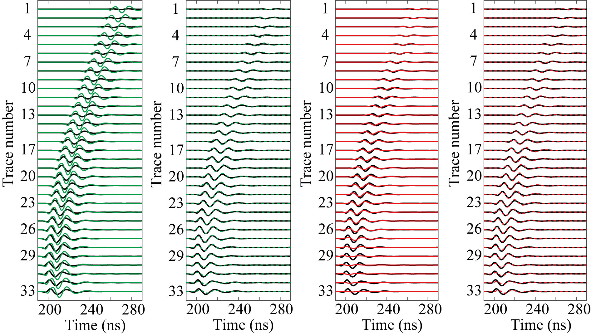
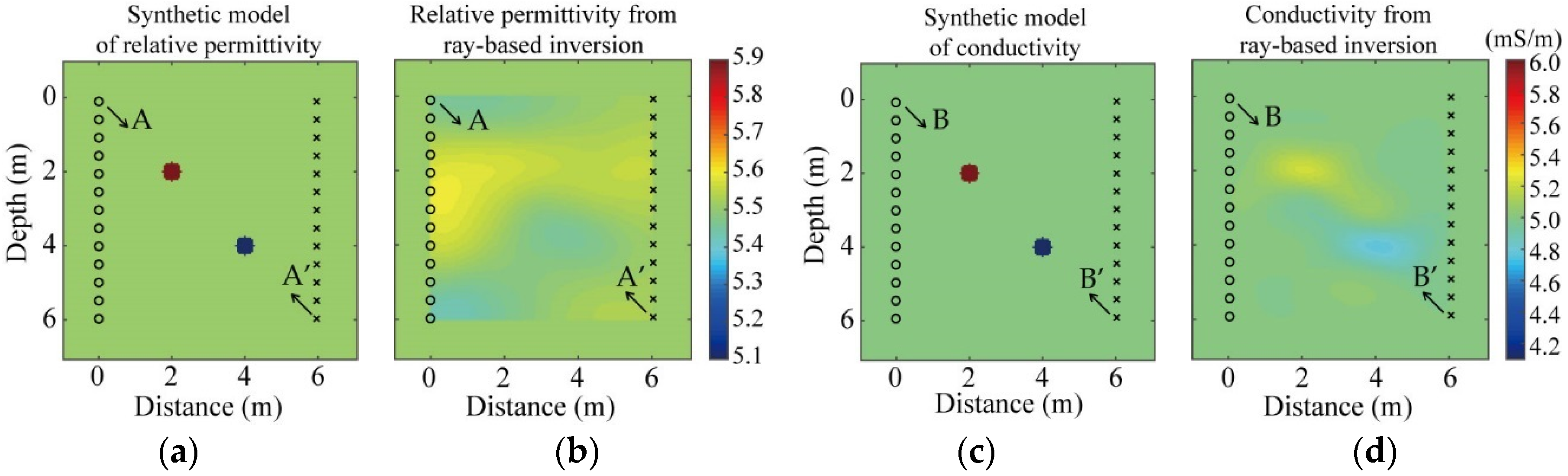
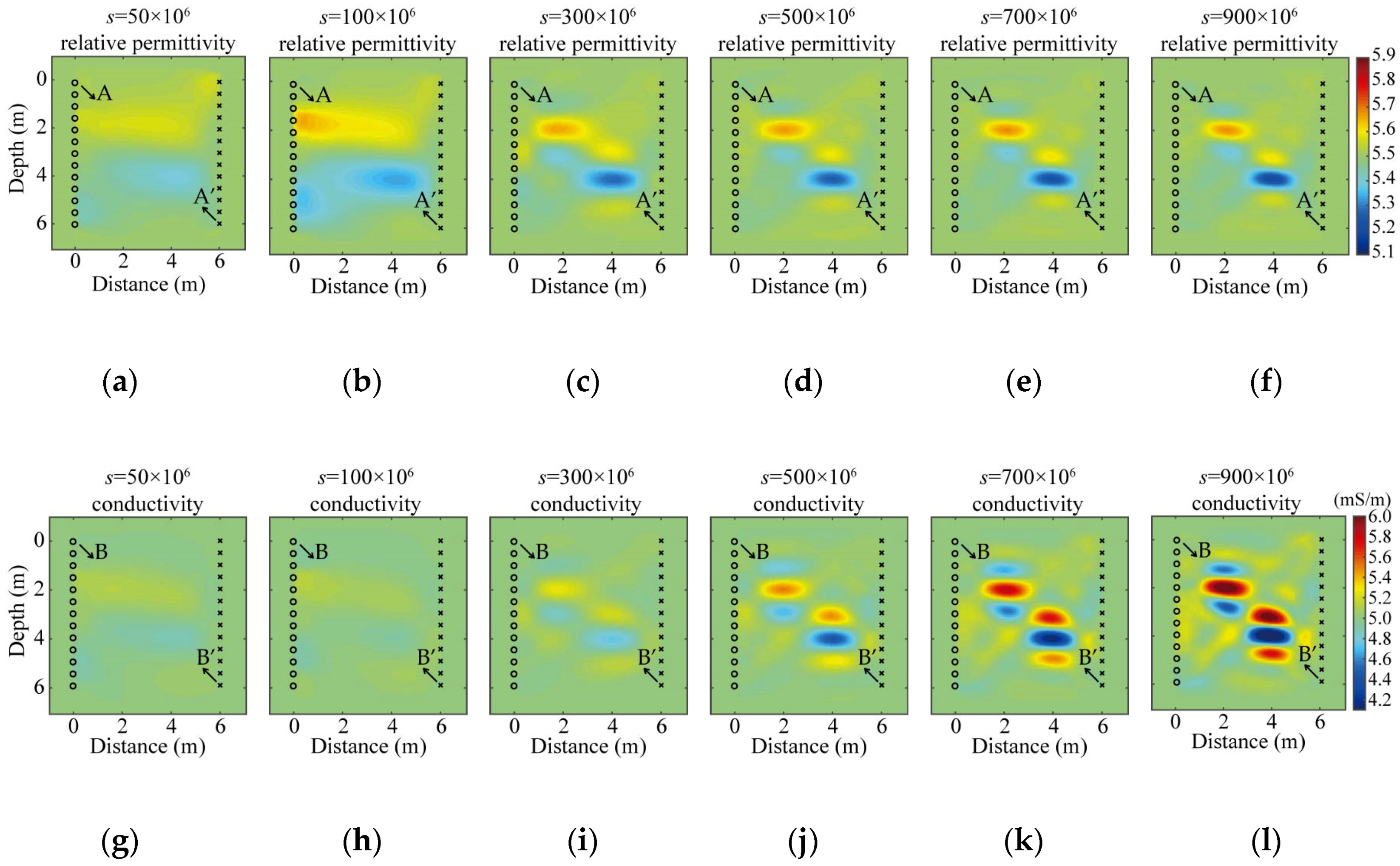
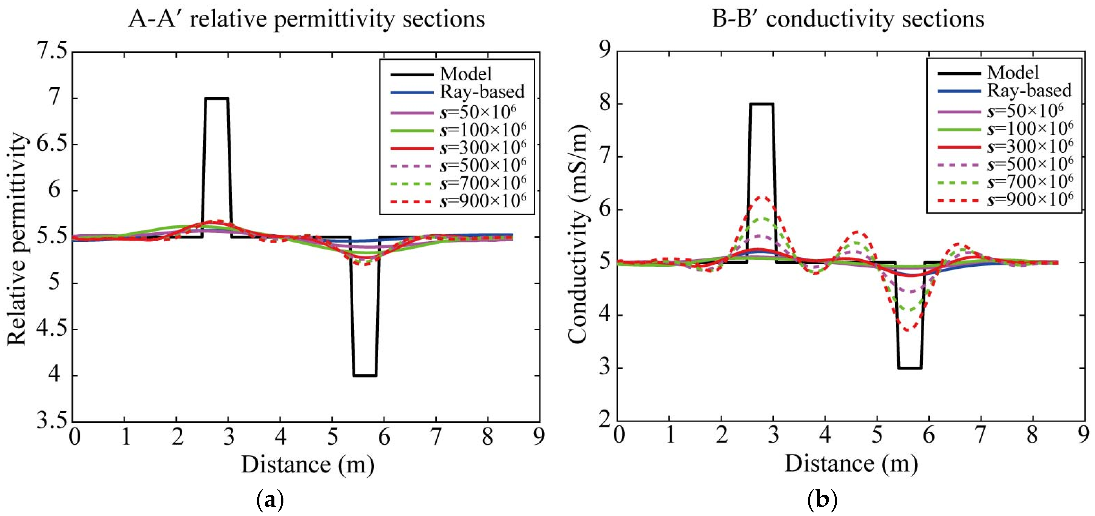
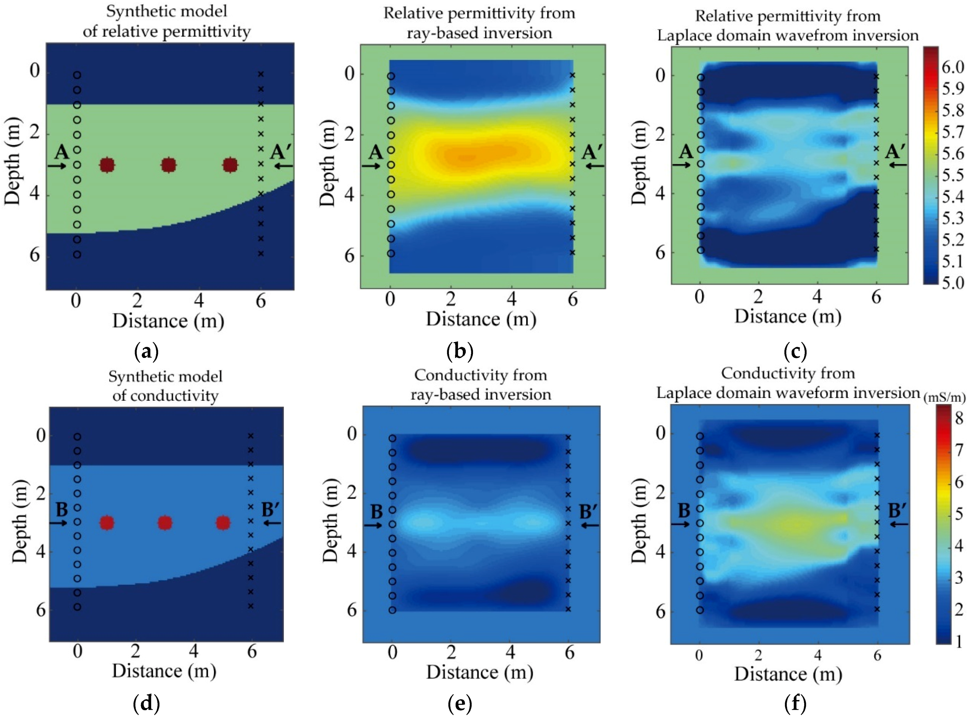
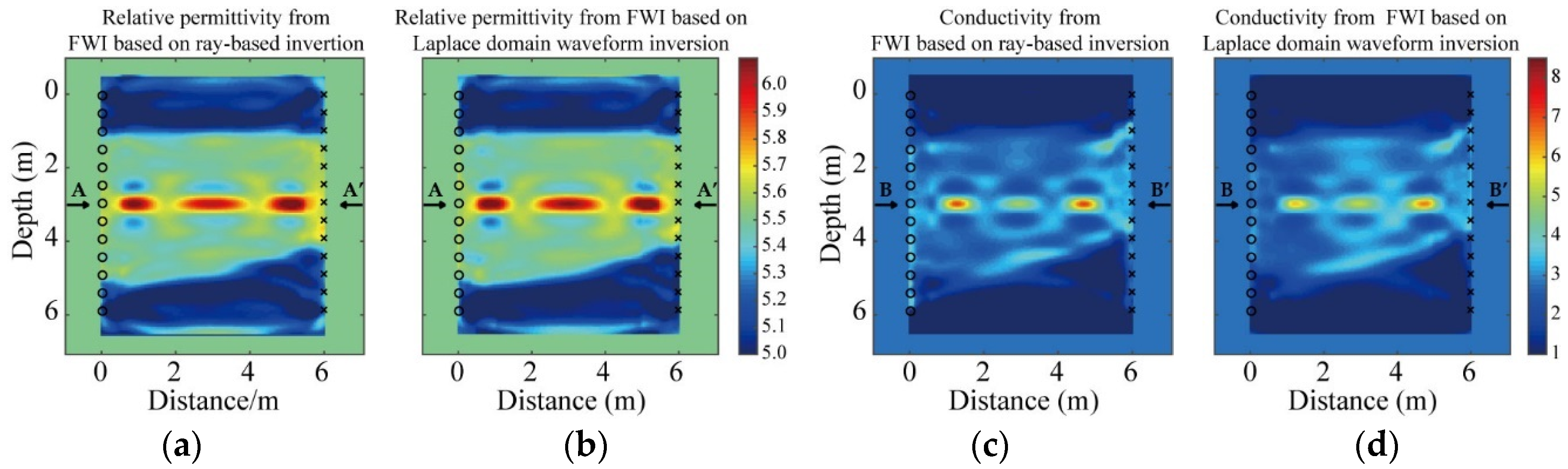
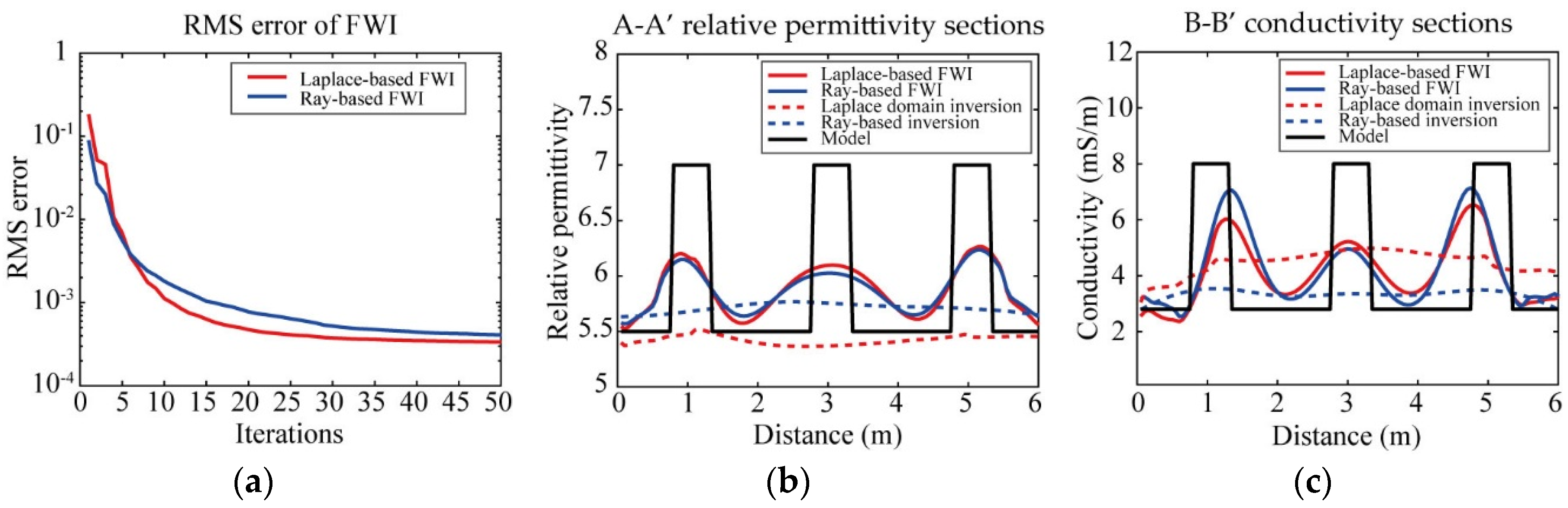
3.1. Synthetic Data 1: A Simple Model

Figure 1a,c show the permittivity and conductivity models for testing the performance of our Laplace domain waveform inversion. The model size was 6 m in both the horizontal and vertical directions. Two cylindrical anomalies with diameters of 0.5 m were placed in the homogeneous medium of relative permittivity ε r = 5.5 and conductivity σ = 0.005 S/m. The upper left anomaly was located at the position of (2 m, 2 m), and had a relative permittivity of 7 and conductivity of 0.008 S/m; the relative permittivity and conductivity of the lower right anomaly at the position of (4 m, 4 m) were 4 and 0.003 S/m, respectively. The two 6 m deep boreholes were 6 m apart. Thirteen transmitter positions (circle indicated) were spaced at 0.5 m intervals in the left borehole and thirteen receiver positions (crosses indicated) were spaced at 0.5 m in the right borehole (Figure 1).
The initial models in the ray-based inversion and Laplace domain waveform inversion have the same relative permittivity and conductivity values as the background medium of the true models. To weaken the near-field effect in the forward and backward modeling, a median filter [35] was applied near the source regions [18]. We used a stepped parameter updating approach because of the large gradient differences between the permittivity and conductivity. The permittivity was inverted with the fixed conductivity and then the conductivity was inverted with the fixed permittivity [14]. In the inversion process, the relative permittivity and conductivity are updated in the logarithmic domain to ensure their positive values and improve convergence [36].
Figure 1b,d are the inverted results of the ray-based inversion in which the two cylindrical anomalies cannot be distinguished because the diameter of the anomalies is smaller than the resolution of the ray-based method [6,7]. Figure 2 shows the results of Laplace domain waveform inversion at six different damping constants after 50 iterations. The two anomalies are well reconstructed when the Laplace domain waveform inversion is performed. However, the inverted results are smoother than the true models due to the long-wavelength features in the Laplace domain. The sizes of the reconstructed anomalies in Figure 2 are larger than those of results from the time domain FWI [18].
In Figure 2a,b,g,h, the results of Laplace domain waveform inversion at the low damping constants of s = 50 × 106 and s = 100 × 106 fail to reconstruct the shape of the cylindrical anomalies. This is due to the inaccuracy of the numerical Laplace transform of the time domain wavefield at a low damping constant [20]. When the damping constant is 300 × 106, both the results of relativity permittivity and conductivity reconstruct the two anomalies (Figure 2c,i). In the results of the Laplace domain waveform inversion at s = 500 × 106, 700 × 106 and 900 × 106 (Figure 2d–f,j–l), the two cylindrical anomalies are well reconstructed. The oscillations in Figure 2 are caused by the high wave-number updates in the models, and the high wave-number components dominate the wave-number information as the s values are increasing.
Figure 3 shows cross sections of the relative permittivity and conductivity through the results obtained by the ray-based inversion, Laplace domain waveform inversion, and the true models. In the results of the ray-based inversion and Laplace domain waveform inversion at damping constants of s = 50 × 106 and 100 × 106, the positions and sizes of the anomalies are not well reconstructed. When the damping constants are 300 × 106, 500 × 106, 700 × 106 and 900 × 106, the permittivity tomograms from the Laplace domain waveform inversion successfully reconstruct the positions of anomalies at a smooth scale (Figure 3a). Similar to the relative permittivity, the conductivity tomograms of the Laplace domain waveform inversion at high damping constants (s = 300 × 106, 500 × 106, 700 × 106 and 900 × 106) depict the positions of the anomalies well (Figure 3b). As the damping constant increases, the conductivity values of the anomalies are more accurate. This may be because the Laplace domain wavefield at high damping constants has higher contrast gradients than that at low damping constants [20]. However, the higher the Laplace damping constant, the less the damped wavefield contains the time domain wavefield. In addition, the damped wavefield at high damping constants is very easily disturbed by noise [20]. Therefore, the damping constant in the Laplace waveform inversion of cross-hole radar data should be chosen in a moderate range. We propose that approximately five times the value of the dominant frequency of the radar data is appropriate.
Laplace domain wavefields at different damping constants are also the zero frequency component of the damped wavefield, but at different values. The inverted results of relative permittivity are approximately the same. Since the first direct event always dominates the damped wavefield of the cross-hole radar data, multiple damping constants in the inversion would not help if an optimal damping constant is chosen. In this study, we used a single damping constant in our Laplace domain waveform inversion.

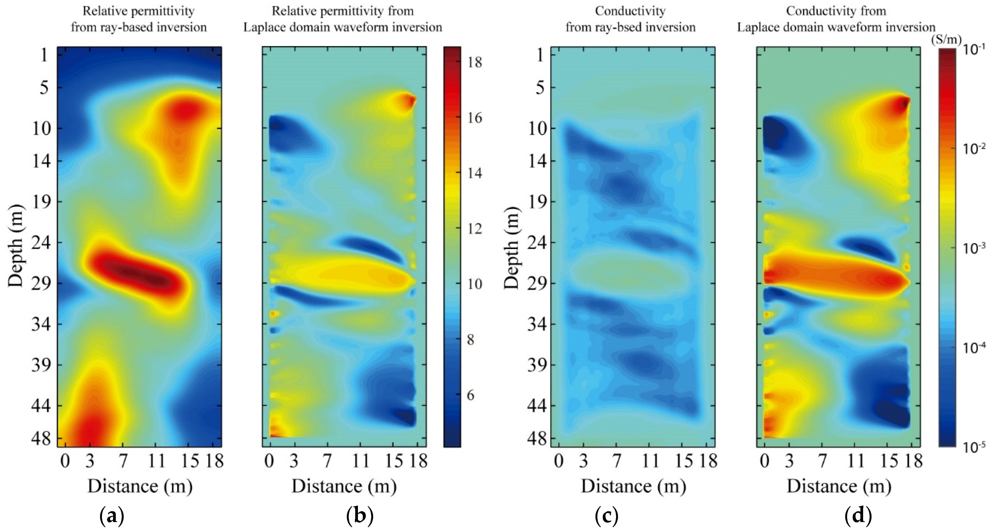
3.2. Synthetic Data 2: A Complex Model

To further check the performance of the Laplace domain waveform inversion, we built a three-layered model containing three cylindrical anomalies (Figure 4a,d). The horizontal and vertical sizes of the model were 6 m. The three anomalies with diameters of 0.5 m were placed at the positions of (1 m, 3 m), (3 m, 3 m) and (5 m, 3 m). The top layer and the bottom layer had the same relative permittivity of 5 and conductivity of 0.001 S/m. The three cylindrical anomalies of ε r = 7 and σ = 0.008 S/m were buried in the middle layer of ε r = 5.5 and σ = 0.0028 S/m. The initial models in the Laplace domain waveform inversion were the same as the middle layer. The locations of transmitters and receivers were the same as the simple example. In this example, the damping constant was 500 × 106 for the Laplace domain waveform inversion.
Figure 4 shows the relative permittivity and conductivity tomograms that result from the ray-based inversion and Laplace domain waveform inversion. The reconstructed anomalies in both relative permittivity and conductivity tomograms from the ray-based results (Figure 4b,e) are mixed together, whereas the layered medium is delineated roughly. In the results of the Laplace domain waveform inversion, the layer interfaces are well reconstructed (Figure 4c,f). However, the three anomalies in Figure 4c,f cannot be distinguished in the horizontal direction because of the small interval between the anomalies. To further compare the results of the ray-based inversion and Laplace domain waveform inversion, we apply their results as the initial models in the time domain FWI [18], and then compare their performance.
Figure 5a,c show the results of the time domain FWI based on the ray-based results, and Figure 5b,d are the results of the time domain FWI based on the Laplace domain waveform results. For both relative permittivity and conductivity, the layered medium and three cylindrical anomalies are rebuilt well. The interface between the middle layer and the bottom layer in Figure 5 agrees with that in the true model.
Figure 6a displays the curves of object function values during the 50 iterations of the time domain FWI in Figure 5. We note that the time domain FWI based on the Laplace domain waveform inversion has slightly large errors in the first five iterations, after which the error curve (red line in Figure 6a) decreases quickly and finally reach convergence at a lower value than the error curve (blue line in Figure 6a) of the time domain FWI based on the ray-based inversion. Figure 6b,c show cross-sections of relative permittivity and conductivity through the tomograms in Figure 4 and Figure 5. In the results of the time domain FWI, the positions and values of the cylindrical anomalies are clearly depicted. The relative permittivity values from the Laplace-based FWI are more accurate than those from the ray-based FWI (Figure 6b). In Figure 6c, FWI based on the ray-based inversion provides better values for the left and right anomalies. For the middle anomaly in Figure 6c, we note that the FWI based on the Laplace domain waveform inversion performs better. Similar to the results shown in Figure 3, inverted results of conductivity perform better than those of relative permittivity, as shown in previous studies [15,16,18]. In this example, Laplace domain waveform inversion is slightly better than the ray-based inversion to provide initial models for the time domain FWI.

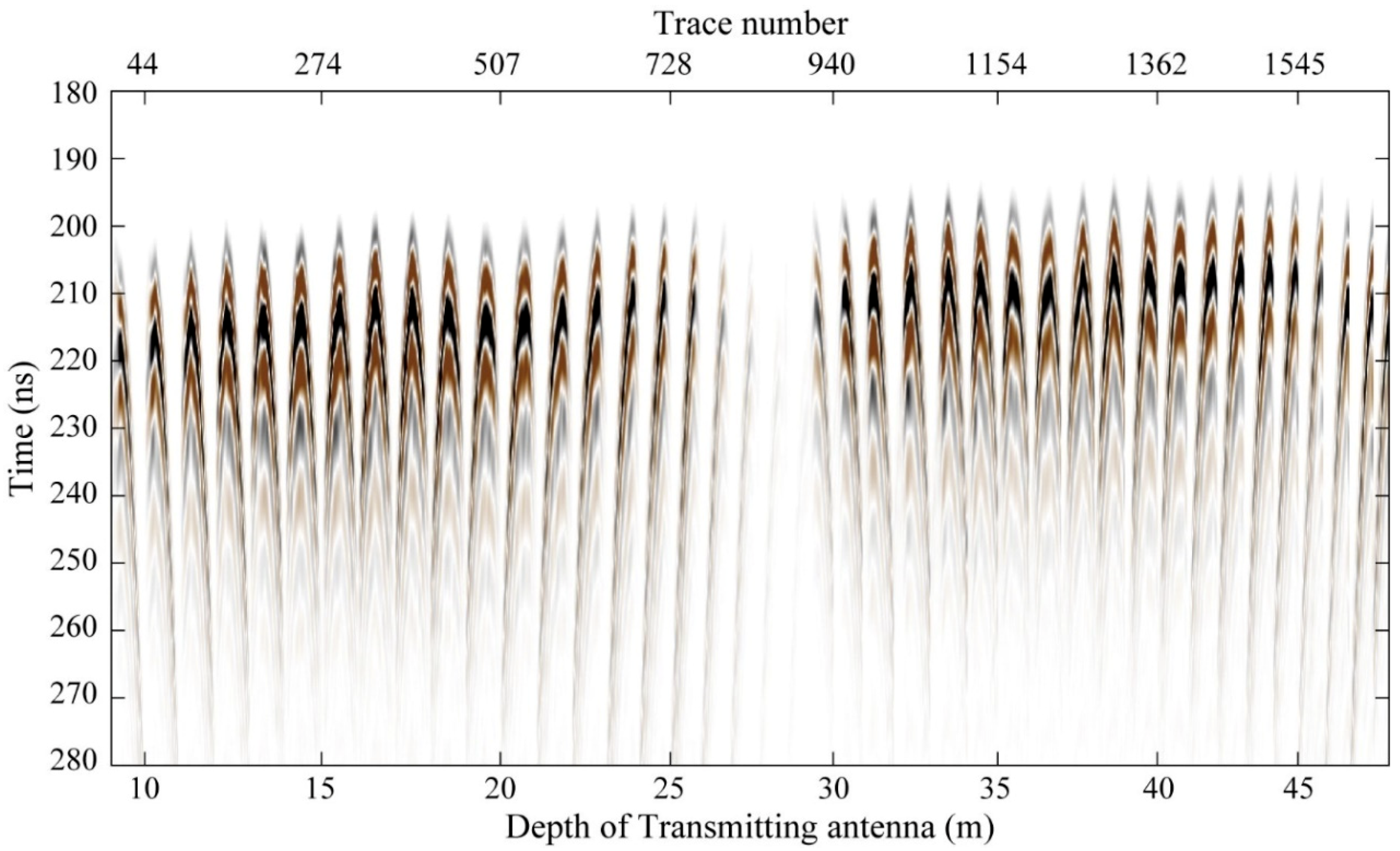
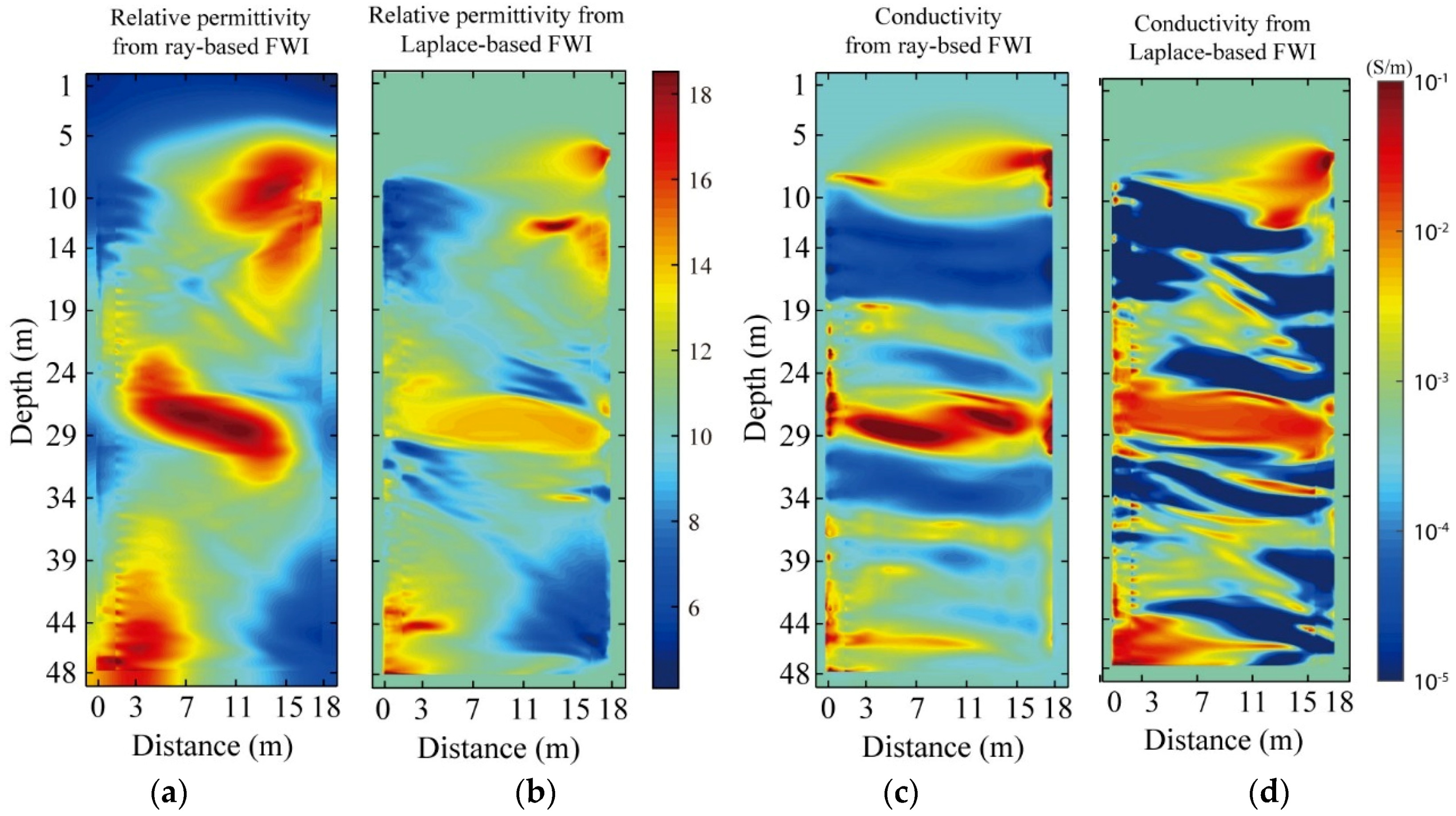
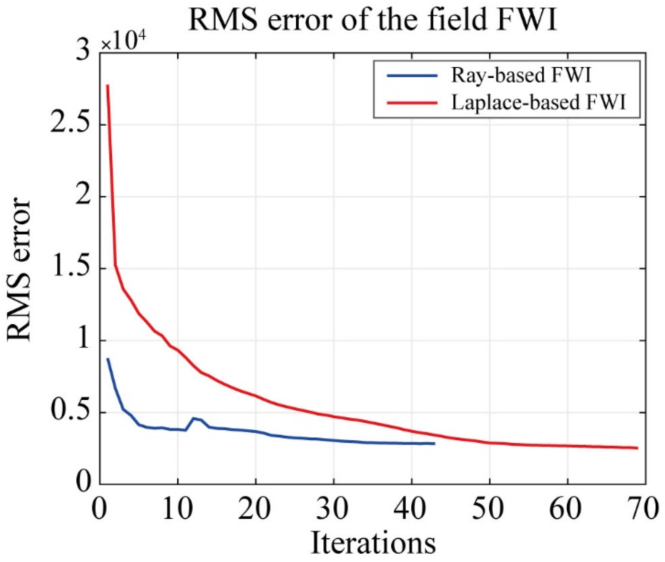
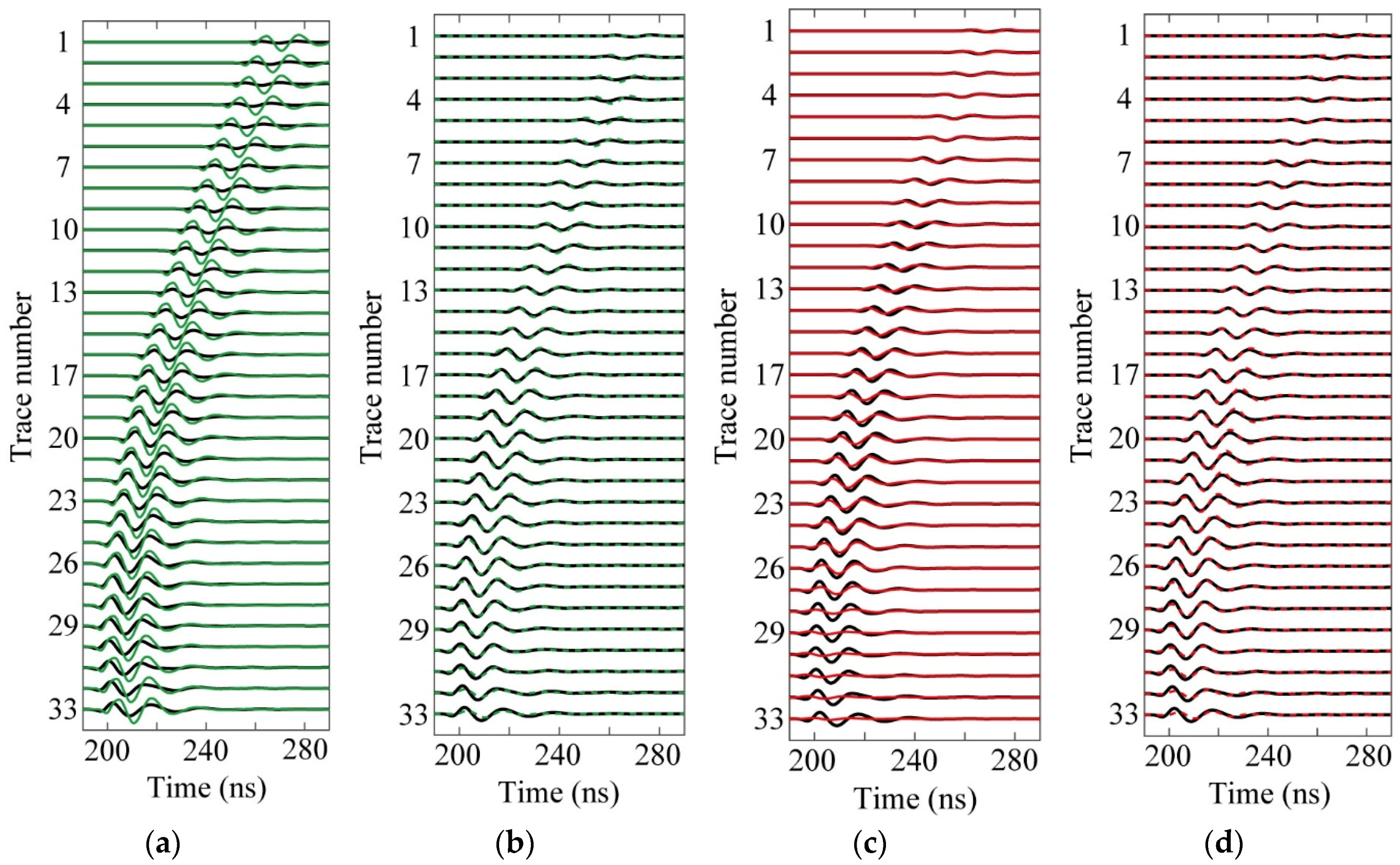
3.3. Field Data Measured at Guizhou

Field data were collected in the Guizhou Province using radar systems (MALA Geoscience) with 100 MHz borehole antennas. The horizontal distance between the two boreholes was 18 m. Forty source positions with 1 m intervals were placed between depths of 9 m and 48 m. The receiver positions corresponding to each source position were different (Table A1). The interval of receiver positions was 0.5 m. The raw data measured at the site is shown in Figure 7.
The estimation of source wavelet takes an important role in the waveform inversion of field data because the source wavelet must be known for forward modeling. However, the source wavelet is commonly unknown. We followed the deconvolution method proposed by Ernst et al. [15] to estimate the source wavelet, which has been presented in previous studies [15,18].
Before starting Laplace domain waveform inversion, the field data was subjected to careful preprocessing to improve the signal-to-noise ratio (SNR), including removal of the direct-current (DC) and band-pass (BP) filtering. In addition, careful muting of the signals before the first arrival event is needed due to the characteristics of the Laplace domain wavefield [20]. The dominant frequency of the field data is approximately 50 MHz due to the water-saturated environment. Based on the conclusion presented in Section 3.1, we chose 200 × 106, which is approximately four times larger than the dominant frequency of the field data, as the damping constant in the Laplace domain waveform inversion.
Figure 8a,c show the inverted results of the ray-based inversion and Figure 8b,d show the results of the Laplace domain waveform inversion after 83 iterations. From Figure 8a,b, we find that the relative permittivity tomograms from the ray-based inversion and Laplace domain waveform inversion are similar. A tunnel or cave exists at a depth of ~25 m and runs through the two boreholes. The upper right and bottom left regions have high permittivity values, whereas the permittivity of the upper left and bottom right regions is low (Figure 8a,b). However, the conductivity from the ray-based inversion (Figure 8c) shows low values (<10−3), which are probably unrealistic due to the existence of underground water. The reason is that the ray-based inversion can only provide relative spatial distributions of conductivity [7]. Conductivity results from the Laplace domain waveform inversion are significantly improved compared with that from the ray-based inversion.
Figure 9 shows the results of the time domain FWI by using the initial models from both ray-based inversion and Laplace domain waveform inversion. Figure 10 shows the root mean square (RMS) error curves of the field inversions with the ray-based (blue) and Laplace-based (red) results as the initial models. The convergence curves of the ray-based FWI and Laplace-based FWI stop after 43 and 69 iterations, respectively. The increase at the 12th iteration in the RMS curve of the ray-based FWI is caused by an additional source estimation during the inversion. We find that the Laplace-based FWI converges to a little lower value than the ray-based FWI. Compared to the initial models, we find obvious improvements in the results of the time domain FWI in Figure 9. At the depth of ~20 m, ~36 m and ~45 m, conductivity tomograms show horizontal layers with high values. We note that the tomograms from the Laplace-based FWI reveal more details than that from the ray-based FWI, especially for the conductivity tomograms. Figure 11 shows the predicted receiver gathers based on the inverted results for the 36th source position. Figure 11a,c are the predicted waveforms using the ray-based and Laplace domain waveform results. Though different initial models are used, waveforms of radar traces generated from the two FWI results agree well with the field waveforms (Figure 11b,d). The comparisons of waveforms indicate that inversions using both ray-based and Laplace domain waveform results are successful in the time domain. Initial models from the Laplace domain waveform inversion improve their corresponding results of FWI with more details (Figure 9b,d).

4. Discussion

FWI has been applied to interpret GPR data for approximately 20 years [13,14,15,16,17,18]. However, building accurate initial models is a challenge in the development of FWI. This is because the gradient-based FWI easily falls into local minima due to high nonlinearity. Accurate initial models are needed for FWI to overcome local minima to find the global minima. The traditional method to obtain initial models for GPR FWI is ray-based inversion, such as the first arrival time method [6] and the centroid frequency downshift method [7]. The first arrival time method can provide smooth distributions of relative permittivity, which requires accurate picking of first arrival times. However, the centroid frequency downshift method can only provide relative spatial distributions of conductivity [7]. Waveform inversion in the Laplace domain show a small advantage on permittivity tomograms because the travel time inversion is a well-established technology. More importantly, the Laplace domain waveform inversion can provide an improved distribution of conductivity, which contributes to the improvement in the time domain FWI.
Due to the characteristic of the Laplace domain wavefields, noise is amplified with the damping constants. Fortunately for cross-hole radar data, Laplace domain waveform inversion at a moderate damping constant, which is less sensitive to noise, is enough to provide initial models for the conventional FWI. Waveform inversion in the Laplace domain is robust because only a small portion of information about the data is used in the inversion. In addition, there is no need to extract first arrival times and amplitudes in the Laplace domain waveform inversion, making it less artificial intervention than the ray-based inversion. Therefore, the Laplace domain waveform algorithm has potential in the development of GPR FWI.

5. Conclusions

We successfully applied Laplace domain waveform inversion to synthetic and field cross-hole radar data. For the Laplace domain waveform inversion, the algorithm was derived via the derivation of Maxwell’s equation and a logarithmic object function. In the inversion, permittivity and conductivity can be obtained together by using a stepped updating strategy. The choice of damping constant in the inversion is investigated using a simple synthetic model. It is shown that the optimum value of the damping constant is approximately five times the value of the dominant frequency of radar data. Results of the time domain FWI based initial models from the ray-based inversion and Laplace domain waveform inversion indicate that the Laplace domain waveform inversion performs well. In the end, we applied the algorithm to a cross-hole field data. In the results of the field data, the permittivity and conductivity distributions from the time domain FWI using both ray-based and Laplace domain waveform results are comparable. Waveform inversion in the Laplace domain is an alternative algorithm to provide accurate initial models for GPR FWI.

Author Contributions

Methodology, X.M.; Software, X.M.; Formal analysis, S.L., L.F. and X.M.; Validation, Y.X.; Writing, X.M. and S.L.

Funding

This research was funded by the Science and Technology Development Fund, Macau SAR (File no. 0089/2018/A3, 119/2017/A3 & 008/2017/AFJ), the National Key Research and Development Program of China (2016YFC0600505), and the National Natural Science Foundation of China (Grant 41574109 & 41504085).

Acknowledgments

We thank Lanbo Liu from the University of Connecticut for providing the code for the ray-based method.

Conflicts of Interest

The authors declare no conflict of interest. The funders had no role in the design of the study; in the collection, analyses, or interpretation of data; in the writing of the manuscript, or in the decision to publish the results.

Appendix A

Table A1. Structures of field data.
Source IndexSource Position (m)Traces NumberFirst Receiver Position (m)Final Receiver Position (m)
1943829
210457.529.5
31146729.5
41245729
513466.529
614486.530
715476.529.5
81646729.5
917476.529.5
101846729.5
111947730
122047730
1321467.530
1422448.530
152343829
162441929
1725391029
18263810.529
1927381230.5
2028361330.5
2129611444
2230372644
23314126.546.5
24324723.546.5
2533492347
2634402746.5
2735402746.5
28364225.546
29374325.546.5
3038402746.5
3139432546
32403827.546
3341392746
3442362946.5
35433728.546.5
36443330.546.5
37453330.546.5
38463330.546.5
39473131.546.5
4048223646.5

References

  1. Daniels, D.J. Ground Penetrating Radar, 2nd ed.; The Institution of Engineering and Technology: London, UK, 2004. [Google Scholar]
  2. Olsson, O.; Falk, L.; Forslund, O.; Lundmark, L. Borehole radar applied to the characterization of hydraulically conductivity fracture-zones in crystalline rock. Geophys. Prospect. 1992, 40, 109–142. [Google Scholar] [CrossRef]
  3. Fullagar, P.K.; Livelybrooks, D.W.; Zhang, P.; Calvert, A.J.; Wu, Y. Radio tomography and borehole radar delineation of the McConnell nickel sulfide deposit, Sudbury, Ontario, Canada. Geophysics 2000, 65, 1920–1930. [Google Scholar] [CrossRef] [Green Version]
  4. Irving, J.D.; Knight, R.J. Effect of antennas on velocity estimates obtained from crosshole GPR data. Geophysics 2005, 70, K39–K42. [Google Scholar] [CrossRef] [Green Version]
  5. Wang, F.; Liu, S.X.; Qu, X.X. Crosshole radar traveltime tomographic inversion using the fast marching method and the iteratively linearized scheme. J. Environ. Eng. Geophys. 2014, 19, 229–237. [Google Scholar] [CrossRef]
  6. Zhang, J.; Toksoz, M.N. Nonlinear refraction traveltime tomography. Geophysics 1998, 63, 1496–1823. [Google Scholar] [CrossRef]
  7. Liu, L.; Lane, J.W.; Quan, Y. Radar attenuation tomography using the centroid frequency downshift method. J. Appl. Geophys. 1998, 40, 105–116. [Google Scholar] [CrossRef]
  8. Williamson, P.R. A guide to the limits of resolution imposed by scattering in ray tomography. Geophysics 1991, 56, 202–207. [Google Scholar] [CrossRef]
  9. Williamson, P.R.; Worthington, M.H. Resolution limits in ray tomography due to wave behavior—Numerical experiments. Geophysics 1993, 58, 727–735. [Google Scholar] [CrossRef]
  10. Tarantola, A.; Valette, B. Generalized no-linear inverse problems solved using the least-squares criterion. Rev. Geophys. 1982, 20, 219–232. [Google Scholar] [CrossRef]
  11. Devaney, A.J. Geophysical diffraction tomography. IEEE Trans. Geosci. Remote Sens. 1984, GE-22, 3–13. [Google Scholar] [CrossRef]
  12. Reiter, D.T.; Rodi, W. Nonlinear waveform tomography applied to crosshole seismic data. Geophysics 1996, 61, 902–913. [Google Scholar] [CrossRef]
  13. Kuroda, S.; Takeuchi, M.; Kim, H.J. Full waveform inversion algorithm for interpreting cross-borehole GPR data. In Proceedings of the 2005 SEG Annual Meeting, Houston, TX, USA, 6–11 November 2005; pp. 1176–1179. [Google Scholar]
  14. Ernst, J.R.; Green, A.G.; Maurer, H.; Holliger, K. Application of a new 2D time-domain full-waveform inversion scheme to crosshole radar data. Geophysics 2007, 72, J53–J64. [Google Scholar] [CrossRef]
  15. Ernst, J.R.; Maurer, H.; Green, A.G.; Holliger, K. Full-waveform inversion of crosshole radar data based on 2-D finite-difference time-domain solutions of Maxwell’s equations. IEEE Trans. Geosci. Remote Sens. 2007, 45, 2807–2828. [Google Scholar] [CrossRef]
  16. Meles, G.A.; Kruk, J.V.D.; van der Kruk, J.; Greenhalgh, S.A.; Ernst, J.R.; Maurer, H.; Green, A.G. A new vector waveform inversion algorithm for simultaneous updating of conductivity and permittivity parameters from combination crosshole/borehole-to-surface GPR data. IEEE Trans. Geosci. Remote Sens. 2010, 48, 3391–3407. [Google Scholar] [CrossRef]
  17. Belina, F.A.; Irving, J.; Ernst, J.R.; Holliger, K. Waveform inversion of crosshole georadar data: Influence of source wavelet variability and the suitability of a single wavelet assumption. IEEE Trans. Geosci. Remote Sens. 2012, 50, 4610–4625. [Google Scholar] [CrossRef]
  18. Liu, S.; Liu, X.; Meng, X.; Fu, L.; Lu, Q.; Deng, L. Application of time-domain full waveform inversion to cross-hole radar data measured at Xiuyan Jade Mine, China. Sensors 2018, 18, 3114. [Google Scholar] [CrossRef] [PubMed]
  19. Virieux, J.; Operto, S. An overview of full-waveform inversion in exploration geophysics. Geophysics 2009, 74, WCC127–WCC152. [Google Scholar] [CrossRef]
  20. Shin, C.; Cha, Y.H. Waveform inversion in the Laplace domain. Geophys. J. Int. 2008, 173, 922–931. [Google Scholar] [CrossRef] [Green Version]
  21. Ha, W.; Shin, C. Why do Laplace-domain waveform inversions yield long-wavelength results? Geophysics 2013, 78, R167–R173. [Google Scholar] [CrossRef]
  22. Shin, C.; Ha, W. A comparison between the behavior of objective functions for waveform inversion in the frequency and Laplace domains. Geophysics 2008, 73, VE119–VE133. [Google Scholar] [CrossRef]
  23. Shin, C.; Cha, Y. Waveform inversion in the Laplace-Fourier domain. Geophys. J. Int. 2009, 177, 1067–1079. [Google Scholar] [CrossRef]
  24. Ha, W.; Shin, C. Laplace-domain full-waveform inversion of seismic data lacking low-frequency information. Geophysics 2012, 77, R199–R206. [Google Scholar] [CrossRef]
  25. Park, E.; Ha, W.; Chung, W.; Shin, C.; Min, D.-J. 2D Laplace-domain waveform inversion of field data using a power objective function. Pure Appl. Geophys. 2013, 170, 2075–2085. [Google Scholar] [CrossRef]
  26. Yoon, B.J.; Ha, W.; Son, W.; Shin, C.; Calandra, H. 3D acoustic modelling and waveform inversion in the Laplace domain for an irregular sea floor using the Gaussian quadrature integration method. J. Appl. Geophys. 2012, 87, 107–117. [Google Scholar] [CrossRef]
  27. Kim, Y.; Shin, C.; Calandra, H.; Min, D.-J. An algorithm for 3D acoustic time-Laplace-Fourier-domain hybrid full waveform inversion. Geophysics 2013, 78, R151–R166. [Google Scholar] [CrossRef]
  28. Shin, J.; Ha, W.; Jun, H.; Min, D.-J.; Shin, C. 3D Laplace-domain full waveform inversion using a single GPU card. Comput. Geosci. 2014, 67, 1–13. [Google Scholar] [CrossRef]
  29. Ha, W.; Kang, S.-G.; Shin, C. 3D Laplace-domain waveform inversion using a low-frequency time-domain modeling algorithm. Geophysics 2015, 80, R1–R13. [Google Scholar] [CrossRef]
  30. Son, W.; Pyun, S.; Shin, C.; Kim, H.-J. Laplace-domain wave-equation modeling and full waveform inversion in 3D isotropic elastic media. J. Appl. Geophys. 2014, 105, 120–132. [Google Scholar] [CrossRef]
  31. Roden, J.A.; Gedney, S.D. Convolution PML (CPML): An efficient FDTD implementation of the CFS-PML for arbitrary media. Microw. Opt. Technol. Lett. 2000, 27, 334–339. [Google Scholar] [CrossRef]
  32. Shin, C.; Min, D.-J. Waveform inversion using a logarithmic wavefield. Geophysics 2006, 71, R31–R42. [Google Scholar] [CrossRef] [Green Version]
  33. Pica, A.; Diet, J.P.; Tarantola, A. Nonlinear inversion of seismic reflection data in a laterally invariant medium. Geophysics 1990, 55, 284–292. [Google Scholar] [CrossRef]
  34. Kryzhniy, V.V. Numerical inversion of the Laplace transform: Analysis via regularized analytic continuation. Inverse Probl. 2006, 22, 579–597. [Google Scholar] [CrossRef]
  35. Tukey, J.W. Exploratory Data Analysis; Addison Wesley: Massachusetts, MA, USA, 1977. [Google Scholar]
  36. Tarantola, A. Inverse Problem Theory and Methods for Model Parameter Estimation; Society for Industrial and Applied Mathematics: Philadelphia, PA, USA, 2005. [Google Scholar]
Figure 1. A simple model with two cylindrical anomalies buried in a homogeneous medium. (a) Relative permittivity and (c) conductivity of the model; (b) relative permittivity and (d) conductivity tomograms from the ray-based results.
Remotesensing 11 01839 g001
Figure 2. Permittivity and conductivity tomograms from the Laplace domain waveform inversion. (a,g) at s = 50 × 106; (b,h) at s = 100 × 106; (c,i) at s = 300 × 106; (d,j) at s = 500 × 106; (e,k) at s = 700 × 106; (f,l) at s = 900 × 106.
Remotesensing 11 01839 g002
Figure 3. Comparisons among the inverted tomograms from the ray-based inversion, Laplace domain waveform inversion, and the true models. (a) Relative permittivity along section A-A’; (b) conductivity along section B-B’.
Remotesensing 11 01839 g003
Figure 4. A three-layered model with three cylindrical anomalies buried in the middle layer. (a) Relative permittivity and (d) conductivity of the model; (b) relative permittivity and (e) conductivity tomograms from the ray-based results; (c) relative permittivity and (f) conductivity tomograms from the Laplace domain waveform results.
Remotesensing 11 01839 g004
Figure 5. Tomograms from the time domain full waveform inversion (FWI). (a) Relative permittivity and (c) conductivity based on initial models from the ray-based inversion; (b) relative permittivity and (d) conductivity based on initial models from the Laplace domain waveform inversion.
Remotesensing 11 01839 g005
Figure 6. Comparisons among the time domain full waveform inverted results based on the ray-based and Laplace domain waveform inversion. (a) Root mean square (RMS) error curves; (b) relative permittivity along the A-A’ section and (c) conductivity along the B-B’ section.
Remotesensing 11 01839 g006
Figure 7. Measured cross-hole radar raw data in Guizhou Province.
Remotesensing 11 01839 g007
Figure 8. Tomograms of Guizhou field data. (a) Relative permittivity and (c) conductivity from the ray-based inversion; (b) relative permittivity and (d) conductivity from the Laplace domain waveform inversion.
Remotesensing 11 01839 g008
Figure 9. Tomograms of Guizhou field data from the time domain FWI. (a) Relative permittivity and (c) conductivity from the ray-based FWI; (b) relative permittivity and (d) conductivity from the Laplace-based FWI.
Remotesensing 11 01839 g009
Figure 10. RMS error curves in the time domain FWI of the field data.
Remotesensing 11 01839 g010
Figure 11. Waveform comparisons for receiver gathers at the depth of 44 m. The black lines correspond to the field radar traces. (a) The green lines are the predicted data generated from the ray-based results; (b) the dashed green lines are the predicted data generated from the ray-based FWI; (c) the red lines show the predicted traces generated from the Laplace domain waveform results; (d) the dashed red lines show the predicted traces generated from the Laplace-based FWI. Amplitudes in (ad) are normalized with respect to the maximum amplitude of the field data.
Remotesensing 11 01839 g011

