Article

Evaluating the Performance of Satellite-Derived Vegetation Indices for Estimating Gross Primary Productivity Using FLUXNET Observations across the Globe

1
Research Base of Karst Eco-environments at Nanchuan in Chongqing, Ministry of Nature Resources, School of Geographical Sciences, Southwest University, Chongqing 400715, China
2
Earth Systems Research Center, Institute for the Study of Earth, Oceans, and Space, University of New Hampshire, Durham, NH 03824, USA
3
Chongqing Engineering Research Center for Remote Sensing Big Data Application, School of Geographical Sciences, Southwest University, Chongqing 400715, China
*
Authors to whom correspondence should be addressed.
Remote Sens. 2019, 11(15), 1823; https://doi.org/10.3390/rs11151823
Submission received: 26 June 2019 / Revised: 25 July 2019 / Accepted: 1 August 2019 / Published: 4 August 2019

Abstract

:
Satellite-derived vegetation indices (VIs) have been widely used to approximate or estimate gross primary productivity (GPP). However, it remains unclear how the VI-GPP relationship varies with indices, biomes, timescales, and the bidirectional reflectance distribution function (BRDF) effect. We examined the relationship between VIs and GPP for 121 FLUXNET sites across the globe and assessed how the VI-GPP relationship varied among a variety of biomes at both monthly and annual timescales. We used three widely-used VIs: normalized difference vegetation index (NDVI), enhanced vegetation index (EVI), and 2-band EVI (EVI2) as well as a new VI - NIRV and used surface reflectance both with and without BRDF correction from the moderate resolution imaging spectroradiometer (MODIS) to calculate these indices. The resulting traditional (NDVI, EVI, EVI2, and NIRV) and BRDF-corrected (NDVIBRDF, EVIBRDF, EVI2BRDF, and NIRV, BRDF) VIs were used to examine the VI-GPP relationship. At the monthly scale, all VIs were moderate or strong predictors of GPP, and the BRDF correction improved their performance. EVI2BRDF and NIRV, BRDF had similar performance in capturing the variations in tower GPP as did the MODIS GPP product. The VIs explained lower variance in tower GPP at the annual scale than at the monthly scale. The BRDF-correction of surface reflectance did not improve the VI-GPP relationship at the annual scale. The VIs had similar capability in capturing the interannual variability in tower GPP as MODIS GPP. VIs were influenced by temperature and water stresses and were more sensitive to temperature stress than to water stress. VIs in combination with environmental factors could improve the prediction of GPP than VIs alone. Our findings can help us better understand how the VI-GPP relationship varies among indices, biomes, and timescales and how the BRDF effect influences the VI-GPP relationship.

Graphical Abstract

1. Introduction

Terrestrial gross primary productivity (GPP), the amount of carbon absorbed by terrestrial plants through photosynthesis, is the largest carbon flux between the terrestrial biosphere and the atmosphere. It also drives the terrestrial food chain and is the basis for agricultural and wood production. Quantifying GPP is therefore essential for assessing ecosystem carbon dynamics, climate feedbacks, agricultural productivity, and human welfare. Satellite-derived vegetation indices (VIs) are indicative of photosynthetic activity and have been widely used as proxies for GPP [1,2,3,4] or to directly estimate GPP [5,6,7]. Ground-based GPP data from the eddy covariance (EC) flux towers are typically used as reference data to evaluate the performance of satellite-derived VIs in approximating or estimating GPP. Better understanding the relationships between the VIs and GPP for a wide variety of biomes at various timescales is essential for assessing ecosystem functioning, vegetation productivity, and carbon budgets at regional to global scales using satellite-derived VIs.
The normalized difference vegetation index (NDVI) is perhaps the most widely used VI in satellite monitoring of vegetation productivity [8]. NDVI captures the contrast in reflectance between the red and NIR wavelengths and was first developed to estimate vegetation greenness [9]. It has been widely adopted as a proxy for GPP. For example, a close relationship between NDVI and GPP at the daily timescale was found for a maize cropland [10], a deciduous forest [11] and a pine forest [12]. However, NDVI is sensitive to soil background brightness and is influenced by soil texture and moisture conditions [13]; NDVI is also sensitive to scattering by the atmosphere from highly variable aerosols [14,15] and also tends to saturate in multi-layered and dense canopies [16,17]. The enhanced vegetation index (EVI) was proposed to reduce these limitations by using reflectance in the blue band to correct for effects of aerosols [17,18]. Many studies reported that EVI had a better performance in estimating GPP for alpine meadow [19], maize [20] and wetlands [21] than NDVI. An EVI-based index without the blue band - EVI2 was later developed [22]. EVI2 is similar to the 3-band EVI especially when atmospheric effects are insignificant and the reflectance data are in good quality [22]. Compared with NDVI, this 2-band index was shown to be able to better capture subtle changes in vegetation condition and structure and to have higher correlation with GPP for maize and soybean ecosystems [10,23] and a red pine forest [24]. EVI2 has also been shown to have a slightly higher correlation with GPP than did EVI in a forest ecosystem [25].
Although these satellite-derived VIs have been widely used to approximate or estimate GPP [5,6,7,8,26,27], it remains unclear how strongly the VIs are related to GPP and how the VI-GPP relationship varies across VIs, biomes, timescales, and different climatic conditions. Prior to December 2015, the FLUXNET database available to the research community was the La Thuile dataset released in 2007. The duration of the GPP data from this database had only up to four years of overlap with the NDVI record from the moderate resolution imaging spectroradiometer (MODIS), which hindered the analysis for the VI-GPP relationship at the annual scale. The NDVI record derived from the Advanced Very High Resolution Radiometer (AVHRR) has a longer overlap with the La Thule database, but there is large scale-mismatch between the flux tower footprint and the AVHRR grid cell (~64 km2). The new FLUXNET2015 dataset, released in December 2015, consists of EC and meteorological data for 221 flux towers across the globe. Compared with its predecessor, the La Thuile dataset, the FLUXNET2015 dataset had much longer temporal coverage with some sites spanning the period from the early 1990s to 2014. As a result, the overlap between the FLUXNET2015 dataset and MODIS data products is up to 15 years (2000–2014), which makes it feasible to examine the VI-GPP relationship at the annual scale.
Moreover, in most previous studies, satellite-derived VIs were calculated from surface reflectance that was not corrected with the bidirectional reflectance distribution function (BRDF). For a given ground object, the surface reflectance measured by satellites varies with changing illumination and viewing geometry (i.e., solar zenith angle, view zenith angle, and relative azimuth angle), leading to varying values in the resulting VIs [28]. The BRDF mathematically describes the surface reflectance as a function of sun-object-sensor geometry and can be used to standardize reflectance observations with varying sun-view geometries to a common standard geometry [29]. A large number of previous studies based on VIs (e.g., [8,27]) made use of the AVHRR NDVI record, while this NDVI dataset is derived from surface reflectance that was not corrected with BRDF. The MODIS-derived VIs used in many studies [7,30,31] were also based on surface reflectance (e.g., the MOD09 and MYD09 products) that was not corrected with BRDF. Some previous studies reported that VIs based on BRDF-corrected reflectance exhibited better performances than the traditional VIs (i.e., VIs based on surface reflectance not corrected with BRDF) [1,2]. For example, the BRDF-corrected NDVI and EVI had slightly stronger correlation with tower GPP than the traditional VIs. Recently, a new index based on BRDF-corrected reflectance, the near-infrared reflectance of vegetation (NIRV), was proposed [32]. NIRV is the product of the BRDF-corrected NIR reflectance and BRDF-corrected NDVI. NIRV represents the proportion of reflectance attributable to the vegetation from a physical perspective and has been shown to be better related to GPP than NDVI or NIR alone [32].
To our knowledge, no study has compared traditional VIs (i.e., VIs based on surface-reflectance that is not corrected with BRDF) against BRDF-corrected VIs for estimating GPP for a large number of sites across a wide variety of biomes at both seasonal and annual scales. The MODIS ASCII Subsets for BRDF-corrected surface reflectance products (e.g., MCD43A4) were not available until very recently. Prior the release of the Collection 6 MODIS ASCII Subsets in 2017, the MCD43A4 subsets for each EC site had to be extracted from entire MODIS tiles by the users, while extracting MODIS subsets for a large number of sites globally for multiple years is computationally intensive and time consuming. The recent release of the MCD43A4 subsets makes it feasible to extract BRDF-corrected surface reflectance and then to calculate BRDF-corrected VIs for a large number of sites in a timely fashion.
The recent concurrent availability of FLUXNET and MODIS data for a large number of sites over a 15-year period (2000–2014) and the recent availability of the MODIS ASCII subsets for BRDF-corrected surface reflectance products provide an unprecedented opportunity to examine the relationships between satellite-derived VIs (both traditional and BRDF-corrected VIs) and tower GPP across a wide variety of biomes at various timescales. Here we examined the relationships between VIs and tower GPP for a total of 121 EC sites across the globe and assessed how the VI-GPP relationship varied among various VIs and a wide variety of biomes and at both monthly and annual timescales. We used three widely-used VIs: NDVI, EVI, and EVI2 along the new index - NIRV, and used surface reflectance products both with and without BRDF correction to calculate these VIs. Besides these six VIs, the new VI based on BRDF-corrected reflectance - NIRV was also used. To evaluate the usefulness of the VIs for estimating GPP, we also assessed the relationship between the MODIS GPP product and flux tower GPP for these sites. We then investigated the correlations of VIs with temperature and water stresses to reveal how VIs respond to temperature and water availability. Finally, we examined how VIs in combination with environmental factors could better explain the variations in GPP. Our findings can reveal the performance of satellite-derived VIs for approximating GPP and the influence of the BRDF effect and informing future ecosystem functioning, vegetation productivity, and carbon cycle studies based on VIs.

2. Data and Methods

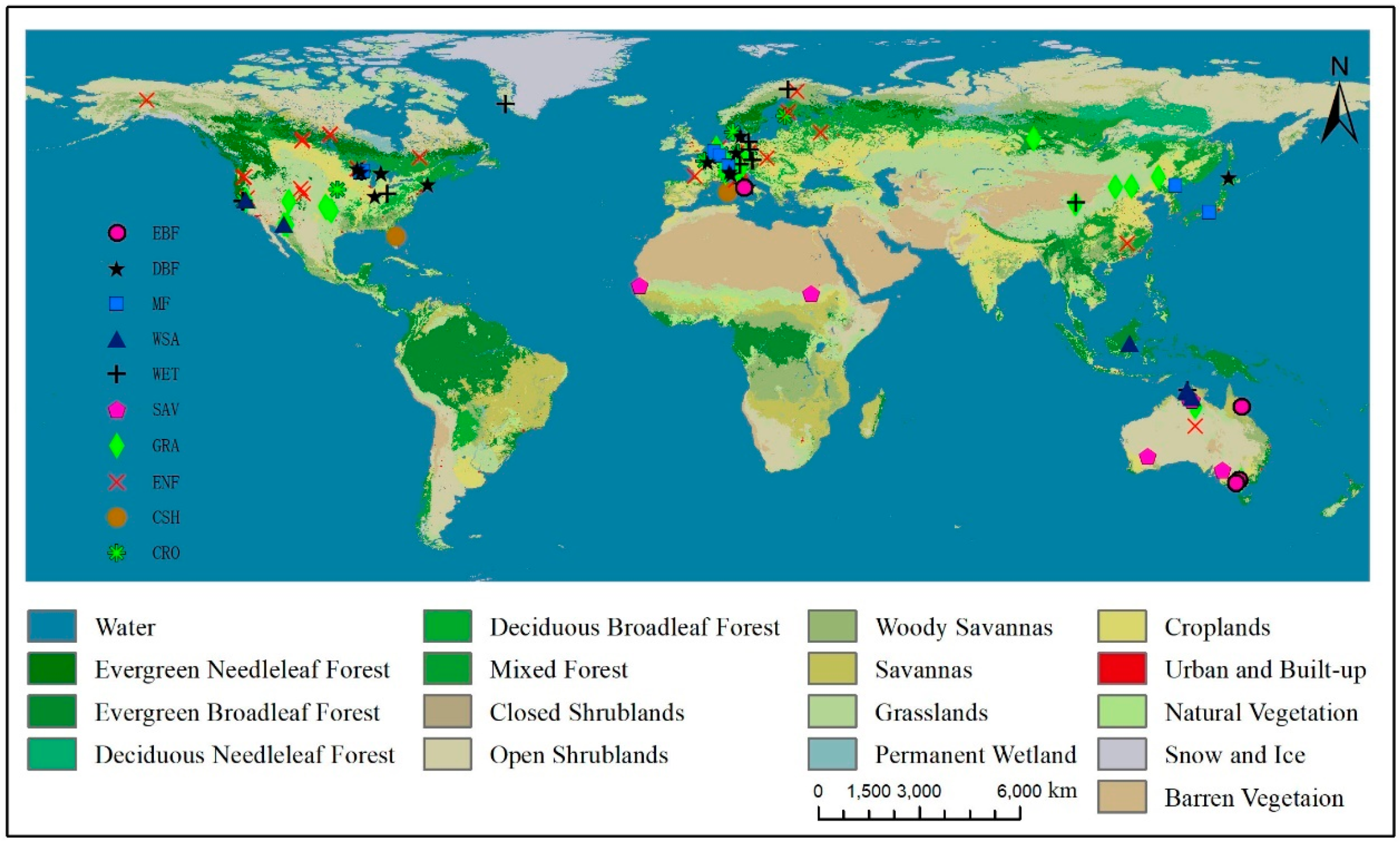
2.1. Study Sites and Flux Tower Data

We used flux and meteorological data from the latest FLUXNET synthesis dataset, the FLUXNET2015 database. This database was first released in December 2015 with more site-years of data added in 2016. It provides standardized and high-quality flux and meteorological data for a total of 221 sites across the globe (http://fluxnet.fluxdata.org/data/fluxnet2015-dataset/data-processing/). Over the past decade or so, there have been two major data synthesis activities initiated by the FLUXNET research community, leading to two synthesis datasets: La Thuile and FLUXNET2015. The FLUXNET2015 dataset has up to 15 years of overlap between EC data and MODIS data products, while the La Thuile dataset has only up to 5 years of overlap with the MODIS data record. The new dataset also has better quality than its predecessor. We therefore used the FLXUNET2015 dataset in our study. The flux and meteorological data in the dataset were gap filled, and the NEE measurements were partitioned into GPP and ecosystem respiration using standardized procedures [33].
In our study, we selected 121 Tier-1 sites that are open and free for scientific research (Figure 1). The site code, site name, latitude, longitude, vegetation type, and duration of measurements, and references are provided in Table S1. Although these sites are distributed across the globe with latitudinal distribution and encompass the following ten biomes: evergreen needleleaf forests (ENF), evergreen broadleaf forests (EBF), deciduous broadleaf forests (DBF), mixed forests (MF), closed and open shrublands (COSH), woody savannas (WSA), savannas (SAV), grasslands (GRA), wetlands (WET), and croplands (CRO), there are actually no significant latitudinal impacts on GPP and VIs (Figure S1). The GPP data (GPP-DT-CUT-REF) partitioned from NEE using the daytime partitioning approach [34] and meteorological data were used in our analysis.

2.2. Vegetation Indices (VIs)

We used the following four vegetation indices: NDVI, EVI, EVI2, and NIRV in this study. NDVI is perhaps the most widely used vegetation index. NDVI captures the difference between maximum reflection of radiation in the near-infrared band due to the leaf cellular structure and the maximum absorption of radiation in the red band due to the chlorophyll pigments. NDVI can be expressed as follows:
NDVI = N R N + R
where N and R are the reflectance in the near-infrared (NIR) and red bands, respectively. Although NDVI has been widely used to approximate photosynthetic activity, this index has some limitations. NDVI is sensitive to soil background brightness and is influenced by soil texture and moisture conditions [13].
To overcome the saturation effects of NDVI, weight factors were introduced to the NIR reflectance term in the NDVI formulation to adjust the relative contributions of the red and NIR reflectance. The resulting VI-EVI can be expressed as follows:
EVI = G N R N + C 1 R C 2 B + L
where B is the reflectance in blue band; G is a gain factor; C1 and C2 are the coefficients of the aerosol resistance term that are used to correct for aerosol affects in the red band with the blue band; L functions as the soil adjustment factor. The coefficients adopted in the EVI algorithm are as follows: G = 2.5, C1 = 6, C2 = 7.5 and L = 1. EVI has been widely used as proxies of vegetation productivity or to estimate GPP [35,36].
The visible bands are highly related with each other, and the blue reflectance can be expressed as a function of the red reflectance [37]. A two-band EVI index, EVI2, was developed assuming the blue-band reflectance is a function of the red-band reflectance (B = c*R) and using the L, C1 and C2 values in the EVI formula [22]. With the optimal C1, C2 and G values, EVI2 can be expressed as follows:
EVI 2 = 2.5 N R N + 2.4 R + 1
EVI2 not only gained its heritage from EVI but also improved the linearity with vegetation biophysical parameters [22].
A more recently developed index, NIRV, is the product of the BRDF-corrected reflectance in the near-infrared band and the BRDF-corrected NDVI. For the calculation of NIRV, 0.08 is subtracted from NDVIBRDF to partially reduce the effects of the bare soil on NDVI. NIRV, highlighting the BRDF-corrected NIR reflectance, is said to be less sensitive to background contamination and is well related to GPP [32]. NIRV can be written as:
NIR v = ( NDVI BRDF 0.08 ) × NIR BRDF
In this study, we used the following four VIs: two classical and most widely used indices - NDVI and EVI, a relatively new and improved index - EVI2, and a more recently developed index - NIRV. We calculated NDVI, EVI, and EVI2 for each of the 121 sites using MODIS surface reflectance both with and without BRDF correction as described below, and the resulting VIs are NDVI, NDVIBRDF, EVI, EVIBRDF, EVI2, and EVI2BRDF. For comparison purposes, NIRV was also calculated using surface reflectance both with and without BRDF correction, and the resulting two VIs - NIRV and NIRV, BRDF were used in the following analyses.

2.3. MODIS Data Products and Calculation of VIs

In this study, we used the MODIS Terra MOD09A1 (Version 6) product from the Oak Ridge National Laboratory Distributed Active Archive Center (ORNL DAAC) (Global Subsets Tool: MODIS/VIIRS Land Products: https://modis.ornl.gov/cgi-bin/MODIS/global/subset.pl). This product provides surface spectral reflectance of Terra MODIS bands 1–7 corrected for atmospheric conditions (e.g., gases, aerosols, and Rayleigh scattering) with 8-day intervals and 500 m spatial resolution. We also used the MODIS/Terra and Aqua nadir BRDF-corrected reflectance product (MCD43A4; Version 6). The MCD43A4 provides 500 m BRDF-adjusted reflectance data of bands 1–7 from MODIS on board both Terra and Aqua satellites with daily time step. These BRDF-adjusted reflectance values are modeled as if they were acquired from the nadir view using the BRDF. Besides the MODIS surface reflectance products, we also used the MODIS GPP product (MOD17A2H; Version 6) [38] to help evaluate the performance of the VIs for estimating GPP. This product consists of 8-day GPP maps with 500 m resolution estimated using MODIS data, meteorological data, and a light use efficiency algorithm.
For each of the 121 flux towers, surface reflectance values for both MOD09A1 and MCD43A4 products were extracted for the 500-m grid cells within the 1 km × 1 km window surrounding the tower for each time step (8-day for MOD09A1 and daily for MCD43A4) over the period 2000–2014. For each site and each time step, the surface MOD09A1 reflectance values averaged within the window were used to calculate NDVI, EVI, and EVI2. For each site and each time step, the BRDF-adjusted reflectance values (MCD43A4) averaged within the window were also used to calculate NDVI, EVI, EVI2, and NIRV. The VIs based on reflectance without BRDF correction (MOD09A1) were referred to as NDVI, EVI, EVI2, and NIRV, respectively, while the VIs based on BRDF-adjusted reflectance values (MCD43A4) were referred to as NDVIBRDF, EVIBRDF, EVI2BRDF, and NIRV, BRDF respectively. The BRDF-adjusted reflectance values were also used to calculate NIRV. For each site and each 8-day time step, we also calculated the average of the MODIS GPP values within the 1 km × 1 km window surrounding the tower.

2.4. Analysis

We examined the statistical relationships between the eight VIs and GPP using MODIS data and flux tower data for the 121 FLUXNET sites. First, we evaluated the relationship between the eight MODIS-derived VIs and tower GPP at the monthly scale for each of the 121 EC sites encompassing ten biomes. For each site, each VI was averaged within each month and was then correlated with monthly tower GPP. To evaluate the performance of each VI by biome, the R2 values for the relationship between each VI and tower GPP were also averaged over all the sites within the biome. Second, the EC sites with six or more years of flux data were chosen to analyze the relationship between the VIs and tower GPP at the annual scale. We identified those sites having at least 6 years of flux data from the 121 FLUXNET sites. A total of 48 sites had at least 6 years of data. Third, we examined the relationships between the VIs and tower GPP at the site and biome levels. Fourth, we analyzed the relationship between VIs and two environmental scalars, fTopt and fVPD, representing optimum temperature and vapor pressure deficit (VPD) stresses, respectively, to determine how VIs respond to environmental stresses and how a combination of VIs and environmental factors (fTopt, fVPD and PAR) could explain the variance of GPP. The fVPD scalar used in this study is based on the water scalar in the MODIS GPP algorithm. For temperature stress, we used the temperature scalar (fTopt) in the vegetation photosynthesis model (VPM) that includes the minimum, maximum and optimal temperature for photosynthetic activity; we did not use the temperature scalar (fTmin) in the MODIS GPP algorithm because of the lack of optimal temperature in the scalar. For each site, both fTopt and fVPD were calculated from flux tower meteorological measurements.

3. Results

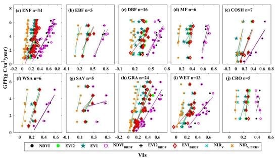
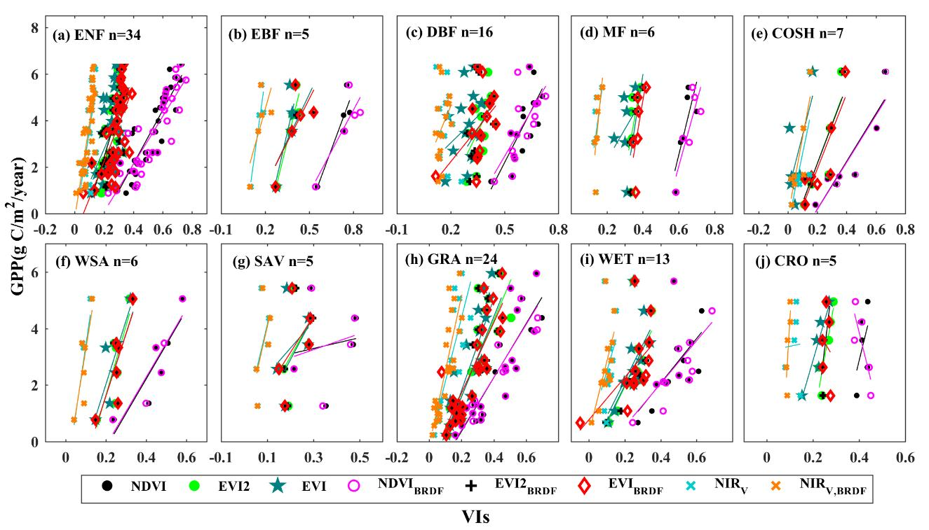
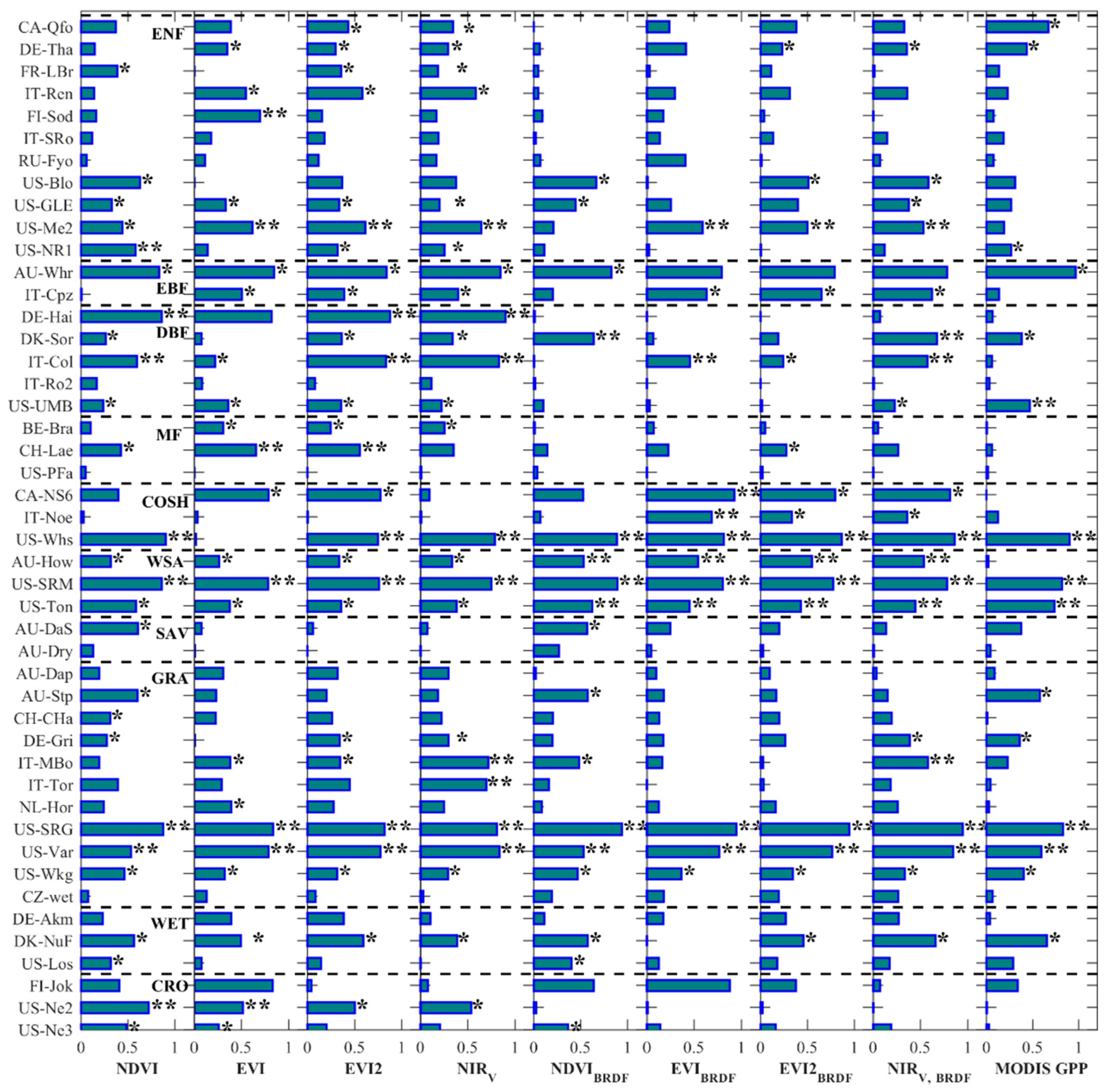
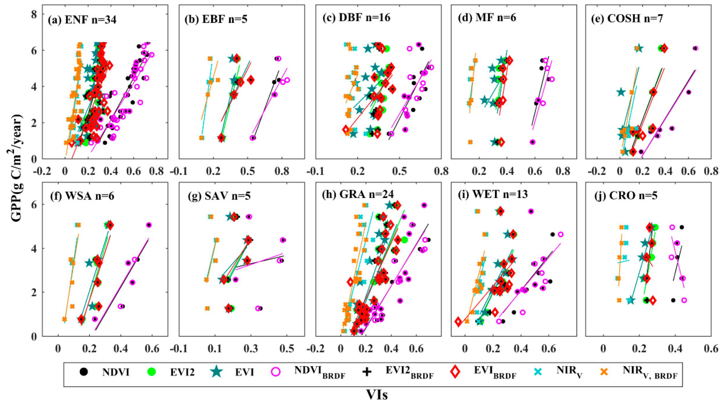
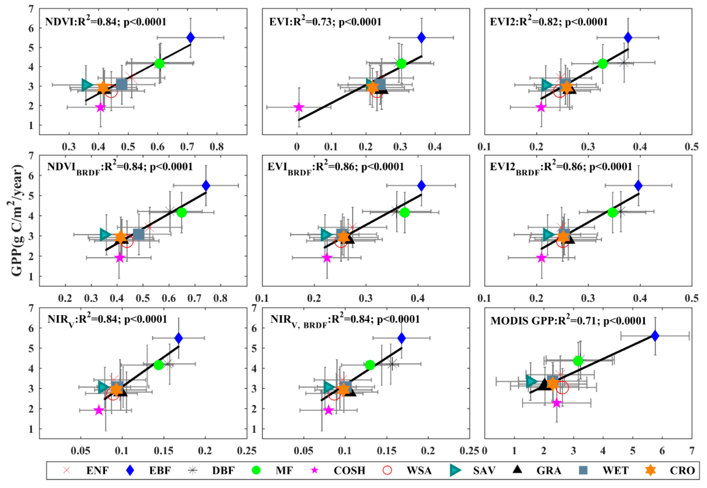
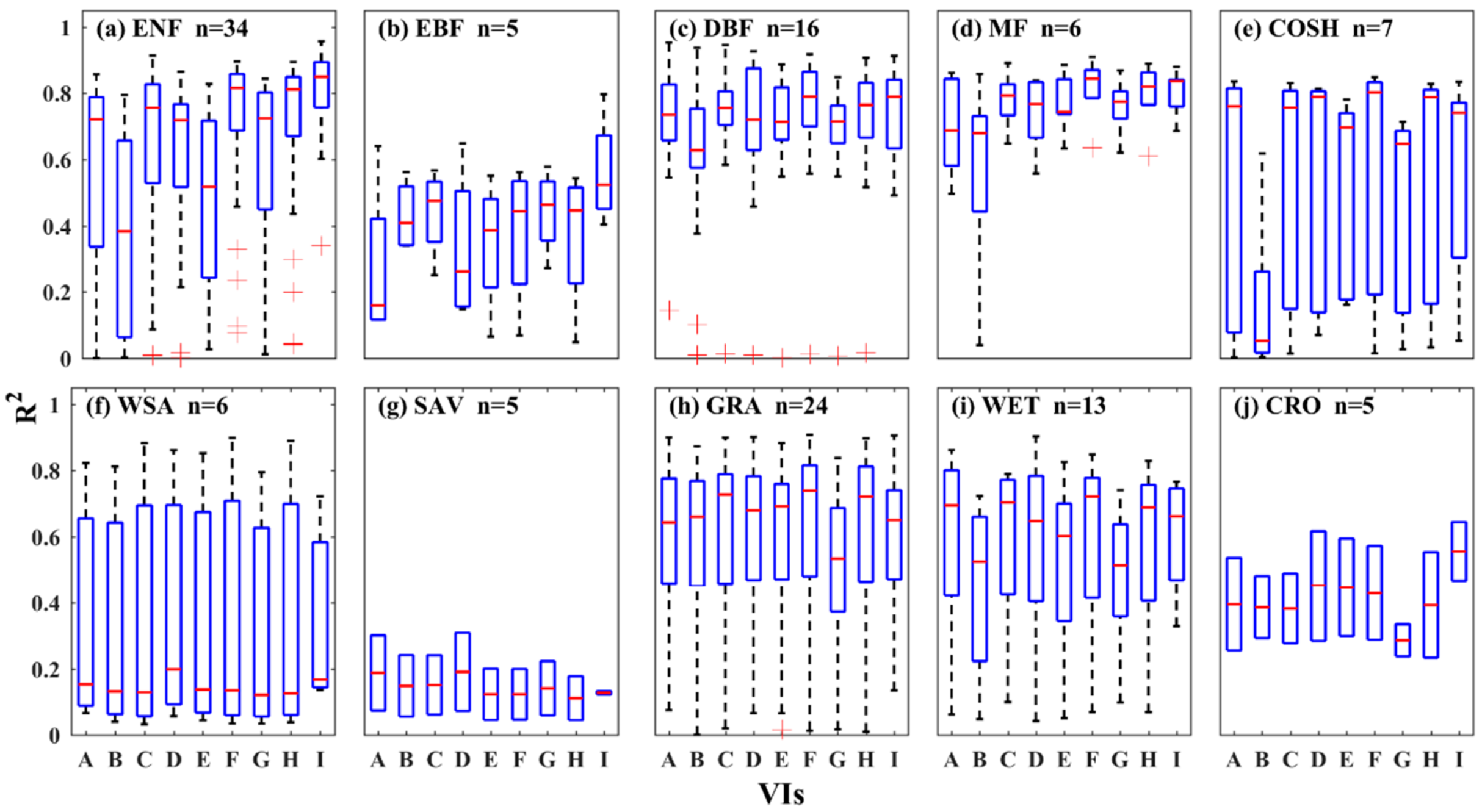
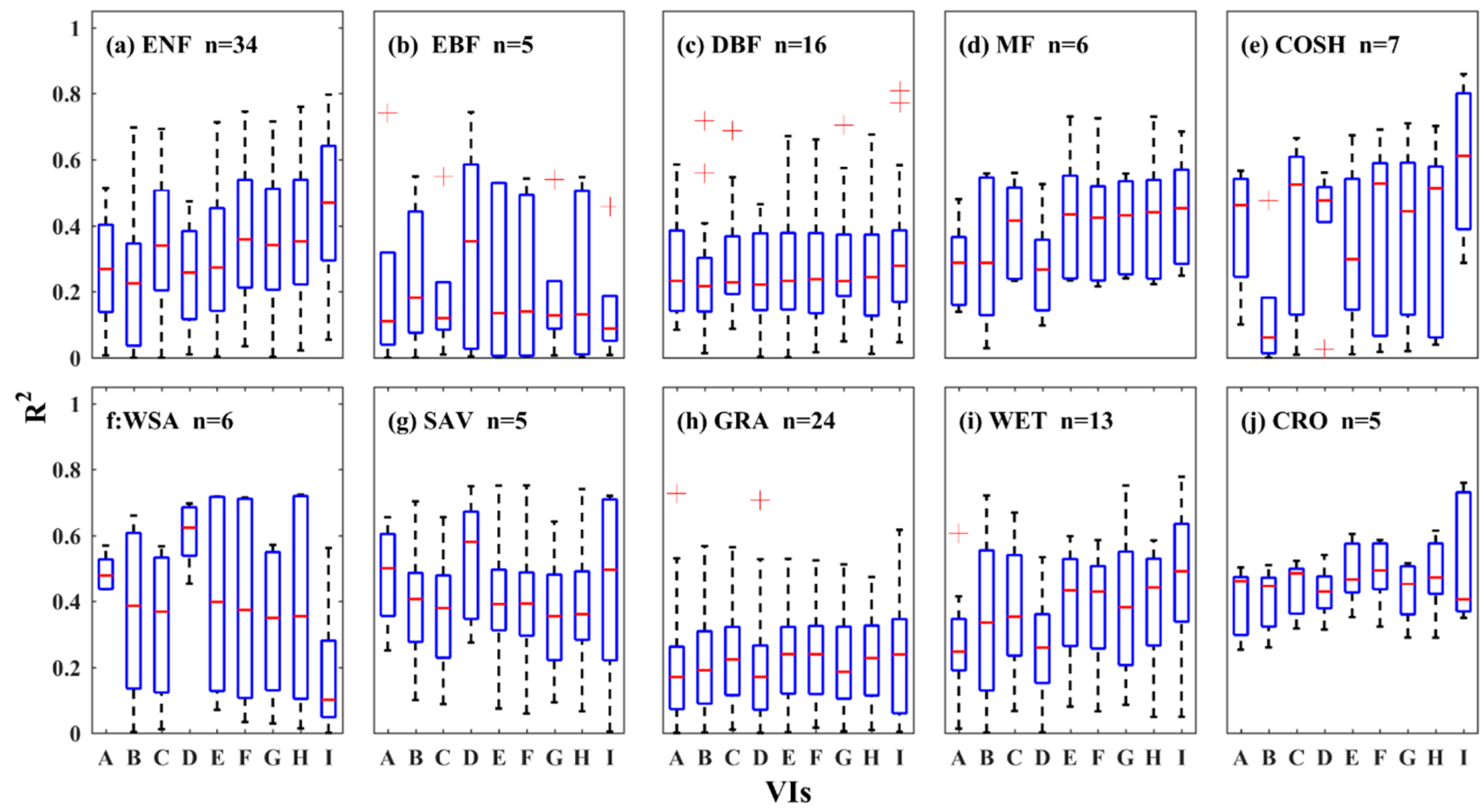
3.1. Relationships between Vegetation Indices and Tower GPP

We examined the relationship between each VI and tower GPP at the monthly scale and calculated the coefficient of determination (R2) for each of the 121 flux sites. For each VI, the R2 values were averaged over the 121 sites. On average, NDVI, EVI, EVI2, NIRV, NDVIBRDF, EVIBRDF, EVI2BRDF, and NIRV, BRDF explained 55%, 48%, 66%, 67%, 56%, 62%, 70%, and 70% of the variance in GPP, respectively. Compared with the traditional VIs (NDVI, EVI, EVI2, and NIRV), the BRDF-corrected VIs (NDVIBRDF, EVIBRDF, EVI2BRDF, and NIRV, BRDF) generally exhibited stronger correlation with tower GPP, indicating that BRDF-corrected VIs had higher performance in estimating GPP than their traditional counterparts at the monthly scale. EVI2BRDF (average R2 = 0.70, p < 0.0001) and NIRV, BRDF (average R2 = 0.70, p < 0.0001) had the strongest correlation with tower GPP. To evaluate the usefulness of the VIs for estimating GPP, we also examined the relationship between MODIS GPP and tower GPP for each flux site. NDVI (55%), EVI (48%), and NDVIBRDF (66%) explained lower variance in tower GPP than did MODIS GPP (70%). By contrast, EVIBRDF, EVI2BRDF, and NIRV, BRDF explained the same proportion (average R2 = 0.70, p < 0.0001) of the variance in tower GPP as did MODIS GPP (Figure 2), although the MODIS GPP is driven by incident photosynthetically active radiation (PAR), the fraction of PAR absorbed by vegetation canopies (fPAR), temperature stress, and water stress. We then stratified the 121 flux sites by biome type. For each biome, the R2 values for the relationship between each VI and tower GPP were averaged over all the sites within the biome. The R2 values for all the ten biomes and VIs are summarized in Figure 2. The performance of each VI generally varied with biome. On average, deciduous broadleaf forests (R2 = 0.65–0.86, p < 0.0001), grasslands (R2 = 0.62–0.72, p < 0.0001), mixed forests (R2 = 0.57–0.86, p < 0.0001), evergreen needleleaf forests (R2 = 0.47–0.82, p < 0.0001) and shrublands (R2 = 0.17–0.77, p < 0.0001) had the strongest correlation, followed by woody savannas (R2 = 0.31–0.61, p < 0.0001), savannas (R2 = 0.35–0.63, p < 0.0001), wetlands (R2 = 0.49–0.68, p < 0.0001) and croplands (R2 = 0.44–0.58, p < 0.0001); evergreen broadleaf forests (R2 = 0.18–0.53, p < 0.0001) had moderate correlation (Table 1).
To examine the relationships between VIs and tower GPP at the annual scale, we identified those sites having at least 6 years of flux data from the 121 FLUXNET sites. A total of 48 sites had at least 6 years of data. For each site, we analyzed the relationships between VIs and tower GPP at the annual scale. For each VI, the R2 values were averaged over all the 48 sites. On average, NDVI, EVI, EVI2, NIRV, NDVIBRDF, EVIBRDF, EVI2BRDF, NIRV, BRDF, and MODIS GPP explained 30%, 29%, 31%, 28%, 25%, 27%, 25%, 30%, and 23% of the variance in tower GPP. This indicates that VIs generally had weaker correlation with tower GPP at the annual scale than at the monthly scale. At the annual scale, the correlation of VIs with tower GPP was comparable to or slightly stronger than MODIS GPP (23%). Compared with the traditional VIs, the BRDF-corrected VIs had no advantage at the annual scale. The relationships between VIs and GPP varied with biome at the annual scale (Figure 3). On average, the relationship was relatively strong for EBF (average R2 = 0.42–0.72), COSH (average R2 = 0.28–0.81), and WSA (average R2 = 0.48–0.68), moderate for ENF (average R2 = 0.16–0.34), GRA (average R2 = 0.29–0.41), WET (average R2 = 0.12–0.34), and CRO (average R2 = 0.09–0.54), and relatively weak for DBF (average R2 = 0.09–0.50) and MF (average R2 = 0.02–0.32). For each biome, the R2 value varied with VI, particularly for ENF, DBF, and COSH.
We then examined the relationships between VIs and tower GPP across all sites for each biome (Figure 4; Table 1). For each site, annual tower GPP and annual mean VIs were separately averaged across all years. Overall, at the site level, tower GPP exhibited moderate to strong relationships with all or most VIs at the annual scale for all biomes except savannas. For savannas, tower GPP was weakly correlated with VIs, particularly NDVI, EVI, and NDVIBRDF. The R2 for the relationship between each VI and GPP varied with biome. There was no universally robust vegetation index that had strong correlation with tower GPP across all ten biomes. Notably, for all biomes except mixed forests, savannas, and croplands, the performance of NDVI, EVI2, EVIBRDF, EVI2BRDF, and NIRV in approximating GPP was comparable to MODIS GPP; for mixed forests, savannas, and croplands, these VIs was more strongly correlated with tower GPP than was MODIS GPP. In addition, at the annual scale, the BRDF-corrected VIs generally had similar performance in approximating GPP as VIs that were not adjusted with BRDF. For example, the traditional NDVI generally performed as well as NDVIBRDF in estimating GPP.
For each biome, the annual VIs and tower GPP averaged across all years were further averaged across all the sites within the biome, and we then examined the relationships between VIs and tower GPP at the biome level (Figure 5). All VIs were strongly correlated with tower GPP across the biomes with R2 ranging from 0.73 to 0.86. The biome averaged EVI had slightly weaker relationship with tower GPP (R2 = 0.73, p < 0.0001) than did other VIs likely due to the low value of EVI in shrublands. Across the ten biomes, EVIBRDF (R2 = 0.86, p < 0.0001) was more strongly correlated with tower GPP than was EVI (R2 = 0.73, p < 0.0001), while NDVIBRDF and EVI2BRDF had comparable performance in estimating GPP to NDVI and EVI2, respectively. All the VIs except EVI were more strongly correlated with averaged tower GPP across the ten biomes than MODIS GPP.

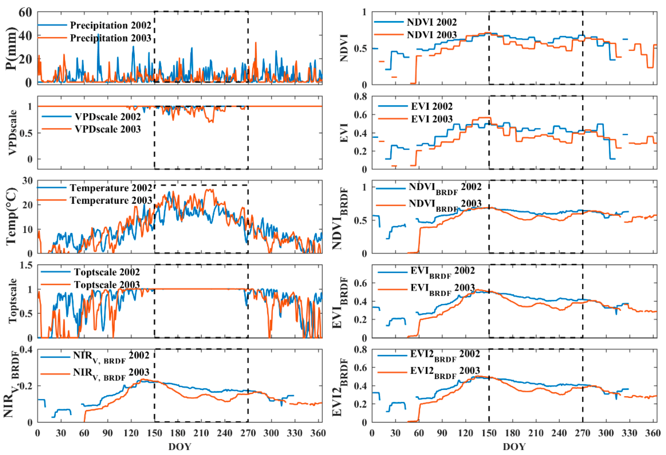
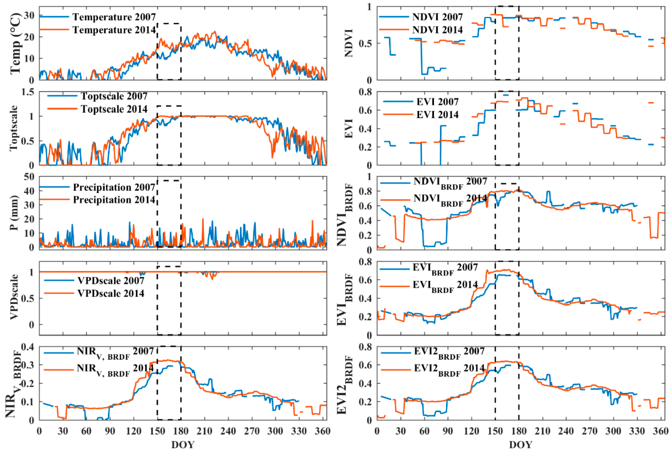
3.2. Relationships between Vegetation Indices and Environmental Stresses

To understand how VIs respond to environmental stresses, we examined the relationships between the VIs and two environmental scalars - fTopt and fVPD (representing temperature stress and water stress, respectively) at the monthly scale for each site separately. On average, NDVI, EVI, EVI2, NIRV, NDVIBRDF, EVIBRDF, EVI2BRDF, and NIRV, BRDF explained 58%, 45%, 61%, 55%, 59%, 53%, 64%, and 62% of the variance in temperature stress across the 121 sites. This indicates that these VIs responded to temperature stress fairly well, and three VIs (EVI2, EVI2BRDF and NIRV, BRDF) could capture temperature stress almost as well as the MODIS GPP product (average R2 = 0.67, p < 0.001). Figure 6 summarizes the R2 values for the relationships between the VIs and the fTopt scalar across all sites in each biome. In general, the correlation of the VIs to temperature stress was high for ENF (R2 = 0.39–0.70, p < 0.0001), DBF (R2 = 0.59–0.73, p < 0.0001), MF (R2 = 0.57–0.81, p < 0.0001), COSH (R2 = 0.16–0.53, p < 0.0001), GRA (R2 = 0.61–0.70, p < 0.0001), and WET (R2 = 0.49–0.64, p < 0.0001), medium for EBF (R2 = 0.27–0.44, p < 0.0001) and CRO (R2 = 0.50–0.60, p < 0.0001), and low for WSA (R2 = 0.06–0.14, p < 0.005) and SAV (R2 = 0.04–0.2, p < 0.5).
NDVI, EVI, EVI2, NIRV, NDVIBRDF, EVIBRDF, EVI2BRDF, and NIRV, BRDF explained 29%, 26%, 32%, 32%, 29%, 31%, 34%, and 34% of the variance in water stress at the monthly scale across 121 sites, respectively. This indicates that these satellite-derived VIs were more strongly correlated with temperature stress than with water stress. Figure 7 summarizes the R2 values for the relationships between the VIs and the water stress scalar across sites for each biome. Compared with the temperature stress scalar (R2 = 0.45–0.64, p < 0.0001), the water stress scalar had weaker correlation with VIs (R2 = 0.26–0.34, p < 0.0001). The correlation of the VIs to water stress was relatively higher for COSH (R2 = 0.13–0.41, p < 0.0001), WSA (R2 = 0.33–0.6, p < 0.0001), SAV (R2 = 0.37–0.52, p < 0.0001), and CRO (R2 = 0.40–0.49, p < 0.0001) and relatively lower for other biomes: ENF (R2 = 0.23–0.38, p < 0.0001), MF (R2 = 0.28–0.44, p < 0.0001) and WET (R2 = 0.25–0.39, p < 0.0001), EBF (R2 = 0.18–0.33, p < 0.0001), DBF (R2 = 0.24–0.29, p < 0.0001) and GRA (R2 = 0.20–0.23, p < 0.0001). For most biomes, VIs generally captured water stress as well as MODIS GPP.
We further chose five sites: DK-Sor (DBF), DE-Hai (DBF), BE-Vie (MF), US-Ne1 (CRO), and CH-Oe1 (GRA) to examine how VIs respond to the low temperature and drought. At CH-Oe1, a grassland site in Switzerland, there was much less precipitation from June to September in 2003 than in 2002, leading to a drought accompanied with high air temperatures during this period in 2003 (Figure 8). During this drought, fVPD decreased with lack of rain while fTopt did not decrease with high temperature; meanwhile, VIs immediately decreased when the drought and high temperature occurred (Figure 8). At US-Ne1, a cropland site in US, there was much less precipitation from June to July in 2003 than in 2004 but relative more rain from August to September in 2003 than in 2004. US-Ne1 and CH-Oe1 exhibited similar responses in fVPD, fTopt, and VIs to drought (Figure S2). At DK-Sor, a DBF site in Denmark, air temperature during the growing season was lower in 2007 than in 2014, and at a result, fTopt and VIs during the growing season were also lower in 2007 than in 2014 (Figure 9). Similarly, at both BE-Vie (a MF site in Germany) (Figure S3) and DE-Hai (a DBF site in Germany), fTopt and VIs during the growing season decreased due to the relatively low temperature (Figure S4).

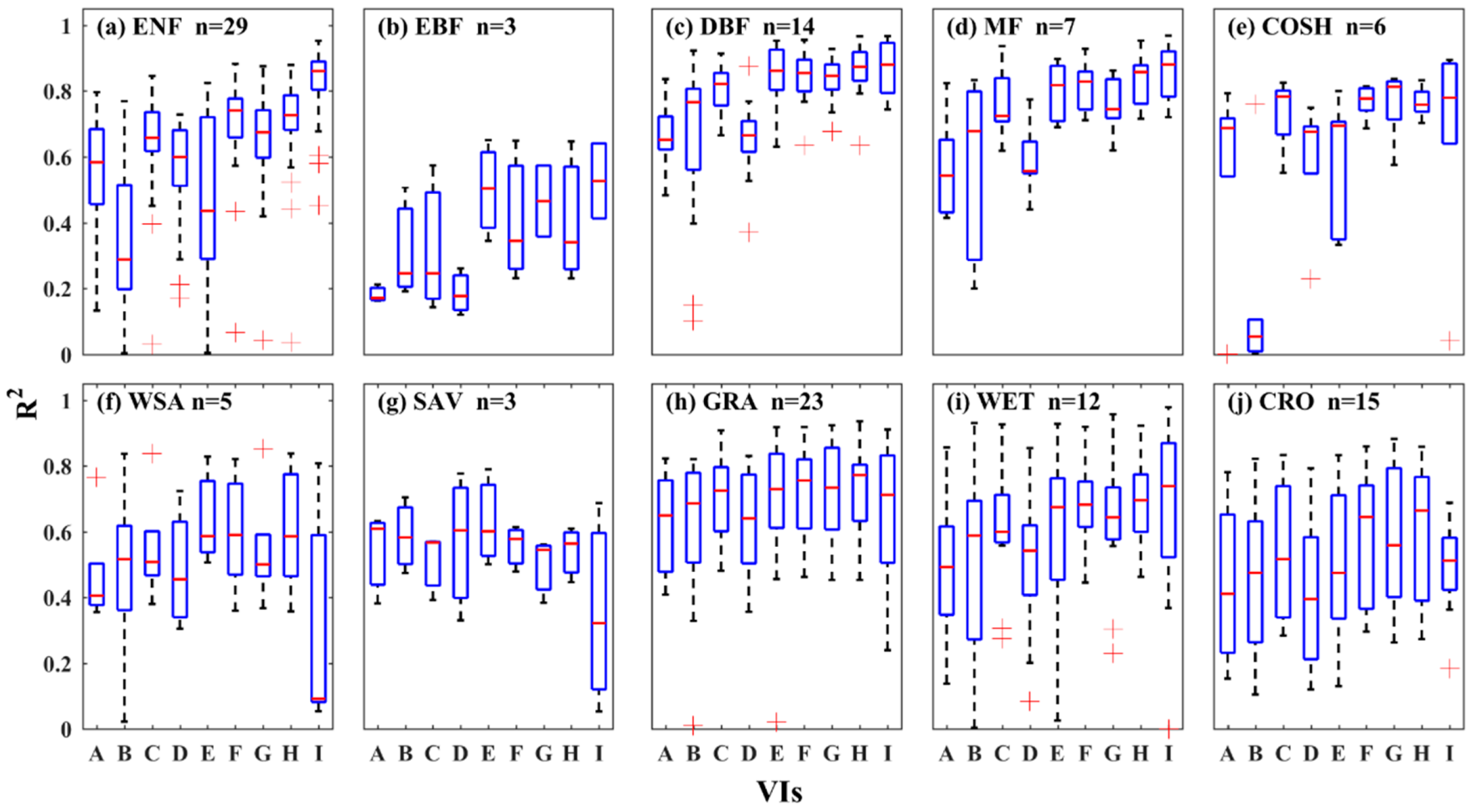
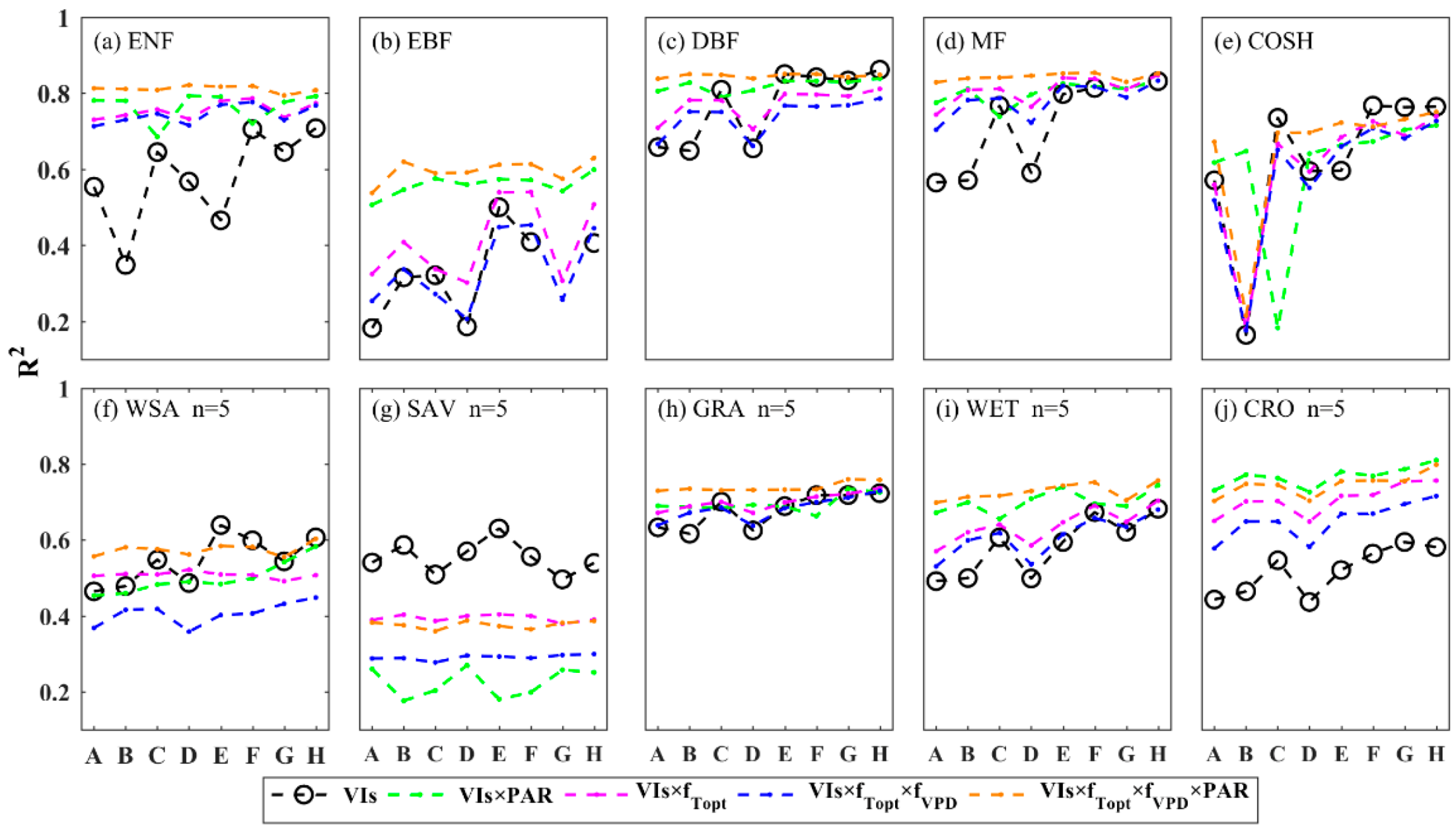
3.3. Relationships between GPP and Vegetation Indices in Combination with Environmental Stresses

To further address how each VI in combination with environmental factors could explain the variations in GPP, we also examined the relationships of GPP with VI × fTopt, VI × fTopt × fVPD and VI × fTopt × fVPD × PAR at the monthly timescale for each site separately. On average, the VIs with temperature stress (VIs × fTopt) explained higher variance in GPP (R2 = 0.64–0.72, p < 0.0001) than VIs with temperature and water stresses (R2 = 0.60–0.70, p < 0.0001) or VIs alone (R2 = 0.48–0.70, p < 0.0001); VIs × fTopt × fVPD × PAR explained the highest variance in GPP (R2 = 0.72–0.76, p < 0.0001) at the monthly timescale for 121 sites. Figure 10 summarizes the R2 values for the relationships between the GPP and the VIs combined with fTopt, fVPD, and PAR in each biome. In general, VIs × fTopt × fVPD × PAR had the strongest relationship with GPP in ten biomes except EBF and SAV where VIs × fTopt × fVPD had the best performance. This indicates that GPP was mainly driven by VIs and also influenced by the environmental stresses and PAR.
The seasonal cycles of the flux tower GPP, two environmental scalars (fTopt and fVPD), and PAR at the NL-Loo site are shown in Figure 11. fTopt exhibited clear seasonal cycles while fVPD was equal to 1.0 most of the time, indicating that temperature limited GPP and VPD was usually not a limiting factor at this site. We chose NIRV, BRDF to examine how VIs combined with environmental scalars and PAR could explain the variance in GPP because NIRV, BRDF had the best performance for predicting GPP (Figure 11). NIRV, BRDF, fTopt, fVPD, and PAR alone explained 73%, 79%, 23%, and 85% of the variance in GPP, respectively. NIRV, BRDF × fTopt (87%) explained the same portion of the variance in GPP as NIRV, BRDF × fTopt × fVPD (86%). Meanwhile, NIRV, BRDF × fTopt × PAR explained the same variance in GPP (R2 = 0.93, p < 0.0001) as NIRV, BRDF × fTopt × fVPD × PAR, indicating that VPD was not a dominant controlling factor of photosynthesis and had negligible contribution at this forest ecosystem (Figure 11).
Similarly, the seasonal cycles of the flux tower GPP, two environmental scalars (fTopt and fVPD), and PAR at the AU-Das site are shown in Figure 12. Unlike NL-Loo, AU-Das exhibited constant values (1.0) for fTopt and clear seasonal cycles for fVPD. At the savanna site, GPP was not affected by fTopt and was weakly influenced by PAR (R2 = 0.03, p < 0.5); NIRV, BRDF × fVPD had a slightly stronger relationship with GPP (R2 = 0.59, p < 0.0001) than NIRV, BRDF (R2 = 0.54, p < 0.0001) or fVPD (R2 = 0.45, p < 0.0001) alone and NIRV, BRDF × fVPD × PAR only explained 3% additional variance in GPP (R2 = 0.62 p < 0.0001) (Figure 12). NIRV, BRDF × PAR (R2 = 0.40, p < 0.0001) had much lower R2 value than NIRV, BRDF × fVPD × PAR (R2 = 0.62 p < 0.0001) (Figure 12). This indicates that temperature was not a limiting factor of GPP but VPD is an important controlling factor at the AU-Das site.

4. Discussion

The concurrent availability of the MODIS record and the FLUXNET2015 database up to 15 years (2000–2014) for a large number of sites across the globe allowed us to examine the relationships between the MODIS-derived VIs and tower GPP at both monthly and annual scales and also to compare these relationships across sites and biomes globally. Our results showed that at the monthly scale there was a strong relationship between each VI and tower GPP for ten biomes except evergreen broadleaf forests. Previous studies also showed close relationships between VIs and GPP. For example, there was a moderate to strong relationship between the daily NDVI and daily GPP for cropland [10], deciduous forest [11], and evergreen forest [12]. Moderate to strong relationships between EVI and GPP at the daily scale were found for grassland [39], temperate evergreen broadleaf forest [40], and wetlands [21]. Previous studies also showed strong correlation between EVI2 and GPP for cropland [10] and evergreen forest [24]. A more recent study showed that the MODIS-derived VIs had strong correlation with tower GPP (R2 = 0.55–0.65, p < 0.0001) at a number of flux sites across eight biomes [2]. The weak relationship for evergreen broadleaf forests found in our study may be caused by the following reasons. First, evergreen broadleaf forests, mainly distributed in the tropics, are more often covered with clouds. Satellite-based indicators are sensitive to cloud contamination or sun-sensor geometry, and the resulting changes in VIs can confound the real seasonality of forests [2]. Second, optical sensors still lack the capability to detect the full canopy activity of the tropical forests. Third, VIs reflect vegetation greenness and are not able to capture seasonal photosynthetic activity of evergreen trees because of the common decoupling of greenness and photosynthesis [41]. Finally, the EC technique can lead to large uncertainty in GPP estimates for these dense, multi-layered forests [42].
Monthly EVI performed slightly better in approximating GPP for seven biomes except ENF, COSH, and SAV than monthly NDVI. Previous studies also found that daily EVI was more useful for estimating GPP in both forest and crop ecosystems than NDVI [43,44]. EVI was more strongly related to GPP than was NDVI likely because EVI does not saturate as rapidly as NDVI when vegetation greenness increases in dense vegetation. Our results showed that EVI2 was a more robust proxy for GPP than was EVI, which supported and substantially expanded the results of the previous studies validating such EVI use for GPP estimation at the daily scale for forest, cropland, and grassland ecosystems [19,44,45]. At short time scales, when the atmospheric effects are insignificant, the blue band does not contribute much additional signal about the land surface than the red band at the canopy level [22]. The two-band EVI2 has no significant loss of information on the land surface, and EVI2 could be even slightly better than the traditional EVI with three bands. Vegetation indices took advantage of NIR band with high reflective properties and red band with absorbed properties of foliage to gain proxies of surface greenness, which were then related to canopy physiology or GPP [23]. Although EVI2 contains the same information as NDVI, the additional weight on the red reflectance in the denominator allows EVI2 to be less sensitive to soil darkening [23], which explained why the EVI2 had the best performance in estimating GPP at the monthly scale among the traditional vegetation indices.
Our results showed that NDVIBRDF, EVIBRDF, EVI2BRDF, and NIRV had stronger relationships with tower GPP than did NDVI, EVI, EVI2, and NIRV, BRDF, respectively, at the month timescale, indicating that the correction of surface reflectance based on BRDF can improve the correlation between VIs and GPP. This finding is consistent with the results of a recent study [2] showing that NDVIBRDF, EVIBRDF, and had stronger relationships with tower GPP than did NDVI and EVI at the daily timescale. Changing illumination and viewing geometry (i.e., Solar Zenith Angle, View Zenith Angle, and Relative Azimuth Angle) can change satellite-measured surface reflectance [28] and the resulting VIs [46]. For example, changes in the sun-sensor geometry could alter EVI across the range of view zenith angles used for most land remote sensing [47]. Another previous study showed that NDVI was highly sensitive to solar zenith angle at intermediate LAI values (0.25–2.00) [48]. It should be noted that for MCD43A4 product, the solar zenith angle is at the local noon, meaning that the solar zenith angle is different at different sites. Moreover, BRDF effects are typically higher in the red wavelength than in the NIR wavelength [46]. Since NDVI captures the difference in reflectance between the NIR and red bands, the BRDF correction could likely alter the behavior of NDVI. Unlike NDVI, with the additional weight on the red band in the denominator, EVI and EVI2 with BRDF correction had varying behaviors because of low BRDF effects in the NIR wavelength and higher BRDF effects in the red wavelength [46]. As a result, the BRDF-corrected VIs performed better in estimating GPP than the traditional VIs without BRDF correction. The different performance of the EVIBRDF and EVI2BRDF resulted from the different formula of the EVI and EVI2. By contrast, the BRDF-corrected VIs had no apparent advantage over the traditional VIs at the annual scale. This is likely because the BRDF effect depends on the sun-object-sensor geometry that changes with season, while the annually averaged sun-object-sensor geometry and BRDF effect do not exhibit interannual variations. Therefore, the correction of BRDF could improve the correlation between BRDF-corrected VIs and tower GPP at the monthly scale but not at the annual scale.
Our results showed that VIs exhibited moderate to strong relationships with tower GPP for EBF, COSH, and WSA and weaker relationships for other biomes at the annual scale. The R2 values for the relationship between the VIs and GPP differed among sites. We examined how the R2 values varied with vegetation cover and water stress. For each site, the Vegetation Continuous Fields (VCF) product [49] derived from MODIS was used to extract the percent vegetation cover (the sum of percent tree cover and percent non-tree cover), and VPD from tower data was used a measure of water stress. The strength of the relationship between VIs and GPP (R2 value) exhibited weak relationships with percent vegetation cover (Table S2) and moderately strong relationships with VPD (Table S3). This indicates that the relationship between VIs and GPP at the annual scale was more dependent on water stress than on vegetation coverage. The performance of the VIs in capturing the interannual variability of tower GPP was generally similar to that of the MODIS GPP product. There is no vegetation index that had strong correlation with tower GPP across all biomes at the annual scale. The correlation between the VIs and tower GPP at the annual scale was generally not as strong as that at the monthly scale for several reasons. First, satellite-derived VIs cannot fully capture the influences of the interannual variability in environmental drivers and biotic factors on GPP [50]. For example, moisture in the root zone, an important ecological factor, can affect annual GPP in crops and seasonally dormant forests, which was not directly observed in the VIs [50]. Second, seasonal changes in the NIR reflectance do not necessarily indicate changes in leaf reflectance, leaf area or vegetation productivity [47]. Third, cloud cover curtails the retrievals of vegetation dynamics and the presence of ephemeral seasonal snow cover can limit the identification of the seasonal change of VIs [51], resulting in the deviation of the VIs at the annual scale. Finally, the interannual variability of GPP was relatively small for some ecosystems such as tropical forests and irrigated croplands [52], and the small ranges in annual VIs and GPP could lead to weaker VI-GPP relationships.
At the site and biome levels, all-around VIs with significant correlation (P < 0.05) to tower GPP only existed in ENF, GRA, WSA, and WET (Table 1) probably due to less seasonal changes of the vegetation canopies in these four ecosystems. NDVI, EVI2, EVIBRDF, EVI2BRDF, and NIRV, BRDF had a relatively better performance in approximating GPP except for SAV and CRO. These results indicate that there is no vegetation index with a strong relationship (R2 >0.7) with tower GPP at the annual scale across all the biomes (Figure 3). At the biome level, the performances of the VIs in predicting GPP were comparable to each other (R2 = 0.84–0.86, p < 0.0001). EVI explained slightly lower variance in GPP (R2 = 0.73, p < 0.0001) probably due to the low values of EVI in open and closed shrublands.
Interestingly, VIs generally had similar performance to the MODIS GPP product in estimating GPP at both monthly and annual timescales. Besides fPAR, three other input variables: PAR, temperature stress, and water stress are explicitly incorporated into the MODIS GPP algorithm. This demonstrates that VIs are generally good proxies of vegetation productivity and can be used to estimate GPP across a wide variety of biomes. Meanwhile, similar to the MODIS GPP product, VIs only explained ~20–30% of the variance in GPP at the annual scale. This indicates that caution should be taken for interpreting the results on the interannual variability and long-term trends in VIs. Capturing the interannual variability and long-term trends in GPP remains a challenge to not only satellite-derived VIs but also light use efficiency and process-based ecosystem models [53,54]. Both observational and modeling studies have reported that the increase of the diffuse radiation improved plant LUE [55,56,57]. The surface reflectance and the resulting VIs do not account for the fraction of diffuse radiation, and therefore the effects of diffuse radiation were not considered.
Our results also showed that these VIs responded to temperature stress fairly well. In particular, three VIs: EVI2, EVI2BRDF, and NIRV, BRDF could capture temperature stress almost as well as the MODIS GPP algorithm that incorporates a temperature scalar. A late spring frost reduced vegetation productivity as approximated by NDVI in a beech dominated Mediterranean mountain forest [58]. Satellite-derived photosynthetic activity approximated by NDVI in the Swiss Alps revealed high-elevation growth enhancement and low-elevation growth suppression in response to the 2003 heat wave [59]. Although VIs were less sensitive to water stress than to temperature stress, VIs generally captured water stress as well as MODIS GPP for most biomes. The VIs respond to dry and wet spells because of their sensitivity to water stress and have been used to examine the responses of vegetation productivity to drought [60,61]. On the other hand, VIs and MODIS GPP explained only a small part of the variance in water stress, indicating that they could not fully capture the effects of water stress on plant productivity.
Our results further indicated that VIs in combination with environmental stresses (temperature stress and water stress) could better explain the variance in GPP. The two environmental stresses - fTopt and fVPD limited GPP during low temperature and drought periods, respectively. For example, VPD is an important controlling factor of GPP at AU-Das (a savanna ecosystem in Australia), while temperature is a dominant controlling factor of the photosynthesis at the NL-Loo site (an ENF ecosystem in Netherlands). Drought can reduce stomatal conductance when hydraulic capacity cannot meet the transpirational demand in a drought season, particularly with increasing atmospheric VPD [62]. Low temperature can inhibit photophysical and photochemical processes involved in light absorption and energy transfer and transformation and can also decrease the rates of the enzymatic reactions including C, N, and S [63,64], leading to the reduction of GPP.

5. Conclusions

Our study made the first comprehensive global analysis of how the traditional vegetation indices (NDVI, EVI, EVI2), BRDF-corrected vegetation indices (NDVIBRDF, EVIBRDF, EVI2BRDF), and a newly proposed vegetation index - NIRV with and without BRDF correction (NIRV, NIRV, BRDF) are related to tower GPP for a total of 121 sites encompassing ten biomes across the globe and at both monthly and annual scales. At the monthly scale, all the eight VIs were moderately or strongly correlated with tower GPP. Compared with the traditional VIs (NDVI, EVI, and EVI2), the BRDF-corrected VIs (NDVIBRDF, EVIBRDF, and EVI2BRDF) generally had stronger correlation with tower GPP, indicating that the VIs based on BRDF-correction had an advantage over the traditional VIs. EVI2BRDF and NIRV, BRDF had the strongest correlation with tower GPP (averaged R2 = 0.70, p < 0.0001), and their performance was comparable to the MODIS GPP product (averaged R2 = 0.70, p < 0.0001) based on a light use model. The VIs explained lower variance in tower GPP at the annual scale than at the monthly scale. BRDF-corrected VIs had no advantage over the traditional counterparts at the annual scale. The capability of the VIs in capturing the interannual variability in GPP was also similar to that of the MODIS GPP product. At the site level, VIs generally exhibited moderate to strong correlation with tower GPP at the annual scale for all biomes except savannas. Similar to the MODIS GPP product, all VIs were strong predictors of GPP at the biome level. Our results also showed that monthly VIs were also influenced by the environmental stresses (temperature stress and water stress). As with the MODIS GPP product, monthly VIs were more sensitive to temperature stress than to water stress. Our findings have implications for improving our understanding of the relationships between satellite-derived VIs and tower GPP, the influences of the BRDF effect on the VI-GPP relationship, and the variations of the VI-GPP relationship among indices, biomes, and timescales.

Supplementary Materials

The following are available online at https://www.mdpi.com/2072-4292/11/15/1823/s1. Figure S1: Flux tower GPP (GPPEC) and MODIS-derived VIs against latitude: (a) GPP; (b) VIs. There are no significant relationships between VIs (GPP) and latitude. Figure S2: Daily VIs, temperature, precipitation, temperature stress (fTopt) and water stress (fVPD) in croplands site (US-Ne1) in a normal period from August to September in 2003 and a drought period from June to July in 2004. Figure S3: VIs, temperature, precipitation, temperature stress (fTopt) and water stress (fVPD) at mixed forest site (BE-Vie) in a normal year (2010) and a low temperature year (2011). Figure S4: Daily VIs, temperature, precipitation, temperature stress (fTopt) and water stress (fVPD) in deciduous broadleaf forest site (DE-Hai) in a normal year (2003) and a relative low temperature year (2004). Table S1: List of 121 eddy covariance flux tower sites used in this study. IGBP refers to the International Geosphere-Biosphere Program land cover classification. ENF: evergreen needleleaf forest; EBF: evergreen broadleaf forest; DBF: deciduous broadleaf forest; MF: mixed forest; OCSH: open and closed shrublands; SAV: savannas; WSA: woody savannas; GRA: grassland; CRO: cropland; WET: wetland. Table S2: The correlation of R2 of the relationships between VIs and tower-based GPP with vegetation coverage at the annual scale across all sites. The asterisks - *, ** and *** stand for the significance level p < 0.05, p < 0.01 and p < 0.001, respectively. Table S3: The correlation of R2 of of the relationships between VIs and tower-based GPP with VPD at the annual scale across all sites. The asterisks - *, ** and *** stand for the significance level p < 0.05, p < 0.01 and p < 0.001, respectively.

Author Contributions

Conceptualization, J.X. and X.H.; Methodology, X.H., J.X. and M.M.; Formal Analysis, X.H. and J.X.; Writing—Original Draft Preparation, X.H.; Writing—Review & Editing, J.X. and M.M.; Supervision, J.X.; Funding Acquisition, J.X. and M.M.

Funding

This study was supported by both China’s funding agencies (the National Natural Science Foundation of China: Grant No. 41830648 & 41771453; National Key Technology R&D Program of China: Grant No. 2016YFC0500106) and U.S. funding agencies (National Aeronautics and Space Administration (NASA) through the Carbon Cycle Science Program: Grant No. NNX14AJ18G and the Climate Indicators and Data Products for Future National Climate Assessments: Grant No. NNX16AG61G).

Acknowledgments

We thank the PIs of the FLUXNET Tier-1 sites and MODIS products (surface reflectance and GPP) for making the datasets available to the research community. This work used eddy covariance data acquired and shared by the FLUXNET community, including these networks: AmeriFlux, AfriFlux, AsiaFlux, CarboAfrica, CarboEuropeIP, CarboItaly, CarboMont, ChinaFlux, Fluxnet-Canada, GreenGrass, ICOS, KoFlux, LBA, NECC, OzFlux-TERN, TCOS-Siberia, and USCCC. The ERA-Interim reanalysis data are provided by ECMWF and processed by LSCE. The FLUXNET eddy covariance data processing and harmonization was carried out by the European Fluxes Database Cluster, AmeriFlux Management Project, and Fluxdata project of FLUXNET, with the support of CDIAC and ICOS Ecosystem Thematic Center, and the OzFlux, ChinaFlux and AsiaFlux offices. All the MODIS data products can be downloaded from the Oak Ridge National Laboratory (ORNL)’s Distributed Active Archive Center (DAAC) (https://modis.ornl.gov/cgi-bin/MODIS/global/subset.pl). All the flux and meteorological data are available from the FLUXNET2015 Dataset website (http://fluxnet.fluxdata.org/data/fluxnet2015-dataset/). We thank the two anonymous reviewers for their constructive and insightful comments on our manuscript.

Conflicts of Interest

The authors declare no conflict of interest.

References

  1. Li, X.; Xiao, J.; He, B. Chlorophyll fluorescence observed by OCO-2 is strongly related to gross primary productivity estimated from flux towers in temperate forests. Remote Sens. Environ. 2018, 204, 659–671. [Google Scholar] [CrossRef]
  2. Li, X.; Xiao, J.; He, B.; Altaf Arain, M.; Beringer, J.; Desai, A.R.; Emmel, C.; Hollinger, D.Y.; Krasnova, A.; Mammarella, I.; et al. Solar-induced chlorophyll fluorescence is strongly correlated with terrestrial photosynthesis for a wide variety of biomes: First global analysis based on OCO-2 and flux tower observations. Glob. Chang. Biol. 2018. [Google Scholar] [CrossRef] [PubMed]
  3. Xiao, J.F.; Moody, A. A comparison of methods for estimating fractional green vegetation cover within a desert-to-upland transition zone in central New Mexico, USA. Remote Sens. Environ. 2005, 98, 237–250. [Google Scholar] [CrossRef]
  4. Zhou, L.; Tian, Y.; Myneni, R.B.; Ciais, P.; Saatchi, S.; Liu, Y.Y.; Piao, S.; Chen, H.; Vermote, E.F.; Song, C.; et al. Widespread decline of Congo rainforest greenness in the past decade. Nature 2014, 509, 86–90. [Google Scholar] [CrossRef] [PubMed]
  5. Nagai, S.; Saigusa, N.; Muraoka, H.; Nasahara, K.N. What makes the satellite-based EVI-GPP relationship unclear in a deciduous broad-leaved forest? Ecol. Res. 2010, 25, 359–365. [Google Scholar] [CrossRef]
  6. Shi, H.; Li, L.H.; Eamus, D.; Huete, A.; Cleverly, J.; Tian, X.; Yu, Q.; Wang, S.Q.; Montagnani, L.; Magliulo, V.; et al. Assessing the ability of MODIS EVI to estimate terrestrial ecosystem gross primary production of multiple land cover types. Ecol. Indic. 2017, 72, 153–164. [Google Scholar] [CrossRef] [Green Version]
  7. Sims, D.A.; Rahman, A.F.; Cordova, V.D.; El-Masri, B.Z.; Baldocchi, D.D.; Flanagan, L.B.; Goldstein, A.H.; Hollinger, D.Y.; Misson, L.; Monson, R.K.; et al. On the use of MODIS EVI to assess gross primary productivity of North American ecosystems. J. Geophys. Res. 2006. [Google Scholar] [CrossRef]
  8. Xiao, J.F.; Zhou, Y.; Zhang, L. Contributions of natural and human factors to increases in vegetation productivity in China. Ecosphere 2015, 6, 233. [Google Scholar] [CrossRef]
  9. Rouse, J.W. Monitoring the Vernal Advancement and Retrogradation (Green Wave Effect) of Natural Vegetation; NASA Gsfct Type Report; Texas A&M University: College Station, TX, USA, 1973; p. 120. [Google Scholar]
  10. Peng, Y.; Gitelson, A.A. Remote estimation of gross primary productivity in soybean and maize based on total crop chlorophyll content. Remote Sens. Environ. 2012, 117, 440–448. [Google Scholar] [CrossRef]
  11. Birky, A.K. NDVI and a simple model of deciduous forest seasonal dynamics. Ecol. Model. 2001, 143, 43–58. [Google Scholar] [CrossRef]
  12. Wang, Q.; Tenhunen, J.; Dinh, N.Q.; Reichstein, M.; Vesala, T.; Keronen, P. Similarities in ground- and satellite-based NDVI time series and their relationship to physiological activity of a Scots pine forest in Finland. Remote Sens. Environ. 2004, 93, 30. [Google Scholar] [CrossRef]
  13. Huete, A.R.; Jackson, R.D.; Post, D.F. Spectral Response of a Plant Canopy with Different Soil Backgrounds. Remote Sens. Environ. 1985, 17, 37–53. [Google Scholar] [CrossRef]
  14. Ben-Ze’ev, E.; Karnieli, A.; Agam, N.; Kaufman, Y.; Holben, B. Assessing vegetation condition in the presence of biomass burning smoke by applying the Aerosol-free Vegetation Index (AFRI) on MODIS images. Int. J. Remote Sens. 2006, 27, 3203–3221. [Google Scholar] [CrossRef]
  15. Carlson, T.N.; Ripley, D.A. On the relation between NDVI, fractional vegetation cover, and leaf area index. Remote Sens. Environ. 1997, 62, 241–252. [Google Scholar] [CrossRef]
  16. Gitelson, A.A. Wide Dynamic Range Vegetation Index for Remote Quantification of Biophysical Characteristics of Vegetation. J. Plant Physiol. 2004, 161, 165–173. [Google Scholar] [CrossRef] [Green Version]
  17. Huete, A.; Didan, K.; Miura, T.; Rodriguez, E.P.; Gao, X.; Ferreira, L.G. Overview of the radiometric and biophysical performance of the MODIS vegetation indices. Remote Sens. Environ. 2002, 83, 195–213. [Google Scholar] [CrossRef]
  18. Huete, A.R.; Liu, H.Q.; Batchily, K.; Van Leeuwen, W. A comparison of vegetation indices over a global set of TM images for EOS-MODIS. Remote Sens. Environ. 1997, 59, 440–451. [Google Scholar] [CrossRef]
  19. Li, Z.; Yu, G.; Xiao, X.; Li, Y.; Zhao, X.; Ren, C.; Zhang, L.; Fu, Y. Modeling gross primary production of alpine ecosystems in the Tibetan Plateau using MODIS images and climate data. Remote Sens. Environ. 2007, 107, 510–519. [Google Scholar] [CrossRef]
  20. Wu, C.Y.; Munger, J.W.; Niu, Z.; Kuang, D. Comparison of multiple models for estimating gross primary production using MODIS and eddy covariance data in Harvard Forest. Remote Sens. Environ. 2010, 114, 2925–2939. [Google Scholar] [CrossRef]
  21. Gao, Y.; Ouyang, Z.; Shao, C.; Chu, H.; Su, Y.J.; Guo, H.; Chen, J.; Zhao, B. Field Observation of Lateral Detritus Carbon Flux in a Coastal Wetland. Wetlands 2018, 38, 613–625. [Google Scholar] [CrossRef]
  22. Jiang, Z.Y.; Huete, A.R.; Didan, K.; Miura, T. Development of a two-band enhanced vegetation index without a blue band. Remote Sens. Environ. 2008, 112, 3833–3845. [Google Scholar] [CrossRef]
  23. Rocha, A.V.; Shaver, G.R. Advantages of a two band EVI calculated from solar and photosynthetically active radiation fluxes. Agric. For. Meteorol. 2009, 149, 1560–1563. [Google Scholar] [CrossRef]
  24. Gusso, A.; Lee, J.; Son, Y.; Son, Y.M. Empirical Relationship between Leaf Biomass of Red Pine Forests and Enhanced Vegetation Index in South Korea Using Landsat-5 Tm. ISPRS Ann. Photogramm. Remote Sens. Spat. Inf. Sci. 2016, 3, 79–83. [Google Scholar] [CrossRef]
  25. Huete, A.R.; Miura, T.; Kim, Y.; Didan, K.; Privette, J. Assessments of multisensor vegetation index dependencies with hyperspectral and tower flux data. Remote Sens. Model. Ecosyst. Sustain. III 2006. [Google Scholar] [CrossRef]
  26. Xiao, X.; Hollinger, D.; Aber, J.; Goltz, M.; Davidson, E.A.; Zhang, Q.; Moore, B. Satellite-based modeling of gross primary production in an evergreen needleleaf forest. Remote Sens. Environ. 2004, 89, 519–534. [Google Scholar] [CrossRef]
  27. Zhou, L.; Tucker, C.J.; Kaufmann, R.K.; Slayback, D.; Shabanov, N.V.; Myneni, R.B. Variations in northern vegetation activity inferred from satellite data of vegetation index during 1981 to 1999. J. Geophys. Res. Atmos. 2001, 106, 20069–20084. [Google Scholar] [CrossRef]
  28. Schaaf, C.B.; Gao, F.; Strahler, A.H.; Lucht, W.; Li, X.; Tsang, T.; Strugnell, N.C.; Zhang, X.; Jin, Y.; Muller, J.P.; et al. First operational BRDF, albedo nadir reflectance products from MODIS. Remote Sens. Environ. 2002, 83, 135–148. [Google Scholar] [CrossRef] [Green Version]
  29. Lucht, W.; Schaaf, C.B.; Strahler, A.H. An algorithm for the retrieval of albedo from space using semiempirical BRDF models. IEEE Trans. Geosci. Remote Sens. 2000, 38, 977–998. [Google Scholar] [CrossRef] [Green Version]
  30. Xiao, J. Satellite evidence for significant biophysical consequences of the “Grain for Green” program on the loess plateau in China. J. Geophys. Res. Biogeosci. 2014, 119, 2261–2275. [Google Scholar] [CrossRef]
  31. Sjöström, M.; Ardö, J.; Arneth, A.; Boulain, N.; Cappelaere, B.; Eklundh, L.; de Grandcourt, A.; Kutsch, W.L.; Merbold, L.; Nouvellon, Y.; et al. Exploring the potential of MODIS EVI for modeling gross primary production across African ecosystems. Remote Sens. Environ. 2011, 115, 1081–1089. [Google Scholar] [CrossRef]
  32. Badgley, G.; Field, C.B.; Berry, J.A. Canopy near-infrared reflectance and terrestrial photosynthesis. Sci. Adv. 2017, 3, e1602244. [Google Scholar] [CrossRef]
  33. Reichstein, M.; Falge, E.; Baldocchi, D.; Papale, D.; Aubinet, M.; Berbigier, P.; Bernhofer, C.; Buchmann, N.; Gilmanov, T.; Granier, A.; et al. On the separation of net ecosystem exchange into assimilation and ecosystem respiration: Review and improved algorithm. Glob. Chang. Biol. 2005, 11, 1424–1439. [Google Scholar] [CrossRef]
  34. Lasslop, G.; Reichstein, M.; Papale, D.; Richardson, A.D.; Arneth, A.; Barr, A.; Stoy, P.; Wohlfahrt, G. Separation of net ecosystem exchange into assimilation and respiration using a light response curve approach: Critical issues and global evaluation. Glob. Chang. Biol. 2010, 16, 187–208. [Google Scholar] [CrossRef]
  35. Rahman, A.F.; Sims, D.A.; Cordova, V.D.; El-Masri, B.Z. Potential of MODIS EVI and surface temperature for directly estimating per-pixel ecosystem C fluxes. Geophys. Res. Lett. 2005. [Google Scholar] [CrossRef]
  36. Waring, R.H.; Coops, N.C.; Fan, W.; Nightingale, J.M. MODIS enhanced vegetation index predicts tree species richness across forested ecoregions in the contiguous USA. Remote Sens. Environ. 2006, 103, 218–226. [Google Scholar] [CrossRef]
  37. Karnieli, A.; Kaufman, Y.J.; Remer, L.; Wald, A. AFRI—Aerosol free vegetation index. Remote Sens. Environ. 2001, 77, 10–21. [Google Scholar] [CrossRef]
  38. Zhao, M.S.; Heinsch, F.A.; Nemani, R.R.; Running, S.W. Improvements of the MODIS terrestrial gross and net primary production global data set. Remote Sens. Environ. 2005, 95, 164–176. [Google Scholar] [CrossRef]
  39. Liu, J.F.; Chen, S.P.; Han, X.G. Modeling gross primary production of two steppes in Northern China using MODIS time series and climate data. Procedia Environ. Sci. 2012, 13, 742–754. [Google Scholar] [CrossRef] [Green Version]
  40. Renchon, A.A.; Griebel, A.; Metzen, D.; Williams, C.A.; Medlyn, B.; Duursma, R.A.; Barton, C.V.M.; Maier, C.; Boer, M.M.; Isaac, P.; et al. Upside-down fluxes Down Under: CO2 net sink in winter and net source in summer in a temperate evergreen broadleaf forest. Biogeosciences 2018, 15, 3703–3716. [Google Scholar] [CrossRef] [Green Version]
  41. Smith, W.K.; Biederman, J.A.; Scott, R.L.; Moore, D.J.P.; He, M.; Kimball, J.S.; Yan, D.; Hudson, A.; Barnes, M.L.; MacBean, N.; et al. Chlorophyll Fluorescence Better Captures Seasonal and Interannual Gross Primary Productivity Dynamics Across Dryland Ecosystems of Southwestern North America. Geophys. Res. Lett. 2018, 45, 748–757. [Google Scholar] [CrossRef]
  42. Hayek, M.N.; Wehr, R.; Longo, M.; Hutyra, L.R.; Wiedemann, K.; Munger, J.W.; Bonal, D.; Saleska, S.R.; Fitzjarrald, D.R.; Wofsy, S.C. A novel correction for biases in forest eddy covariance carbon balance. Agric. For. Meteorol. 2018, 250, 90–101. [Google Scholar] [CrossRef]
  43. Sims, D.; Rahman, A.; Cordova, V.; Elmasri, B.; Baldocchi, D.; Bolstad, P.; Flanagan, L.; Goldstein, A.; Hollinger, D.; Misson, L. A new model of gross primary productivity for North American ecosystems based solely on the enhanced vegetation index and land surface temperature from MODIS. Remote Sens. Environ. 2008, 112, 1633–1646. [Google Scholar] [CrossRef]
  44. Wu, C.Y.; Han, X.Z.; Ni, J.S.; Niu, Z.; Huang, W.J. Estimation of gross primary production in wheat from in situ measurements. Int. J. Appl. Earth Obs. Geoinf. 2010, 12, 183–189. [Google Scholar] [CrossRef]
  45. Peng, Y.; Gitelson, A.A.; Keydan, G.; Rundquist, D.C.; Moses, W. Remote estimation of gross primary production in maize and support for a new paradigm based on total crop chlorophyll content. Remote Sens. Environ. 2011, 115, 978–989. [Google Scholar] [CrossRef]
  46. Buchhorn, M.; Raynolds, M.K.; Walker, D.A. Influence of BRDF on NDVI and biomass estimations of Alaska Arctic tundra. Environ. Res. Lett. 2016, 11, 125002. [Google Scholar] [CrossRef]
  47. Morton, D.C.; Nagol, J.; Carabajal, C.C.; Rosette, J.; Palace, M.; Cook, B.D.; Vermote, E.F.; Harding, D.J.; North, P.R.J. Amazon forests maintain consistent canopy structure and greenness during the dry season. Nature 2014, 506, 221–224. [Google Scholar] [CrossRef]
  48. Goward, S.N.; Huemmrich, K.F. Vegetation Canopy Par Absorptance and the Normalized Difference Vegetation Index—An Assessment Using the Sail Model. Remote Sens. Environ. 1992, 39, 119–140. [Google Scholar] [CrossRef]
  49. DiMiceli, C.; Carroll, M.; Sohlberg, R.; Huang, M.C.; Hansen, M.; Townsend, J.R.G. Annual Global Automated MODIS Vegetation Continuous Fields (MOD44B) at 250 m Spatial Resolution for Data Years Beginning Day 65, 2000–2010, Collection 5, Version 1; University of Maryland: College Park, MD, USA, 2011. [Google Scholar]
  50. Verma, M.; Friedl, M.A.; Richardson, A.D.; Kiely, G.; Cescatti, A.; Law, B.E.; Wohlfahrt, G.; Gielen, B.; Roupsard, O.; Moors, E.J.; et al. Remote sensing of annual terrestrial gross primary productivity from MODIS: An assessment using the FLUXNET La Thuile data set. Biogeosciences 2014, 11, 2185–2200. [Google Scholar] [CrossRef]
  51. Zhang, X. Reconstruction of a complete global time series of daily vegetation index trajectory from long-term AVHRR data. Remote Sens. Environ. 2015, 156, 457–472. [Google Scholar] [CrossRef]
  52. Xiao, J.F.; Liu, S.G.; Stoy, P.C. Preface: Impacts of extreme climate events and disturbances on carbon dynamics. Biogeosciences 2016, 13, 3665–3675. [Google Scholar] [CrossRef] [Green Version]
  53. Huntzinger, D.N.; Post, W.M.; Wei, Y.; Michalak, A.M.; West, T.O.; Jacobson, A.R.; Baker, I.T.; Chen, J.M.; Davis, K.J.; Hayes, D.J.; et al. North American Carbon Program (NACP) regional interim synthesis: Terrestrial biospheric model intercomparison. Ecol. Model. 2012, 232, 144–157. [Google Scholar] [CrossRef] [Green Version]
  54. Thorn, A.M.; Xiao, J.; Ollinger, S.V. Generalization and evaluation of the process-based forest ecosystem model PnET-CN for other biomes. Ecosphere 2015, 6, 1–27. [Google Scholar] [CrossRef]
  55. Gu, L.; Baldocchi, D.; Verma, S.B.; Black, T.A.; Vesala, T.; Falge, E.M.; Dowty, P.R. Advantages of diffuse radiation for terrestrial ecosystem productivity. J. Geophys. Res. Atmos. 2002, 107, ACL 2-1–ACL 2-23. [Google Scholar] [CrossRef]
  56. Dengel, S.; Grace, J. Carbon dioxide exchange and canopy conductance of two coniferous forests under various sky conditions. Oecologia 2010, 164, 797–808. [Google Scholar] [CrossRef]
  57. Oliphant, A.J.; Dragoni, D.; Deng, B.; Grimmond, C.S.B.; Schmid, H.P.; Scott, S.L. The role of sky conditions on gross primary production in a mixed deciduous forest. Agric. For. Meteorol. 2011, 151, 781–791. [Google Scholar] [CrossRef]
  58. Nolè, A.; Rita, A.; Ferrara, A.M.S.; Borghetti, M. Effects of a large-scale late spring frost on a beech (Fagus sylvatica L.) dominated Mediterranean mountain forest derived from the spatio-temporal variations of NDVI. Ann. For. Sci. 2018, 75, 83. [Google Scholar] [CrossRef]
  59. Jolly, W.M.; Dobbertin, M.; Zimmermann, N.E.; Reichstein, M. Divergent vegetation growth responses to the 2003 heat wave in the Swiss Alps. Geophys. Res. Lett. 2005, 32, L18409. [Google Scholar] [CrossRef]
  60. Klisch, A.; Atzberger, C. Operational Drought Monitoring in Kenya Using MODIS NDVI Time Series. Remote Sens. 2016, 8, 267. [Google Scholar] [CrossRef]
  61. Zhang, L.; Xiao, J.F.; Li, J.; Wang, K.; Lei, L.P.; Guo, H.D. The 2010 spring drought reduced primary productivity in southwestern China. Environ. Res. Lett. 2012, 7, 045706. [Google Scholar] [CrossRef] [Green Version]
  62. Lee, J.-E.; Frankenberg, C.; Van Der Tol, C.; Berry, J.A.; Guanter, L.; Boyce, C.K. Forest productivity and water stress in Amazonia: Observations from GOSAT chlorophyll fluorescence. Proc. Biol. Sci. 2013, 280, 20130171. [Google Scholar] [CrossRef]
  63. Ensminger, I.; Busch, F.; Huner, N.P.A. Photostasis and cold acclimation: sensing low temperature through photosynthesis. Physiol. Plant. 2006, 126, 28–44. [Google Scholar] [CrossRef]
  64. Huner, N.P.A.; Öquist, G.; Sarhan, F. Energy balance and acclimation to light and cold. Trends Plant Sci. 1998, 3, 224–230. [Google Scholar] [CrossRef]
Figure 1. Location and distribution of the 121 eddy covariance (EC) flux sites used in our study. The site description of these FLUXNET sites is provided in Table S1 in the Supplementary Material. The base map is the MODIS land cover map.
Remotesensing 11 01823 g001
Figure 2. The boxplots of the R2 values for the relationships between MODIS-derived VIs and tower GPP at the monthly scale across all sites within each biome. The letters on the x axis stand for: A - NDVI, B - EVI, C - EVI2, D - NDVIBRDF, E - EVIBRDF, F - EVI2BRDF, G - NIRV, H - NIRV, BRDF, and I - MODIS GPP. The biome types are as follows: evergreen needleleaf forest (ENF); evergreen broadleaf forest (EBF); deciduous needleleaf forest (DNF); mixed forest (MF); closed and open shrublands (COSH); woody savannas (WSA); savannas (SAV); grasslands (GRA); wetlands (WET); croplands (CRO).
Remotesensing 11 01823 g002
Figure 3. The bar graphs of the R2 values for the relationships between the annual averaged VIs and tower GPP for all the sites with at least six years of flux data for each biome. The letters on the x axis stand for the R2 values; the letters on the y axis stand for the sites. The asterisks - * and ** stand for the significance level p < 0.1 and p < 0.05, respectively. The biome types are as follows: evergreen needleleaf forest (ENF); evergreen broadleaf forest (EBF); deciduous needleleaf forest (DNF); mixed forest (MF); closed and open shrublands (COSH); woody savannas (WSA); savannas (SAV); grasslands (GRA); wetlands (WET); croplands (CRO).
Remotesensing 11 01823 g003
Figure 4. The relationships between VIs and tower GPP across all sites for each biome. The R2 values for the relationships between VIs and tower GPP at each biome were provided in Table 1. The biome types are as follows: evergreen needleleaf forest (ENF); evergreen broadleaf forest (EBF); deciduous needleleaf forest (DNF); mixed forest (MF); closed and open shrublands (COSH); woody savannas (WSA); savannas (SAV); grasslands (GRA); wetlands (WET); croplands (CRO).
Remotesensing 11 01823 g004
Figure 5. The relationships of VIs and MODIS GPP with tower GPP across ten biomes. The error bars are standard deviations across all sites within each biome. The biome types are as follows: evergreen needleleaf forest (ENF); evergreen broadleaf forest (EBF); deciduous needleleaf forest (DNF); mixed forest (MF); closed and open shrublands (COSH); woody savannas (WSA); savannas (SAV); grasslands (GRA); wetlands (WET); croplands (CRO).
Remotesensing 11 01823 g005
Figure 6. The boxplots of the R2 values for the relationships of monthly averaged VIs and MODIS GPP with temperature stress (fTopt) for each biome with the total of 121 sites. The letters on the x axis stand for: A - NDVI, B - EVI, C - EVI2, D - NDVIBRDF, E - EVIBRDF, F - EVI2BRDF, G - NIRV, H - NIRV, BRDF, and I - MODIS GPP. The biome types are as follows: evergreen needleleaf forest (ENF); evergreen broadleaf forest (EBF); deciduous needleleaf forest (DNF); mixed forest (MF); closed and open shrublands (COSH); woody savannas (WSA); savannas (SAV); grasslands (GRA); wetlands (WET); croplands (CRO).
Remotesensing 11 01823 g006
Figure 7. The boxplots of the R2 for the relationships of monthly averaged VIs and MODIS GPP with water stress (fVPD) for each biome with the total of 121 sites. The letters on the x axis stand for: A - NDVI, B - EVI, C - EVI2, D - NDVIBRDF, E - EVIBRDF, F - EVI2BRDF, G - NIRV, H - NIRV, BRDF, and I - MODIS GPP. The biome types are as follows: evergreen needleleaf forest (ENF); evergreen broadleaf forest (EBF); deciduous needleleaf forest (DNF); mixed forest (MF); closed and open shrublands (COSH); woody savannas (WSA); savannas (SAV); grasslands (GRA); wetlands (WET); croplands (CRO).
Remotesensing 11 01823 g007
Figure 8. Daily VIs, temperature, precipitation, temperature stress (fTopt) and water stress (fVPD) at a grassland site (CH-Oe1) in a normal year (2002) and a drought year (2003).
Remotesensing 11 01823 g008
Figure 9. Daily VIs, temperature, precipitation, temperature stress (fTopt) and water stress (fVPD) at a deciduous broadleaf forest site (DK-Sor) in a normal year (2014) and a low temperature year (2007).
Remotesensing 11 01823 g009
Figure 10. The plot of the averaged R2 values for the relationships of the GPP with VIs combined with environmental factors (fTopt and fVPD and PAR) for each biome. The letters on the x axis stand for: A - NDVI, B - EVI, C - EVI2, D - NDVIBRDF, E - EVIBRDF, F - EVI2BRDF, G - NIRV, and H - NIRV, BRDF. The biome types are as follows: evergreen needleleaf forest (ENF); evergreen broadleaf forest (EBF); deciduous needleleaf forest (DNF); mixed forest (MF); closed and open shrublands (COSH); woody savannas (WSA); savannas (SAV); grasslands (GRA); wetlands (WET); croplands (CRO).
Remotesensing 11 01823 g010
Figure 11. The seasonal cycles and relationship of tower GPP, two environmental scalars (fTopt and fVPD), and PAR at the Loobos forest site (NL-Loo, the Netherlands) from 2005 to 2008: (a) environmental scalars (fTopt and fVPD) and PAR; (b) NIRV, BRDF × fTopt × fVPD × PAR and tower GPP; (c) relationships of tower GPP with NIRV, BRDF, fTopt, fVPD, and PAR as well as NIRV, BRDF combined with environmental factors.
Remotesensing 11 01823 g011
Figure 12. The seasonal cycles and relationship of tower GPP, two environmental scalars (fTopt and fVPD), and PAR at the Daly River Savanna site (AU-Das, Australia) from 2010 to 2014: (a) environmental scalars (fTopt and fVPD) and PAR; (b) NIRV, BRDF × fTopt × fVPD × PAR and tower GPP; (c) relationships of tower GPP with NIRV, BRDF, fVPD, and PAR as well as NIRV, BRDF combined with environmental factors.
Remotesensing 11 01823 g012
Table 1. The coefficient of determination (R2) values for the relationships of the VIs and MODIS GPP with tower GPP at the annual scale across all sites within each biome in Figure 4. The asterisks - *, ** and *** stand for the significance level p < 0.05, p < 0.01 and p < 0.001, respectively.
IGBPNDVIEVIEVI2NDVI_BRDFEVI_BRDFEVI2_BRDFNIRVNIRV, BRDFMODIS GPP
ENF0.79 ***0.28 **0.65 ***0.76 ***0.46 ***0.66 ***0.52 ***0.66 ***0.70 ***
EBF0.85 *0.68 *0.86 *0.750.530.550.840.520.46
DBF0.59 ***0.110.25 *0.45 ***0.25 **0.160.000.120.00
MF0.63 *0.100.350.70 *0.46 *0.61 *0.290.50 *0.23
COSH0.84 ***0.020.76 *0.84 **0.750.76 *0.51*0.75 *0.75 *
WSA0.79 *0.72 *0.69 *0.82 *0.70 *0.69 *0.640.69 *0.60 *
SAV0.020.130.220.040.240.290.280.350.00
GRA0.76 ***0.74 ***0.72 ***0.76 ***0.71 ***0.73 ***0.73 ***0.73 ***0.72 ***
WET0.37 *0.39 *0.42 *0.39 *0.32 *0.42 *0.14 *0.42 *0.31 *
CRO0.270.83 *0.81 *0.69 *0.030.560.000.69 *0.05

