A Model-Based Design System for Terrestrial Laser Scanning Networks in Complex Sites

Abstract

With the rapid increase of terrestrial laser scanner (TLS) applications, especially for the high-accuracy modelling of large-volume objects, a design system is needed to provide solutions for both scanner and target placement that can meet the project requirements in terms of completeness, precision, economy, and reliability. In this paper, a hierarchical strategy driven by an improved optimization method is developed to solve the TLS viewpoint planning problem. In addition, the placement of the targets is determined by optimizing the target arrangement criterion, and the number of target locations is minimized by accepting the close to optimal target arrangements. Finally, the quality of the design, including the sensitivity of the object coverage to viewpoint placement and the precision of the point cloud are provided. Two building complexes located on University of Calgary campus are used as the experimental datasets in this research. The designs for scanner placement are compared with the “brute force” strategy in terms of the optimality of the solutions and runtime. The results showed that the proposed strategy provided scanning networks with a compatible quality but with more than 80% time savings in design. The number of targets necessary for registration from our system is surprisingly small, considering the volume and complexity of the networks. Through the quality assessments, the sensitivity of the object coverage to the scanner placement indicates how careful the field crew should be when placing the scanner for data capture, and the point cloud precision indicates if the network design can meet the project requirements.

1. Introduction

Over the past couple of decades, terrestrial laser scanner has been widely accepted in various fields of application such as civil engineering surveying [1,2], deformation monitoring [3], recording and modelling of large industrial environments [4], architectural reconstruction [5], heritage documentation and preservation [6], as well as in environmental monitoring and disaster prevention [7,8]. Civil engineers, plant designers, CAD professionals, architects, contractors, forensic investigators, archaeologists, and owner/operators can all reap the cost and added-value benefits that terrestrial laser scanner (TLS) provides [9]. The popularity of TLS is due to several facts. It can remotely measure inaccessible objects without the need for the placement of cooperative targets. It also provides the rapid and high-density data acquirement since it obtains a dense set of measurements in a large angular field of view, in contrast to the single-point measurement offered by traditional surveying methods like total station or Global Navigation Satellite System (GNSS).

Complete 100% surface coverage is usually required for TLS projects [10]. For scanning projects with complex objects and/or unavoidable occlusions and self-occlusions, a single scan is usually insufficient. Thus, multiple scans from different locations are required to achieve the greatest possible coverage. In order to “link” together multiple scans, one of the schemes is to use artificial targets for point cloud registration. The time and labour cost in the field as well as the processing and production work in the office increase with the scope of a scanning project. Also, the quality of the reconstruction is influenced strongly by the observation and registration process. Thus, having the scanning network pre-designed with the optimal/near-optimal placement along with the minimum number of scans and registration targets is a critical aspect, especially for projects with large scale or requiring high precision.

Regardless of the choice of the surveying equipment, one faces the problem of designing a network that satisfies the project specifications and minimizes labour. Due to its complexity, the network design problem is widely accepted to be decomposed into four processes [11]:

• Zero-order design (ZOD)—defining the datum for the network to remove defects in position, orientation, and scale;
• First-order design (FOD)—determining the network configuration including the number of, the location, and the orientation of the instrument stations for data capture;
• Second-order design (SOD)—optimizing the stochastic model for observations, which refers to the selection of measurement equipment and observation procedure;
• Third-order design (TOD)—further improving the existing network by, e.g., enhancing the network with additional measurements.

Research regarding optimal network design has been proposed and well-addressed in other geomatics fields like geodesy [12,13,14] and photogrammetry [15,16], but it is still an open issue for terrestrial laser scanning. Up until now, network establishment for a scanning project is determined empirically according to the operators’ experience and the site conditions. This ad hoc procedure can lead to unnecessary scans in some locations while not satisfying the overall coverage and the reconstruction quality in others.

In this paper, a design system for terrestrial laser scanner networks is proposed. It is a computer-aided method to provide solutions to both the optimal placement and the minimized number of instrument locations and registration targets. The proposed methods are based on a two-dimensional (2D) analysis motivated by the computation complexity reason. The main contributions of this proposed design system are as follows:

• The near-optimal solution for the TLS network configuration is provided automatically. This solution takes both the reconstruction quality, completeness, and scanning economy into consideration. The superiority of the solution is realized in two aspects:
  • For the scanner placement: A hierarchical pipeline is introduced for viewpoint planning, which speeds up the processing in the design stage. In addition, an improved optimization method, the weighted greedy algorithm (WGA), is proposed to reduce the number of required scans;
  • For the target placement: A random sampling strategy is utilized to provide the target configuration that can maximize the registration precision with a minimum number of targets.
• Weak areas of the network are investigated by introducing a sensitivity test.
• The quality of the registered point cloud captured with our design is visualized in terms of the semi-major axis of the 95% confidence ellipsoid computed throughout the scanner network.

This paper is organized as follows. In Section 2, related work to our research is discussed. The designing pipeline proposed in terms of the scanner and target placement is introduced in Section 3 and Section 4, respectively. Methods for quality assessment of the achieved solution are described in Section 5. Experiments and discussions are given in Section 6, followed by the conclusion in Section 7.

2. Related Work

In this section, three categories of knowledge that are related to our work will be reviewed: (1) The role of TLS observation quality in the network design; (2) the role of the scanner registration in the network configuration; and (3) state-of-art TLS viewpoint planning methods.

2.1. The Role of TLS Observation Quality in the Network Design

The quality of the TLS observations is influenced by four main factors: The scanner mechanism, including systematic errors [17,18], as well as random errors in observations [19]; object properties including object reflectivity, surface roughness, etc. [20,21]; environmental conditions including temperature, humidity, or the ambient light in the surveying site [22,23]; and scanning geometry in terms of the relative position and orientation between scanner and the object surface [20,21]. The first three factors are either predetermined, e.g., through scanner calibration, or are hard to be controlled by users, e.g., outdoor temperature. Therefore, the scanning geometry factors, incidence angle of the laser beam (hereinafter called the “incidence angle”), and the scanner-object range (hereinafter called the “range”), are the main considerations in network design.

Laser range measurements made at large incidence angles can be subject to bias. Though the exact influence may vary, it has been demonstrated that the oblique angle leads to a lower point density [24], and the range observation quality decreases when the incidence angle is larger than 60–65° [17,21,25,26]. The range observation also deteriorates as the object range from the scanner increases [20,21,26]. It has been demonstrated that the deterioration of observation quality is due to the lower power of the received signal, i.e., lower intensity, whether due to larger incidence angle or range [21,27,28]. Based on this, a stochastic model is proposed in [29], in which the range precision is derived as an exponential equation of intensity values, which can be combined with angular precision to predict the quality of the object point in the network simulations.

2.2. The Role of the Scanner Registration in the Network Configuration

A single scan location is usually insufficient to capture a large-volume scene. Thus, multiple scans captured from different views are required. Registration refers to the procedure of linking multiple scans together by transforming individual scans from their own scanner space system to a common frame to provide a complete point cloud. The three-dimensional (3D) rigid body transformation, with three rotational parameters and three translational parameters, is used to model the registration parameters. The scale is defined by the range measurements. Although registration can be achieved by many schemes, the focus of our research is to utilize the signalized targets whose centroid coordinates are surveyed by total station, or GNSS. The iterative closest point (ICP) [30,31] and its variants are widely adapted to tackle the registration problem cloud-to-cloud, which cannot be used in this research for the following reasons. First, the aim of this research is to solve the network configuration problem for the complex sites requiring a large number of scans with high precision specifications. ICP works well with a good approximation of the scan pose. It is very likely to lead to a completely wrong solution when ICP is performed globally. In addition, dealing with the registration cloud-to-cloud with such a huge number of scans and points per scan requires extensive computations. Thus, the cloud-to-cloud approaches are neither efficient nor robust for very large datasets. Only target-based registration paired with a total station survey for datum referencing can meet the quality specifications [32]. However, cloud-to-cloud constraints can nevertheless still be implemented in case of a failed use of the targets, and to improve the final results [4].

Two targets are sufficient for registration when the scanner is levelled. Assuming a general registration in 3D space, at least three targets should be evenly distributed throughout the measurement volume, although at least one more is desired to provide greater redundancy. One also must ensure that the targets are not bunched together and are not collinear [33].

2.3. State-of-Art of TLS Viewpoint Planning Methods

Viewpoint planning is thought of as a process of determining a set of scanning locations or views such that a set of acquisition constraints and requirements is satisfied, and the object or environment of interest can be satisfactorily reconstructed [34]. Looking at the existing research, one can see that the investigation of the TLS viewpoint planning problem is still evolving. Among the existing publications, the related work can be categorized as into two groups: Viewpoint planning with no prior model; and viewpoint planning with a prior model.

Viewpoint planning with no prior model mainly refers to the algorithm called the next best view (NBV) strategy. These methods operate with no knowledge of the object scene, and the next best view is selected when the pre-defined quality criterion is optimized, with the aid of boundary detection and surface trend estimates. During the process, the object model is extended and updated until the desired coverage is reached. Applications for this method can be found in [35,36,37,38,39].

Model-based methods base viewpoint planning on an a priori object model at some level of fidelity, and the viewpoints are positioned in a certain imaging workspace [10,40]. This category falls more under scope of TLS viewpoint planning research. Relevant papers include [21,29,41,42,43,44,45]. A prior model is obtained from an existing 2D floor map or a quick 3D scan of the site. In either case, the entire scene can be extracted and modelled as the objects to be scanned. Then, the potential scans are placed throughout the workspace around/within the object. Under the constraints of the scanning geometry, i.e., incidence angle and range, one can control the observation quality and analyse the visibility between the potential scans and to-scan objects. When performing optimization, the scans are selected greedily to reach the coverage requirement with minimal efforts.

The existing methods mainly have the following limitations:

• For the methods without prior model, the optimality of the solution is subject to the bias of the previous scanner placement;
• The visibility analysis between the scanner and the object is based on analysing the entire workspace, which requires extensive computations;
• The research on the planning for the target placement is limited.

Our proposed technique tries to solve these problems with the following schemes. First, the optimality of the viewpoint planning solution is improved by adopting a hierarchical strategy along with a new optimization method. Also, we propose a planning method for the target placement. The earlier contribution in [43] is briefly reviewed in Section 3 for completeness of our methodology. In this paper, the previous method has been modified to handle more detailed environments with internal/external obstacles and restricted areas, and it is tested on experiment environments with larger volume. The content in Section 4 and Section 5 are new contributions, including a planning system for determining the minimum number of registration targets, and two phases of quality assessment that complete the entire network system.

3. The Design System for the Scanner Placement

In this section, a planning strategy for the scanner placement is introduced. It is called the “Hierarchical resolution + Weighted Greedy Algorithm” pipeline, which can be described as an improved greedy algorithm working under a multi-scale framework.

3.1. Optimization Methods

The example illustrated in Figure 1 is used to demonstrate the optimization problem in the terrestrial laser scanner placement task. The scanning environment can be well represented by the 2D plan view, though some information in the vertical dimension is lost, the computation is less intensive. To simplify the problem, this trapezoidal room is discretized into 10 wall segments, i.e., S1 to S10 with a certain unit length. Seven locations, VP1 to VP7, are available for scanner placement in Figure 1. In this paper, we name these possible locations for scanner placement as viewpoint (VP) candidates. VP candidates are distributed throughout the workspace with a certain step length. The area around/within the scanning object for the placement of the viewpoint candidate is defined as the workspace.

As mentioned, the observation quality of the scanners will be impacted by the range and the incidence angle. Thus, the lower and upper limits for range are defined according to the capability of the scanner, while the limit for incidence angle is set as 60° based on the research reviewed in Section 2.1. With these constraints, one can obtain the visible zone for each VP candidate. Taking VP4 in Figure 1 as an example, the field of view is the light green shaded ring defined by two concentric circles with the radius of ${\rho }_{max}$ and ${\rho }_{min}$. With the incidence angle constraint, the dark green shaded area is defined as the visible zone for VP4. The visibility of each wall segment is evaluated by whether it completely falls into the VP candidate’s visible zone with no obstacles occluding the laser ray. Some of the segments are partially visible, e.g., S2 and S8, while some of them are out of the range capacity, e.g., S7. Thus, only S1, S9, and S10 are visible from VP4.

In this example, the viewpoint planning problem is to find the set of the minimum number of VP candidates that can cover the maximum set of wall segments. Known as the set-covering problem, this type of problem is a NP-complete problem [46,47]. In the theory of computational complexity, the optimal solution of NP-complete problem can be found by the extensive “brute force” search. For any of the known methods, the computational complexity in searching the optimal solution increases rapidly with the size of the problem. The idea of the standard greedy algorithm (GA) [48] is used in this paper due to its high efficiency in providing a near-optimal solution with the computational complexity of $O\left(n\right)$. Some heuristic optimization methods, such as the simulated annealing, the genetic algorithm, and the particle swarm optimization were compared with the greedy algorithm in [42], which proves that the optimality of their solutions improves along with the increased computations, as they perform like the accelerated intensive search strategy. Due to the above reasons, if the greedy algorithm can be improved to provide a solution with a smaller number of viewpoints, one can take its advantage in finding the solution with higher efficiency. The standard greedy algorithm and our proposed weighted greedy algorithm are introduced and their performance on the example are compared in this section.

3.1.1. Greedy Algorithm

Table 1. Greedy algorithm performed on Figure 1: (a) Visibility score table; (b) step 1: VP1 (visibility score: 3) is selected; S1, S2, and S10 are removed; and (c) step 2: VP3 (visibility score: 3) is selected after discarding VP1; S3, S4 and S5 are removed.

	S1	S2	S3	S4	S5	S6	S7	S8	S9	S10	Visibility Score
VP1	1	1	0	0	0	0	0	0	0	1	3
VP2	0	1	1	0	0	0	0	0	0	0	2
VP3	0	0	1	1	1	0	0	0	0	0	3
VP4	1	0	0	0	0	0	0	0	1	1	3
VP5	0	1	0	0	0	0	0	1	0	1	3
VP6	0	0	1	0	1	0	1	0	0	0	3
VP7	0	0	0	1	1	1	0	0	0	0	3
(a)
	S1	S2	S3	S4	S5	S6	S7	S8	S9	S10	Visibility Score
VP1	1	1	0	0	0	0	0	0	0	1	3
VP2	0	1	1	0	0	0	0	0	0	0	1
VP3	0	0	1	1	1	0	0	0	0	0	3
VP4	1	0	0	0	0	0	0	0	1	1	1
VP5	0	1	0	0	0	0	0	1	0	1	1
VP6	0	0	1	0	1	0	1	0	0	0	3
VP7	0	0	0	1	1	1	0	0	0	0	3
(b)
	S1	S2	S3	S4	S5	S6	S7	S8	S9	S10	Visibility Score
VP1	1	1	0	0	0	0	0	0	0	1	0
VP2	0	1	1	0	0	0	0	0	0	0	0
VP3	0	0	1	1	1	0	0	0	0	0	3
VP4	1	0	0	0	0	0	0	0	1	1	1
VP5	0	1	0	0	0	0	0	1	0	1	1
VP6	0	0	1	0	1	0	1	0	0	0	1
VP7	0	0	0	1	1	1	0	0	0	0	1
(c)

shows how the Greedy Algorithm works on the optimization problem in Figure 1. Table 1a is the visibility score table between each VP candidate and wall segment, where visible segments are marked as 1 and the invisible ones are marked as 0, following the constraints of scanning geometry.

The optimal VP candidate is selected greedily, that is, the VP candidate that covers the most uncovered wall segments is given selection priority. The last column in each table is the most recent visibility scores, i.e., the number of visible wall segments for each candidate, after discarding the last selected viewpoint. Here, if more than one VP contains the same highest score, the one at the front of the queue is selected. Thus, with the first highest starting score of 3, VP1 is selected first as in Table 1b. After that, all the visible walls from VP1, S1, S2, and S10, are removed from the score table and the visibility scores are updated based on the remaining wall segments. Then, VP3 is selected with the similar strategy, as shown in Table 1c. The process continues until the maximum number of segments is discarded from the table. Only the first two steps are shown in Table 1. If we finish the algorithm, six viewpoints, that is all the VPs except VP2, will be selected sequentially to obtain the coverage of 10 wall segments.

3.1.2. Weighted Greedy Algorithm

In Table 1a, the visibility of each wall segment is marked as either 0 or 1. Each VP candidate’s score is obtained by counting the number of its visible segments, where each visible segment is equally weighted in the score. However, we believe that the score of each VP candidate should rely on not only the number, but also the significance of its visible segments.

Table 2. Weighted greedy algorithm performed on the example in Figure 1: (a) Visibility count for each wall segment; (b) visibility weight score table; (c) step 1: VP4 (visibility weight: 11/6) is selected; S1, S9, and S10 are removed; (d) step 2: VP7 (visibility weight: 11/6) is selected after discarding VP4; S4, S5, and S6 are removed; (e) step 3: VP5 (visibility weight: 8/6) is selected after discarding VP4 and VP7; S2 and S8 are removed; and (f) VP6 (visibility weight: 8/6) is selected, all 10 segments are covered.

	S1	S2	S3	S4	S5	S6	S7	S8	S9	S10
VP1	1	1	0	0	0	0	0	0	0	1
VP2	0	1	1	0	0	0	0	0	0	0
VP3	0	0	1	1	1	0	0	0	0	0
VP4	1	0	0	0	0	0	0	0	1	1
VP5	0	1	0	0	0	0	0	1	0	1
VP6	0	0	1	0	1	0	1	0	0	0
VP7	0	0	0	1	1	1	0	0	0	0
Visibility count	2	3	3	2	3	1	1	1	1	3
(a)
	S1	S2	S3	S4	S5	S6	S7	S8	S9	S10	Visibility Weight
VP1	1/2	1/3	0	0	0	0	0	0	0	1/3	7/6
VP2	0	1/3	1/3	0	0	0	0	0	0	0	4/6
VP3	0	0	1/3	1/2	1/3	0	0	0	0	0	7/6
VP4	1/2	0	0	0	0	0	0	0	1	1/3	11/6
VP5	0	1/3	0	0	0	0	0	1	0	1/3	10/6
VP6	0	0	1/3	0	1/3	0	1	0	0	0	10/6
VP7	0	0	0	1/2	1/3	1	0	0	0	0	11/6
(b)
	S1	S2	S3	S4	S5	S6	S7	S8	S9	S10	Visibility Weight
VP1	1/2	1/3	0	0	0	0	0	0	0	1/3	2/6
VP2	0	1/3	1/3	0	0	0	0	0	0	0	4/6
VP3	0	0	1/3	1/2	1/3	0	0	0	0	0	7/6
VP4	1/2	0	0	0	0	0	0	0	1	1/3	11/6
VP5	0	1/3	0	0	0	0	0	1	0	1/3	8/6
VP6	0	0	1/3	0	1/3	0	1	0	0	0	10/6
VP7	0	0	0	1/2	1/3	1	0	0	0	0	11/6
(c)
	S1	S2	S3	S4	S5	S6	S7	S8	S9	S10	Visibility Weight
VP1	1/2	1/3	0	0	0	0	0	0	0	1/3	2/6
VP2	0	1/3	1/3	0	0	0	0	0	0	0	4/6
VP3	0	0	1/3	1/2	1/3	0	0	0	0	0	2/6
VP4	1/2	0	0	0	0	0	0	0	1	1/3	0
VP5	0	1/3	0	0	0	0	0	1	0	1/3	8/6
VP6	0	0	1/3	0	1/3	0	1	0	0	0	8/6
VP7	0	0	0	1/2	1/3	1	0	0	0	0	11/6
(d)
	S1	S2	S3	S4	S5	S6	S7	S8	S9	S10	Visibility Weight
VP1	1/2	1/3	0	0	0	0	0	0	0	1/3	0
VP2	0	1/3	1/3	0	0	0	0	0	0	0	2/6
VP3	0	0	1/3	1/2	1/3	0	0	0	0	0	2/6
VP4	1/2	0	0	0	0	0	0	0	1	1/3	0
VP5	0	1/3	0	0	0	0	0	1	0	1/3	8/6
VP6	0	0	1/3	0	1/3	0	1	0	0	0	8/6
VP7	0	0	0	1/2	1/3	1	0	0	0	0	0
(e)
	S1	S2	S3	S4	S5	S6	S7	S8	S9	S10	Visibility Weight
VP1	1/2	1/3	0	0	0	0	0	0	0	1/3	0
VP2	0	1/3	1/3	0	0	0	0	0	0	0	0
VP3	0	0	1/3	1/2	1/3	0	0	0	0	0	0
VP4	1/2	0	0	0	0	0	0	0	1	1/3	0
VP5	0	1/3	0	0	0	0	0	1	0	1/3	0
VP6	0	0	1/3	0	1/3	0	1	0	0	0	8/6
VP7	0	0	0	1/2	1/3	1	0	0	0	0	0
(f)

shows how the weighted greedy algorithm works for the same example. The visibility count is given in the last row of Table 2a, which means how many times one segment is observed from all the VP candidates. We use the visibility count to evaluate the significance of each wall segment. The idea is that if one wall segment is covered by more VP candidates, it should contribute less in weight to the scans’ scores. For example, since S3 is visible from VP1, VP2, and VP5, it is more easily covered since any of the three viewpoint candidates can be chosen. However, S6 is only covered by VP7, which makes VP7 a “must-have” since our goal is to achieve maximum coverage. Thus, S6 should be assigned a greater weight to increase the score, which prioritizes the selection of VP7. With this assumption, the weighted scores in the table are calculated as the binary scores divided by each segment’s visibility count. The visibility weight score table is shown as Table 2b, where the values in the last column differ from the ones in Table 1a. The process for viewpoint selection is the same, and the algorithm ends within four steps by having only four viewpoints, from VP4 to VP7, in the solution.

From the results, we can see that the redundant viewpoints, VP1 and VP3, are removed from the solution by the weighted greedy algorithm. The reason is that the score of each VP candidate is changed by re-weighting each wall segment based on the visibility count, then the priorities of selecting VP candidates are reordered. We name the VPs that cover the wall segments visible from fewer VP candidates as significant VPs. Thus, with the proposed method, the significant VPs will have higher priority and the redundant VPs have higher likelihood of being removed.

It is notable that the small example network, with only seven VP candidates and ten wall segments, is presented here to demonstrate the methods within a few steps. For a network with a larger volume, a score table with more VP candidate and wall segments will be constructed. However, the principle to seek the solutions is the same. Also, in our method, the overlap between the VPs is not considered, as the point cloud are paired with pre-surveyed targets.

3.2. The Hierarchical Viewpoint Planning Strategy

A TLS project usually consists of a larger volume than the example in Figure 1. Thus, VP candidates need to be distributed throughout the workspace to get the maximum coverage of the object. To simulate the placement of the VP candidates, one straightforward way is to distribute them on a square (rectangular) grid throughout the workspace with the uniform step length. If the step length between two adjacent candidates is $\Delta$, and VP candidates are distributed within the space with the dimension of $H\times L$, the number of the VP candidates is:

$$N=\frac{H}{\Delta }\times \frac{L}{\Delta }$$

(1)

If the step length is increased to ${\Delta }^{\prime }=\Delta /n$, where n is the scale factor, the number of the VP candidates will be:

$$N^{\prime }=\frac{H}{{\Delta }^{\prime }}\times \frac{L}{{\Delta }^{\prime }}=\frac{nH}{\Delta }\times \frac{nL}{\Delta }=n^2\times N$$

(2)

Clearly, the number of VP candidates increases squarely with n. It is very likely that the VP solution from a fine-resolution decomposition of the object space will be closer to the optimal solution. However, this causes extensive computations in evaluating a large number of unnecessary candidates. Thus, much computational effort can be saved if the VP candidates are simulated with a better strategy. The benefit of improving the speed is that the program can react more efficiently to the changes, e.g., when performing the design in the first time or before/during the field work.

In this paper, we propose a hierarchical strategy for viewpoint planning. Before introducing this strategy in detail, a few concepts need to be defined.

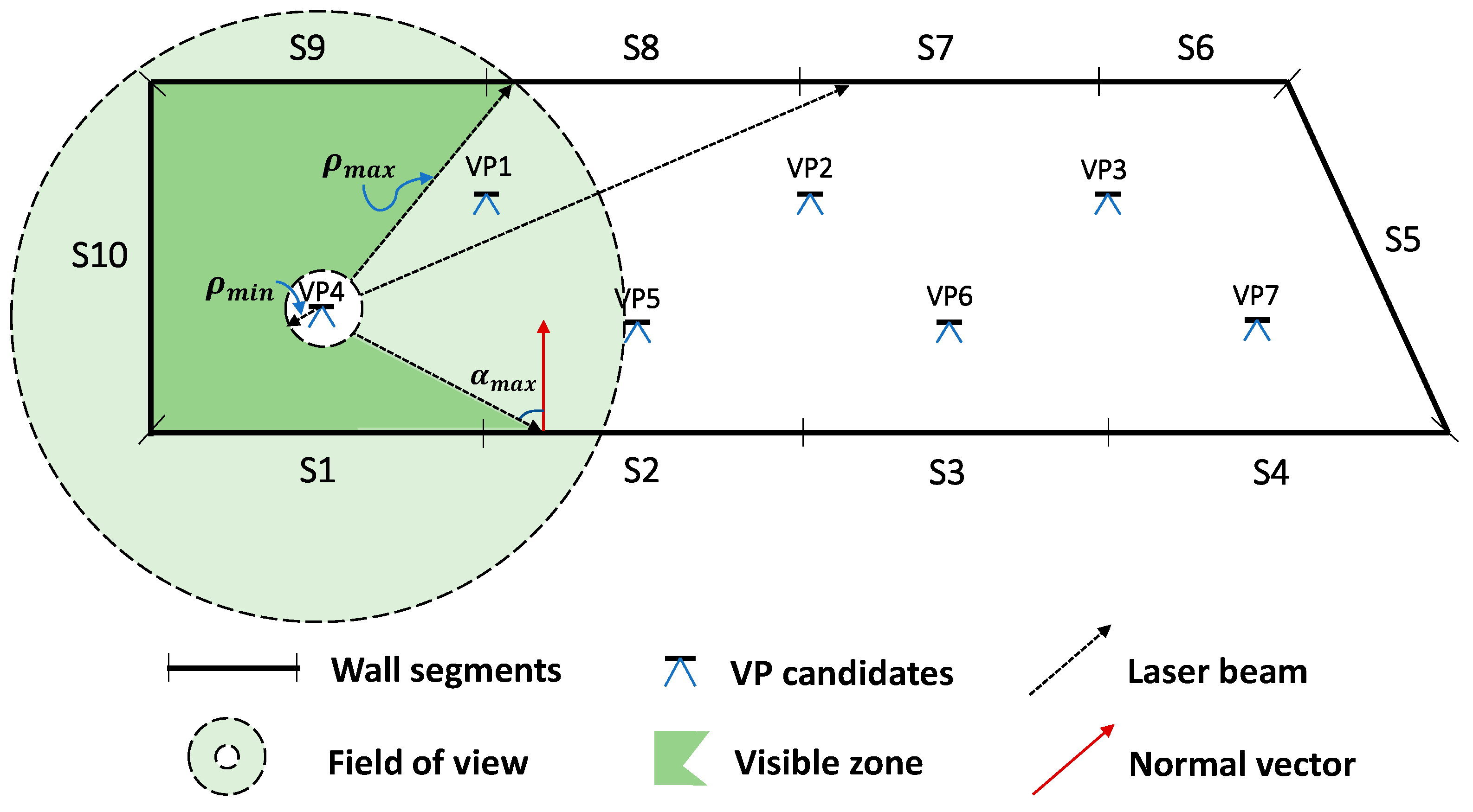
• Workspace: As described earlier, it is the space in which the instruments can be placed. Here, it is more precisely defined as global workspace and local workspace. The global workspace is the space around/within the scanning object. The local workspace is a specific local area within the global workspace;
• Candidate space: This is the set that contains all the created VP candidates;
• Resolution: If we consider the workspace as an image and the VP candidates as pixels, then the density of the VP candidates represents the resolution of the workspace. The smaller the step length between adjacent candidates is, the higher the resolution of the workspace will be. In the remaining of this paper, the increase of the resolution is realized by decreasing the step length;
• Optimal VPs: They are the VPs selected by the optimization methods, i.e., the GA or the WGA;
• Neighbourhood: A user-defined buffer around an optimal VP. In this research, the buffer is determined as a circle with a radius that is three times the resolution;
• Distinguishable VPs: Optimal VPs that have no other optimal VPs within their neighbourhoods;
• Indistinguishable VPs: Optimal VPs that have one or more other optimal VPs within their neighbourhoods.

In the hierarchical viewpoint planning strategy, the candidate space is constructed with a multi-scale principle, which starts at a course global resolution and continues with successively increased resolution. Local resolution is increased in the local workspace defined by a group of indistinguishable VPs. The candidate space is updated with the increase of the local resolution, and the optimal VPs are regenerated successively. This process repeats until all optimal VPs are labelled as distinguishable VPs.

The reason we proposed this strategy is that for distinguishable VPs, there are no other optimal VPs nearby, which makes this VP necessary and “dominate” the coverage of one part of the scanning object. Thus, increasing the local resolution does not help reduce the number of optimal VPs. On the contrary, indistinguishable VPs are spatially close to each other and tend to cover the same parts of the object. In this case, if their local resolution is increased, a solution with a smaller number of necessary VPs is likely to be found. The pseudocode of the proposed hierarchical viewpoint planning strategy is shown as follows.

1:    Input: a global workspace $W$

2:    Output: a set of optimal VPs $\mathcal{S}=\left\{V{P}_i|i=1,\dots ,m\right\}$

3:    Initialization:

4:       $r_0$: a course global resolution

5:       $c{s}_0$: candidate space under $r_0$

6:       $s_0$: a set of optimal VPs in $c{s}_0$

7:       $\mathcal{S}\leftarrow s_0$

8.    While VPs in $\mathcal{S}$ are not all distinguishable

9:       $r_i$: increase the local resolution

10:       $c{s}_i$: update candidate space

11:       $s_i$: find optimal VPs in $c{s}_i$

12:       $\mathcal{S}\leftarrow s_i$

13:     End

The process of the hierarchical strategy is summarized by the following steps:

• Initialization. The process starts from a course global resolution. With a relatively large step length, an initial candidate space with a small number of VP candidates is constructed. After the visibility evaluation, the proposed weighted greedy algorithm finds an initial set of optimal VPs in the initial candidate space;
• Label VPs. The optimal VPs are labelled as distinguishable/indistinguishable VPs based on their distance with other optimal VPs;
• Increase local resolution. After step 2, several groups of indistinguishable VPs that falls within a distance threshold is found. In this paper, the distance threshold is set as three times the current step length. A local workspace is defined for each group and the local resolution is increased by decreasing the current step length to half of it to obtain a partially denser candidate space. The local workspace is defined by extending the boundaries that surrounds the group of indistinguishable VPs with the current step length;
• Update optimal VPs. The weighted greedy algorithm provides new set of optimal VPs in the new candidate space;
• Stop criterion. Repeat steps 2 to 4 until all the optimal VPs are labelled as distinguishable VPs.

The traditional method and our proposed method for viewpoint planning, named Pipeline 1 and Pipeline 2, respectively, are summarised in

Table 3. Pipelines of two different strategies.

	Pipeline 1: Previous Methodology	Pipeline 2: Proposed Methodology
Candidate space construction	Uniform resolution	Hierarchical resolutions
Optimization method	GA	WGA

. In our method, the candidate space is constructed with the hierarchical, multi-scale strategy, in which the optimal VPs are searched by applying the improved weighted greedy algorithm. Two benefits of our proposed strategy are:

• Minimal VPs. The reduced number of optimal VPs is realized by two improvements. One is by reordering the priorities of VP candidates with the proposed weighted greedy algorithm. The other is by relocating indistinguishable VPs to more precise locations;
• High computational efficiency. Computational savings are realized from the hierarchical strategy that increases resolutions only at local workspaces of interest. It saves time by not evaluating a large number of unnecessary candidates, which is the case when the candidate space is constructed by the uniform resolution.

4. The Design System for the Target Placement

To link separate point clouds from multiple scans as a complete one, targets are utilized for the scan registration in this research due to the reason introduced in Section 2.2. In this section, our proposed target placement system is described. First, the general considerations in target arrangement are reviewed based on our evaluation criterion that is described in detail. The proposed strategy for target placement planning is then introduced as a four-step procedure.

4.1. Evaluation Criterion in Target Arrangements

As introduced in Section 2, the quality of registration is impacted by the distribution of targets. Some general rules should be followed:

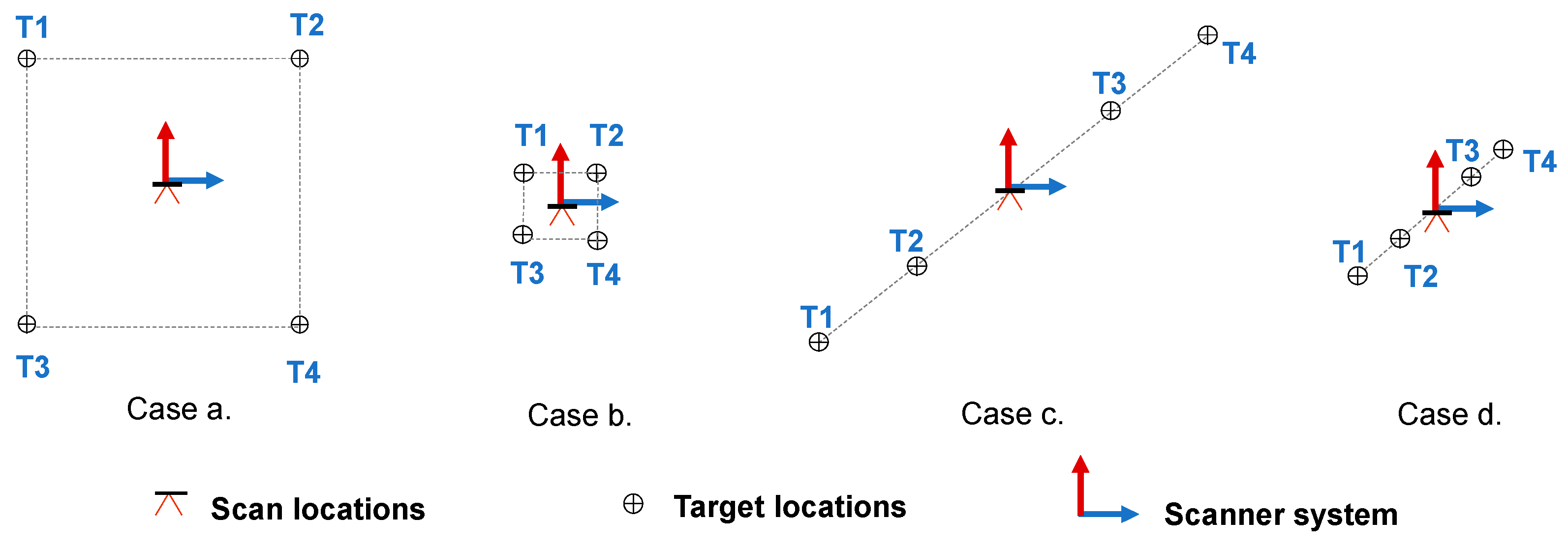
• Six coordinates from three targets observed from each scan, though the choice of which six coordinates is arbitrary, are the minimum requirements to solve for the registration parameters. This assumes that the scanner is not levelled. For the consideration of network reliability, at least four targets should be observed from each scan to provide redundancy;
• To maximize registration precision: 1) Targets should be distributed throughout the network volume, as far apart as possible; 2) targets that are collinearly or near-collinearly distributed are prohibited to avoid a singular system of equations.

The target placement problem can be stated as the minimization of the total number of the targets such that at least four targets can be observed from each optimal viewpoint, with the maximum precision of the registration parameters. It is notable that the target coordinates are pre-surveyed, so that each scan is georeferenced to the global frame when more than four targets are observed. In addition, an assumption is made that the scanning is set as high-resolution mode so that the targets can be captured precisely.

Instead of seeking the closed-form solution and the precision of the registration parameters, a simple criterion is sufficient to evaluate the target arrangement. It is well known that the spatial distribution of a set of points is captured by the covariance matrix of their coordinates. If the points are distributed linearly, the covariance matrix will be ill-conditioned. If the condition number of the covariance matrix in Equation (3) is used as the arrangement criterion of a target set ${\mathcal{S}}_t$, the better the distribution is, the smaller the condition number should be.

Criterion 1

$$f\left({\mathcal{S}}_t\right)=Cond\left(Cov\left({\mathcal{S}}_t\right)\right)$$

(3)

where $Cov\left({\mathcal{S}}_t\right)$ represents the covariance matrices of the coordinates of the target set ${\mathcal{S}}_t$, and $Cond\left(Cov\left({\mathcal{S}}_t\right)\right)$ means the condition number of $Cov\left({\mathcal{S}}_t\right)$, which is calculated as in Equation (4).

$$Cond\left(Cov\left({\mathcal{S}}_t\right)\right)=\Vert Cov\left({\mathcal{S}}_t\right)\Vert ·\Vert Cov{\left({\mathcal{S}}_t\right)}^{-1}\Vert$$

(4)

where $\Vert ·\Vert$ means the norm of the matrix.

Criterion 1 is tested on the four types of targets arrangements shown in Figure 2. Based on the target arrangement considerations, the values from the evaluation criterion for these four cases should be $f\left(a\right)<f\left(b\right)<f\left(c\right)<f\left(d\right)$. However, from Equation (3), the values are $f\left(a\right)=f\left(b\right)<f\left(c\right)<f\left(d\right)$, which means the criterion is not capable of find the discrepancy between Case a and Case b. To distinguish these two cases, we use the area of the polygon defined by the target set ${\mathcal{S}}_t$, $S_{{\mathcal{S}}_t}$, to normalize the condition number, which led to the new criterion.

Criterion 2

$$ℱ\left({\mathcal{S}}_t\right)=\frac{f\left({\mathcal{S}}_t\right)}{S_{{\mathcal{S}}_t}}=\frac{Cond\left(Cov\left({\mathcal{S}}_t\right)\right)}{S_{{\mathcal{S}}_t}}$$

(5)

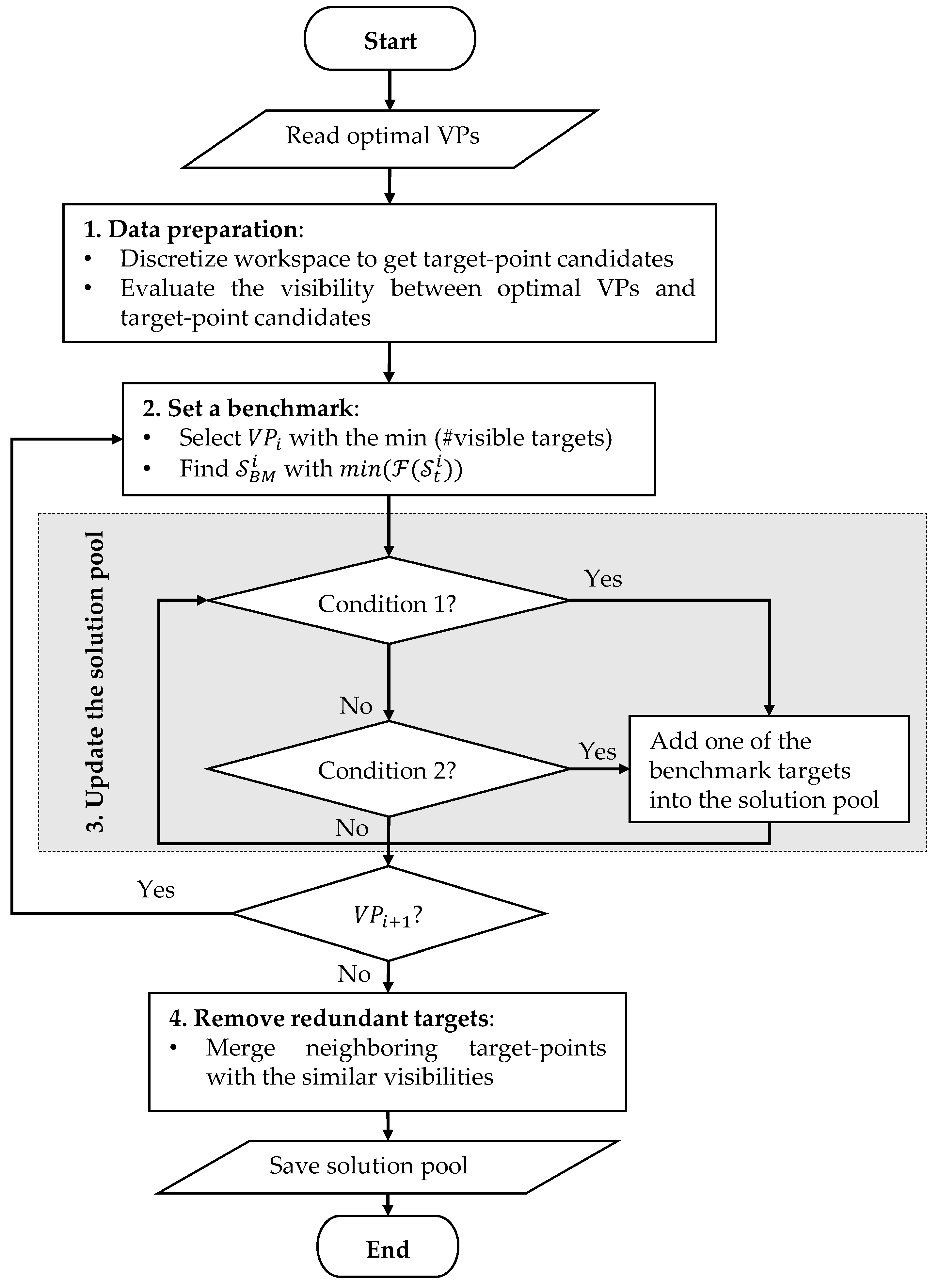
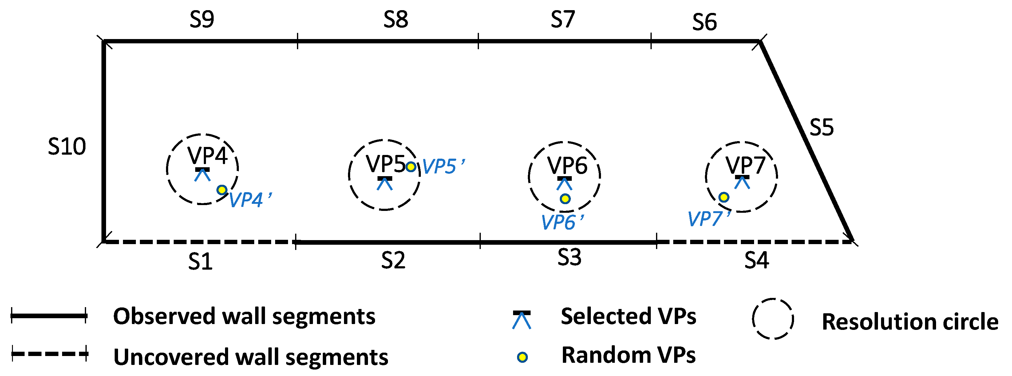
4.2. Procedure of the Target Placement Planning

The planning of target placement is determined with a two-fold pipeline. First, targets are selected viewpoint by viewpoint. Afterwards, the set of all selected targets is analysed and “trimmed”. The procedure to obtain the target placement for the entire network comprises the following steps.

1.  Data preparation

In this step, the target-point candidates are created by discretizing the workspace with a uniform resolution. In this paper, we use the word target-point to represent the locations for targets, similar to the viewpoint for the scanner placement. The visibilities of the target-point candidates from the optimal VPs are evaluated to obtain the visible target pool for each VP.

2.  Set a benchmark

The method starts from the optimal VP that observes the minimum number of target-point candidates and sets a benchmark geometry for its target distribution. The process of determining the benchmark geometry is to select four random visible target-point candidates in an iterative manner and calculate the criterion based on Equation (5). The target set with the minimum criterion is recorded as the benchmark geometry, represented by ${\mathcal{S}}_{BM}^i$, for the ith optimal VP. This benchmark geometry is not the final design for the target-points. Instead, it will be used as a guide in planning the target placement.

3.  Get/Renew the solution pool

The solution pool represents the set that contains all the selected target-points. It gets updated after processing each viewpoint. For each optimal VP, the benchmark target-points are the candidates to update the solution pool. When processing the first optimal VP, the four target-points in the benchmark geometry are added into the solution pool directly. For N VPs, there should be $4\times N$ target-points if all the benchmark target-points are added into the solution pool. In other words, the maximum size for the solution pool is $4\times N$. However, VPs that are picked later than others might be able to observe the existing target-points in the solution pool. When the existing target-points can provide the similar geometry with the benchmark geometry, it gives the possibility to reduce the size of the solution pool.

The intersection between the visible target pool of each VP and the existing solution pool is represented by:

$${\mathcal{S}}_{vt}^i\cap {\mathcal{S}}_s^{i-1}=\left\{t_1,\dots ,t_n\right\}$$

(6)

where ${\mathcal{S}}_{vt}^i$ represents the visible targets pool for the i^th optimal VP; ${\mathcal{S}}_s^{i-1}$ is the solution pool after processing the last $i-1$ optimal VPs; $t_1,\dots ,t_n$ are the $n$ targets in the intersection of the two sets.

After processing each optimal VP, the solution pool will be renewed if one of the following two conditions are satisfied.

Condition 1

There are less than four visible target-points in the intersection, which means that the set of visible target-points in the solution pool is not sufficient for scan registration.

$${\mathcal{S}}_{vt}^i\cap {\mathcal{S}}_s^{i-1}=\left\{t_1,\dots ,t_n\right\} n<4$$

(7)

Condition 2

There are more than four visible targets in the intersection, but the geometry of the visible targets in the solution is not competitive with the benchmark geometry. In Equation (8), the geometry of the intersection is not competitive when its criterion is more than three times the benchmark geometry.

$$\{\begin{array}{l}{\mathcal{S}}_{vt}^i\cap {\mathcal{S}}_s^{i-1}=\left\{t_1,\dots ,t_n\right\} n\ge 4\\ ℱ({\mathcal{S}}_{vt}^i\cap {\mathcal{S}}_s^{i-1})/F\left(S_{BM}^i\right)>3\end{array}$$

(8)

Under either of the above two conditions, the target-points in the benchmark geometry will be included in the solution pool one by one until both conditions fail. After the target-points are determined for $V{P}_i$, the method moves to $V{P}_{i+1}$, then step 2 and step 3 are repeated until all the optimal VPs are assessed.

4.  Remove redundant targets

In the solution pool, some VPs might observe more than four targets. An extra operation is for the removal of redundant targets. The principle is to check if neighboring targets have similar visibilities. If two target points are close with each other, and they can be observed from the same VPs, the one that is observed from fewer VPs is “trimmed” as long as at least four targets are still observed by each VP.

With the above four steps, the final solution with the minimum number of target-points is provided. Figure 3 is the flowchart of the proposed target placement method.

The benefits of our method are:

• High quality. This reflects in both the registration precision and the redundancy of the network. The registration precision is preserved by determining the target-point layout under the guide of the benchmark geometry; and the redundancy is satisfied when at least four targets are observed from each viewpoint location;
• Minimal targets. With no prejudice to the network redundancy, the number of the selected target-points is minimized in two ways. One is by accepting the existing target-points in the solution pool whose geometry is competitive with the benchmark geometry; the other one is to “trim” the target-points that are inferior to the other target-points in the final step.

5. Quality Assessment

In this section, the quality assessments of the solutions, regarding both the sensitivity of the object coverage to the scanner placement and the numerical precision of the point clouds, are investigated.

5.1. Sensitivity Test of the Scanner Placement

The designing goal in the scanner placement stage is that the maximum coverage of the object scanning scene is achieved by the selected optimal VPs. Due to some reasons that are not considered in the design, e.g., the occlusions from some random vehicles or plants, users are not always able to place all the VPs at their optimal locations in the field, which impacts the maximum coverage of the scanning scene from the design. The sensitivity of the object coverage to the actual placement of the VPs is tested in this research.

In this research, the sensitivity of the solution specifically means how sensitive the coverage rate of the object is to the actual placement of the viewpoints. The coverage rate of the scanning scene is used to assess the sensitivity of the solution. This indicator $E$ is calculated as:

$$\mathrm{Coverage}\mathrm{rate}(\%):E=\left(N_{obs}/N_{all}\right)\ast 100$$

(9)

where $N_{obs}$ represents the number of wall segments observed from the selected VPs, and $N_{all}$ is the number of all the discretized wall segments. The coverage rate should be 100% since the maximum coverage is required.

The process to test the sensibility is by simulating $n$ sets of random solutions. For each optimal VP from the hierarchical strategy, the random VPs are generated within a circle, whose radius is the resolution when the optimal VP was labelled as distinguishable VP in Section 3.2. For the example in Figure 1, VP4, VP5, VP6, and VP7, are four viewpoints selected by the proposed method to provide a 100% coverage of the object. In Figure 4, VP4’, VP5’, VP6’, and VP7’, are a set of random VPs, from where S1 and S4 are not covered due to the incidence angle constraint. In this case, the coverage rate of the random solution is calculated as 80% based on Equation (9).

In the process of repeating $n$ times, the coverage rates of these new solutions are recorded. With this information, the field crew can have a better knowledge about how careful they should be in placing the scanner for data collection. The result also indicates how many times each wall segment is not covered in the tests. This provides a tool to probe the sensitive parts of the network where the user should pay more attention to.

5.2. Precision Measure of the Scanning Object

In target-based registration, the typical convention is to treat the target coordinates as constant quantities, thereby removing them as unknowns from the registration problem. Thus, once the placement for viewpoints and target-points are achieved, we can estimate the object-space coordinates of each individual point in the registered point cloud, by projecting the observed scan-space coordinates of each point using the registration parameters of each scan. For a point $p_i$ observed from viewpoint j, the transformation model for the projected object point $P_i$ is:

$$P_i=R_j^T{p}_{ij}+T_j$$

(10)

where $R_j^T$ is the rotation matrix expressed as a function of three rotation parameters $\left({\omega }_j, {\phi }_j, {\kappa }_j\right)$ and $T_j$ is the vector ${\left[X_j,Y_j,Z_j\right]}^T$ comprising three translation parameters, from scan j to the object space. According to the design, each object point in the point cloud should be observed from at least one viewpoint. For the sake of presentation clarity in the point precision, each object point is assigned with a master viewpoint, from where the effective scanning distance is the closest.

Based on the error propagation rule, the covariance matrix for the project point $P_i$ in Equation (11) is impacted by three sets of variables: The observations, the registration parameters, and the additional parameters.

$$C_{P_i}=\frac{\partial P_i}{\partial {\ell }_{ij}}{C}_{{\ell }_{ij}}{\frac{\partial P_i}{\partial {\ell }_{ij}}}^T+\frac{\partial P_i}{\partial x_j}{C}_{x_j}{\frac{\partial P_i}{\partial x_j}}^T+\frac{\partial P_i}{\partial x_a}{C}_{x_a}{\frac{\partial P_i}{\partial x_a}}^T$$

(11)

${\ell }_{ij}$ is the spherical coordinate observation for point i from viewpoint j, which is a vector consists of range ${\rho }_{ij}$, horizontal orientation ${\theta }_{ij}$, and vertical orientation ${\alpha }_{ij}$; $x_j$ is the vector of registration parameters, and $x_a$ is the vector composed of four additional parameters, the rangefinder offset $a_0$, the collimation axis error $b_1$, the trunnion axis error $b_2$, and the vertical circle index error $c_0$. $C_{x_j}$ is the covariance matrix of viewpoint j’s registration parameters; $C_{{\ell }_{ij}}$ is the observation covariance matrix for point i in viewpoint j; and $C_{x_a}$ is the covariance matrix of the additional parameters.

The partial derivatives in Equation (11) are the Jacobian matrices of $P_i$ in terms of the three sets of variables, which can be derived from Equation (10). Assuming uncorrelated observation errors, the $3\times 3$ covariance matrix for each point observation is diagonal with the form of:

$$C_{{\ell }_{ij}}=\left[\begin{array}{ccc}{\sigma }_{\rho }^{2}se{c}^2{\beta }_{ij}& 0& 0\\ 0& {\sigma }_{\theta }^2& 0\\ 0& 0& {\sigma }_{\alpha }^2\end{array}\right]$$

(12)

where ${\sigma }_{\rho }^2$, ${\sigma }_{\theta }^2$, and ${\sigma }_{\alpha }^2$ are the variances for range with the normal incidence, horizontal, and vertical angles, respectively. For the range error, the incidence angle of the laser beam ${\beta }_{ij}$ is considered by including the $se{c}^2{\beta }_{ij}$ term.

The covariance matrix $C_{x_j}$ for the registration parameters of scan j is estimated through the target-based registration. All additional parameter errors are also assumed to be uncorrelated, which gives the $4\times 4$ covariance matrix with the form of:

$$C_{x_a}=\left[\begin{array}{cccc}{\sigma }_{a_0}^2& 0& 0& 0\\ 0& {\sigma }_{b_1}^2& 0& 0\\ 0& 0& {\sigma }_{b_2}^2& 0\\ 0& 0& 0& {\sigma }_{c_0}^2\end{array}\right]$$

(13)

where the diagonal elements represent the variances for four main systematic error sources. The additional parameters and their covariance matrix are assumed to be pre-determined in a laboratory-based self-calibration.

With all the above parameters, the covariance matrix for each projected point in Equation (11) can be calculated. Then, the semi-major axis of the 95% confidence ellipsoid is obtained by extracting and scaling the largest eigenvalue and is used as the precision measure of each object point. The precision of the scanning object can be estimated as the indicator of our network design system, to ensure that the project specifications are satisfied.

6. Experiments and Discussions

In this section, our methodologies were applied on two cases, one indoor and one outdoor environment, and the quality assessments were implemented to illustrate the sensitivity of the solution and the quality of the point cloud. All methods are conducted on an Intel^® Core^TM i5-7500, 3.40 GHz, 24 GB RAM computer, and implemented by using C++ in the Microsoft Visual Studio 2017 environment.

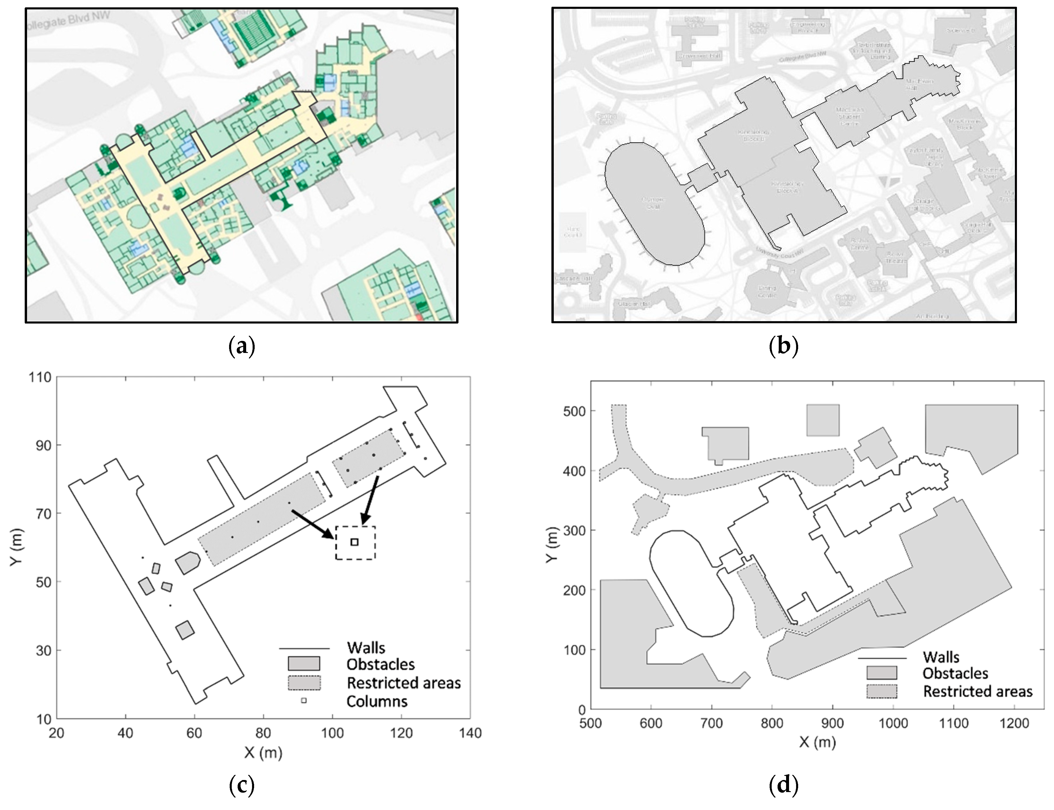
6.1. Experimental Environments

The experiments were performed on two datasets, both of which are located on the University of Calgary campus. The objects were extracted from publicly available 2D floor maps from the University of Calgary website. The datasets are illustrated in Figure 5. Figure 5a is the indoor case for the main floor of the MacEwan Student Centre. Figure 5b is the outdoor case, which is a multi-use complex starting from the Olympic speed skating Oval at the most southwest side, to the MacEwan Student Centre at the northeast corner. The areas of interest for the data simulation are outlined.

The simulation data extracted for the experiments are shown in Figure 5c,d. The objects are marked by the connected or independent black lines, representing the building façades or interior walls, which will be discretized into the wall segments in the experiments. The grey shaded areas denote inaccessible zones for the placement of viewpoints or target-points. Obstacles occluding the laser rays, e.g., statues or buildings, are outlined with solid black lines. The laser ray can pass through restricted areas such as the dining area in the food court, i.e., grey shaded area in Figure 5c, or roads around the building in Figure 5d. These areas are outlined with black dashed lines. All other white-coloured areas are the workspace for viewpoint or target-point candidates. The workspace defined in the simulation is assumed to be safe and stable for instrument placements.

The meta-data of the experimental datasets are listed in

Table 4. Meta-data of the experimental datasets.

	MacEwan Student Centre	Oval-MacEwan Complex
Environment	Indoor	Outdoor
Dimensions	120 m × 90 m	700 m × 500 m
# Walls	93	259
Unit length	1 m	2 m
# Wall segments	630	1182

. The network volume for the MacEwan Student Centre is relatively small, with 630 wall segments and the dimension of around 120 m × 90 m. Both square and round columns are discretized into square elements and their modelling is considered as sufficient if more than two faces are visible from the selected scanner locations. The Oval-MacEwan complex has a larger volume, with 1182 wall segments and the dimension of around 700 m × 500 m, and its surrounding environment is more complex with neighbouring buildings and driveways.

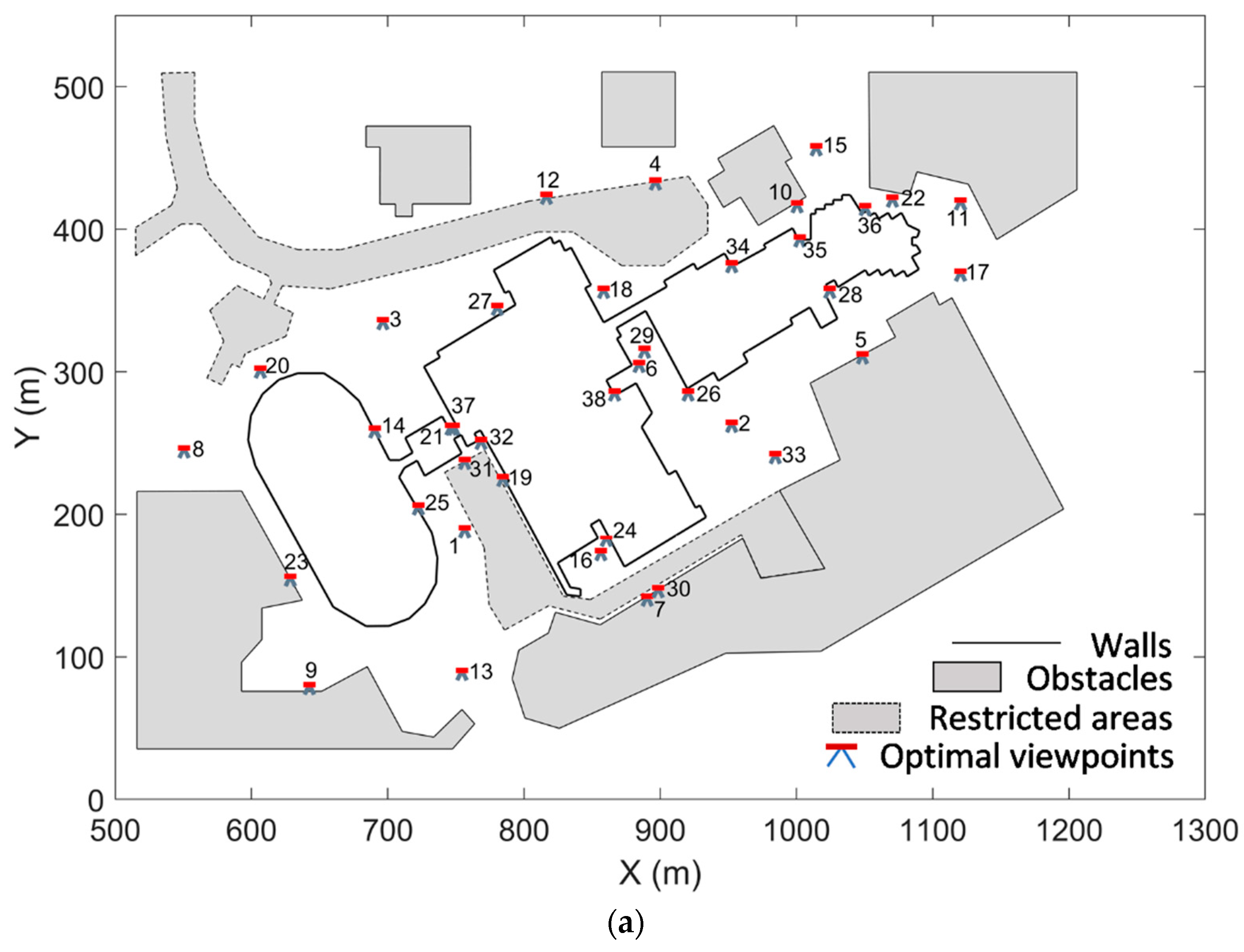
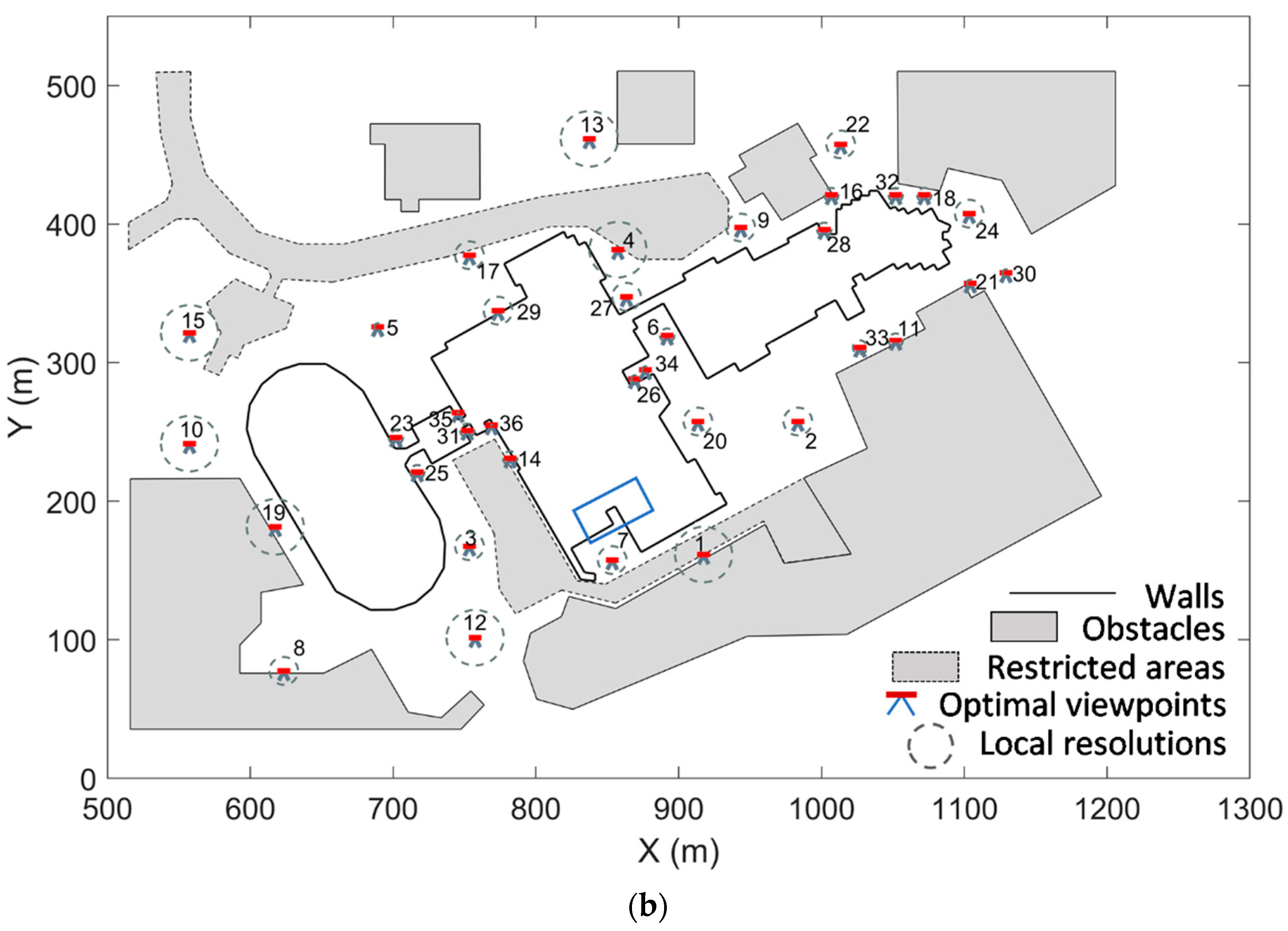
6.2. Designs for the Scanner Placement

The two pipelines introduced in Section 3, “Uniform resolution + Greedy Algorithm” (Pipeline 1) and “Hierarchical resolutions + Weighted Greedy Algorithms” (Pipeline 2), were applied on each dataset. Their performance in terms of the number of the selected viewpoints and program runtime are compared.

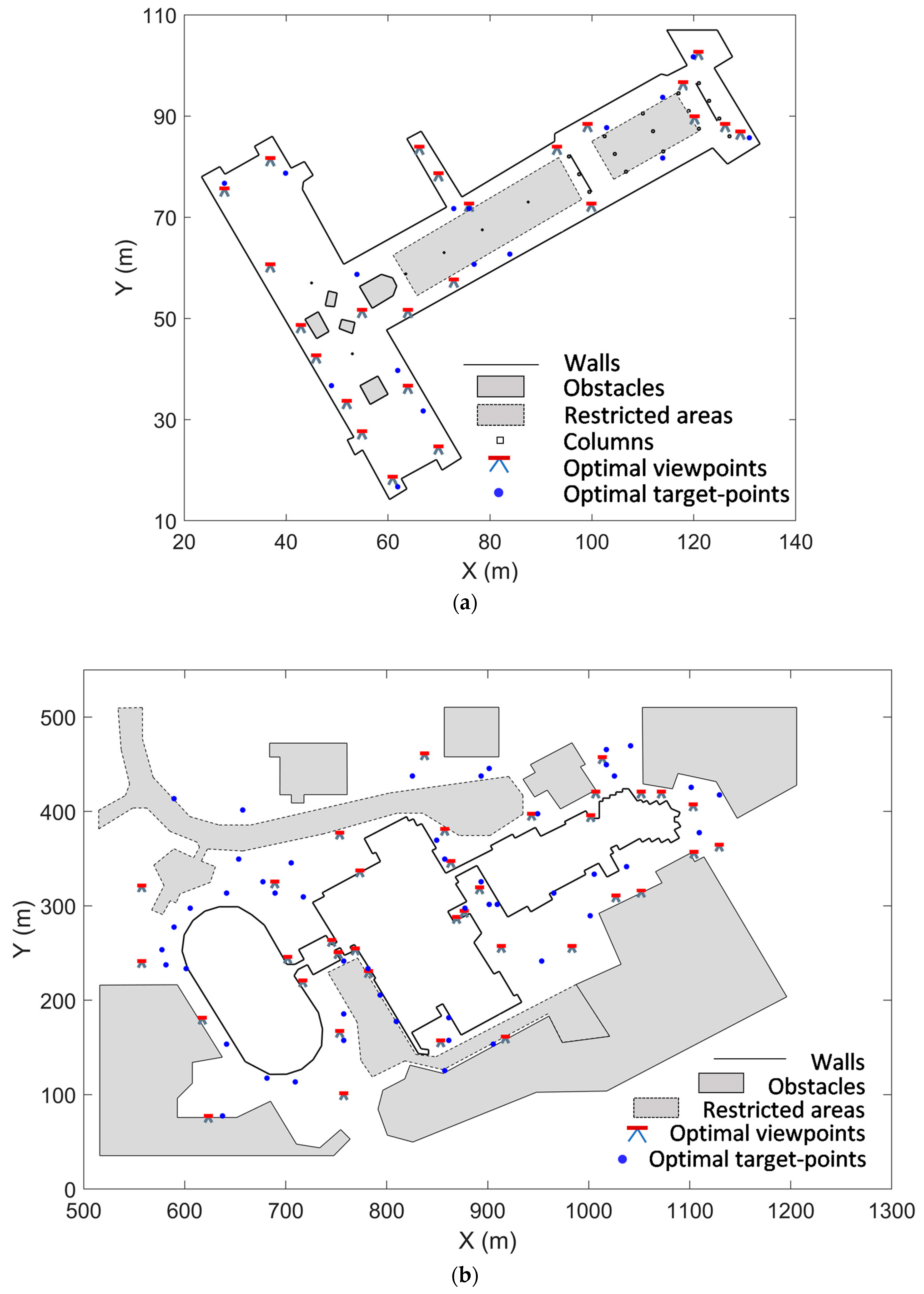
6.2.1. MacEwan Student Centre

The solutions from two pipelines are illustrated in Figure 6. Figure 6a shows the solution from Pipeline 1, for which the VP candidates were constructed globally with the uniform resolution of 1 m. The solution comprises 28 VPs selected from 855 VP candidates. In Figure 6b, 24 VPs were selected from our proposed Pipeline 2, with four VPs less than the Pipeline 1 solution and a complete object coverage. Each optimal VP is circled with the radius of the resolution when this VP is labelled as a distinguishable VP. One can tell how the hierarchical progress works from the various radii. In this dataset, the construction of VP candidates started with the initial resolution of 4 m. Several of the VPs were labelled as indistinguishable VPs, e.g., VP17 and VP21, the resolution for these local areas was increased to 2 m, while VPs like VP1, VP5, and VP12, were saved as distinguishable VPs under the resolution of 4 m. Finally, the progress ended at the finest local resolution of 1 m, where VP23 and VP24 were selected as the last two distinguishable VPs.

The performance of the two pipelines is summarized in

Table 5. Comparison of the performance of two pipelines on the experimental datasets.

	MacEwan Student Centre		Oval-MacEwan Complex
	Pipeline 1	Pipeline 2	Pipeline 1	Pipeline 2
Resolution	1 m	1 m (4 m)	2 m	0.035 m (20 m)
# VP candidates	855	167 (122)	25,268	1873 (1317)
# Selected VPs	28	24	38	36
Program runtime	~1.3 h	~0.25 h	~49 h	~3.9 h
Coverage rate	100%	100%	100%	99%

. In the first row, the table lists the resolution applied in two pipelines, while the number in the bracket for Pipeline 2 represents the course global resolution that the program starts from. The total number of VP candidates is shown in the second row. By using Pipeline 2, for the MacEwan Student Centre dataset, there were 122 VPs created at the course resolution and the program finished when this number increased to 167 VPs. The program runtime is compared in the third row. For the MacEwan Student Centre dataset, the runtime is reduced from 4730 s (~1.3 h) to 904 s (~0.25 h), which represents an 80% improvement. The full coverage is achieved in both methods.

6.2.2. Oval-MacEwan Entertainment Complex

The scanner placement for the Oval-MacEwan complex dataset is illustrated in Figure 7. For results from Pipeline 1, 38 optimal locations were selected from 25268 VP candidates at the resolution of 2 m, with the 100% coverage of the object. In Figure 7b, 36 viewpoints were selected from Pipeline 2, with the resolutions increasing from 20 m to 0.035 m. The coverage rate of the object is 99%, and the missing area is at the corner near to VP7. The reason for the incomplete coverage is the lack of viewpoints, since no VP candidates are created in this narrow space. This is a limitation of the hierarchical method, that the initial resolution should be selected carefully otherwise certain areas would not be observed from any of the VP candidates. The missing part of the object is shown in the sensitivity tests in Section 6.4, where the users can manually add extra scans to complete the object coverage.

In this case, the advantage of our proposed method in the number of viewpoints is less obvious, especially after adding extra scans at missing area. However, the main benefit is the improvement of efficiency in the planning of the scanner placement. It takes about 49 h, which is more than two days, to evaluate and select optimal VPs with Pipeline 1, while less than four hours are required with Pipeline 2. The improvement is more than 92%. In terms of computational efficiency, this is a worthwhile trade-off. For example, if the original design cannot be executed due to some conditions that are not considered, by adding a few constraints, it can be quickly re-designed within a short re-run time.

6.3. Designs for the Target Placement

Using the method introduced in Section 4, the target placement was determined. For the MacEwan Student Centre dataset, target-point candidates were created with the uniform resolution of 1 m, while for the Oval-MacEwan Complex dataset, the step length was 2 m. The visibilities between the target-point locations and optimal VPs were tested based on the scanning geometry, with the minimum range of 2 m and the maximum range of 100 m. The target placement for the two datasets are illustrated in Figure 8. Sixteen target-point locations were finally selected for the MacEwan Student Centre case in Figure 8a, while 49 target-point locations were required for the Oval-MacEwan Complex case in Figure 8b. The program finished in 12 s and 41 s for the MacEwan Student Centre and the Oval-MacEwan Complex datasets, respectively, when 3000 iterations were set to determine the benchmark geometry.

Among the target placement, at least four targets were observed from each scan, with an optimal geometry described in Section 4.1. In our method, the attribution of each selected target location is provided, indicating which four (or more than four) target locations are necessary for each scan. This means the users need to prepare only a few targets to accomplish the entire scanning project.

It is noticeable that some target locations are distributed near-collinearly with the scans, e.g., the three targets and seven scans that placed along with the west-most walls in Figure 8a. In this case, if more than one target is arranged along the same line of sight from a scan, we need to avoid vision obstacles by adjusting target heights.

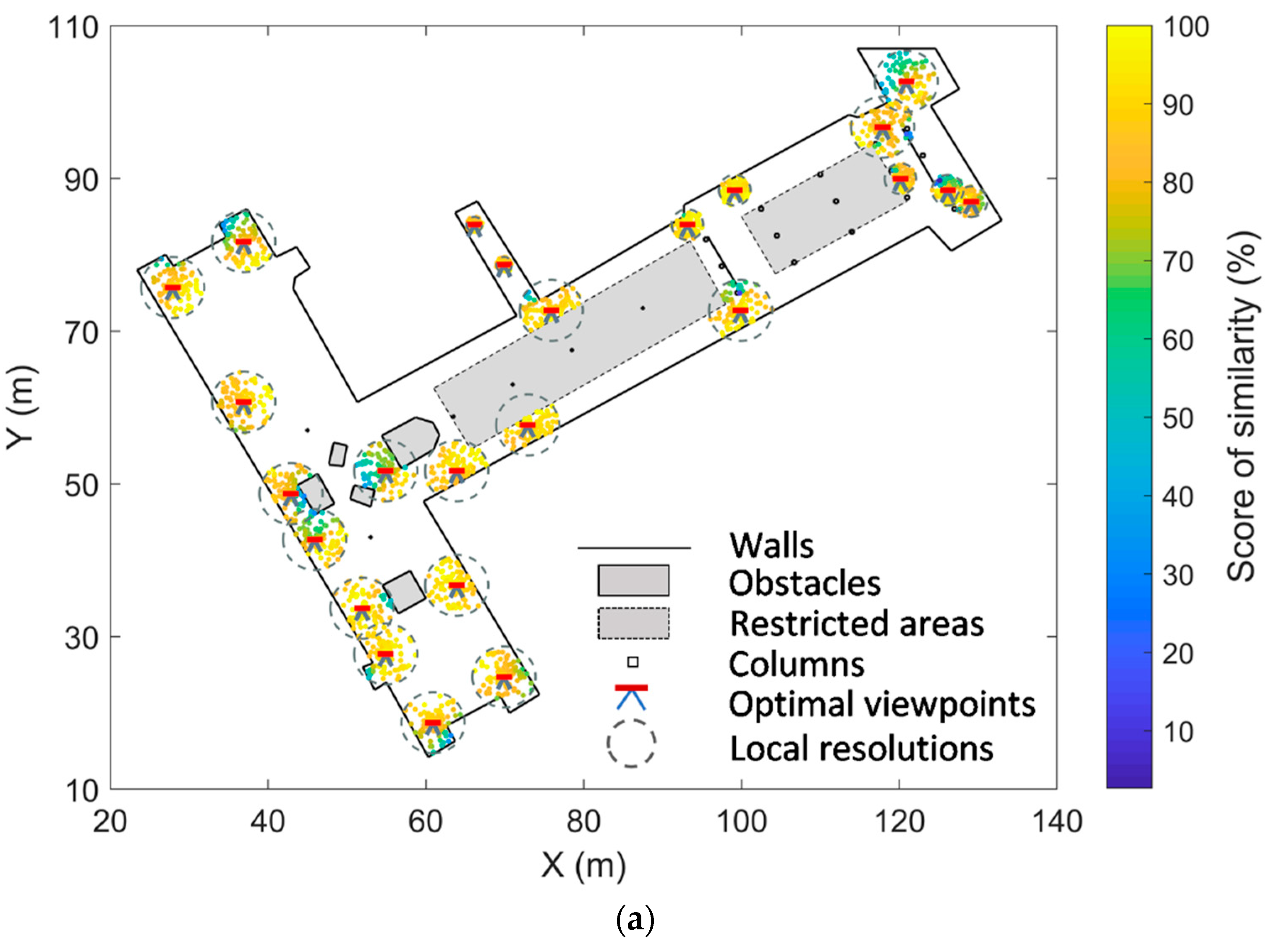
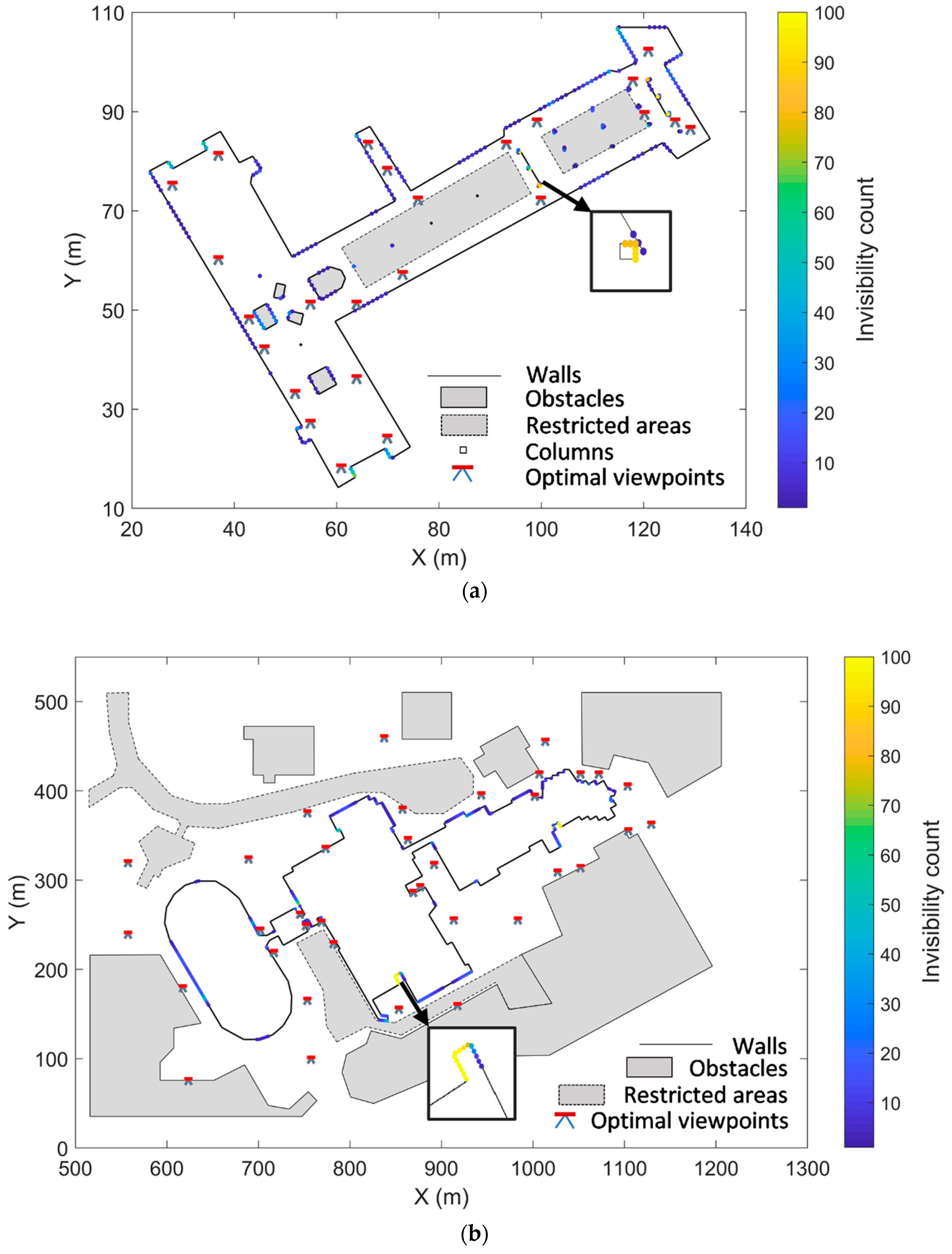
6.4. The Sensitivity Tests

In the experiments for the sensitivity tests, we created 100 different solutions within their corresponding resolution circles, as shown in Figure 9. The colour of each point represents the score of similarity to its optimal location. The scores are calculated as the percentage of the visible segments from the optimal location that is covered by the random points. A higher score means the coverage of the random viewpoint is more similar with its optimal location, which is represented by yellow dots. These heatmaps help users choose the alternative scan location when the optimal planned placement is not available.

We calculated the average coverage rates of the 100 random solutions from Equation (9). Over the 100 cases, the average coverage rates for both datasets are around 96%. With this information, the field crew can have a better knowledge about how careful they should be when placing the scanner for data collection.

We also counted the number of times that each wall segment was not observed in the 100 tests. The colour in Figure 10 indicates the invisibility count. This provides another tool to probe the sensitive parts of the scanning object and indicates where the users need to take more care of. A count is zero preferred, which means that the coverage of that area is less sensitive to the change of the viewpoints.

One can see some areas with the higher invisibility count in both figures, as shown in the enlarged images, which are due to different reasons. For the MacEwan Student Centre case, as introduced, the columns are considered fully covered if more than two faces of the square model are scanned. In Figure 10a, two faces of the column are invisible due to the obstacle of the interior wall connected to it. For the Oval-MacEwan Complex dataset, the existence of invisible parts is because of the missing of viewpoints in the narrow area, as discussed in Section 6.2.2.

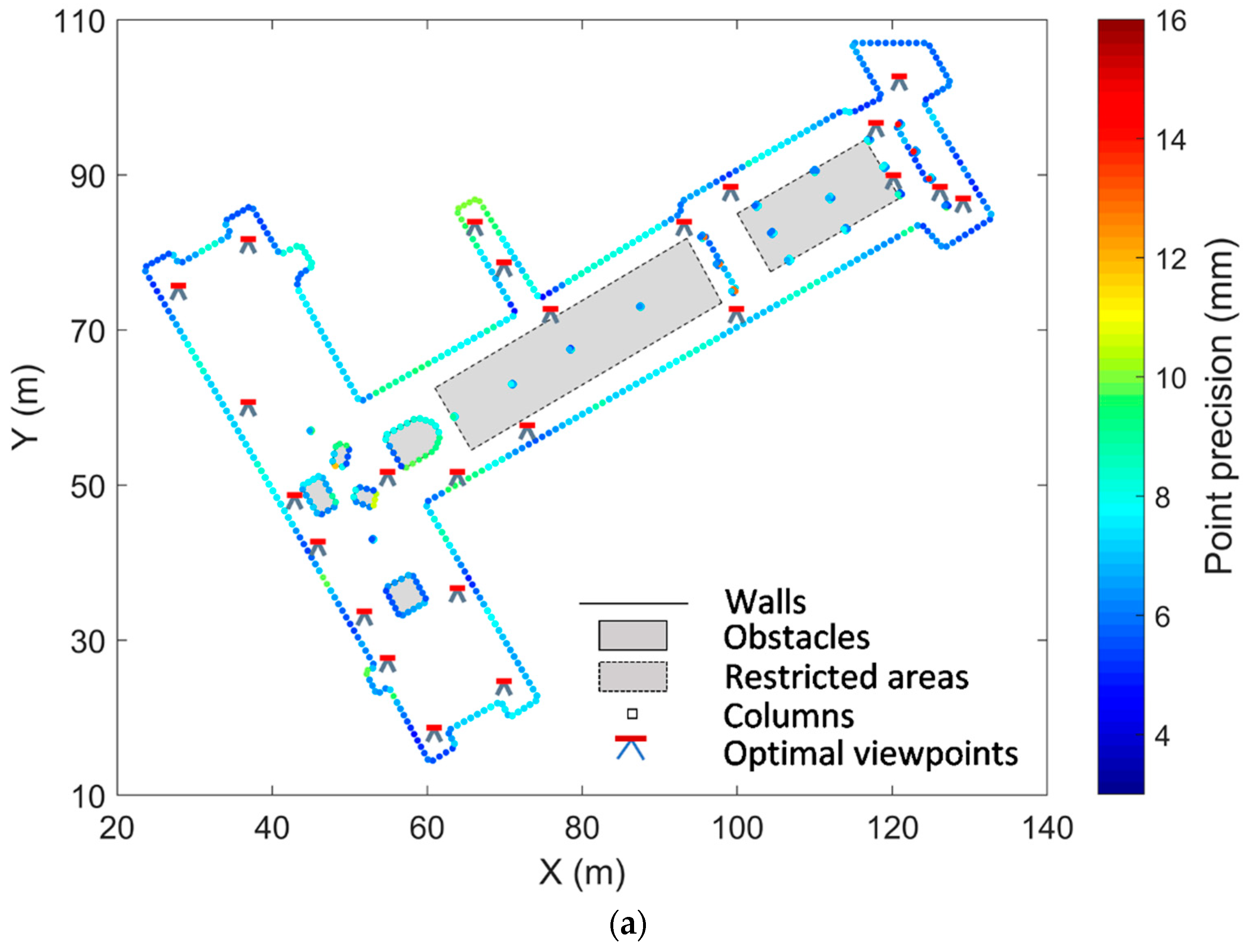
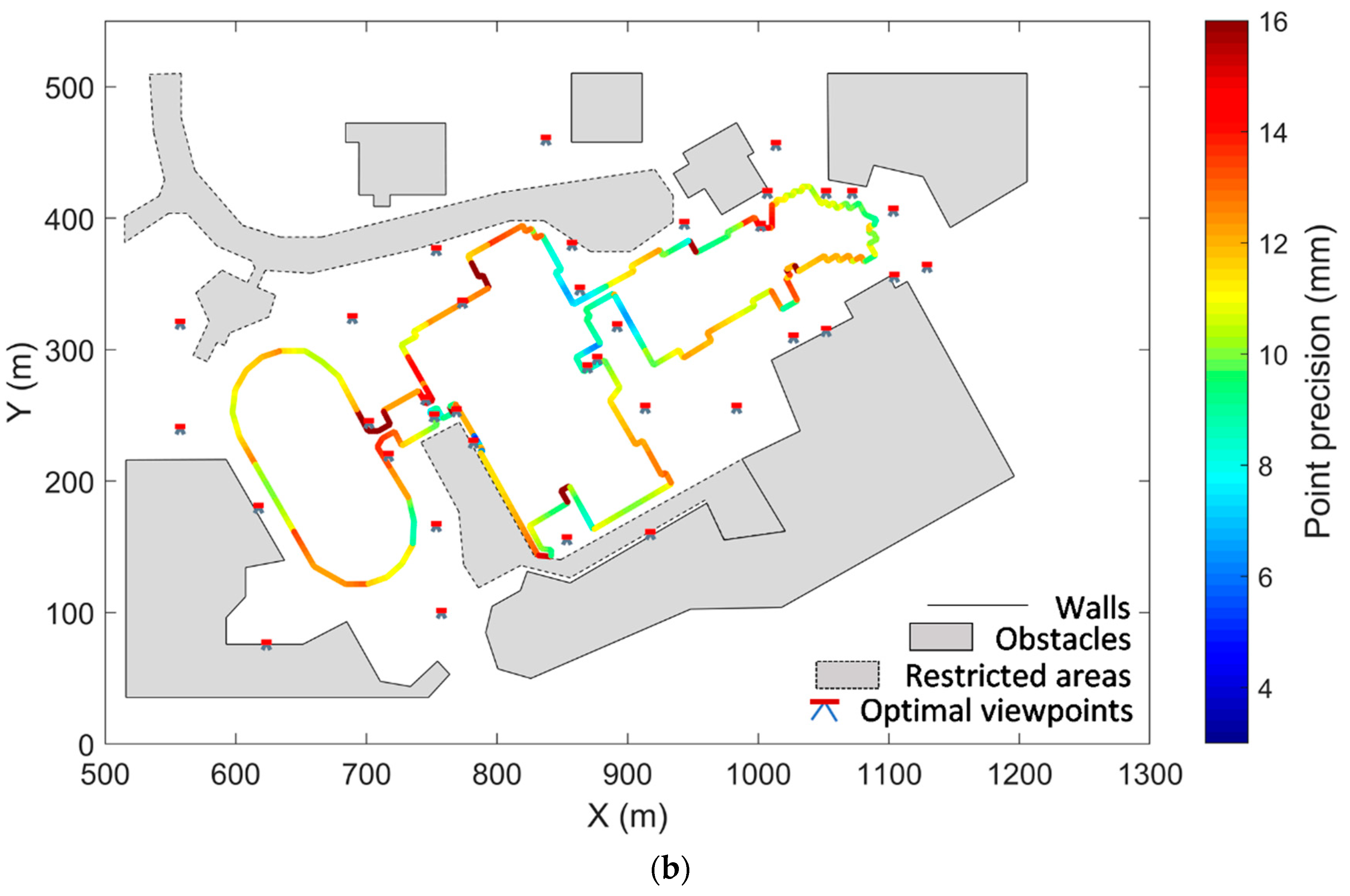
6.5. Point Cloud Precision

The covariance matrix of the projected point cloud was estimated through error propagation according to Equation (11). The simulated standard deviations for observations and additional parameters in this research are listed in

Table 6. Parameter precisions in the simulation.

Observations	${\sigma }_{\rho }$ (mm)				${\sigma }_{\theta }$ (″)				${\sigma }_{\alpha }$ (″)
	±1				±30				±30
Additional parameters	${\sigma }_{a_0}$ (mm)		${\sigma }_{b_1}$ (″)				${\sigma }_{b_2}$ (″)			${\sigma }_{c_0}$(″)
	±0.1		±10				±10			±10
Registration parameters	${\sigma }_{\omega }$ (°)	${\sigma }_{\phi }$ (°)		${\sigma }_{\kappa }$ (°)		${\sigma }_{\Delta X}$ (mm)		${\sigma }_{\Delta Y}$ (mm)			${\sigma }_{\Delta Z}$ (mm)
	±0.03	±0.03		±0.01		±6.9		±4.6			±7.9

. The precision simulated here are specific for this paper, which is drawn from experience using and calibrating TLS instruments [17]. The maximum standard deviations for the estimated registration parameters are also listed.

The overall point precision for the two datasets is shown in Figure 11. In Figure 11a, the single point precision for the MacEwan Student Centre dataset varies from ±3 mm to ±14 mm, with a root mean squared (RMS) value of ±7 mm. In the Oval-MacEwan Complex dataset in Figure 11b, the overall point cloud uncertainty falls into the range between ±5 mm to ±16 mm, with the RMS value of ±12 mm. One can see that the red-coloured parts with higher uncertainty in both figures are from the uncovered parts of the object due to the same reason discussed before. The largest contribution comes from the registration parameters. The existence of many restricted area and obstacles leaves limited space for the target placement. Thus, many targets are placed with either small area or not as good geometry, especially for scans placed at corners, which causes lower precision at points that are scanned from these scan locations. Overall, the point cloud precision of the MacEwan Student Centre dataset is mostly homogeneous. The precision of the Oval-MacEwan Complex dataset is heterogenous due to its longer sight lines and more complex shape.

7. Conclusions

In this paper, a model-based TLS network design system was proposed to aid the planning process for high-accuracy modelling of the large-volume objects. Our pipeline, the “Hierarchical resolutions + Weighted Greedy Algorithm” for the optimal scanner placement was introduced and compared with the traditional “Uniform resolution + Greedy Algorithm” pipeline. Comparison of the methods in two environments showed that the proposed pipeline provided compatible scanner placement solutions with more than 80% improvements in terms of computational efficiency.

For the target-point placement, our proposed method provided solutions with a high quality in terms of both the final point cloud precision and the network redundancy. Furthermore, the number of the selected target-points is minimized by accepting the close to optimal target arrangement. Considering the volume of the network, the number of necessary target-points from our design was surprisingly small.

Last but not least, the design quality was assessed in two aspects. One is the sensitivity of the solution to the placement of the scanner, which helps users to know the weak areas of the network regarding the object coverage. The other one is the point cloud precision, which let users interpret the quality of the point cloud and ensure the project specifications can be met.

The strategy has been developed without reference to a specific scanner system, which means that one can modify the constraints in planning according to the properties of different instruments, e.g., the range capacity including both the minimum and maximum range of the scanner, the scanning window, etc. In this research, the overlap between scans is not considered in the design, which limits the cloud-to-cloud registration using the ICP. Although we assumed that the scan resolution is set properly so that the targets can be captured precisely in this paper, the scan resolution is indeed an aspect that should be considered in the design. Also, this paper only presents the 2D approach as it provides a first insight of the design. The extension to 3D causes extensive computations. Finally, the algorithm requires further improvements so that the risk of incomplete reconstruction from the hierarchical design strategy can be reduced or completely avoided. These problems are expected to be solved in the future work.

References

1. Oskouie, P.; Becerik-Gerber, B.; Soibelman, L. Automated measurement of highway retaining wall displacements using terrestrial laser scanners. Autom. Constr. 2016, 65, 86–101. [Google Scholar] [CrossRef]
2. Maalek, R.; Lichti, D.D.; Ruwanpura, J.Y. Automatic Recognition of Common Structural Elements from Point Clouds for Automated Progress Monitoring and Dimensional Quality Control in Reinforced Concrete Construction. Remote Sens. 2019, 11, 1102. [Google Scholar] [CrossRef]
3. Mukupa, W.; Roberts, G.W.; Hancock, C.M.; Al-Manasir, K. A review of the use of terrestrial laser scanning application for change detection and deformation monitoring of structures. Surv. Rev. 2016, 49, 99–116. [Google Scholar] [CrossRef]
4. Hullo, J.F. Fine registration of kilo-station networks—A modern procedure for terrestrial laser scanning data sets. In Proceedings of the International Archives of the Photogrammetry, Remote Sensing and Spatial Information Sciences, Prague, Czech, 12–19 July 2016. [Google Scholar]
5. Santagati, C.; Inzerillo, L.; Di Paola, F. Image-based modeling techniques for architectural heritage 3D digitalization: Limits and potentialities. In Proceedings of the International Archives of the Photogrammetry, Remote Sensing and Spatial Information Sciences, Strasbourg, France, 2–6 September 2013. [Google Scholar]
6. Fanti, R.; Gigli, G.; Lombardi, L.; Tapete, D.; Canuti, P. Terrestrial laser scanning for rockfall stability analysis in the cultural heritage site of Pitigliano (Italy). Landslides 2013, 10, 409–420. [Google Scholar] [CrossRef]
7. Abellán, A.; Oppikofer, T.; Jaboyedoff, M.; Rosser, N.J.; Lim, M.; Lato, M.J. Terrestrial laser scanning of rock slope instabilities. Earth Surf. Processes Landf. 2014, 39, 80–97. [Google Scholar] [CrossRef]
8. Moskal, L.M.; Zheng, G. Retrieving forest inventory variables with terrestrial laser scanning (TLS) in urban heterogeneous forest. Remote Sens. 2012, 4, 1–20. [Google Scholar] [CrossRef]
9. Leica. 2017. Available online: http://hds.leica-geosystems.com/en/HDS-Laser-Scanners-SW_5570.htm (accessed on 19 December 2017).
10. Scott, W.R.; Roth, G.; Rivest, J.-F. Viewpoint planning for automated three-dimensional object reconstruction and inspection. ACM Comput. Surv. 2003, 35, 64–96. [Google Scholar] [CrossRef]
11. Grafarend, E. Optimization of geodetic networks. Bull. Geod. Sci. Affin. 1974, 33, 351–406. [Google Scholar] [CrossRef]
12. Kuang, S. Optimization and Design of Deformation Monitoring Schemes. Ph.D. Thesis, University of New Brunswick, Fredericton, NB, Canada, 1991. [Google Scholar]
13. Kuang, S. Geodetic Network Analysis and Optimal Design: Concepts and Applications, 1st ed.; Ann Arbor Press: London, UK, 1996. [Google Scholar]
14. Schmitt, G. Optimization of Geodetic Networks. Rev. Geophys. 1982, 20, 877–884. [Google Scholar] [CrossRef]
15. Fraser, C.S. Optimization of precision in close-range photogrammetry. Photogramm. Eng. Remote Sens. 1982, 48, 561–570. [Google Scholar]
16. Fraser, C.S. Network design considerations for non-topographic photogrammetry. Photogramm. Eng. Remote Sens. 1984, 50, 1115–1126. [Google Scholar]
17. Lichti, D.D. Error modelling, calibration and analysis of an AM-CW terrestrial laser scanner system. ISPRS J. Photogramm. Remote Sens. 2007, 61, 307–324. [Google Scholar] [CrossRef]
18. Lichti, D.D. Terrestrial laser scanner self-calibration: Correlation sources and their mitigation. ISPRS J. Photogramm. Remote Sens 2010, 65, 93–102. [Google Scholar] [CrossRef]
19. Marshall, G.F.; Stutz, G.E. Handbook of Optical and Laser Scanning, 1st ed.; CRC Press: Boca Raton, FL, USA, 2004. [Google Scholar]
20. Boehler, W.; Vicent, M.B.; Marbs, A. Investigating laser scanner accuracy. In Proceedings of the International Archives of Photogrammetry, Remote Sensing and Spatial Information Sciences, Antalya, Turkey, 30 September 2003. [Google Scholar]
21. Soudarissanane, S.; Lindenbergh, R.; Menenti, M.; Teunissen, P. Scanning geometry: Influencing factor on the quality of terrestrial laser scanning points. ISPRS J. Photogramm. Remote Sens. 2011, 66, 389–399. [Google Scholar] [CrossRef]
22. Hejbudzka, K.; Lindenbergh, R.C.; Soudarissanane, S.S.; Humme, A. Influence of atmospheric conditions on the range distance and number of returned points in Leica Scanstation 2 point clouds. In Proceedings of the International Archives of the Photogrammetry, Remote Sensing and Spatial Information Sciences, Newcastle Upon Tyne, UK, 21–24 June 2010. [Google Scholar]
23. Pfeifer, N.; Dorninger, P.; Haring, A.; Fan, H. Investigating terrestrial laser scanning intensity data: Quality and functional relations. In Proceedings of the 8th Conference on O3D, Zurich, Switzerland, 9–12 July 2007. [Google Scholar]
24. Che, E.; Olsen, M.J. Multi-scan segmentation of terrestrial laser scanning data based on normal variation analysis. ISPRS J. Photogramm. Remote Sens. 2018, 143, 233–248. [Google Scholar] [CrossRef]
25. Lichti, D.D.; Glennie, C.L.; Jahraus, A.; Hartzell, P. New approach for low-cost TLS target measurement. J. Surv. Eng. 2019, 145, 04019008. [Google Scholar] [CrossRef]
26. Ye, C.; Borenstein, J. Characterization of a 2-D laser scanner for mobile robot obstacle negotiation. In Proceedings of the IEEE International Conference on Robotics and Automation, Washington, DC, USA, 11–15 May 2002. [Google Scholar]
27. Kaasalainen, S.; Jaakkola, A.; Kaasalainen, M.; Krooks, A.; Kukko, A. Analysis of incidence angle and distance effects on terrestrial laser scanner intensity: Search for correction methods. Remote Sens. 2011, 3, 2207–2221. [Google Scholar] [CrossRef]
28. Krooks, A.; Kaasalainen, S.; Hakala, T.; Nevalainen, O. Correction of intensity incidence angle effect in terrestrial laser scanning. In Proceedings of the ISPRS Annals of the Photogrammetry, Remote Sensing and Spatial Information Sciences, Antalya, Turkey, 11–13 November 2013. [Google Scholar]
29. Wujanz, D.; Neitzel, F. Model based viewpoint planning for terrestrial laser scanning from an economic perspective. In Proceedings of the International Archives of the Photogrammetry, Remote Sensing and Spatial Information Sciences, Prague, Czech, 12–19 July 2016. [Google Scholar]
30. Besl, P.J.; McKay, N.D. Method for registration of 3-D shapes. In Proceedings of the Sensor Fusion IV: Control Paradigms and Data Structures, Boston, MA, USA, 30 April 1992. [Google Scholar]
31. Chen, Y.; Medioni, G. Object modelling by registration of multiple range images. Image Vis. Comput. 1992, 10, 145–155. [Google Scholar] [CrossRef]
32. Hullo, J.F.; Thibault, G.; Boucheny, C.; Dory, F.; Mas, A. Multi-sensor as-built models of complex industrial architectures. Remote Sens. 2015, 7, 16339–16362. [Google Scholar] [CrossRef]
33. Gordon, S.J.; Lichti, D.D. Terrestrial laser scanners with a narrow field of view: The effect on 3D resection solutions. Surv. Rev. 2004, 37, 448–468. [Google Scholar] [CrossRef]
34. Low, K.L. Viewpoint Planning for Range Acquisition of Indoor Environments. Ph.D. Thesis, University of North Carolina at Chapel Hill, Chapel Hill, NC, USA, 2006. [Google Scholar]
35. Biswas, H.; Bosché, F.; Sun, M. Planning for scanning using building information models: A novel approach with occlusion handling. In Proceedings of the 32nd International Symposium on Automation and Robotics in Construction and Mining, Oulu, Finland, 15–18 June 2015. [Google Scholar]
36. Blaer, P.; Allen, P. Data acquisition and viewpoint planning for 3-D modeling tasks. In Proceedings of the IEEE/RSJ International Conference on Intelligent Robots and Systems, San Diego, CA, USA, 29 October–2 November 2007. [Google Scholar]
37. Kawashima, K.; Yamanishi, S.; Kanai, S.; Date, H. Finding the next-best scanner position for as-built modelling of piping systems. In Proceedings of the International Archives of Photogrammetry, Remote Sensing and Spatial Information Sciences, Riva Del Garda, Italy, 23–25 June 2014. [Google Scholar]
38. Pito, R. A Sensor-Based Solution to the “Next Best View” Problem. In Proceedings of the 13th International Conference on Pattern Recognition, Vienna, Austria, 25–29 August 1996. [Google Scholar]
39. Pito, R. A solution to the Next Best View problem for automated surface acquisition. IEEE Trans. Pattern Anal. Mach. Intell. 1999, 21, 1016–1030. [Google Scholar] [CrossRef]
40. Scott, W.R. Model-based viewpoint planning. Mach. Vis. Appl. 2009, 20, 47–69. [Google Scholar] [CrossRef]
41. Ahn, J.; Wohn, K. Interactive scan planning for heritage recording. Multimed. Tools Appl. 2015, 75, 3655–3675. [Google Scholar] [CrossRef]
42. Jia, F.; Lichti, D.D. A comparison of Simulated Annealing, Genetic Algorithm and Particle Swarm Optimization in optimal First-Order Design of indoor TLS networks. In Proceedings of the ISPRS Annals of Photogrammetry, Remote Sensing and Spatial Information Sciences, Wuhan, China, 18–22 September 2017. [Google Scholar]
43. Jia, F.; Lichti, D.D. An efficient, hierarchical viewpoint planning strategy for terrestrial laser scanner networks. In Proceedings of the ISPRS Annals of Photogrammetry, Remote Sensing and Spatial Information Sciences, Riva Del Garda, Italy, 4–7 June 2018. [Google Scholar]
44. Mozaffar, M.; Varshosaz, M. Optimal placement of a terrestrial laser scanner with an emphasis on reducing occlusions. Photogramm. Rec. 2016, 31, 374–393. [Google Scholar] [CrossRef]
45. Soudarissanane, S. The Geometry of Terrestrial Laser Scanning: Identification of Errors, Modeling and Mitigation of Scanning Geometry. Ph.D. Thesis, Delft University of Technology, Delft, The Netherlands, 2016. [Google Scholar]
46. O’Rourke, J. Art Gallery Theorems and Algorithms; Oxford University Press: Oxford, UK, 1987. [Google Scholar]
47. Tozoni, D.C.; de Rezende, P.J.; de Souza, C.C. A practical iterative algorithm for the art gallery problem using integer linear programming. ACM Trans. Math. Softw. 2016, 43, 1–27. [Google Scholar] [CrossRef]
48. Cormen, T.H.; Leiserson, C.E.; Rivest, R.L.; Stein, C. Introduction to Algorithms, 3rd ed.; MIT Press: Cambridge, MA, USA, 2009. [Google Scholar]
Figure 1. The 2D plan view of the example: S1 to S10 are wall segments; VP1 to VP7 are VP candidates.
Remotesensing 11 01749 g001
Figure 2. Examples of four target arrangements.
Remotesensing 11 01749 g002
Figure 3. Flowchart of the proposed target-point planning method.
Remotesensing 11 01749 g003
Figure 4. Coverage rate of the random solution.
Remotesensing 11 01749 g004
Figure 5. Experimental datasets: (a) The 2D plan view of MacEwan Student Centre; (b) the 2D plan view of Oval-MacEwan Complex; (c) simulation data of MacEwan Student Centre; and (d) simulation data of Oval-MacEwan Complex.
Remotesensing 11 01749 g005
Figure 6. Scanner placement for MacEwan Student Centre dataset: (a) from Pipeline 1; (b) from Pipeline 2.
Remotesensing 11 01749 g006
Figure 7. Scanner placement for Oval-MacEwan Complex dataset: (a) From Pipeline 1; (b) from Pipeline 2; blue box: The invisible area.
Remotesensing 11 01749 g007aRemotesensing 11 01749 g007b
Figure 8. Target placement solutions for two datasets: (a) MacEwan Student Centre; (b) Oval-MacEwan Complex.
Remotesensing 11 01749 g008
Figure 9. Heatmaps of 100 sets of random solutions: (a) MacEwan Student Centre; (b) Oval-MacEwan Complex.
Remotesensing 11 01749 g009aRemotesensing 11 01749 g009b
Figure 10. Invisibility count from 100 random solutions: (a) MacEwan Student Centre; (b) Oval-MacEwan Complex. Enlarged area: The high invisibility count area.
Remotesensing 11 01749 g010
Figure 11. Point cloud precision: (a) MacEwan Student Centre; (b) Oval-MacEwan Complex.
Remotesensing 11 01749 g011aRemotesensing 11 01749 g011b