Abstract
The Versilia plain, a well-known and populated tourist area in northwestern Tuscany, is historically subject to floods. The last hydrogeological disaster of 1996 resulted in 13 deaths and in loss worth hundreds of millions of euros. A valid management of the hydraulic and flooding risks of this territory is therefore mandatory. A 7.5 km-long stretch of the Versilia River was simulated in one-dimension using river cross-sections with the FLO-2D Basic model. Simulations of the channel flow and of its maximum flow rate under different input conditions highlight the key role of topography: uncertainties in the topography introduce much larger errors than the uncertainties in roughness. The best digital elevation model (DEM) available for the area, a 1-m light detection and ranging (LiDAR) DEM dating back to 2008–2010, does not reveal all the hydraulic structures (e.g., the 40 cm thick embankment walls), lowering the maximum flow rate to only 150 m3/s, much lower than the expected value of 400 m3/s. In order to improve the already existing input topography, three different possibilities were considered: (1) to add the embankment walls to the LiDAR data with a targeted Differential GPS (DGPS) survey, (2) to acquire the cross section profiles necessary for simulation with a targeted DGPS survey, and (3) to achieve a very high resolution topography using structure from motion techniques (SfM) from images acquired using an unmanned aerial vehicle (UAV). The simulations based on all these options deliver maximum flow rates in agreement with estimated values. Resampling of the 10 cm cell size SfM-DSM allowed us to investigate the influence of topographic resolution on hydraulic channel flow, demonstrating that a change in the resolution from 30 to 50 cm alone introduced a 10% loss in the maximum flow rate. UAV-SfM-derived DEMs are low cost, relatively fast, very accurate, and they allow for the monitoring of the channel morphology variations in real time and to keep the hydraulic models updated, thus providing an excellent tool for managing hydraulic and flooding risks.
1. Introduction
Heavy rainfall is commonly the most important cause of flooding. However, anthropogenic activities (agriculture, land-use changes, hydraulic modifications and structures, etc.) may contribute to reducing the river capacity to receive the discharge [1,2,3,4]. In this context, climatic changes are a cause of considerable concern because they can induce an increase in extreme rainfall, and in turn, increasing the flood hazard and risk [5,6].
Over the last few years, land use planning has been increasingly based on the utilization of flooding models to define hydraulic hazard areas [7], flood forecasting [8], and scenario analysis [9]. The use of these instruments is facilitated by the release of data and by technological progress. Indeed, most of the works regarding flow simulations focus on hydraulic models highlighting inundated and non-inundated areas in order to produce flood inundation maps [10,11]. Topographic data obtained using different methods with different resolutions are critically analyzed, together with the resulting errors associated with each source and degree of uncertainty induced by the inundation extent (e.g., see References [12,13,14,15,16]). However, the accuracy of the model results strongly depends on the quality (e.g., accuracy and resolution) of the input data [17]. Dimitriadis et al. [11] made a comparative evaluation of 1D and quasi-2D hydraulic models, including FLO-2D, by performing a sensitivity test of the most important hydraulic variables (inflow, channel and floodplain slope and roughness) in simplified channel geometries and in two real-world applications. While these authors considered a perfectly known geometry of the model domain in order to avoid the influence of complex topography, we considered a real case channel and we focused on the influence of complex channel geometry by varying the resolution of the input topographic data representing the channel. We also compared different acquisition methods such as light detection and ranging (LiDAR), unmanned aerial vehicle (UAV) photo acquisition coupled with structure from motion (SfM) technique and a GPS campaign. These methods have different acquisition and post-processing times, resolution, and cost, and produce different simulation results. Moreover, following the lead of Arduino et al. [8], we updated the 2008 LiDAR data with UAV-SfM data to create an additional accurate channel topography, suitable for numerical hydraulic simulation.
In this paper, we study the real case channel flow in a reach of the Versilia River (Northwestern Italy, Section 2). We investigate the result of the model by varying inflow rate, channel roughness, and topographic data in terms of different accuracies and resolutions.
First, we considered the topography (Section 3). We employed the available 1-m resolution digital surface model (DSM) and the digital terrain model (DTM) derived from light detection and ranging (LiDAR). We also produced a high resolution (5–10 cm) DSM exploiting the SfM techniques from images acquired with UAV using collected ground control points (GCPs) to correct the geometry and to georeference the SfM 3D model [16].
Among the different codes suitable for this study, we chose the quasi-2D hydrological-hydraulic dynamic flow model FLO-2D [18], which is freely available. This model can simulate the channel flow in one-dimension using river cross-sections and it can also be directly used in future works to study flooded areas (Section 4). The cross sections can either be derived from the digital elevation models (DEMs) available or acquired directly on the field with a GPS survey. Considering that the SfM DSM error is of the same order of precision as the GPS acquisition error, instead of conducting a GPS survey ad hoc, we extracted the points directly from the SfM DSM so as to obtain a profile made up of a dense set of points. Next, we simplified each profile keeping only the points at the main breaks in the slope. In this way, we obtained a dataset of simplified sections, indirectly representing a GPS acquisition to test the hydraulic model.
In Section 5, we performed the error analysis of all the DEMs. We then tested the effects of all the topographic data on the hydraulic model varying the inflow with a step function with increments of 50 m3/s to check maximum flow rates under stationary conditions. We also investigated the effect on the maximum flow rate given by varying Manning’s coefficient.
2. Study Site
The study area (Figure 1) is located in the Versilia River basin on the western side of the Apuan Alps (northwestern Tuscany, Italy). The Apuan Alps and Versilia (the flat area between the Apuan Alps and the Ligurian Sea) are well-known worldwide for valuable marble quarrying (e.g., in Carrara marble) and for seaside tourism. In relation to their geographical, morphological, and physiographic features, the Apuan Alps are affected by precipitations that are among the most abundant in the Italian peninsula [19]. Indeed, the Apuan Alps form a 35 km mountain range reaching to almost 2000 m in altitude only a few kilometers from the sea. The chain is NW–SE oriented and parallel to the sea, with a slope gradient often higher than 60°. This structure hinders the air masses of western origin (a sort of “barrier effect”), favoring adiabatic rise and rainfall [19,20,21].
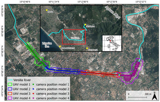
Figure 1.
Study area showing the extent of the four DEMs derived from UAV surveys.
From the Apuan Alps, many steep streams characterized by a typical torrential regime (namely general low flow rate and high flow rate following heavy rainfall) flow down towards the Ligurian Sea, crossing the Versilia plain. The Versilia River (22 km long) is one of the most important of the area, with a basin extension of 160 km2. Although this area has always experienced floods and disasters sometimes associated with life losses, human activities have extensively increased. Over the centuries, these phenomena have induced many hydraulic works aimed at contrasting the risks of flooding in the area, but the interventions have sometimes been ineffective [21,22]. After the 19 June, 1996, hydrogeological disaster, which resulted in 13 deaths and in the damage worth hundreds of millions of euros [23], a deep hydraulic re-arrangement of the Versilia River was made to defend the area from flood risk. The important 1996 event was the last one to hit the study area [21], and for this reason, it is difficult to judge whether the hydraulic works actually managed to protect the area.
3. DEMs
3.1. LiDAR DEM
A LiDAR DEM created by the Italian Ministry of the Environment and Protection of Land and Sea (Ministero dell’Ambiente e della Tutela del Territorio e del Mare, MATTM) is freely available (http://www.pcn.minambiente.it/mattm/). It was acquired using the laser-scan systems Airborne Laser Terrain Mapping (ALTM) Gemini, ALTM 3100EA, and Pegasus of the Optech Incorporated (Vaughan, Ontario, Canada) from 25 January 2008 to 29 October 2010, in near infrared (1064 nm). According to the metadata, the aerial shots were analyzed by means of statistical techniques (Terra Match module of software TerraScan of Terrasolid Ltd., Helsinki, Finland) and were classified for the creation of the models. MATTM states a positional accuracy of 30 cm [24]. The Italian Ministry releases a DTM, a DSM obtained from the first peak of the sensor, and a DSM obtained from the last peak of the sensor at a 1-m resolution. In the present study, we use both the DTM and the DSM obtained from the first peak of the sensor (hereafter simply referred to as DSM).
3.2. DEM from the Structure from Motion Photogrammetry Method
The structure from motion photogrammetry method is a photogrammetric methodology that allows one to reconstruct 3D models, starting from a series of photos with the same elements obtained from different points of view. The use of a UAV equipped with a consumer-grade camera and the use of SfM made it possible to collect low-cost, high spatial resolution, three-dimensional topographic data [25,26,27]. The UAV that we employed was a DJI F550 supplied by the Istituto Nazionale di Geofisica e Vulcanologia of Pisa, Italy. It is a hexacopter with load capacity of 2.4 kg and flight autonomy of 20 min. The camera was a Sony NEX-5T of 111 × 59 × 38 mm in size and a mass of 0.39 kg, able to take pictures of 4912 × 3264 pixels. The E 16-50-mm zoom lens had a 24–75 mm focal length, an 83–32° field of view, and a minimum aperture of f/22–f/36. Further details about the UAV system used in this work are described in Nannipieri et al. [28].
The overflight was planned and managed automatically by Ground Station v4.0.11 software (Dà-Jiāng Innovations Science and Technology Co. Ltd. (DJI), Shenzhen – China) so as to ensure flight altitude, craft velocity, and imaging frequency capable of providing a sufficient overlap between images can be obtained to allow for SfM reconstruction. All acquisitions were achieved at a fixed zoom of 16 mm, and the images were taken at an oblique angle of 24° from the vertical. As a result, pixel viewing angles ranged from 0° (for the pixel immediately below the drone) to 48° (for the furthest pixels along the flight line). The total angular field of view in the cross direction was 83°. This ensured that each pixel was viewed at sufficiently diverse angles so as to reduce overall geometric errors when compared with a vertical view [29].
The SfM allows one to reconstruct automatically and concurrently the 3D model of a portion of territory and the relative position and orientation of the acquisition system. However, subsequent georeferencing of the 3D model requires the identification of the ground points of already known coordinates. Here, we used R10 Trimble real-time kinematic (RTK) Differential GPS(DGPS).
We processed the photos and the GCPs using the Photoscan software (Agisoft LLC, St. Petersburg, Russia), which implements SfM and multi-view stereo matching algorithms. Agisoft Photoscan Professional is one of the most commonly used commercial software products for research in geosciences and archaeology.
The first stage in the standard workflow with Photoscan is to load a set of images and to assess their quality. Photoscan finds matching points between overlapping images, it estimates the position of the camera for each photo, and builds a sparse point cloud model. If a precalibrated camera is not used, the camera correction parameters are also calculated. Then, when available, GCPs are identified in the images and their coordinates are inserted. According to the Photoscan tutorial, to generate an accurately georeferenced orthomosaic, at least 10–15 GCPs should be distributed evenly within the area of interest. The GCPs are generally used as control points to optimize camera positions and orientation data allowing for better model referencing results. It is also possible to use some of these GCPs, not as control points, but as checkpoints so as to assess the absolute accuracy of the 3D model. Since the GCP coordinates are known with good precision, camera alignment should be optimized to achieve higher accuracy in calculating external and internal camera parameters and to correct possible distortions [30].
The next step is the creation of a dense point cloud based on the estimated positions and parameters for each camera. Finally, a DEM and an orthomosaic are computed with pixel sizes that depend on the average ground sampling resolution of the original images.
4. Flooding Model
For the simulation of the channel flows, we used the FLO-2D Basic model, freely available in its basic version [18]. It consists of a quasi-2D hydrological–hydraulic dynamic flow model simulating channel flow, and unconfined overland flow over complex topography. The two-dimensional representation of the motion equation is defined as an almost two-dimensional model using a system of square cells. The motion equation is solved by calculating the average velocity across the cell boundaries in the eight potential flow directions (four hinges and four diagonals). Each speed calculation is one-dimensional and is solved independently by the other seven directions [30]. The main physical processes simulated by the FLO-2D Basic model are the motion of the superficial flow on the floodplain, channeled flow, connection between floodplain and channels, rain, superficial infiltration processes, and hydraulic structures [30]. The channel flow is simulated in one dimension with the channel geometry represented by natural, rectangular, or trapezoidal cross-sections.
Our aim was to simulate the river flow in the computational domain, shown in Figure 2, for a total river reach length of 7.5 km and a total elevation drop of 27 m. In this work, we were not interested in studying plain flooding but only the occurrence of flooding and the outflow points; therefore, we chose a buffer region of 100 m around the center of the riverbed as the computational domain, and a cell size of 15 m. This choice also allowed for the calculation to be sped up, thus reducing the running time. We modeled the river flow using 83 natural sections derived from the described DEMs and positioned along the studied stretch of the river, as shown in Figure 2. The section lengths ranged between 15 and 40 m. The sections were represented by 100 or 300 points, according to the resolution of the DEMs that were used: 100 points were sufficient to describe the channel geometry at the lower resolution of the LiDAR DEM, while for the higher resolution of SfM DEM, 300 points (maximum value allowed by the software) were needed. The area covered by the 41 red sections in Figure 2 was the region where we tested the influence of topography on the channel flow. These sections could be either the simplified sections, or the sections sampled on LiDAR DTM/DSM, or sampled on SfM DEM, according to the tested topography. Black sections were sampled on the LiDAR DTM and represented a buffer region to minimize boundary effects on the studied area.
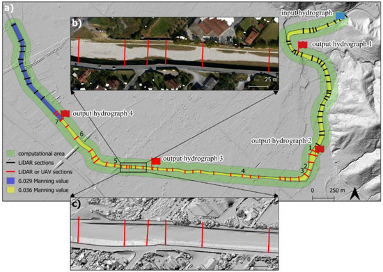
Figure 2.
FLO-2D model set up. (a) Computational domain with FLO-2D model input sections (in green): sections extrapolated from LiDAR (in black) and sections extrapolated from LiDAR or UAV models as described in the text (in red). The blue flag shows the location of input hydrographs, while red flags show locations of output hydrographs. The yellow and blue polygons represent the Manning value of 0.036 and 0.029 used in the models. Numbers indicate the location of the cross-section profiles in Figure 7. The hill-shaded background is from the LiDAR DTM. (b) Ortomosaic zoom-in of a river segment, and location of the FLO-2D input sections (in red). (c) Hill-shaded zoom of the UAV DSM with the location of the FLO-2D input sections (in red).
Since each cell of the computational domain lying on the left bank of the river (441 cells) needed to be associated with one profile, the missing sections were linearly interpolated from the sections derived from DEMs. The average spacing between the DEM-derived sections complied with the indications of the FLO-2D reference manual [30], which suggests a spacing between input sections of 5–10 grid elements. The sections were appropriately positioned in correspondence with topographic variations in order to obtain a gradual transition between wide and narrow reaches, and to avoid the presence of bridges, vegetation, power wires, etc.
Figure 2 also shows the values of channel Manning’s n coefficient following an indication from the Basin Authority of the Po River [31]: the 0.036 value was used where the channel ran on alluvial deposits with pebbly beds and on more irregular bank slopes covered with shrub vegetation. Elsewhere, the 0.029 value was used where the channel ran on alluvial deposits with sandy beds and on more regular bank slopes covered with grass.
Different simulations were set up by varying channel inflow hydrographs at the inflow point of Figure 1. A first group of simulations was performed fixing the limiting channel’s Froude number to 0.6, as suggested by the software manual. We then also investigated the effects on the maximum flow rate of variation of both the Manning and Froude numbers.
5. Results
5.1. DEMs from Structure from Motion
We used 2651 photos and 168 GCPs to construct the 3D model. The study area, 0.59 km2 wide, was divided into four sectors. For each sector, we conducted a distinct flight survey and derived a distinct model (Figure 1). Overall, the flight height was about 50 m above ground level, and photos were taken with a ground pixel resolution of ≈ 1.5 cm. Table 1 shows the main parameters of the four flights. In relation to the above described acquisition geometry, for a flight altitude of 50 m above ground level (AGL), the image area was trapezoidal, with a 56 m width, 74 m length for its short edge, and 112 m for its long edge, resulting in an imaged area of 5100 m2. Considering that the total number of photos was 2651 and the total coverage area was 0.59 km2, each point of the surveyed area was imaged on average 23 times.

Table 1.
Main parameters of the four UAV surveys.
5.1.1. Error Analysis of Photoscan Model 1
Model 1 was used to validate and assess the accuracy of the 3D SfM model and its derived DSM. For this reason, we acquired a large number of GCPs during two different field surveys. During the UAV survey, 59 well-visible targets (Figure 3) were positioned on the ground and their coordinates were acquired using the RTK DGPS to obtain a considerable number of markers for the Photoscan model. The second set of GCPs (194 points) was acquired shortly after the UAV survey and used only to evaluate the RMSE of the derived SfM DSM (Figure 4).
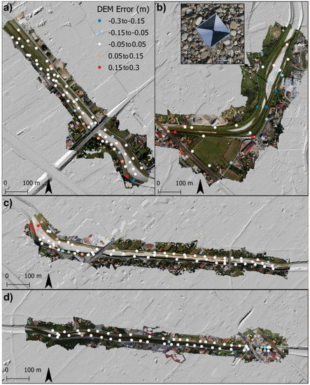
Figure 3.
Spatial distribution of the GCPs used for the model construction (see Table 2 and Table 3). Color coding refers to all the models and shows the vertical differences between DEM and GCP elevation. (a) Model 1; (b) model 4, inset shows an example of the targets captured in the images; (c) model 2; and (d) model 3.
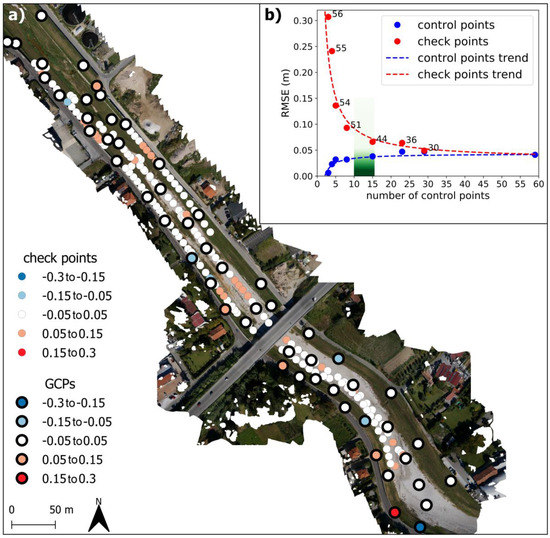
Figure 4.
Model 1 error evaluation. (a) Area distribution of the GPS points used for georeferencing and/or error evaluation. GCPs refer to markers used in the Photoscan model construction (see Table 2 and Table 3). Check points refer to the independent set of points to check DEM accuracy. (b) Control points RMSE (blue dots) and check points RMSE (red dots) of Photoscan models were built as a function of the number of control points used. The green strip shows the value range of the number of GCPs suggested by the Photoscan Tutorial for accurate model georeferencing. See the text for details.
From the 59 markers available, we computed 30 different 3D test models by varying the number and distribution of the control points in order to assess their influence on the model accuracy. Photoscan yields the residual in x, y, and z discrepancies (hereafter control pts RMSE) between the ground coordinates of the control points and their calculated position in the 3D model after the minimization procedure used to optimize camera positions and orientation data (see the RMSE control points in Figure 4b). Since minimization is performed on these points, the control pts RMSE is a function that increases with the number of control points (Figure 4b) and is expected to converge to the accuracy of the model for a sufficiently high number of control points.
For each test model, the markers not used as control points were used as check points. For the check points, Photoscan computes x, y, and z RMSE (hereafter check pts RMSE) between their ground coordinates and their calculated position in the 3D model. This is the common way to assess the real accuracy of models, bearing in mind that we need a statistically significant number of check points and that we have an intrinsic GPS measurement error.
Figure 4b shows the control pts total RMSE and check pts total RMSE as functions of the number of points when the points were evenly distributed in the area. For example, in the case of n = 3 (minimum number of control points necessary to georeference the model), the control pts total RMSE was very small (around 6 mm) and the model was overall very inaccurate, having a check pts total RMSE of 30 cm, calculated using a significant number of points (56). By increasing the number of control points, even if the control pts total RMSE increased, the accuracy of the model also increased, as shown by the rapid drop in the check pts total RMSE. When we selected 29 control points and 30 check points, the control and check total RMSEs were very similar (4.7 cm and 4.9 cm, respectively). When we used all the markers as control points, the control pts total RMSE was 4.1 cm and the control pts z RMSE was 2.8 cm (Table 2). Also the distribution of the control points had a high impact on model accuracy: control points evenly distributed in the area allow one to minimize the so-called bowl effect [29]. Instead, if the control points are concentrated in a small region of the model, the control pts total RMSE decreased slightly while the check pts total RMSE gets much worse, i.e., the model had a much lower overall accuracy since the bowl effect was no longer reduced by the control points. For example, if we used eight control points concentrated within a third of the area of the surveyed region, the check pts total RMSE was around 30 cm, compared to the value of 9.3 cm in the case of eight control points evenly distributed in the whole region.
Table 2.
Root-mean-square discrepancies between the coordinates of the GPS control points and their calculated position in the Photoscan models.
The acquisition camera was calibrated by the lens tool function of PhotoScan, which uses a standard black-and-white chessboard grid to calculate the focal length and distortion properties of the lens so as to provide a lens-distortion correction. Since each point was reconstructed from 23 pictures on average, there were practically no differences between the test models done with or without precalibration of the camera.
Photoscan allows one to choose the quality of calculation of the dense cloud of points. The higher quality and the most computationally expensive option are “ultrahigh”; however, we did not use this function, which is generally recommended for models with very sharp images taken at close range and not for aerial images. We built dense clouds both with “high” and “medium” quality options to investigate the differences and the influence on our hydraulic modeling. The option “high” implies that the input images are downscaled by a factor of 4 before processing and by a further factor 4 for the option “medium.” Therefore, for example, the dense cloud for the model of region 1 derived with the “medium” option had 42,700,000 points, while the one derived with the “high” option has 170,000,000 points.
5.1.2. Error Analysis of Model 1 DEM
The PhotoScan software allowed us to directly build a DEM as well as a stitched and orthorectified aerial image of the entire area. The recommended pixel size of the orthomosaic was 1.43 cm, which was the ground pixel resolution of the input photos. The recommended resolution for the DEM depended on the quality setting used for the generation of the dense point cloud: the “high” quality reconstruction yielded a DEM with a cell size of 2.86 cm for a total of 25,000 × 28,000 pixels, and the “medium” quality reconstruction yielded a DEM with cell size of 5.72 cm for a total of 12,500 × 14,000 pixels. As the vertical error was the only measurable or perceivable error in the DEMs [32], we compared the DEM error with the vertical errors of the Photoscan 3d model. The z RMSE of the Photoscan 3D model was 2.8 cm (Table 2) when all the markers were used as control points. To assess the z accuracy, we needed to use some of the markers as check points. The model with 29 control points and 30 check points gave a vertical accuracy (check z RMSE) of 3.9 cm. This compared very well with the DEM’s vertical RMSE calculated using the 48 markers inside the channel of 4.2 cm (Table 3). Since the PhotoScan model was built upon minimizing the RMS deviation from these markers, they were not an appropriate set of points to check the accuracy of the DEM. For this reason, we collected an independent set of 194 RTK DGPS points inside the channel, obtaining an RMSE for the DEMs (for both the 2.86 cm and 5.72 cm cell sizes) of 4.0 cm (Figure 4). For the evaluation of the DEM errors, we considered the internal channel area (Table 3) and the top of banks/wall separately. The points on the walls had a much higher error since walls were generally very thin (down to 25 cm), and for this reason they were not well represented on the DEM (Figure 5).
Table 3.
RMSE of the source and resampled UAV DEMs.
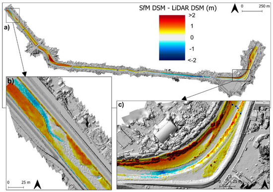
Figure 5.
Difference between SfM DSM and LiDAR DSM inside the channel. a) Studied area; b and c) magnified areas corresponding to the black boxes in frame a.
5.1.3. Error Analysis of Merged DEMs
The vertical and total RMSEs of the four Photoscan models were similar to the values of model 1 (Table 2); in particular, the vertical RMSE ranged between 2.2 and 2.8 cm (with an average RMSE of 2.5 cm) and the total RMSE ranged between 3.3 and 5.6 cm (with an average RMSE of 4.0 cm).
To validate the total RMSE for models 2, 3, and 4, we calculated the check total RMSEs considering half of the markers as check points. These were 3.7, 3.7, and 7.0 cm, respectively, which were only slightly worse than the total control RMSEs of 3.3, 3.8, and 5.6 cm, respectively (Table 2, where all the points were considered as control points), in agreement with the general trend of the plot in Figure 4b.
The four DEMs of the regions of Figure 1 were then built from Photoscan dense clouds obtained with the “medium” quality option. For better management, we merged the complete dataset in a single DEM with a grid step of 10 cm (hereafter SfM DSM) for 34,150 × 14,400 pixels. The DEMs of the first three regions, where the thin walls were located, were exported with the original cell size (around 5 cm), and then resampled to 10 cm, while the fourth DEM was exported from Photoscan directly with the 10 cm cell size. For the first three regions, we also built a dense cloud with the “high” quality option, obtaining three DEMs with cell sizes around 2.8 cm. Again, we resampled these DEMs and merged them with the fourth DEM, which produced another 10 cm cell size model (hereafter SfM DSM+).
The SfM DSM and SfM DSM+ errors were evaluated using 228 points acquired during the UAV survey, which included 168 markers. The RMSE was 4.8 and 4.7 cm, respectively for the inside, and 12.5 and 9.8 cm, respectively, for the top of the banks/wall. The merging operation made it possible to eliminate overlapping areas of the DEMs, where errors were high (Figure 3). Also, for this reason, the RMSEs of the SfM DSMs were lower than those of the source DEMs despite the greater cell size.
5.2. Topographic Data and Flow Modeling
5.2.1. Morphological River Channel Changes
The difference between the SfM DSM and the LiDAR DSM inside the channel shows the morphological changes occurred between the SfM acquisition (2018) and the LiDAR acquisition (2008–2010, Figure 5). Considering that the channel was not completely empty during the LiDAR acquisition, while it was dry during the UAV survey, the reddish areas were certainly deposition zones up to 200 cm accumulated in 8–10 years (without considering the vegetated areas). Bluish hues represent either erosion areas or wet areas during the LiDAR survey. The differences between the channel morphology from LiDAR DSM and from SfM DSM are clearly visible in the channel cross section in Figure 6e and Figure 7.
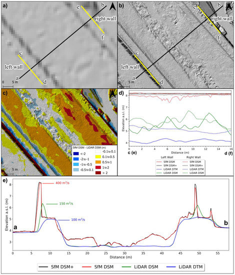
Figure 6.
DEM analysis of relevant hydraulic features. (a,b) Hillshaded maps of the 1-m LiDAR DTM and SfM DSM, respectively. (c) Difference between SfM DSM and LiDAR DSM. (d) Longitudinal profiles along the embankment walls (yellow lines in frames a and b). (e) Profiles of the river cross section (black lines in frame a and b). Flow rate values show the maximum flow rate for the different DEMs according to FLO-2D simulations.
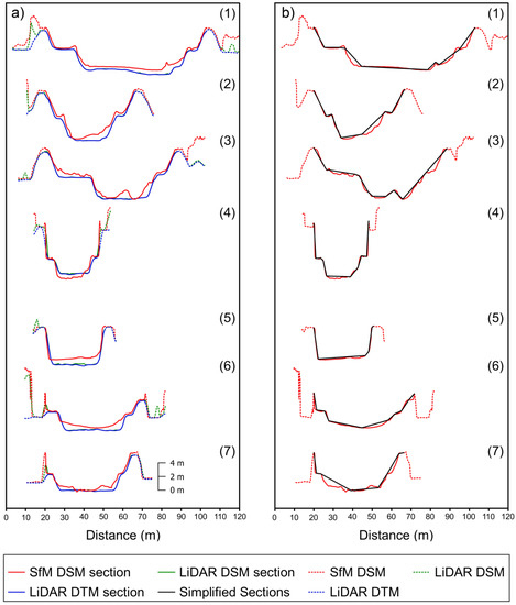
Figure 7.
Comparison of the cross-section profiles derived from different topographic data. See Figure 2 for the locations of the cross-sections along the channel. (a) Profiles derived from SfM DSM, LiDAR DSM and DTM. (b) Profiles derived from SfM DSM and Simplified Sections.
5.2.2. Hydraulic Features and Grid Resolution
Hydraulic simulations heavily depend on the relevant features (e.g., channel bottom shape and depth, bank shape and height), which are well-solved in the DEMs available. Figure 6e shows a typical section of this river, where thin high walls are superimposed to the river banks. In the LiDAR DTM profile (blue line in Figure 6d,e), the river embankment walls were absent; the filtering processing used for DTM realization was calibrated to remove anthropic features such as buildings and walls. In the LiDAR DSM profile (green line in Figure 6d,e), the walls were only partially represented because of the low resolution. Indeed, a 1-m cell size DEM was unable to resolve a 40 cm thick wall, as in this case (Figure 6a). The SfM DSM (originally a cell size around 5 cm and resampled to 10 cm, red line in Figure 6d,e) reproduced the two embankment walls, but the right wall was up to 70 cm lower than the left one. The SfM DSM+ (originally a 2.8 cm cell size DEM resampled to 10 cm, black line in Figure 6d,e) reproduced the two embankment walls better than the other DEMs.
The SfM DSM errors were comparable with the GPS acquisition error, hence a very dense GPS section would be practically identical to the SfM DSM section. For this reason, we added another dataset of simplified sections by extracting the points at the main breaks in the slope directly from the SfM DSM in order to mimic a GPS acquisition with a minimal set of points (simplified sections in Figure 7).
5.2.3. Hydraulic Model Comparison
We set a step function with increments of 50 m3/s up to a maximum input rate of 600 m3/s as the model inflow hydrograph (Figure 2). This choice allowed us to check stationary conditions at different flow rates. The flow rates of the different models were compared at four points along the simulated channel reach (Figure 2): the first point was at 1 km from the inflow point, and was the only one outside the area covered by the SfM DEMs; the second, third, and fourth points were at the beginning, middle, and end of the area covered by SfM DEMs, respectively (Figure 2). In this way, we could monitor the simulated flow in the river according to the different topographic data (Figure 8 and Figure 9).
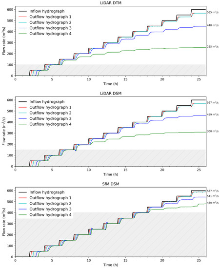
Figure 8.
Flow rates computed using FLO-2D at four different sections (see Figure 2) for an input flow step function with 50 m3/s increments (maximum input rate 600 m3/s) in the simulations based on LiDAR DTM, LiDAR DSM, and SfM DSM. The shaded area highlights the flow rate range without flooding.
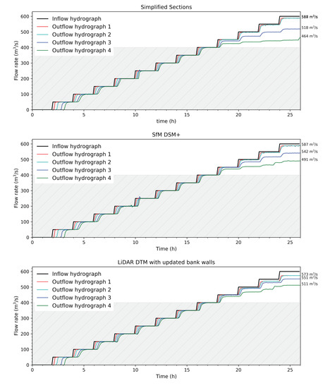
Figure 9.
Flow rates computed using FLO-2D at four different points (see Figure 2) for an input flow step function with 50 m3/s increments (maximum input rate 600 m3/s) in the simulations based on simplified sections extracted from the SfM DSM, SfM DSM+, and LiDAR DTM with bank walls updated using the SfM DSM. The shaded area highlights the flow rate range without flooding.
We tested the influence on our simulations of the limiting channel Froude number 0.6 by running the models, also with a limiting value of 1.2. Comparison of the output shows a maximum variation of the flow rate within 4%.
We also investigated the effect of changes in the Manning value. We lowered the 0.036 value to 0.029, which, according to the instructions of the Basin Authority of the Po River [31], corresponded to a change in the channel roughness class from regular river beds having irregular slopes with shrubs to sandy river beds having regular slopes with grass coverage. The results show an increase in the maximum flow rates of up to 15% for LiDAR DTM and 8% for SfM DSM. On the other hand, by increasing the Manning value to 0.040, we obtained a decrease in the maximum flow rates up to 20% for LiDAR DTM and up to 12% for SfM DSM.
6. Discussion
In fluvial hydraulic modeling, the terrain details play a major role in the potential achievement of reliable results. The best DEM available for the area is the LiDAR DEM by MATTM, with a 1-m resolution and dating back to 2008–2010. The use of LiDAR data as a topographic computational base for hydraulic modeling implies the choice between LiDAR DTM and LiDAR DSM. DTM lacks all the anthropic features that often interrupt the river course and that are instead present in DSM (bridges, power lines, vegetation, etc.). Considering that FLO-2D computes the channel flow in one dimension using only sparse input cross-section profiles as topographic data, the presence of obstacles along the river channel is easily solved via a targeted choice of the section position. A comparison between the simulations using LiDAR DTM and DSM shows that the maximum flow rate with no outflow was 100 m3/s and 150 m3/s, respectively (Figure 8). As already mentioned, the difference was due to the filtering processing method used for DTM realization, which removed all the embankment walls (e.g., Figure 6e and Figure 7). This reach of the river had an estimated maximum flow rate of at least 400 m3/s [33,34], much higher than the result of the simulations based on the LiDAR data.
Such flow rate discrepancies are one order of magnitude greater than that introduced by one shift in the roughness class for the Manning parameters of the channel.
In an attempt to achieve a more realistic simulation output, we improved the input topographic data with three different actions: (1) adding the embankment walls to the LiDAR data with a targeted DGPS survey, (2) directly acquiring the cross-section profiles with a targeted DGPS survey, and (3) realizing a very high resolution topography using the structure from motion techniques from images acquired using UAV. We opted for the last solution because a very-high-resolution DEM would also allow us to indirectly evaluate the pros and cons of options 1 and 2. Option 1 requires the shortest acquisition time in the field, but it delivers very poor results since the riverbed has undergone great changes over the last ten years (Figure 5, Figure 6 and Figure 7). Option 2 would require a DGPS survey to achieve, with a high density of points, as seen in the red sections shown in Figure 2. This, however, would yield simulation results very similar to those of the SfM DSMs since the SfM DSM error is of the same order of precision as the GPS acquisition error. Such a GPS campaign would take a comparable, if not longer time, than that necessary for UAV surveys and subsequent post-processing. The survey time could be reduced by acquiring only the main break-in slope points; the outcomes of this operation are indirectly evaluated in Figure 9 by deriving the simplified sections from SfM DSM.
When planning the aerial surveys, we decided to investigate the influence of the number of GCPs on the resolution and error in the final DEMs in order to improve future acquisitions. Thanks to the high number of GCPs obtained, we assessed the Photoscan models and DEM errors so as to obtain a total RMSE between the GCPs and their calculated position in the 3D model of 4.0 cm. Using some of the GCPs as check points, we evaluated the accuracy of Photoscan model 1 to be less than 4.9 cm (Figure 4b). Following the recommendation of Photoscan, which uses 10–15 GCPs uniformly distributed to reduce the bowl effect [29], the corresponding errors would have been in the 7–9 cm range, which are totally acceptable for our aim; furthermore, by acquiring 10–15 points instead of 59, the survey duration would have been reduced by 50%.
The independent set of GPS collected in a successive campaign allowed us to assess the accuracy of SfM DSM, obtaining a total RMSE of 4.0 cm. With a flight height of 50 m, we obtained a ratio of error against the flying height of 80 cm/km, comparable to 66.7–100 cm/km measured by Vallet et al. [35] and 50–80 cm/km by Harwin et al. [36].
The maximum flow rate using the SfM DSMs as a topographic base was around 400 m3/s (Figure 8), in agreement with the estimated maximum flow rate of the river [33,34]. This flow rate was 2–3 times the one estimated using LiDAR data. In terms of surface detail, this result is well explained, for example, in the profile comparison of Figure 6e. The profile of LiDAR DTM was able to capture only the larger earth embankments, but it completely missed the walls; consequently, the maximum flow depth was around 2.5 m, and the maximum flow rate was only 100 m3/s. The LiDAR DSM captured a portion of the embankment walls, allowing a maximum flow depth of 4 m and reaching a maximum flow rate of 150 m3/s. The much higher maximum flow rate of the simulations based on the SfM DSMs was due to their good capability of reconstructing even the thinner embankment walls with a maximum flow depth of 5.5 m.
The SfM DSM and SfM DSM+ simulation results were similar but not identical: although both models had the same maximum flow rate, they behaved differently for input flow rates over 400 m3/s. These disparities can be attributed to small morphological diversities between the two DSMs, as shown in Figure 6e, where the right embankment wall was ≈ 20 cm higher on the SfM DSM+. A comparison of the profiles along the top of the walls showed not only that the LiDAR DEMs greatly underestimated the height of the walls, but also that there were some discrepancies between SfM DSM and SfM DSM+ (Figure 6d). In particular, the right wall was better represented in SfM DSM+, where the wall had a constant height, while the height of the top of the wall in the SfM DSM was lower and irregular. This implies that the source DEM of the SfM DSM+ (cell size ≈ 2.8 cm) had a better resolution than the source DEM of the SfM DSM (cell size ≈ 5 cm), and that the latter instead had a resolution that was worse than 10 cm. While the former implication was expected, the latter implication was not. For this reason, it will be necessary to build the Photoscan model with a better option and to resample the grid to the appropriate cell size at a later time.
The plot of the flow rate of the simulation based on the simplified sections in Figure 9 gave results similar to the simulations based on the SfM DSMs. This means that the overall profile could be greatly simplified, as long as the main break-in slope points and the correct height information of the walls were present (Figure 7). This suggests that a speedy DGPS survey acquiring only the main break-in slope points could be sufficient for fluvial hydraulic modeling. The greatest limit of this approach is that, once acquired, the sections were fixed and could not be moved to solve any problems arising during the modeling phase. In the case of LIDAR DTM with updated bank walls (the best representation of the channel geometry of 8–10 years ago), the maximum flow rate was again around 400 m3/s (Figure 9).
The inflow hydrograph was a step function with increments of 50 m3/s up to a maximum input rate of 600 m3/s. This function enabled us to check the stationary conditions at different flow rates (Figure 8 and Figure 9). Figure 10 shows the relation between flow rates and flow height in one section for different topographic data. In frame (c), the dots represent flow height values calculated using FLO-2D for the above mentioned steady flow rates, and the dashed lines are the rating curves according to the flow rates Q = AV, where A is the wet area and V is the cross-sectional average velocity, derived from the Manning formula [37]:
where n is the Manning number, Rh is the hydraulic radius, and S is the channel bed slope. Different values of S were chosen to fit the data points, case by case.
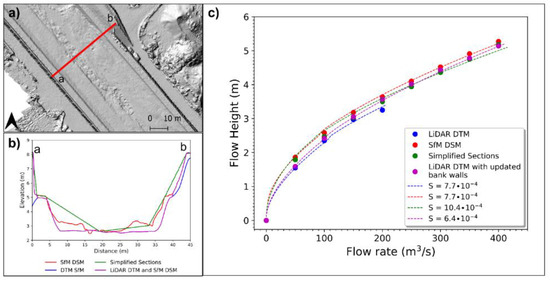
Figure 10.
The relation between flow rates and flow height for different topographic data: (a) position of the section, (b) section profiles, and (c) flow height vs. flow rates plot where dots are calculated using FLO-2D and dashed lines are the rating curves calculated using the Manning Formula (Equation (1)).
Overall, there was a good fit between the flow rates derived from the Manning formula and the ones computed using FLO-2D, although the flow rates derived from the Manning formula depend only on the shape of the considered section; instead, the flow rates calculated using FLO-2D at any section also depend on the shapes of the nearby sections. In the flow height versus flow rate plot (Figure 10c), the rating curves SfM DSM and LiDAR DTM with updated bank walls were very similar in terms of shape and fitting slope values (0.00078 vs. 0.00075). They differ for an offset in the flow height up to 40 cm. SfM DSM had an irregular bottom profile compared to LiDAR DTM, which had a much more regular flat channel bottom. The flow height was calculated from the minimum elevation, which introduced the height gap in the plot.
The rating curve derived from the simplified sections had a different trend and different slope compared to the two previous cases. This was due to the rough simplification of the profile across the river. The profile (7) of Figure 7, identical to that of Figure 10, was the worst approximation of the real profile. Nevertheless, the corresponding values in Figure 10c agreed with those derived from the other topographic data. In the case of LiDAR DTM, as the flow rate approached the maximum value of 200 m3/s, the rating curve differed more and more from the LIDAR DTM curve with updated bank walls.
In Figure 10b, the comparison between SfM DSM and LiDAR DSM gave the morphological variation of the river bed that had occurred in the last 8–10 years, including erosion and deposition areas. In this section, there was a net deposition of up to 1 m. According to Figure 10c, if the channel was affected by a 1-m deposit, it should have a flow rate reduction of 140 m3/s. In the study, area the deposition was limited to only a few areas with small thickness (Figure 5). If it had an influence on the maximum flow rate without flooding (shaded area in Figure 9), this effect was less than 50 m3/s, since it was not visible in Figure 9, because of the chosen step function of the inflow hydrograph.
Given the good fit between the flow rates derived from the Manning formula and the ones computed using FLO-2D, a quantitative study of the influence of topography resolution on the maximum flow rate for different channel geometries could be performed using Q = AV, where A is the wet area and V is given by the Manning formula (Equation (1)). The 10 cm cell size SfM DSM was resampled to increasing cell sizes from 30 to 290 cm, with steps of 20 cm. The new DEMs were derived by averaging the 10 cm cells inside each new cell, for example, each cell of the 290 cm DEM was obtained by averaging the 29 × 29 10 cm cells inside it.
By increasing the cell size, i.e., decreasing the resolution, the maximum flow rate generally decreased in all cases. In section 3 of Figure 11, the embankment walls had dimensions greater than the maximum resampled cell size, the profiles do not change significantly if the cell sizes are varied, and the maximum flow rate decreased very slowly at increasing cell size, and showed a perceptible decrease only after 250 cm.
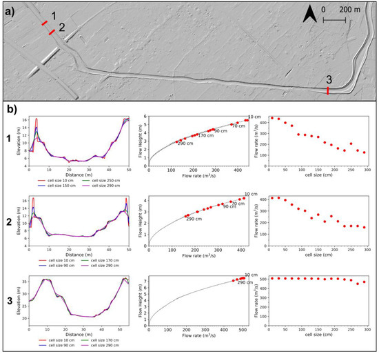
Figure 11.
Effect of topography resolution on the maximum flow rate for three selected sections. (a) Hill-shaded map of a reach of the Versilia River with the location of the sections. (b) Plots of topographic profiles, maximum flow rate vs. maximum flow height, as function of the topography resolution and maximum flow rate vs. cell size.
On the other hand, in sections 1 and 2, the effect of decreasing the cell size was more marked: a 1-m cell size corresponded to a maximum flow rate of 280–320 m3/s, a 2 m cell size corresponded to a maximum flow rate of 200–230 m3/s, and a 3-m cell size corresponded to a maximum flow rate of 100–150 m3/s. Section 1 profiles displayed embankment walls with very different thicknesses: the thickest one, well-reconstructed at all investigated cell sizes, did not affect the flow rate; the thinner one (about 50 cm thick on the top) was solved well only at the resolution of 10–30 cm. From cell sizes of 30 cm to 90 cm, the maximum flow rate dropped from over 400 m3/s to under 300 m3/s. In terms of the maximum flow rate, the values of 100 to 150 m3/s deriving from the simulation with LiDAR were consistent with a cell size of about 3 m for sections 1 and 2 of Figure 11. This was consistent with the fact that this LiDAR DEM, despite its 1-m cell size, had a much worse resolution.
7. Conclusions
In this study, we have focused on the effects of topographic resolution and accuracy on channel flow rates. In our case, they were much more relevant than, for example, channel roughness, which is considered an important source of uncertainty in hydraulic simulations [11,38].
The best freely available DEM for the study area is the LiDAR DEM by MATTM, dating back to 2008–2010. However, despite its good 1-m nominal resolution, it is not suitable for FLO-2D simulations because these topographic data cannot represent geometries smaller than 1 m. This means, for example, that some of the embankment walls of the channel were missed out (e.g., Figure 6e). The absence or misrepresentation of these structures caused the greatest errors in hydraulic simulations, and produces significant deviations from reality (Figure 8). Simulations derived from both LiDAR DTM and DSM gave a maximum flow rate with no outflow of 100 and 150 m3/s, respectively, whereas the expected value was around 400 m3/s [33,34]. This problem can only be solved using topographic data able to represent all the embankment structures. For example, we could add the missing structures, reconstructed using GPS surveys, to the LiDAR DEM. When a low-resolution DEM (like LiDAR DEM) is available, this approach is the least expensive in terms of resources. However, in our case, the simulation results refer to a depositional situation of the river bed dating back to 2008–2010.
Adequate topographic data can also be obtained by acquiring the necessary river cross-sections with a dedicated GPS survey. Both time and resources, comparable to those necessary to perform a UAV survey and to apply SfM for an updated high-resolution DEM, are needed to update a pre-existing DEM or to collect a number of cross-sections. Furthermore, collecting only the necessary river cross-sections has some limitations compared to a full UAV survey, which is able to deliver a high resolution SfM DEM. Once acquired, the sections are fixed and cannot be moved to solve any problems arising during the modeling phase. In order to have a detailed shape of the section like the one obtained using SfM, many points are required for each cross-section, consequently considerably prolonging the campaign duration; GPS cross-sections give 1D data, while UAV-SfM techniques deliver 2D data that can also be used to track morphological variations of the riverbed.
Therefore, we reconstructed a high-resolution 3D model using Agisoft Photoscan Professional from 2651 photos and 168 GCPs. The root-mean-square discrepancy between the coordinates of the GPS ground control points and their calculated position in the Photoscan model was 4.0 cm. The error on the derived 10-cm DEM was independently assessed using a new set of 194 GPS points inside the channel, which obtained an RMSE of 4.0 cm. This study highlights some considerations in the use of Photoscan for the realization of DEMs as input topographic data for hydraulic simulations. The cell size suggested for the DEM exported by Photoscan is not the resolution of the DEM itself; therefore, the choice of the calculation quality of the dense cloud is very important. Setting the quality to “high” or to “medium” influenced the way in which the very narrow embankment walls were represented in the DEM. Indeed, SfM DSM RMSE and SfM DSM+ RMSE for the top of banks/wall was 12.5 and 9.8 cm, respectively. For this reason, it is important to build the Photoscan model with the best possible quality option and to resample the grid to the appropriate, manageable cell size at a later time. The number of GCPs must be evenly distributed to minimize the bowl effect. The Photoscan recommendation of using 10–15 GCPs per model would produce errors in the 7–9 cm range, which would have been acceptable for our aim and would have considerably reduced the duration of the campaign (e.g., model 1, Figure 4).
The availability of the high-resolution 10-cm DEM allowed us to perform channel-flow simulations by testing different topographic data: SfM DSM and SfM DSM+, simplified sections, and LiDAR DTM with updated bank walls (Figure 8 and Figure 9). All these simulations yielded a maximum flow rate around 400 m3/s, in accordance with the expected value. This implies that riverbed changes that have occurred over the last 10 years did not substantially affect the maximum flow rate. Simulations based on the simplified sections shows that overall section profiles can be greatly simplified as long as the main break-in-slope points and the correct height information of the walls are present (Figure 7). This suggests that a speedy DGPS survey acquiring only the main break-in-slope points could be sufficient for fluvial hydraulic modeling but with the great limit that the section positions are fixed and cannot be moved in response to computational demands.
A further analysis of the influence of DEM resolution on the flow rate was performed by degrading the 10-cm SfM-DSM to lower resolutions. We clearly observed that in our case (e.g., section 1, Figure 11), DEMs with a resolution lower than 30 cm already introduced a loss of 10% in the maximum flow rate, with further significant losses up to the minimum investigated resolution. Considering the previous remarks, a UAV-SfM-derived DEM is the best solution for small areas: it is low cost, it has an adequate resolution, and it can be obtained quite rapidly (1–2 km/day). This allows one to accurately monitor the channel morphology variations in time and to keep the hydraulic models updated, thus providing an excellent tool for managing hydraulic and flooding risks.
Author Contributions
Conceptualization, M.L., M.F., I.I., L.N., M.B., R.G.; methodology, M.L., M.F., I.I., L.N.; software, validation, formal analysis, investigation, resources, M.L., M.F., I.I., L.N.; data curation, M.L., M.F.; writing—original draft preparation, M.L., M.F., I.I.; writing—review and editing, M.L., M.F., I.I., L.N., M.B., R.G.; visualization, M.L., M.F., I.I.; supervision, M.F.; project administration and funding acquisition, M.B.
Funding
This work was supported by the Fondazione Cassa di Risparmio di Lucca, within the Project “Clima e eventi alluvionali estremi in Versilia: integrazione di nuove tecniche geoarcheologiche, geomorfologiche, geochimiche e simulazioni numeriche”, 2016-18 (Principal Investigator M. Bini), and by the University of Pisa, within the Project PRA_2018_41 “Georisorse e Ambiente”.
Acknowledgments
The authors are grateful to the reviewers for their helpful and constructive comments and suggestions. They are also grateful to the Ministero dell’Ambiente e della Tutela del Territorio e del Mare for providing the LiDAR data.
Conflicts of Interest
The authors declare no conflict of interest. The funders had no role in the design of the study; in the collection, analyses, or interpretation of data; in the writing of the manuscript, or in the decision to publish the results.
References
- Gao, P.; Hartnett, J.J. Exploring the causes of an extreme flood event in Central New York, NY, USA. Phys. Geogr. 2016, 37, 38–55. [Google Scholar] [CrossRef]
- Jena, P.P.; Chatterjee, C.; Pradhan, G.; Mishra, A. Are recent frequent high floods in Mahanadi basin in eastern India due to increase in extreme rainfalls? J. Hydrol. 2014, 517, 847–862. [Google Scholar] [CrossRef]
- He, H.; Zhou, J.; Yu, Q.; Tian, Y.; Chen, B. Flood frequency and routing processes at a confluence of the middle Yellow River in China. River Res. Appl. 2007, 23, 407–427. [Google Scholar] [CrossRef]
- Huntington, T.G. Evidence for intensification of the global water cycle: Review and synthesis. J. Hydrol. 2006, 319, 83–95. [Google Scholar] [CrossRef]
- Hall, J.; Arheimer, B.; Borga, M.; Brázdil, R.; Claps, P.; Kiss, A.; Kjeldsen, T.R.; Kriaučiūnienė, J.; Kundzewicz, Z.W.; Lang, M.; et al. Understanding flood regime changes in Europe: A state-of-the-art assessment. Hydrol. Earth Syst. Sci. 2014, 18, 2735–2772. [Google Scholar] [CrossRef]
- Merz, B.; Aerts, J.; Arnbjerg-Nielsen, K.; Baldi, M.; Becker, A.; Bichet, A.; Blöschl, G.; Bouwer, L.M.; Brauer, A.; Cioffi, F.; et al. Floods and climate: Emerging perspectives for flood risk assessment and management. Nat. Hazards Earth Syst. Sci. 2014, 14, 1921–1942. [Google Scholar] [CrossRef]
- Grimaldi, S.; Petroselli, A.; Arcangeletti, E.; Nardi, F. Flood mapping in ungauged basins using fully continuous hydrologic-hydraulic modeling. J. Hydrol. 2013, 487, 39–47. [Google Scholar] [CrossRef]
- Arduino, G.; Reggiani, P.; Todini, E. Recent advances in flood forecasting and flood risk assessment. Hydrol. Earth Syst. Sci. 2005, 9, 280–284. [Google Scholar] [CrossRef]
- Bodoque, J.; Guardiola-Albert, C.; Aroca, E.; Galán, M.; Lorena Martínez-Chenoll, M. Flood Damage Analysis: First Floor Elevation Uncertainty Resulting from LiDAR-Derived Digital Surface Models. Remote Sens. 2016, 8, 604. [Google Scholar] [CrossRef]
- Bellos, V.; Tsakiris, G. Comparing Various Methods of Building Representation for 2D Flood Modelling In Built-Up Areas. Water Resour. Manag. 2015, 29, 379–397. [Google Scholar] [CrossRef]
- Dimitriadis, P.; Tegos, A.; Oikonomou, A.; Pagana, V.; Koukouvinos, A.; Mamassis, N.; Koutsoyiannis, D.; Efstratiadis, A. Comparative evaluation of 1D and quasi-2D hydraulic models based on benchmark and real-world applications for uncertainty assessment in flood mapping. J. Hydrol. 2016, 534, 478–492. [Google Scholar] [CrossRef]
- Bates, P.D.; De Roo, A.P.J. A simple raster-based model for flood inundation simulation. J. Hydrol. 2000, 236, 54–77. [Google Scholar] [CrossRef]
- Cook, A.; Merwade, V. Effect of topographic data, geometric configuration and modeling approach on flood inundation mapping. J. Hydrol. 2009, 377, 131–142. [Google Scholar] [CrossRef]
- Meesuk, V.; Vojinovic, Z.; Mynett, A.E.; Abdullah, A.F. Urban flood modelling combining top-view LiDAR data with ground-view SfM observations. Adv. Water Resour. 2015, 75, 105–117. [Google Scholar] [CrossRef]
- Teng, J.; Jakeman, A.J.; Vaze, J.; Croke, B.F.W.; Dutta, D.; Kim, S. Flood inundation modelling: A review of methods, recent advances and uncertainty analysis. Environ. Model. Softw. 2017, 90, 201–216. [Google Scholar] [CrossRef]
- Smith, M.; Carrivick, J.; Hooke, J.; Kirkby, M. Reconstructing flash flood magnitudes using ‘Structure-from-Motion’: A rapid assessment tool. J. Hydrol. 2014, 519, 1914–1927. [Google Scholar] [CrossRef]
- Leitão, J.P.; de Sousa, L.M. Towards the optimal fusion of high-resolution Digital Elevation Models for detailed urban flood assessment. J. Hydrol. 2018, 561, 651–661. [Google Scholar] [CrossRef]
- O’Brien, J.S.; Julien, P.Y.; Fullerton, W.T. Two-Dimensional Water Flood and Mudflow Simulation. J. Hydraul. Eng. J. Hydraul. 1993, 119, 244–261. [Google Scholar] [CrossRef]
- Rapetti, C.; Rapetti, F. L’evento pluviometrico eccezionale del 19 giugno 1996 in Alta Versilia (Toscana) nel quadro delle precipitazioni delle Alpi Apuane. Atti Soc. Sci. Nat. Mem. Ser. A 1996, 103, 143–159. [Google Scholar]
- Rapetti, F.; Vittorini, S. Le precipitazioni in Toscana: Osservazioni sui casi estremi. Rivista Geografica Italiana 1994, 101, 47–76. [Google Scholar]
- Giannecchini, R.; D’Amato Avanzi, G. Historical research as a tool in estimating hydrogeological hazard in a typical small alpine-like area: The example of the Versilia River basin (Apuan Alps, Italy). Phys. Chem. EarthParts A/B/C 2012, 49, 32–43. [Google Scholar] [CrossRef]
- D’Amato Avanzi, G.; Giannecchini, R. Eventi alluvionali e fenomeni franosi nelle Alpi Apuane (Toscana): Primi risultati di un’indagine retrospettiva nel bacino del Fiume Versilia. Rivista Geografica Italiana 2003, 110, 527–559. [Google Scholar]
- D’Amato Avanzi, G.; Giannecchini, R.; Puccinelli, A. The influence of the geological and geomorphological settings on shallow landslides. An example in a temperate climate environment: The June 19, 1996 event in northwestern Tuscany (Italy). Eng. Geol. 2004, 73, 215–228. [Google Scholar]
- MATTM. Ministero Dell’ambiente e Della Tutela del Territorio e del Mare; MATTM: Roma, Italy, 2018.
- Lowe, D.G. Distinctive Image Features from Scale-Invariant Keypoints. Int. J. Comput. Vis. 2004, 60, 91–110. [Google Scholar] [CrossRef]
- Westoby, M.J.; Brasington, J.; Glasser, N.F.; Hambrey, M.J.; Reynolds, J.M. ‘Structure-from-Motion’ photogrammetry: A low-cost, effective tool for geoscience applications. Geomorphology 2012, 179, 300–314. [Google Scholar] [CrossRef]
- Favalli, M.; Fornaciai, A.; Isola, I.; Tarquini, S.; Nannipieri, L. Multiview 3D reconstruction in geosciences. Comput. Geosci. 2012, 44, 168–176. [Google Scholar] [CrossRef]
- Nannipieri, L.; Fornaciai, A.; Favalli, M.; Cipolla, V. Manuale delle operazioni con SAPR e analisi del rischio. In Rapporti Tecnici INGV; INGV: Rome, Italy, 2016. [Google Scholar]
- James, M.R.; Robson, S. Mitigating systematic error in topographic models derived from UAV and ground-based image networks. Earth Surf. Process. Landf. 2014, 39, 1413–1420. [Google Scholar] [CrossRef]
- FLO-2D Software FLO-2D Reference Manual; FLO 2-D Software, Inc. P.O. Box 66: Nutrioso, AZ, USA, 2009.
- Autorità di Bacino del Fiume Po. Direttiva Contenente i Criteri per la Valutazione della Compatibilità Idraulica delle Infrastutture Pubbliche e di Interesse Pubblico All’interno delle Fasce “A” e “B”; Autorità di Bacino del Fiume Po.: Parma, Italy, 2006. [Google Scholar]
- United States Geological Survey. National Mapping Program Technical Instructions: Standards for Digital Elevation Models, U.S. Geological Survery National Mapping Division; United States Geological Survey: Reston, VA, USA. Available online: http://rmmcweb.cr.usgs.gov/public/nmpstds/demstds.html (accessed on 1 March 2019).
- Caredio, F.; D’Amato Avanzi, G.; Puccinelli, A.; Trivellini, M.; Venutelli, M.; Verani, M. La catastrofe idrogeologica del 19/06/1996 in Versilia e Garfagnana (Toscana, Italia): Aspetti geomorfologici e valutazioni idrauliche. In Proceedings of the La Prevenzione dalle Catastrofi Idrogeologiche: Il Contributo della Ricerca Scientifica, Alba, Italy, 5–7 November 1996; Volume 2, pp. 75–88. [Google Scholar]
- Preti, F.; Paris, E. Evento alluvionale del 19 giugno 1996 in Versilia-Garfagnana: Ricostruzione degli idrogrammi di piena. In Proceedings of the Convegno Scientifico in Occasione del Trentennale Dell’alluvione di Firenze: “La difesa dalle alluvioni”, Firenze, Italy, 4–5 November 1996. [Google Scholar]
- Vallet, J.; Panissod, F.; Strecha, C.; Tracol, M. Photogrammetric performance of an ultra light weight swinglet UAV. ISPRS Int. Arch. Photogramm. Remote Sens. Spat. Inf. Sci. 2012, XXXVIII, 253–258. [Google Scholar] [CrossRef]
- Harwin, S.; Lucieer, A. Assessing the accuracy of georeferenced point clouds produced via multi-view stereopsis from Unmanned Aerial Vehicle (UAV) imagery. Remote Sens. 2012, 4, 1573–1599. [Google Scholar] [CrossRef]
- Manning, R. On the flow of water in open channels and pipes, Transactions of the Institution of Civil Engineers of Ireland. Trans. Inst. Civ. Eng. Irel. 1891, 20, 161–207. [Google Scholar]
- Papaioannou, G.; Vasiliades, L.; Loukas, A.; Aronica, G.T. Probabilistic flood inundation mapping at ungauged streams due to roughness coefficient uncertainty in hydraulic modelling. Adv. Geosci. 2017, 44, 23–34. [Google Scholar] [CrossRef]
© 2019 by the authors. Licensee MDPI, Basel, Switzerland. This article is an open access article distributed under the terms and conditions of the Creative Commons Attribution (CC BY) license (http://creativecommons.org/licenses/by/4.0/).