Article

Gaussian Processes for Vegetation Parameter Estimation from Hyperspectral Data with Limited Ground Truth

1
Chester F. Carlson Center for Imaging Science, Rochester Institute of Technology, Rochester, NY 14623, USA
2
Boeing Research and Technology, Huntsville, AL 35824, USA
3
Department of Electrical & Microelectronic Engineering, Rochester Institute of Technology, Rochester, NY 14623, USA
*
Author to whom correspondence should be addressed.
Remote Sens. 2019, 11(13), 1614; https://doi.org/10.3390/rs11131614
Submission received: 12 May 2019 / Revised: 28 June 2019 / Accepted: 30 June 2019 / Published: 8 July 2019

Abstract

:
An important application of airborne- and satellite-based hyperspectral imaging is the mapping of the spatial distribution of vegetation biophysical and biochemical parameters in an environment. Statistical models, such as Gaussian processes, have been very successful for modeling vegetation parameters from captured spectra, however their performance is highly dependent on the amount of available ground truth. This is a problem because it is generally expensive to obtain ground truth information due to difficulties and costs associated with sample collection and analysis. In this paper, we present two Gaussian processes based approaches for improving the accuracy of vegetation parameter retrieval when ground truth is limited. The first is the adoption of covariance functions based on well-established metrics, such as, spectral angle and spectral correlation, which are known to be better measures of similarity for spectral data owing to their resilience to spectral variabilities. The second is the joint modeling of related vegetation parameters by multitask Gaussian processes so that the prediction accuracy of the vegetation parameter of interest can be improved with the aid of related vegetation parameters for which a larger set of ground truth is available. We experimentally demonstrate the efficacy of the proposed methods against existing approaches on three real-world hyperspectral datasets and one synthetic dataset.

Graphical Abstract

1. Introduction

Vegetation parameter estimation is the problem of retrieving information about the biochemical quantities (e.g., concentration of photosynthetic pigments and plant nutrients) or the biophysical properties (e.g., fractional vegetation cover, water stress, and biomass) of the vegetation from its reflectance spectrum [1]. The interaction between a material and light at different wavelengths, which is captured by the reflectance spectrum, depends on the absorption bands of the material which in turn is manifested by the material’s atomic and molecular structure [2]. The location and the depth of these absorption artifacts (also called spectral features) are related to the concentration of the constituent chemicals and the physical properties of the material, hence it possible to develop regression models to predict biochemical and biophysical parameters from the vegetation reflectance spectrum. It is a challenging problem because there is usually a non-linear relationship between the vegetation parameters and the spectrum [3]. Traditionally, vegetation indices or radiative transfer models were used to retrieve vegetation parameters. However, recently, there has been a drive to use statistical and machine learning methods, such as, partial least squares [4], kernel ridge regression [5], support vector machines [6], and Gaussian processes [7]. These methods are usually more accurate, robust and flexible than the traditional approaches [5,8]. However, machine learning methods are much more sensitive to the size of ground truth data and suffer in performance when the ground truth data is not adequate for training, which occurs commonly in hyperspectral datasets [9]. In this paper, we apply two Gaussian processes based methods to tackle this problem and improve the predictive performance of vegetation parameter retrieval when the training set is small.
Vegetation indices (VIs) and radiative transfer models (RTMs) are the traditional approaches for vegetation parameter prediction. VIs (e.g., normalized difference vegetation index (NDVI) [10]) are ratios of reflectance at specific wavelengths which are manually designed with the knowledge about the locations of spectral features and trial-and-error [11]. They compare relative differences in spectral features and can only give relative value of vegetation parameters, so a calibration function (generally a linear equation) is required to convert VI values to actual predictions. The calibration functions have few free parameters whose values have to be estimated, so this approach requires some ground truth data, but much less than that required by machine learning approaches. The main benefit of this approach is its simplicity, however modern approaches have been shown to outperform them [8]. RTMs are mathematical models that use the physics of light propagation and light-material interaction to model reflectance spectrum of vegetation as a function of selected set vegetation parameters. If we are to invert RTMs using look-up table or optimization, those vegetation parameters can be estimated from reflectance spectra [12]. Typically, RTMs do not require training ground truth data, which is their advantage. However, they do require site-specific meta-information, such as sun-sensor geometry, for proper parameterization of the model. The main disadvantage of RTMs is that each of them are specific to a set of vegetation parameters and can only be applied to study those parameters. Developing an RTM model is also a much more involved endeavor than designing a VI, as it requires greater understanding of energy propagation, optics, and material properties. Due to this, many studies utilize the preexisting RTM model rather than developing their own. Unfortunately, there are not enough well-validated RTM models available to cover a wide range of vegetation parameters.
Modern statistical/machine learning based vegetation parameter estimation approaches automatically learn the relationship between reflectance spectra and vegetation parameter of interest from training data [13]. The training data contains a collection of sample spectra and the corresponding ground truth measurements of the vegetation parameters [1]. The spectra is the input and the vegetation parameters are the output for these models. These methods mostly do not require expert knowledge about spectral features as required for designing VIs and RTM models. They are also much more flexible in that they can be used to predict a variety of vegetation parameters provided adequate ground truth is available, unlike traditional approaches which are generally specific to a set of vegetation parameters. However, compared to traditional methods, they require larger training set, with more data being generally better. This is their major drawback. Among the statistical/machine learning based methods, Gaussian processes (GP) have many advantages when it comes to vegetation parameter prediction. GPs have been shown to be robust to overfitting in general, a problem common in hyperspectral datasets due to high dimensionality and limited ground truth. They are also non-parameteric, meaning models do not have a finite number of parameters, and hence the complexity of the models is not fixed and can adjust to model linear, quadratic, exponential or any complex non-linear functions depending on the relationships exhibited by the data, not running into the problem of underfitting. Additionally, since GPs model the probability distribution of the estimate rather than just the value, they also provide confidence in predictions for accessing uncertainties. The major disadvantage of GPs is that they are not scalable when the training set is huge, but this is not a problem when predicting vegetation parameters from spectral data as the size of the datasets for these problems is rarely larger than few hundred samples. Due to these factors, GPs have been widely used for vegetation parameter prediction [14]. Studies have shown GPs to outperform vegetation indices, support vector regression, kernel ridge regression, and neural networks for vegetation parameter prediction [8,15,16]. Since they are versatile, GPs with different features, such as, band selection [7], semi-supervised learning [17], active learning [9], learned data transformation [18], and heteroscedastic noise [16], have been proposed for vegetation parameter prediction. However, similar to other statistical/machine learning methods, their performance deteriorates when the training set is small. There are two approaches previously proposed for vegetation parameter prediction under limited training examples. The first is active learning schemes [9] that starts with model trained on very few training samples and iteratively refines the model by picking a set of samples without ground truth for manual analysis to determine the ground truth and adding the newly ground-truthed samples to the training set in each iteration. The samples selected for analysis are those which are deemed most important in improving the predictive performance. This approach is beneficial if used in conjunction with data collection/analysis as it selects optimal set of samples for training models, however this method cannot be retroactively applied to a dataset which have been already collected/analyzed. The second approach is the fusion of real ground truth samples and synthetic ground truth samples generated from RTMs [19]. In this method, synthetic data are considered to be noisy versions of real data and both are modeled by a joint GP that assumes different noise variances for the real and the synthetic samples. This method has shown promising results, however the main drawback of this approach is that it can be only used for vegetation parameters that have well-established RTMs. Also, this approach has only been validated for multispectral data, not hyperspectral data.
Very recently, there has been growing interest in utilizing deep learning for vegetation parameter estimation [20,21]. The biggest challenge for using deep architectures for vegetation parameters estimation is that the number of parameters of such models can be very large for high dimensional signal, such as hyperspectral spectra, which can lead to model over-fitting if large amount of training data is unavailable. To tackle this issue, Ni et al. [20] proposed an “importance factor block” that weights important bands in the spectra, essentially performing a dimensionality reduction, before passing it as input to a one-dimensional convolutional network for prediction. Similarly, Zhang et al. [21] proposed a one-dimensional convolutional neural network consisting of an Inception module to reduce the number of parameters in the model. Since deep convolutional neural network based approaches for vegetation parameter predictions are very recent, they have not been tested on wide variety of datasets. To the best of our knowledge, neural network architecture for multitask learning of multiple related vegetation parameters has not been proposed till date.
In this paper, we investigate two ideas for vegetation parameter prediction with limited training set. The first is the use of covariance functions based on well-established spectral comparison metrics. Most of the previous studies have used the squared exponential covariance function but we show that spectral metrics-based covariance functions provide better priors for vegetation parameter retrieval, especially under limited ground truth and illumination variations. The second is the application of multitask GP to jointly model two or more related vegetation parameters, such that prediction of vegetation parameter of interest can be improved using ground truth of related vegetation parameter for which larger set of ground truth is present. This method is applicable in scenarios in which obtaining ground truth analysis of vegetation parameter of interest is difficult or expensive but doing so for related vegetation parameters in larger quantity is feasible. This paper is organized as follows. Section 2 provides background on Gaussian processes, covariance functions, and multitask learning. Section 3 introduces three real-world diverse datasets and the one synthetic dataset used to evaluate the efficacy of the proposed methods. Section 4 includes experimental evaluations and discussion, and Section 5 concludes the paper.

2. Background

2.1. Gaussian Processes for Regression

Gaussian process (GP) regression [22] is a probabilistic model that assumes that the output values are distributed by a joint multivariate normal distribution. The mean vector of this joint distribution is generally assumed to be a zero vector and the covariance matrix is obtained using covariance function defined over a pair of input values. Let us assume that ( x 1 , y 1 ) , , ( x N , y N ) is the set of input-output pairs of the samples in the training set, such that x 1 , , x N are the vectors representing the N instances of the multivariate input and y 1 , , y N are the corresponding N instances of the scalar output. Let X = x 1 , , x N T be a matrix whose rows are the input vectors of the training set and y = y 1 , , y N T be the vector of output values of the training set. It is assumed that the training output values have been corrupted by noise. Let f be the vector of underlying true noiseless training output values, with each element of f being noiseless version (true value) of the corresponding element in y . Similarly, let X * be a matrix whose rows are vectors representing the inputs of the test samples and f * is a vector of (noiseless) output values of those test samples.
Then, GP regression assumes that:
f f * N 0 , K ( X , X ) K ( X , X * ) K ( X * , X ) K ( X * , X * ) ,
y N f , σ n 2 I ,
where σ n is the standard deviation of the independent and identically Gaussian noise observed in the output variables in the training set. The symbol ∼ denotes that the variable on the left-hand side is distributed by the distribution on the right-hand side and N ( μ , Σ ) denotes the normal distribution with mean vector, μ , and covariance matrix, Σ . K ( X , X ) is the covariance matrix between the outputs corresponding to the row vectors in the matrices X and X , such that its element at i-th row and j-th column is the covariance between the outputs corresponding to the i-th row vector of X and j-th row vector of X given by k ( x i , x j ) . k ( x , x ) is a covariance function defined over a pair of arbitrary input vectors, x and x . We will discuss covariance functions in greater detail in the following subsection.
The task of regression is to estimate the output values of the testing set, f * , given the training set, X , y , and the testing set’s input values, X * . In terms of Bayesian statistics, (1) is the prior and (2) is the likelihood function. The inference task is to find the distribution of latent variables, f * . This problem has a closed-form solution and p ( f * | X , y , X * ) is also a multivariate normal distribution, given by
f * X , y , X * N ( f * ¯ , cov ( f * ) ) ,
where
f * ¯ = K ( X * , X ) [ K ( X , X ) + σ n 2 I ] 1 y ,
cov ( f * ) = K ( X * , X * ) K ( X * , X ) [ K ( X , X ) + σ n 2 I ] 1 K ( X , X * ) .
The mean vector, f * ¯ , provides the estimates of the output variable of the test samples while the covariance, cov ( f * ) , provides the estimates of the uncertainty. Equation (4) shows that the prediction is equal to the sum of output values of all training samples, y , weighted by K ( X * , X ) [ K ( X , X ) + σ n 2 I ] 1 . One of the component of this weight is the covariance between the training samples and the test sample. So the samples in the training set which are most similar to the test sample as measured by covariance function contribute the most in the prediction and the samples in the training set which are dissimilar contribute the least. This is the prior that GPs operate on, i.e., if the input values of the samples are similar, so will the output values. Hence, covariance functions play a very important role in GPs as they measure the similarity of samples. The importance of covariance function can also be seen in (1) where the prior over the output values is completely defined by covariance function over input values.
An alternate way to look at (4) is to compare it with linear regression. In this view, y can be assumed to the weights of linear regression and K ( X * , X ) [ K ( X , X ) + σ n 2 I ] 1 to feature extracted from the test samples’ input, X * . The feature extracted is non-linear and the length of the features is equal to the number of training samples. As the size of training set is increased, more non-linear features are extracted from X * . This elucidates the non-parametric nature of GP, i.e., the complexity of the model can grow with the growing size of the training set.
The covariance functions are usually parameterized by few free hyperparameters, which are to be learned from the data, along with σ n . One of the common approach is to fit these parameters by maximizing the log marginal likelihood of the training data, given by:
log ( y X , Θ ) = 1 2 y T Σ 1 y 1 2 log Σ N 2 log ( 2 π ) ,
where Σ = K ( X , X ) + σ n 2 I , Θ = [ Θ k , σ n 2 ] , and Θ k are the hyperparameters of the covariance function, k ( x , x ) .

2.2. Covariance Functions

The covariance functions play a crucial role in GPs. They are means to enforce prior knowledge about the data in GP regression by defining what constitutes as similarity between the data points. However, not any arbitrary function that maps a pair of inputs, x and x , to a scalar value is a valid covariance function. To be a valid covariance function, the function has to be a positive semidefinite (PSD) function. A PSD covariance function (also called Mercer function or kernel) always produces a PSD matrix for any set of input. This is essential for GPs because the covariance matrix of a Gaussian distribution can only be PSD. Covariance functions are generally grouped into two categories–stationary and non-stationary.

2.2.1. Stationary Covariance Functions

Stationary covariance functions are covariance functions that can be expressed as functions of x x . They are invariant to translation in input space. Furthermore, most common stationary covariance functions are only function of Euclidean distance between the inputs, r = x x . Squared exponential covariance function, which is the most widely used covariance function, fall under this category. Table 1 lists commonly used stationary covariance functions.

2.2.2. Non-Stationary Covariance Functions

Any covariance function which is not stationary is a non-stationary covariance function. Table 2 lists some of the common non-stationary covariance functions. These covariance functions will be discussed in this paper, however there are several other classes of non-stationary covariance functions, e.g., [23,24,25,26]. Non-stationary covariance functions have been widely utilized to develop models for different applications, such as, spatial modeling [27], adaptive terrain modeling [28], and multivariate time series modeling with dynamic sparse plus low-rank networks [29].

Spectral covariance functions:

In this paper, we have termed covariance functions that utilize well-established spectral comparison metrics within them for covariance computation as spectral covariance functions. The word “spectral” in the context of spectral covariance functions refers to the reflectance spectrum and should not be confused with the term “spectral density”, which is commonly used in GP literature to describe the Fourier transform of stationary covariance function. None of the spectral comparison metrics is based on translation between the inputs, hence the spectral covariance functions are non-stationary and have been included in Table 2 along with other non-stationary covariance functions. There are three metrics, namely, spectral angle, spectral correlation, and spectral information divergence, which are widely considered to be the best for spectral data comparison due to their resilience to spectral variabilities due to changes in different factors, such as, illumination, geometry, and atmosphere [30]. Spectral angle metric considers spectra as vectors in high dimensional space and computes the angle between those vectors. Spectral angle by itself is not a PSD function, so functions that encapsulate spectral angle to make it a valid covariance function have been previously proposed. Observation angle dependent covariance function (OAD) [31] was proposed to classify minerals in rocks [32]. In our previous work, we have proposed exponential spectral angle mapper [33] covariance function (ESAM) for biochemical parameter prediction. Correlation and information divergence based functions have not been used as covariance function in remote sensing studies so far. Spectral covariance metric computes correlation between reflectance of two spectra by treating them as sequences. It is a valid covariance function by itself [34]. We have included the spectral correlation function and the exponential form of spectral correlation function in our evaluation. Spectral information divergence (SID) metric normalizes spectra such that reflectance in different bands sum to one, then the spectrum is treated as probability distribution and information divergence is used for comparison of a pair of spectra. It has been used as kernel in non-remote sensing studies [35], however it is not a valid PSD function [36]. This means that there is no guarantee SID will always produce valid results. During optimization we choose value that produces valid covariance matrices for training and test set. However, these model could fail for new data, so we have included Bhattacharya kernel [36] and Chi-squared kernel [37] in our evaluation. These are valid Mercer kernel to compare probability distributions.

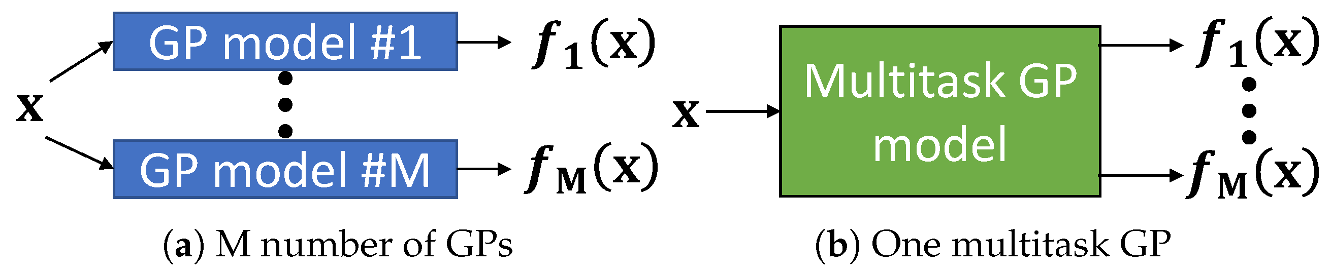
2.3. Multitask Learning

Multitask learning is a type of transfer learning in which multiple related functions (called tasks) defined over the same input variables (called domains) are simultaneously learned from the data with the objective of increasing the predictive performance of the tasks [38]. It is assumed that the feature space and the probability distribution of the domain is the same for all the task but the task itself are different. If x represents the input variable (domain), multitask learning learns multiple functions (tasks), say, f 1 ( x ) , , f M ( x ) , jointly, i.e., model p ( f 1 ( x ) , , f M ( x ) x ) , rather than learning them individually, independent of each other, i.e., model p ( f 1 ( x ) x ) , , p ( f M ( x ) x ) . This is illustrated in Figure 1.
It is easy to incorporate multitask learning into the standard GP formulation. Let X 1 , y 1 , X 2 , y 2 , …, X M , y M be the input and the output of M related tasks, such that X 1 = x 1 , 1 , , x N 1 , 1 T , X 2 = x 1 , 2 , , x N 2 , 2 T ,…, X M = x 1 , M , , x N M , M T and y 1 = y 1 , 1 , , y N 1 , 1 T , y 2 = y 1 , 2 , , y N 2 , 2 T , …, y M = y 1 , M , , y N M , M T . Here, for task 1, x 1 , 1 , , x N 1 , 1 are the N 1 vectors representing input samples and y 1 , 1 , , y N 1 , 1 are the corresponding scalar output values. Similar is the case for task 2 to M . In general, for a task t , the rows of X t ( x 1 , t , , x N t , t ) are vectors representing input samples, the elements of y t ( y 1 , t , , y N t , t ) are the corresponding scalar output values, and there are N t samples in X t and y t .
Then, if we are to collect the inputs and outputs of all of the tasks, such that X a l l = x 1 , 1 , , x N 1 , 1 , x 1 , 2 , , x N 2 , 2 , , x 1 , M , , x N M , M T and y a l l = y 1 , 1 , , y N 1 , 1 , y 1 , 2 , , y N 2 , 2 , , y 1 , M , , y N M , M T , then we could use standard GP formulation to learn a joint function that maps X a l l to y a l l , if we are able to define covariance between elements of y a l l using corresponding inputs in X a l l .
Bonilla et al. proposed using (7) to compute covariance in multitask GP prior [39].
f l ( x i , l ) , f k ( x j , k ) = K l , k f k ( x i , l , x j , k ) ,
f l ( x i , l ) , f k ( x j , k ) is the covariance between the noise-less outputs of i-th sample of task l (i.e., f l ( x i , l ) ) and j-th sample of task k (i.e., f k ( x j , k ) ). k x , x is a covariance function. K f is a M × M task covariance matrix. The task covariance matrix has to be PSD. K l , k f is the l-th row and k-th column element of K f and scales the covariance function value between the samples belonging to l-th task and k-th task, with higher magnitude implying greater relationship between the tasks. The method by Bonilla et al. [39] treats the elements of K f as hyperparameters of the model which are optimized alongside of the hyperparameters of the covariance function and noise variances. So this method automatically learns the relationship between the tasks without any supervision. However, since K f has to be a PSD matrix, it should be constrained accordingly during optimization.
y i , 1 y i , M N f l ( x i , 1 ) f l ( x i , M ) , σ 1 2 0 0 0 0 0 0 σ M 2
The likelihood function used by this method is given in (8). y i , 1 ,… , y i , M are the noisy output values which are conditioned on the noiseless output values, f l ( x i , 1 ) , , f l ( x i , M ) . It is assumed that same noise variance is observed in all the samples belonging to a task. σ 1 2 , …, σ M 2 are noise variances in tasks 1, …, M respectively. Rakitsch et al. extended this method by assuming the noise across the task to be correlated [40]. They claim such model is better suited if there are hidden factors affecting the output variables. Their method uses same prior (i.e., (7)) but uses (9) as the likelihood function. Σ Noise is a M × M noise covariance matrix which is a PSD matrix that captures relationship between the noise variance in the tasks. The elements of Σ Noise are also hyperparameters of the model.
y i , 1 y i , M N f l ( x i , 1 ) f l ( x i , M ) , Σ Noise
The learning and inference in these models can be performed similar to that for standard GP algorithm by computing covariance between samples in y a l l using (7), and noise in the observation from (8) for the first model [39] and (9) for the second [40].
Several other types of multitask GPs have been proposed in literature. They are based on approaches such as sparse linear combination of independent single-task GPs [41], multi-kernel method [42], convolved latent processes [43], and spectral mixture kernels [44]. There are also asymmetric multitask GPs, which model several tasks together with the objective of enhancing the predictions of only a subset of the tasks by transferring information from other tasks to them [45]. Readers who are interested in learning more about advanced multitask GPs are encourage to read the article by Liu et al. [46]. It reviews and experimentally compares a variety of state-of-the-art multitask GPs.

3. Datasets

We experiment with three real hyperspectral biophysical parameter prediction datasets and one synthetic dataset.

3.1. Algae Dataset

The first dataset, which we call Algae dataset, contains 103 reflectance spectra of sediments containing algal bio-films, and the contents of the chlorophyll-a, the chlorophyll-b and the carbohydrates in μ g   cm 2 . This dataset was acquired by Murphy et al. [47] from two mudflats, each of an area about 500 m2, in Sydney, Australia. The reflectance spectra covers visible and near infrared region (350–1050 n m at 1 n m interval) and was measured by an Analytical Spectral Devices (ASD) FieldSpec Pro spectroradiometer.

3.2. NEON Dataset

The second dataset, which we call NEON dataset, contains 54 reflectance spectra of foliage and the corresponding nitrogen and carbon contents of the samples, measured in terms of percentage dry foliage weight. It was collected by The National Ecological Observatory Network (NEON) [48] as part of their 2013 field campaign at San Joaquin, Soaproot Saddle, and Teakettle in California, USA [49]. It contains visible to shortwave infrared spectra (350–2500 n m at 1 n m interval) collected by an Analytical Spectral Devices (ASD) Fieldspec-3 portable field spectrometer. We also use a hyperspectral image obtained from NEON for qualitative analysis. This test image is a subset of hyperspectral data collected by NEON Imaging Spectrometer (NIS) over San Joaquin, California. It covers an area of 250 m × 250 m and each pixel has a spectral range of 382 n m to 2511 n m and has a ground sampling distance of 1 m .

3.3. SPARC Dataset

The SPARC dataset contains 118 spectra extracted from the pixels of images captured by an airborne HyMap sensor and the corresponding ground truth measurements of leaf chlorophyll (chlorophyll) in μ g   cm 2 , leaf area index (LAI) in m2 m−2, and fractional vegetation cover (fCover) in m2 m−2. Few of the ground truth values for each biophysical parameter is missing in the dataset. Such instances were ignored during experimental evaluation. The data was collected by European Space Agency (ESA) as part of their SPARC campaign around an agricultural site in Barrax, Spain [50].

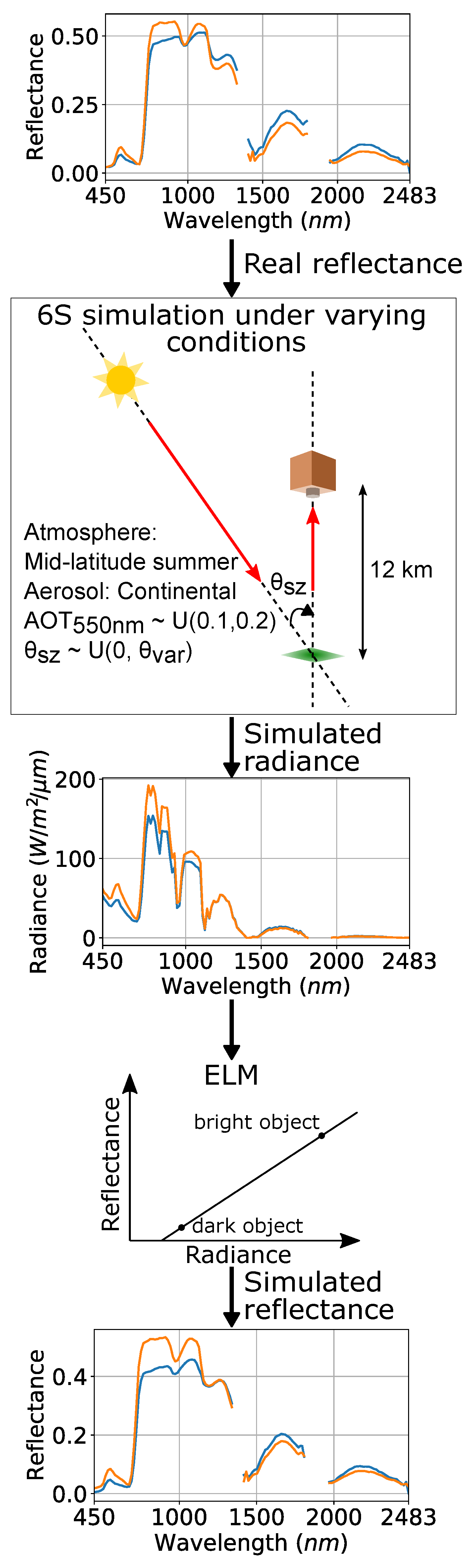
3.4. Synthetic Dataset

We propose a pipeline (shown in Figure 2) to generate synthetic datasets with varying levels of illumination variations. The goal is create datasets that can be used to compare the sensitivity of the predictive models to illumination variations. This is hard to test in real data because it will require collection of a new dataset that measures reflectance of same set of materials under varying lighting conditions whose variability can be controlled. Theoretically, reflectance should be independent of illumination variations. However, since there are no instrument to directly measure reflectance, it has to be estimated from measured radiance, sun-sensor geometry, and atmospheric conditions. This makes estimated reflectance sensitive to variation in illumination or any change in atmospheric condition [51].
The proposed simulation pipeline utilizes data from SPARC dataset, 6S atmospheric radiative transfer model [52] and empirical line method (ELM) [53]. The basic idea is to convert the reflectance spectra in SPARC dataset to a radiance observed by a hypothetical sensor defined in a 6S simulation and convert the radiance back to reflectance using ELM. We randomly vary the atmospheric parameters in the 6S simulation for each sample in SPARC dataset to introduce illumination variations in the dataset. The ELM is calibrated only once and used to retrieve reflectance for radiances simulated for different atmospheric conditions. If we allow the parameters to vary a lot, we get a dataset with artifacts of huge illumination variation and if we allow the parameters to vary by only a small amount, we have a dataset with artifacts of small illumination variations. In real-world, similar situation could arrive when reference spectra to calibrate atmospheric compensation algorithm is collected only once in the beginning of data collection and all the data collected over a long period is converted to reflectance under that calibration. In fact, such artifacts always appear when a more complex model (real atmosphere in real-world and 6S in our pipeline) is inverted by a simpler model (RTM code/ELM in real-world and ELM in our pipeline), since all the variabilities of the complex model is not captured by the simpler model. The details of the synthetic data generation process is given below.
Most of the parameters of the 6S simulation are fixed. We set the altitude to be 12 k m , atmosphere to be mid-latitude summer, aerosol profile to be Continental and the sensor to be nadir viewing. Only two parameters (AOT550 n m and solar zenith) are varied. AOT550 n m is assigned a value uniformly sampled at random from the range 0.1 to 0.2. This parameter induces noise in the radiance. The zenith angle ( θ s z ) is sampled uniformly at random from the range 0 to θ v a r . The parameter θ v a r controls the amount of spectral variability. With higher value meaning higher variability. It is held constant for one pass through the dataset. The ELM is calibrated only once for each run through the entire dataset using all zero and all one reflectance. We generate 9 separate datasets, with increasing spectral variabilities due to illumination changes, by setting θ v a r from 10° to 90° at 10° increments and running the simulation through every sample in the SPARC dataset.

4. Experimental Results

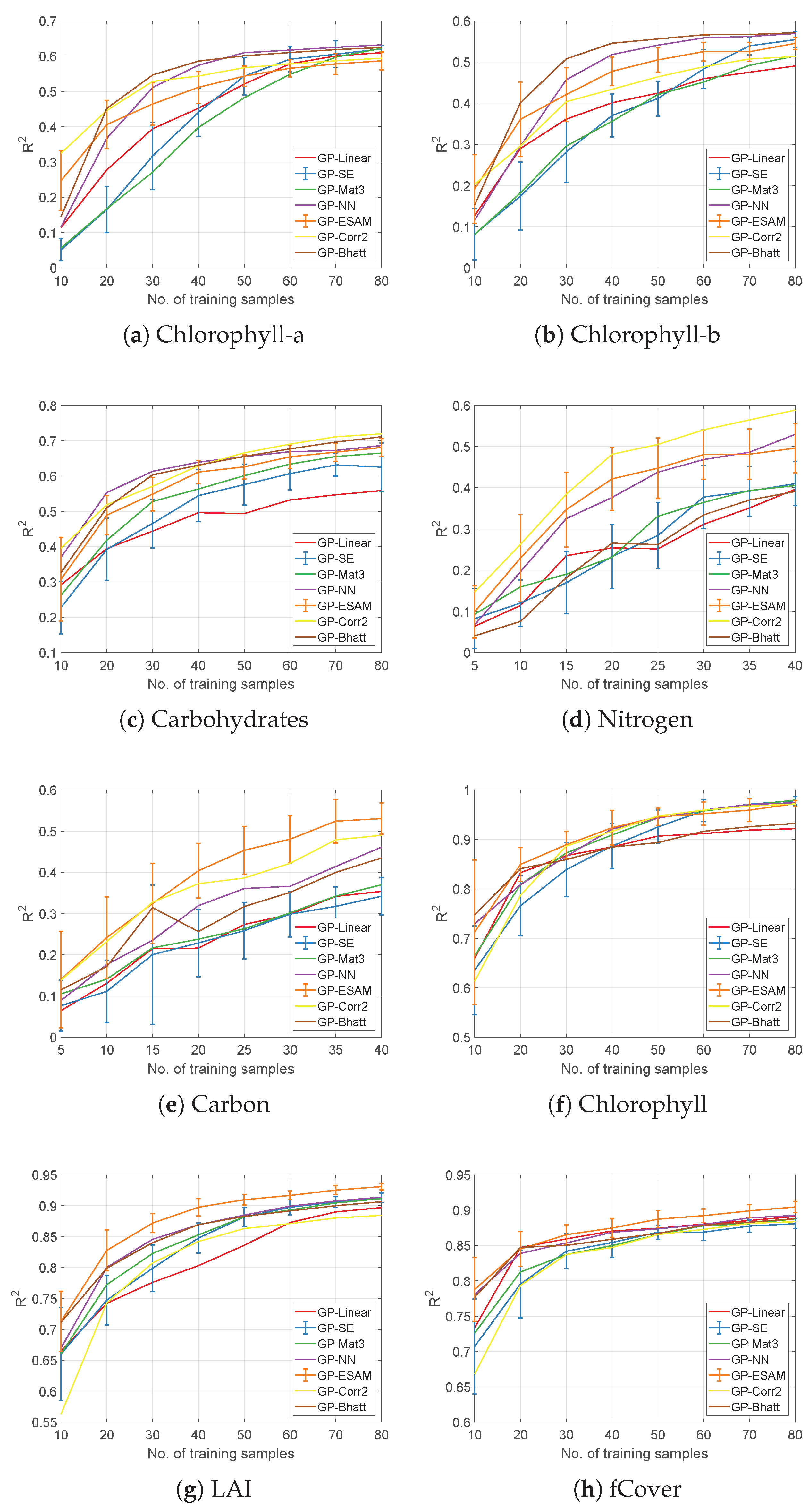
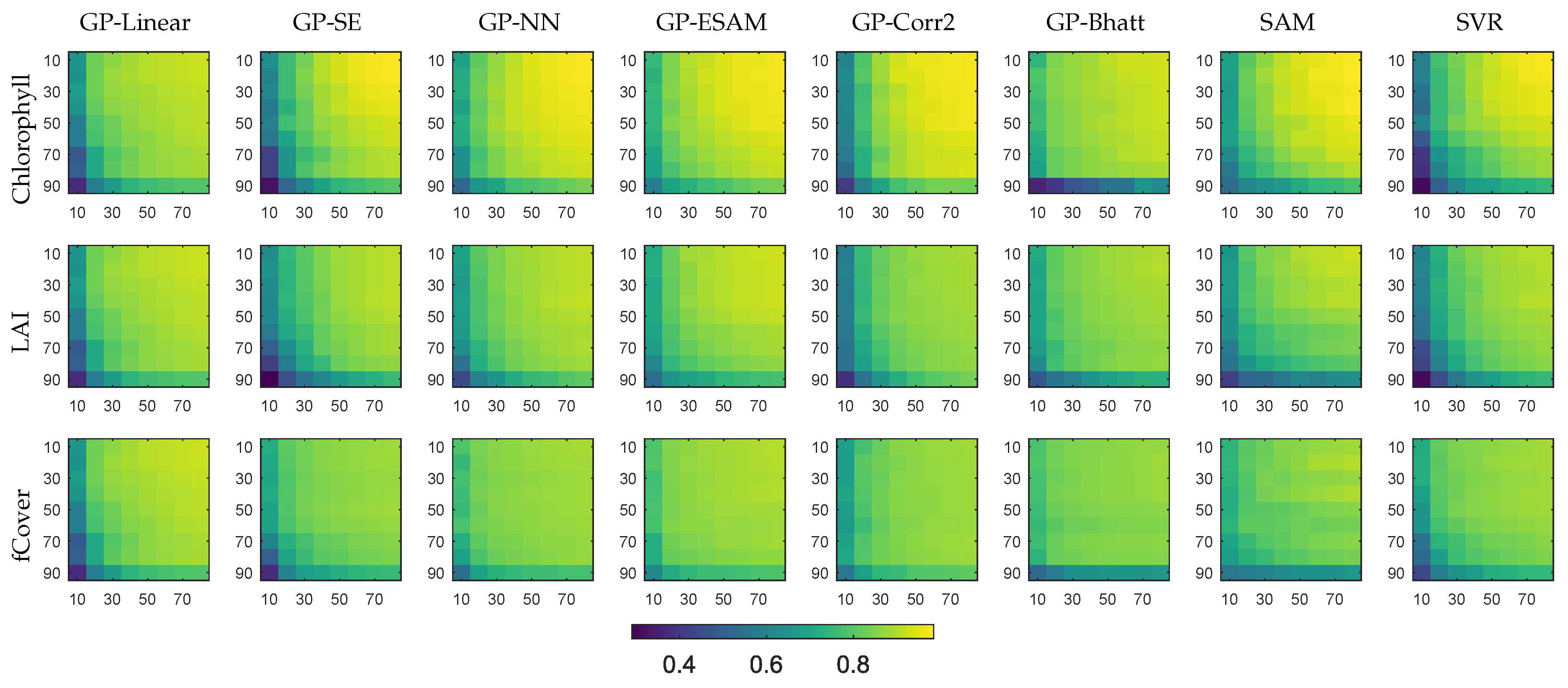
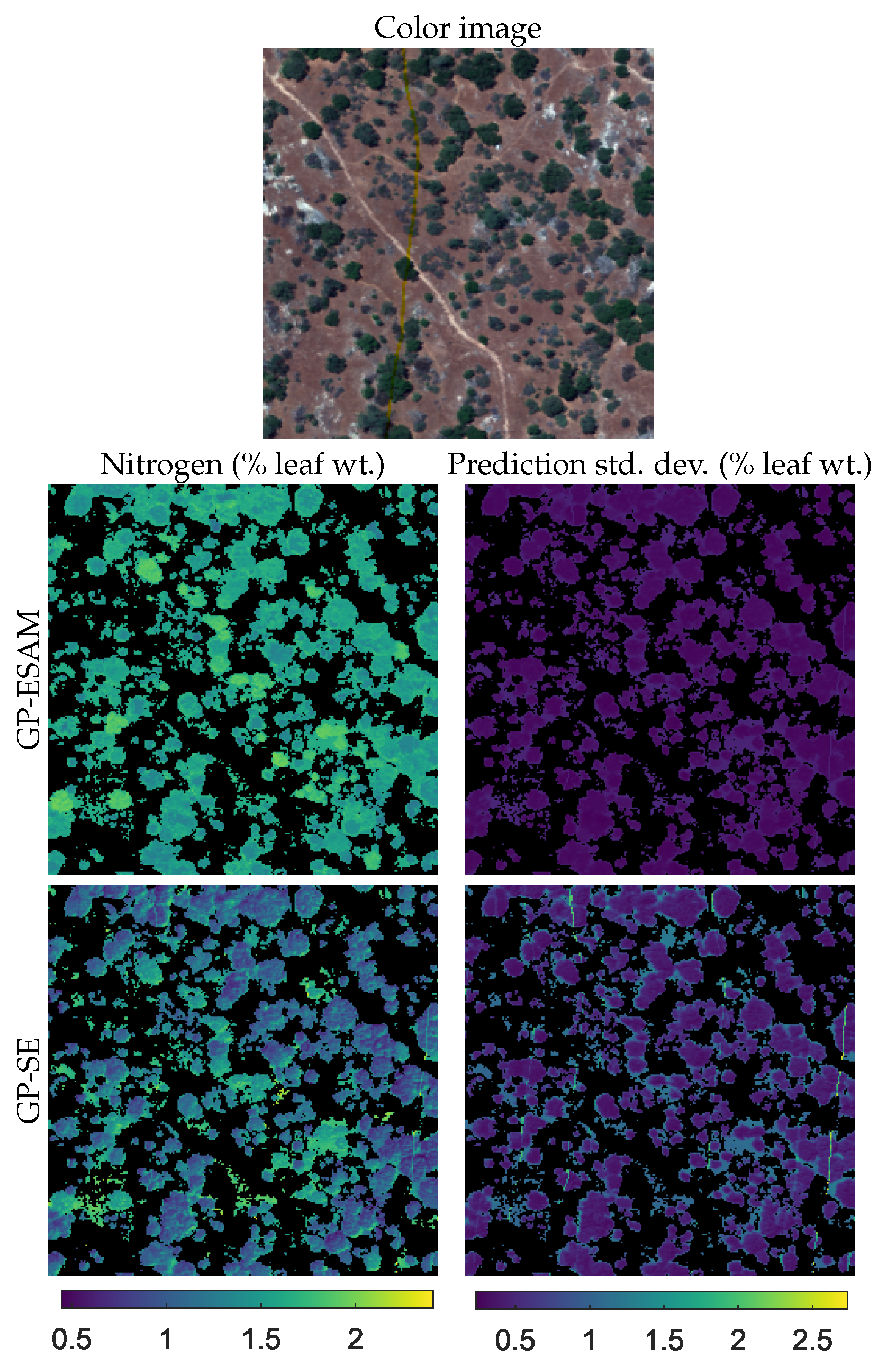
4.1. Evaluation of Covariance Functions

In this subsection, we evaluate the predictive performance of different covariance functions. The first experiment compares the predictive performance of all discussed covariance function on entirety of all three real datasets. In the second experiment, we measure the effects of training set size on the performance of the methods using the real datasets. The third experiment measures the sensitivity of predictive performances of different methods to training set size and illumination variability using the synthetic dataset. All of the results in this subsection were computed by repeating 10-fold cross-validation 30 times and reporting the mean and the standard deviation of the performance metrics over those 30 repeats. The metrics reported are the coefficient of determination ( R 2 ) and the root mean squared error (RMSE) between the prediction and the ground truth. In all of the experiments in this paper, we have not used automatic relevance determination (ARD) in covariance functions, even though previous studies [7,8] have found them useful. This is because when training on very small datasets the number of new hyperparameters introduced by ARD for spectral data usually far exceeds the dataset size. The hyperparameters of the GPs were optimized by minimizing the negative log-likelihood function using quasi-Newton method. To prevent local minima, multiple optimization trials with random initial guesses, sampled from 10 5 , 10 5 , were performed.
Table 3 and Table 4 compare the predictive performance of different methods on the real datasets. The covariance functions compared are the squared exponential (SE), the exponential (Exp), the Matern 3/2 (Mat3), the Matern 5/2 (Mat5), the linear (Linear), the polynomial of order 2 (Poly2), the polynomial of order 3 (Poly3), the neural network, the exponential spectral angle mapper (ESAM), the observation angle dependent (OAD), the correlation (Corr1), the exponential correlation (Corr2), the spectral information divergence (SID), the Bhattacharya (Bhatt), and the chi-squared (Chi2) functions. As baselines methods, we have included partial least squared (PLS), random forest (RF), spectral angle mapper (SAM), support vector regression (SVR), and kernel ridge regression (KRR). The hyperparameters of the random forest (the number of trees) and partial least squares were (the number of components) were tuned using cross-validation of the training data. For support vector regression and kernel ridge regression, we utilized the simpleR toolbox [54] implementations with squared exponential kernels, which have been used by previous studies for vegetation parameter estimation [55,56]. We also compare the results with state-of-the-art approaches for vegetation parameter prediction, i.e., VHGPR [16], GP-BAT [57], PLS-GPR [58], and WGP [59]. VHGPR was implemented using the simpleR toolbox [54]; GP-BAT and WGP were implemented using GPML toolbox [60]; and PLS-GPR was implemented using the simpleR [54] and the simFeat [61] toolboxes. The best performing method and any method which was not statistically different from the best method (two sample t-test, α = 0.01 ) have been highlighted in the table.
Comparison between spectral and other covariance function: The results show that spectral covariance functions performed the best. The non-stationary covariance functions in general outperformed the stationary covariance functions (including the squared exponential function which was used by most of the previous studies). This is due to the fact that the Euclidean distance between the spectra is not good metric for similarity for spectral data. Our results prove that when applying Gaussian processes for vegetation parameter estimation, rather than just utilizing the default squared exponential covariance function as done by previous studies, it would be wise to use model selection techniques, such as cross validation, to choose the best non-stationary covariance function.
Comparison with baselines: GP based methods performed superior to the baselines, except for Chlorophyll prediction in SPARC dataset, for which surprisingly SAM performed the best. The comparison of GP based methods with SAM for SPARC dataset’s Chlorophyll prediction will be examined again in the third experiment.
Comparison with the state-of-the-art: When comparing with the state-of-the-art approaches, GP with spectral covariance functions mostly performed better than VHGPR and WGP, which are methods that utilize squared exponential covariance function with more advanced likelihood functions. Additionally, the proposed methods outperformed band selection (GP-BAT) and dimensionality reduction (PLS-GPR) based methods. In addition to the state-of-the-art methods listed in the table, we also experimented with a recent deep learning based biophysical/biochemical parameter prediction network, called DeepSpectra [21]. The exact network architecture experimented was the one used to predict corn protein in the DeepSpectra paper. In our experiments, we found that the validation loss did not converge, even when the training loss converged, for NEON dataset (the smallest dataset), and for Chlorophyll-a and Chlorophyll-b in Algae dataset. For rest of the parameters, the model produced poor results. The R 2 of prediction for Carbohydrate in Algae dataset was 0.6459 ± 0.0392 and the R 2 of prediction for Chlorophyll, LAI, and fCover in SPARC dataset were 0.9114 ± 0.0179, 0.8848 ± 0.0149, and 0.8783 ± 0.0170, respectively. This clearly indicates that that DeepSpectra model was over-fitting on our datasets. We tried increasing the regularization by increasing the weight decay value, increasing the dropout rate and decreasing the number of hidden units, but no performance increase was observed. We hypothesize that the difficulty in training is due to the fact that the training set size of our dataset is smaller and our datasets are much noisier than the ones used in the DeepSpectra paper. Better results could be obtained by further tuning the hyperparameters of the network and making changes to network architecture, but that is beyond the scope of our study. This shows another benefit of GPs that they have fewer number of hyperparameters, which can be automatically learned by minimizing log-likelihood function using an optimizer.
In the next experiment, we test how the performance of the models vary with training set size. The results are shown in Figure 3. Since, both R 2 and R M S E performance metrics showed congruent results in the first experiment, only R 2 metric is reported in the remainder of the paper. The performance curves were obtained by using a modified form of repeated 10 fold cross-validation. In each iteration of the cross-validation, the models were trained on only a random subset of the samples in the training fold. The size of the subset was set to the training set size for which performance is desired to be measured. By varying the size of the subset, the performance as function of training set size was obtained. This process guarantees that the size of the test set is same, even though the size of the training set is varying, so that the results obtained from models trained on training sets of different sizes can be compared. In this experiment, we did not exhaustively cover all of the covariance functions, but only chose a representative set. Only standard deviations of the squared exponential covariance function and the exponential spectral angle mapper are shown for comparison.
The plots again show that the non-stationary functions are better. In general, we find that the gap in performance between stationary covariance functions and non-stationary covariance functions is larger when the training set size is small. This gap slowly narrows as the number of training examples is increased. This shows that non-stationary covariance functions (spectral functions in particular) are more preferable for biophysical prediction when the ground truth is limited. From the plots, we can extrapolate that if we have large quantity of ground truth, there would not be difference in performance between stationary and non-stationary covariance functions. This observation is in agreement with the theory of Bayesian methods that states that as the amount of data available grows to be sufficiently large, the effects of prior tend toward becoming irrelevant, provided the prior does not make strong incorrect assumptions about the data [62]. It should be noted that the phenomenon of narrowing of the performance gap as training set size is increased is not seen in biophysical parameters from NEON dataset. This could be happening because of the fact that, among the three datasets, this is the smallest one and with even the full dataset used for training, the training set is not adequate to properly model the relationship. This claim is supported by the fact that in other datasets the performance tend to taper off and the standard deviation of performance rapidly diminishes as the number of sample used tends to be as large as the entire dataset, but this is not observed for biophysical parameters from the NEON dataset.
Figure 4 shows the results of the third experiment that utilizes the synthetic dataset to show the effects of illumination variations and size of training set. The mean R 2 metric over 30 repeats of 10-fold cross validation is shown in the figure. We have used 9 synthetic datasets obtained by setting θ v a r values from 0° to 90°. Each of those used the same procedure as the last experiment to obtained performance under varying training set size. The results indicate that non-stationary covariance functions (in particular spectral covariance functions) perform better not only under limited ground truth but also when illumination variation is high in the training set. One surprising result obtained in Table 3 and Table 4 was that SAM performed better than Gaussian process based method when predicting chlorophyll in SPARC dataset. Figure 4 proves that when the training set is limited or illumination variation is high the non-stationary covariance functions outshine the SAM. This is because SAM, which is basically a nearest neighbor method with cosine similarity as distance metric, needs large set of training data to work properly as it makes hard decision to assign the test sample to the closest training set sample. If the gap between the training set is large, the error is high for SAM but GP can learn a smooth function between the gap to reduce the prediction error.
In Figure 5, we qualitatively compare leaf nitrogen maps produced using GP-SE and GP-ESAM models trained on the NEON dataset. The test image was acquired by NEON imaging spectrometer (NIS) over an area in San Joaquin, California. Since, the NEON dataset contains leaf spectra, we use 4SAIL canopy model [63] to generate synthetic canopy spectra from NEON dataset for training. Two hundred and fifty training samples were generated by randomly selecting samples from the NEON dataset and passing it through the 4SAIL model. The parameters of 4SAIL model was set as follows. The solar zenith, the solar azimuth and the range of values for the viewing zenith and the viewing azimuth from which they were randomly sampled from were obtained from the meta-information in the test image file. Other parameters were uniformly sampled at random from a range–leaf area index: 0.1 to 4.0, average leaf angle: 10° to 80°, hot spot parameter: 0.01 to 1.0, and soil brightness factor: 0.1 to 1.0. The reflectance and the transmittance of the leaf required by 4SAIL were estimated using the method in [64] using the leaf reflectance against a white background and the same against a black background, present in the NEON dataset. We resample the bands of training samples to match with the imaging spectrometers bands and remove the water bands. Non-vegetation pixels in the images have been blacked out. We see that the maps produced by the two methods are different. Unfortunately, there are no ground truth measurements corresponding to the pixels of the image to quantitatively compare the performance of the methods.

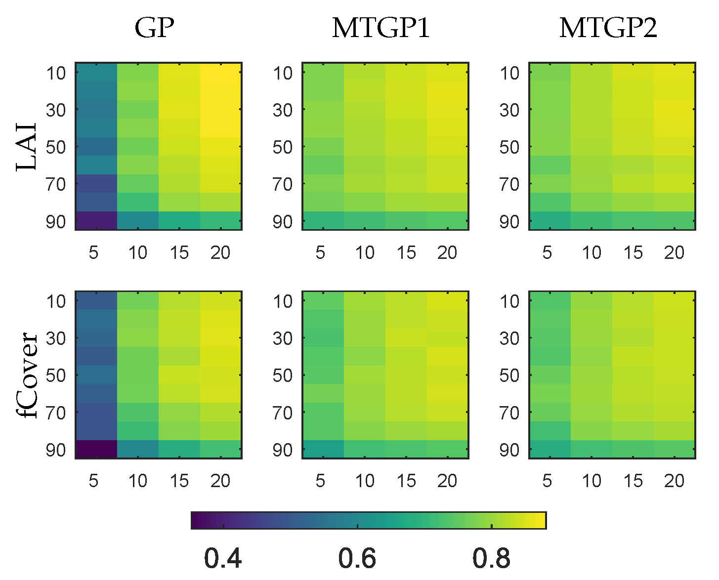
4.2. Evaluation of Multitask Gaussian Processes

In this section, we experiment on the real datasets and the synthetic dataset to show the benefits of multitask learning. We experiment with two vegetation parameters from each dataset at a time. The vegetation parameter of interest is called the primary vegetation parameter and the other is called secondary vegetation parameter. We assume that we have limited ground truth for the primary vegetation parameter but have larger quantity of ground truth for the secondary vegetation parameter. We follow the same evaluation methodology as in the previous experiments to obtain performance as a function of primary vegetation parameter’s training set size. The only difference is that in each cross-validation iteration within 30 random trials only the ground truth of the primary vegetation parameter is subsetted from the training fold while all of the training fold ground truth of the secondary vegetation parameter is kept. So each model is trained on spectra in the training fold which have secondary vegetation parameter ground truth for all of its samples but have primary biophysical parameter ground truth for only a subset. The models are tested on separate set on spectra in the testing fold. For Algae and SPARC datasets, which have 3 vegetation parameters, we evaluate every combination of pair of parameters.
In the remainder of this paper, the multitask model [39] proposed by Bonilla et al. is referred as MTGP1 and the multitask model [40] by Rakitsch et al. is referred as MTGP2. Gaussian processes modeling only one task is referred as single-task GP or GP. To uniformly compare the multitask models, we set the covariance function to ESAM throughout the experiments. To make sure that K f , and also Σ M × M for MTGP2, are PSD, they are parameterized as i = 1 r a i a i T + c 2 I M × M , where a i i are M dimensional vectors, c is a scalar, r is an integer whose value can range from 1 to M . This approximation generally produces a PSD matrix because the diagonal of the approximation generally have higher magnitude than the rest of the elements [40]. a i ’s and c are learned from the data with other hyperparameters. The value of r controls the rank and the number of hyperparameters associated with K f and Σ M × M . During training, we learn M separate models by one-by-one setting the value of r to values in the range 1 to M and tuning the hyperparameters of the model using the same procedure as the one used for GPs in previous experiments. Out of the M models, the one which exhibits the lowest negative log-likelihood value is picked as the final model.
Table 5 and Table 6 compare single-task GP and multitask GP. Table 5 shows the combinations of vegetation parameters which benefited from multitask learning and Table 6 shows the combinations that did not. The results for each vegetation parameter was obtained by considering it as the primary vegetation parameter and the other vegetation parameter as the secondary. For Algae dataset, multitask learning of chlorophyll-a and chlorophyll-b was beneficial but learning either of them with carbohydrate was not. This could be because chlorophyll-a and chlorophyll-b are more similar because both of them are pigments. The joint modeling of leaf nitrogen and leaf carbon was seen to be beneficial in NEON dataset. For SPARC dataset, multitask learning of leaf area index and fractional vegetation cover performed better but either did not benefit from joint modeling with leaf chlorophyll content. This is expected because leaf area index and fractional vegetation cover are known to be related [65] but there is no direct relationship of either with the leaf chlorophyll contents. For the positive results, the gain in performance is the largest when the training set size of the primary biophysical parameter is lowest, and steady grows as it is increased. When the primary vegetation parameter’s training set size is adequately large, we see that there is no gain from using multitask GP. The best performing model and any model which was not statistically different from the best model (two sample t-test, α = 0.01 ) have been highlighted in the table. Since experiments with pairs of vegetation parameters in Algae and SPARC dataset did not show that all three vegetation parameters in the dataset are related, we did not experiment with modeling three vegetation parameters jointly with multitask learning. However, the same approach can be used to learn more than two vegetation parameters together.
Now, we investigate whether multitask learning can be used to improve the prediction of model when the illumination variation in the training dataset is high. For this, we again utilize the synthetic dataset. As in previous experiments, Figure 6 shows the variation of R 2 metric as function of training set size and illumination variation for single-task and multitask GPs. We observe that multitask GP outperforms single-task GP, when either training set size is small and/or illumination variations is high.

5. Conclusions

The performance of the vegetation parameter prediction models is generally limited by the size of the training set. This paper applied two Gaussian processes based techniques for retrieval of vegetation parameters from hyperspectral imagery when the training set is small and evaluated those approaches on real and synthetic data. First, we showed that compared to the popularly used squared exponential covariance function, non-stationary covariance functions, in particular spectral covariance functions, can provide better prediction, especially when the training set is small or has high spectral variability. Spectral covariance functions are those which are based on well-established spectral comparison metrics, such as spectral angle and spectral correlation. Spectral covariance functions performed better because they provide better prior for Gaussian process regression as spectral metrics are better for comparing similarity between the spectra than Euclidean distance on which many commonly used covariance functions are based. Since spectral metrics are less affected by spectral variations due to factors, such as changes in illumination, the Gaussian process models that used spectral covariance functions also showed better resilience to spectral variability.
The second idea presented is joint modeling of multiple related vegetation parameters by a multitask Gaussian process. In the experiments, we proved that prediction of a vegetation parameter whose training set is small or has large spectral variations can be improved by jointly learning their model with prediction models for related vegetation parameters. This approach showed best result when the ground truth for related vegetation parameter was much larger than ground truth of the vegetation parameter of interest. This approach can handle joint modeling of several vegetation parameters, but our experimental evaluation was limited to modeling only two vegetation parameters because only two parameters showed relationship in all of the datasets. Modeling of more than two parameters jointly needs to be investigated in future studies. As the number of vegetation parameters is increased so does the training set size of the multitask GP, therefore scalable models, such as sparse Gaussian processes [66,67,68], could be used for efficient learning and inference when modeling several vegetation parameters. We would also like to compare the performance of the two multitask Gaussian processes used in our experiments to other state-of-the-art multitask Gaussian processes for the task of predicting vegetation parameters. We are especially interested to investigate whether asymmetric multitask models [45], which prioritize better modeling of variables of interest, are better than symmetric multitask models like the ones used in our experiments, which give equal priority to all modeled variables. Similarly, it would be interesting to combine the proposed methods with previously existing approaches for handling scarce training set, i.e., active learning scheme and fusion with radiative transfer models, to possibly further improve the prediction accuracy.

Author Contributions

U.B.G. wrote the manuscript. U.B.G., S.T.M., and E.S. conceptualized and contributed to the algorithmic methods.

Funding

This research was partially supported by the Department of Defense and an Amazon AWS in Education Machine Learning Grant.

Acknowledgments

The authors would like to thank Richard J. Murphy for providing the Algae dataset, Jan van Aardt for providing the NEON dataset, and Jochem Verrelst for providing the processed SPARC dataset.

Conflicts of Interest

The authors declare no conflict of interest.

References

  1. Verrelst, J.; Malenovskỳ, Z.; Van der Tol, C.; Camps-Valls, G.; Gastellu-Etchegorry, J.P.; Lewis, P.; North, P.; Moreno, J. Quantifying Vegetation Biophysical Variables from Imaging Spectroscopy Data: A Review on Retrieval Methods. Surv. Geophys. 2019, 40, 589–629. [Google Scholar] [CrossRef]
  2. Eismann, M.T. Hyperspectral Remote Sensing; SPIE Press: Bellingham, WA, USA, 2012. [Google Scholar]
  3. Ramoelo, A.; Skidmore, A.; Cho, M.; Mathieu, R.; Heitkönig, I.; Dudeni-Tlhone, N.; Schlerf, M.; Prins, H. Non-linear partial least square regression increases the estimation accuracy of grass nitrogen and phosphorus using in situ hyperspectral and environmental data. ISPRS J. Photogramm. Remote Sens. 2013, 82, 27–40. [Google Scholar] [CrossRef]
  4. Darvishzadeh, R.; Skidmore, A.; Schlerf, M.; Atzberger, C.; Corsi, F.; Cho, M. LAI and chlorophyll estimation for a heterogeneous grassland using hyperspectral measurements. ISPRS J. Photogramm. Remote Sens. 2008, 63, 409–426. [Google Scholar] [CrossRef]
  5. Verrelst, J.; Muñoz-Marí, J.; Alonso, L.; Delegido, J.; Rivera, J.P.; Camps-Valls, G.; Moreno, J. Machine learning regression algorithms for biophysical parameter retrieval: Opportunities for Sentinel-2 and -3. Remote Sens. Environ. 2012, 118, 127–139. [Google Scholar] [CrossRef]
  6. Camps-Valls, G.; Muñoz-Marí, J.; Gómez-Chova, L.; Richter, K.; Calpe-Maravilla, J. Biophysical parameter estimation with a semisupervised support vector machine. IEEE Geosci. Remote Sens. Lett. 2009, 6, 248–252. [Google Scholar] [CrossRef]
  7. Verrelst, J.; Alonso, L.; Caicedo, J.P.R.; Moreno, J.; Camps-Valls, G. Gaussian process retrieval of chlorophyll content from imaging spectroscopy data. IEEE J. Sel. Top. Appl. Earth Obs. Remote Sens. 2013, 6, 867–874. [Google Scholar] [CrossRef]
  8. Verrelst, J.; Alonso, L.; Camps-Valls, G.; Delegido, J.; Moreno, J. Retrieval of Vegetation Biophysical Parameters Using Gaussian Process Techniques. IEEE Trans. Geosci. Remote Sens. 2012, 50, 1832–1843. [Google Scholar] [CrossRef]
  9. Pasolli, E.; Melgani, F.; Alajlan, N.; Bazi, Y. Active learning methods for biophysical parameter estimation. IEEE Trans. Geosci. Remote Sens. 2012, 50, 4071–4084. [Google Scholar] [CrossRef]
  10. Bannari, A.; Morin, D.; Bonn, F.; Huete, A. A review of vegetation indices. Remote Sens. Rev. 1995, 13, 95–120. [Google Scholar] [CrossRef]
  11. Pasqualotto, N.; Delegido, J.; Van Wittenberghe, S.; Verrelst, J.; Rivera, J.P.; Moreno, J. Retrieval of canopy water content of different crop types with two new hyperspectral indices: Water Absorption Area Index and Depth Water Index. Int. J. Appl. Earth Obs. Geoinf. 2018, 67, 69–78. [Google Scholar] [CrossRef]
  12. Jacquemoud, S.; Verhoef, W.; Baret, F.; Bacour, C.; Zarco-Tejada, P.J.; Asner, G.P.; François, C.; Ustin, S.L. PROSPECT+ SAIL models: A review of use for vegetation characterization. Remote Sens. Environ. 2009, 113, S56–S66. [Google Scholar] [CrossRef]
  13. Gewali, U.B.; Monteiro, S.T.; Saber, E. Machine learning based hyperspectral image analysis: A survey. arXiv 2018, arXiv:1802.08701. [Google Scholar]
  14. Camps-Valls, G.; Verrelst, J.; Muñoz-Marí, J.; Laparra, V.; Mateo-Jimenez, F.; Gomez-Dans, J. A Survey on Gaussian Processes for Earth-Observation Data Analysis: A Comprehensive Investigation. IEEE Geosci. Remote Sens. Mag. 2016, 4, 58–78. [Google Scholar] [CrossRef] [Green Version]
  15. Pasolli, L.; Melgani, F.; Blanzieri, E. Gaussian process regression for estimating chlorophyll concentration in subsurface waters from remote sensing data. IEEE Geosci. Remote Sens. Lett. 2010, 7, 464–468. [Google Scholar] [CrossRef]
  16. Lázaro-Gredilla, M.; Titsias, M.K.; Verrelst, J.; Camps-Valls, G. Retrieval of biophysical parameters with heteroscedastic Gaussian processes. IEEE Geosci. Remote Sens. Lett. 2014, 11, 838–842. [Google Scholar] [CrossRef]
  17. Bazi, Y.; Melgani, F. Semisupervised Gaussian process regression for biophysical parameter estimation. In Proceedings of the IEEE International Geoscience and Remote Sensing Symposium (IGARSS), Honolulu, HI, USA, 25–30 July 2010; pp. 4248–4251. [Google Scholar] [CrossRef]
  18. Muñoz-Marí, J.; Verrelst, J.; Lázaro-Gredilla, M.; Camps-Vails, G. Biophysical parameter retrieval with warped Gaussian processes. In Proceedings of the International Geoscience and Remote Sensing Symposium (IGARSS), Milan, Italy, 26–31 July 2015; pp. 13–16. [Google Scholar]
  19. Svendsen, D.H.; Martino, L.; Campos-Taberner, M.; García-Haro, F.J.; Camps-Valls, G. Joint Gaussian processes for biophysical parameter retrieval. IEEE Trans. Geosci. Remote Sens. 2018, 56, 1718–1727. [Google Scholar] [CrossRef]
  20. Ni, C.; Wang, D.; Tao, Y. Variable weighted convolutional neural network for the nitrogen content quantization of Masson pine seedling leaves with near-infrared spectroscopy. Spectrochim. Acta Part A Mol. Biomol. Spectrosc. 2019, 209, 32–39. [Google Scholar] [CrossRef]
  21. Zhang, X.; Lin, T.; Xu, J.; Luo, X.; Ying, Y. DeepSpectra: An end-to-end deep learning approach for quantitative spectral analysis. Anal. Chim. Acta 2019, 1058, 48–57. [Google Scholar] [CrossRef] [PubMed]
  22. Rasmussen, C.E.; Williams, C. Gaussian Processes for Machine Learning; The MIT Press: Cambridge, MA, USA, 2005. [Google Scholar]
  23. Cho, Y.; Saul, L.K. Kernel methods for deep learning. In Advances in Neural Information Processing Systems; The MIT Press: Cambridge, MA, USA, 2009; pp. 342–350. Available online: https://papers.nips.cc/paper/3628-kernel-methods-for-deep-learning (accessed on 8 May 2019).
  24. Paciorek, C.J.; Schervish, M.J. Nonstationary covariance functions for Gaussian process regression. In Advances in Neural Information Processing Systems; The MIT Press: Cambridge, MA, USA, 2004; pp. 273–280. Available online: https://papers.nips.cc/paper/2350-nonstationary-covariance-functions-for-gaussian-process-regression (accessed on 8 May 2019).
  25. Remes, S.; Heinonen, M.; Kaski, S. Non-stationary spectral kernels. In Advances in Neural Information Processing Systems; The MIT Press: Cambridge, MA, USA, 2017; pp. 4642–4651. Available online: https://papers.nips.cc/paper/7050-non-stationary-spectral-kernels (accessed on 8 May 2019).
  26. Zorzi, M.; Chiuso, A. The harmonic analysis of kernel functions. Automatica 2018, 94, 125–137. [Google Scholar] [CrossRef] [Green Version]
  27. Paciorek, C.J.; Schervish, M.J. Spatial modelling using a new class of nonstationary covariance functions. Environmetrics 2006, 17, 483–506. [Google Scholar] [CrossRef]
  28. Lang, T.; Plagemann, C.; Burgard, W. Adaptive Non-Stationary Kernel Regression for Terrain Modeling. In Robotics: Science and Systems; MIT Press: Cambridge, MA, USA, 2007; Volume 6. [Google Scholar]
  29. Zorzi, M.; Chiuso, A. Sparse plus low rank network identification: A nonparametric approach. Automatica 2017, 76, 355–366. [Google Scholar] [CrossRef] [Green Version]
  30. Van der Meer, F. The effectiveness of spectral similarity measures for the analysis of hyperspectral imagery. Int. J. Appl. Earth Obs. Geoinf. 2006, 8, 3–17. [Google Scholar] [CrossRef]
  31. Melkumyan, A.; Nettleton, E. An Observation Angle Dependent Nonstationary Covariance Function for Gaussian Process Regression. In Neural Information Processing; Lecture Notes in Computer Science; Springer: Berlin, Germany, 2009; pp. 331–339. [Google Scholar]
  32. Schneider, S.; Murphy, R.J.; Melkumyan, A. Evaluating the performance of a new classifier–the GP-OAD: A comparison with existing methods for classifying rock type and mineralogy from hyperspectral imagery. ISPRS J. Photogramm. Remote Sens. 2014, 98, 145–156. [Google Scholar] [CrossRef]
  33. Gewali, U.B.; Monteiro, S.T. A novel covariance function for predicting vegetation biochemistry from hyperspectral imagery with Gaussian processes. In Proceedings of the International Conference on Image Processing (ICIP), Phoenix, AZ, USA, 25–28 September 2016; pp. 2216–2220. [Google Scholar] [CrossRef]
  34. Jiang, H.; Ching, W.K. Correlation kernels for support vector machines classification with applications in cancer data. Comput. Math. Methods Med. 2012, 2012, 205025. [Google Scholar] [CrossRef] [PubMed]
  35. Moreno, P.J.; Ho, P.P.; Vasconcelos, N. A Kullback-Leibler divergence based kernel for SVM classification in multimedia applications. In Proceedings of the Advances in Neural Information Processing Systems (NIPS), Vancouver, BC, Canada, 13–18 December 2004; pp. 1385–1392. [Google Scholar]
  36. Chan, A.B.; Vasconcelos, N.; Moreno, P.J. A Family of Probabilistic Kernels Based on Information Divergence; Technical Report SVCL-TR-2004-1; University of California: San Diego, CA, USA, 2004. [Google Scholar]
  37. Maji, S.; Berg, A.C.; Malik, J. Efficient classification for additive kernel SVMs. IEEE Trans. Pattern Anal. Mach. Intell. 2013, 35, 66–77. [Google Scholar] [CrossRef] [PubMed]
  38. Pan, S.J.; Yang, Q. A survey on transfer learning. IEEE Trans. Knowl. Data Eng. 2010, 22, 1345–1359. [Google Scholar] [CrossRef]
  39. Bonilla, E.V.; Chai, K.M.; Williams, C. Multi-task Gaussian process prediction. In Advances in Neural Information Processing Systems; The MIT Press: Cambridge, MA, USA, 2008; pp. 153–160. Available online: https://papers.nips.cc/paper/3189-multi-task-gaussian-process-prediction (accessed on 8 May 2019).
  40. Rakitsch, B.; Lippert, C.; Borgwardt, K.; Stegle, O. It is all in the noise: Efficient multi-task Gaussian process inference with structured residuals. In Advances in Neural Information Processing Systems (NIPS); The MIT Press: Cambridge, MA, USA, 2013; pp. 1466–1474. Available online: https://papers.nips.cc/paper/5089-it-is-all-in-the-noise-efficient-multi-task-gaussian-process-inference-with-structured-residuals (accessed on 8 May 2019).
  41. Nguyen, T.V.; Bonilla, E.V. Collaborative Multi-output Gaussian Processes. In Proceedings of the Uncertainty in Artificial Intelligence (UAI), Quebec City, QC, Canada, 23–27 July 2014; pp. 643–652. [Google Scholar]
  42. Melkumyan, A.; Ramos, F. Multi-kernel Gaussian processes. In Proceedings of the International Joint Conference on Artificial Intelligence (IJCAI), Barcelona, Spain, 16–22 July 2011. [Google Scholar]
  43. Álvarez, M.A.; Lawrence, N.D. Computationally efficient convolved multiple output Gaussian processes. J. Mach. Learn. Res. 2011, 12, 1459–1500. [Google Scholar]
  44. Parra, G.; Tobar, F. Spectral mixture kernels for multi-output Gaussian processes. In Proceedings of the Advances in Neural Information Processing Systems (NIPS), Long Beach, CA, USA, 4–9 December 2017; pp. 6681–6690. [Google Scholar]
  45. Leen, G.; Peltonen, J.; Kaski, S. Focused multi-task learning in a Gaussian process framework. Mach. Learn. 2012, 89, 157–182. [Google Scholar] [CrossRef]
  46. Liu, H.; Cai, J.; Ong, Y.S. Remarks on multi-output Gaussian process regression. Knowl.-Based Syst. 2018, 144, 102–121. [Google Scholar] [CrossRef]
  47. Murphy, R.J.; Tolhurst, T.J.; Chapman, M.G.; Underwood, A.J. Estimation of surface chlorophyll-a on an emersed mudflat using field spectrometry: accuracy of ratios and derivative-based approaches. Int. J. Remote Sens. 2005, 26, 1835–1859. [Google Scholar] [CrossRef]
  48. National Ecological Observatory Network (NEON). 2013. Available online: http://data.neonscience.org (accessed on 8 August 2016).
  49. Kampe, T.; Leisso, N.; Musinsky, J.; Petroy, S.; Karpowiez, B.; Krause, K.; Crocker, R.I.; DeVoe, M.; Penniman, E.; Guadagno, T.; et al. The NEON 2013 airborne campaign at domain 17 terrestrial and aquatic sites in California. In NEON Technical Memorandum Series, TM-005; National Ecological Observatory Network (NEON): Boulder, CO, USA, 2013. [Google Scholar]
  50. Moreno, J.; Alonso, L.; Fernández, G.; Fortea, J.; Gandía, S.; Guanter, L.; García, J.; Martí, J.; Melia, J.; De Coca, F.; et al. The SPECTRA Barrax Campaign (SPARC): Overview and First Results from CHRIS Data. In Proceedings of the 2nd CHRIS/Proba Workshop, Frascati, Italy, 28–30 April 2004; Available online: http://earth.esa.int/workshops/chris_proba_04/book.pdf (accessed on 8 May 2019).
  51. Teillet, P. Image correction for radiometric effects in remote sensing. Int. J. Remote Sens. 1986, 7, 1637–1651. [Google Scholar] [CrossRef]
  52. Vermote, E.F.; Tanré, D.; Deuze, J.L.; Herman, M.; Morcette, J.J. Second simulation of the satellite signal in the solar spectrum, 6S: An overview. IEEE Trans. Geosci. Remote Sens. 1997, 35, 675–686. [Google Scholar] [CrossRef]
  53. Smith, G.M.; Milton, E.J. The use of the empirical line method to calibrate remotely sensed data to reflectance. Int. J. Remote Sens. 1999, 20, 2653–2662. [Google Scholar] [CrossRef]
  54. Camps-Valls, G.; Gómez-Chova, L.; Muñoz-Marí, J.; Lázaro-Gredilla, M.; Verrelst, J. simpleR: A Simple Educational Matlab Toolbox for Statistical Regression, V2.1. 2013. Available online: http://www.uv.es/gcamps/code/simpleR.html (accessed on 20 January 2019).
  55. Caicedo, J.P.R.; Verrelst, J.; Muñoz-Marí, J.; Moreno, J.; Camps-Valls, G. Toward a semiautomatic machine learning retrieval of biophysical parameters. IEEE J. Sel. Top. Appl. Earth Obs. Remote Sens. 2014, 7, 1249–1259. [Google Scholar] [CrossRef]
  56. Verrelst, J.; Dethier, S.; Rivera, J.P.; Muñoz-Marí, J.; Camps-Valls, G.; Moreno, J. Active learning methods for efficient hybrid biophysical variable retrieval. IEEE Geosci. Remote Sens. Lett. 2016, 13, 1012–1016. [Google Scholar] [CrossRef]
  57. Verrelst, J.; Rivera, J.P.; Gitelson, A.; Delegido, J.; Moreno, J.; Camps-Valls, G. Spectral band selection for vegetation properties retrieval using Gaussian processes regression. Int. J. Appl. Earth Obs. Geoinf. 2016, 52, 554–567. [Google Scholar] [CrossRef]
  58. Rivera-Caicedo, J.P.; Verrelst, J.; Muñoz-Marí, J.; Camps-Valls, G.; Moreno, J. Hyperspectral dimensionality reduction for biophysical variable statistical retrieval. ISPRS J. Photogramm. Remote Sens. 2017, 132, 88–101. [Google Scholar] [CrossRef]
  59. Mateo-Sanchis, A.; Muñoz-Marí, J.; Pérez-Suay, A.; Camps-Valls, G. Warped Gaussian Processes in Remote Sensing Parameter Estimation and Causal Inference. IEEE Geosci. Remote Sens. Lett. 2018, 15, 1647–1651. [Google Scholar] [CrossRef]
  60. Rasmussen, C.E.; Nickisch, H. Gaussian processes for machine learning (GPML) toolbox. J. Mach. Learn. Res. 2010, 11, 3011–3015. [Google Scholar]
  61. Izquierdo-Verdiguier, E.; Gómez-Chova, L.; Camps-Valls, G.; Muñoz-Marí, J. simFeat 2.2: MATLAB Feature Extraction Toolbox. Available online: https://github.com/IPL-UV/simFeat (accessed on 2 April 2019).
  62. Bishop, C.M. Pattern Recognition and Machine Learning (Information Science and Statistics); Springer: Berlin/Heidelberg, Germany, 2006. [Google Scholar]
  63. Verhoef, W.; Jia, L.; Xiao, Q.; Su, Z. Unified optical-thermal four-stream radiative transfer theory for homogeneous vegetation canopies. IEEE Trans. Geosci. Remote Sens. 2007, 45, 1808–1822. [Google Scholar] [CrossRef]
  64. Major, D.J.; McGinn, S.M.; Gillespie, T.J.; Baret, F. A technique for determination of single leaf reflectance and transmittance in field studies. Remote Sens. Environ. 1993, 43, 209–215. [Google Scholar] [CrossRef]
  65. Kallel, A.; Le Hégarat-Mascle, S.; Ottlé, C.; Hubert-Moy, L. Determination of vegetation cover fraction by inversion of a four-parameter model based on isoline parametrization. Remote Sens. Environ. 2007, 111, 553–566. [Google Scholar] [CrossRef]
  66. Snelson, E.; Ghahramani, Z. Sparse Gaussian processes using pseudo-inputs. In Advances in Neural Information Processing Systems; The MIT Press: Cambridge, MA, USA, 2006; pp. 1257–1264. Available online: https://papers.nips.cc/paper/2857-sparse-gaussian-processes-using-pseudo-inputs (accessed on 8 May 2019).
  67. Dezfouli, A.; Bonilla, E.V. Scalable Inference for Gaussian Process Models with Black-Box Likelihoods. In Advances in Neural Information Processing Systems (NIPS); The MIT Press: Cambridge, MA, USA, 2015; pp. 1414–1422. Available online: https://papers.nips.cc/paper/5665-scalable-inference-for-gaussian-process-models-with-black-box-likelihoods (accessed on 8 May 2019).
  68. Titsias, M. Variational learning of inducing variables in sparse Gaussian processes. In Proceedings of the Artificial Intelligence and Statistics, Clearwater Beach, FL, USA, 16–18 April 2009; pp. 567–574. [Google Scholar]
Figure 1. Multitask Gaussian process.
Remotesensing 11 01614 g001
Figure 2. Pipeline to generate synthetic dataset.
Remotesensing 11 01614 g002
Figure 3. Performance as a function of training set size. (ac) are from Algae dataset, (d,e) are from National Ecological Observatory Network (NEON) dataset, and (fh) are from SPARC dataset.
Remotesensing 11 01614 g003
Figure 4. Mean predictive R 2 as function of training set size (x-axis) and illumination variations (y-axis) evaluated on simulated dataset. The x-axis of the plots is training set size and the y-axis of the plots is θ v a r .
Remotesensing 11 01614 g004
Figure 5. Gaussian processes (GP)-exponential spectral angle mapper (ESAM) and GP-squared exponential (SE) trained on the NEON dataset applied to the test hyperspectral image.
Remotesensing 11 01614 g005
Figure 6. Mean predictive R 2 of multitask GP as function of training set size (x-axis) and illumination variations (y-axis) evaluated on simulated dataset. The x-axis of the plots is training set size and the y-axis of the plots is θ v a r .
Remotesensing 11 01614 g006
Table 1. List of stationary covariance functions. r = x x .
Covariance Functions k ( x , x )
Squared exponential (SE) σ 0 2 exp r 2 2 l 2
Exponential (Exp) σ 0 2 exp r 2 l 2
Matern 3/2 (Mat3) σ 0 2 1 + 3 r l exp 3 r l
Matern 5/2 (Mat5) σ 0 2 1 + 5 r l + 5 r 2 3 l 2 exp 5 r l
σ 0 and l are hyperparameters.
Table 2. List of non-stationary covariance functions.
Covariance Functions k ( x , x )
Linear σ 0 2 x T x + σ 1 2
Polynomial (Poly) σ 0 2 x T x + σ 1 2 p
Neural network (NN) σ 0 2 sin 1 2 l 2 x T x ( 1 + 2 x T x ) ( 1 + 2 x T x )
Spectral Functions
Exponential SAM (ESAM) σ 0 2 exp γ cos 1 x T x ( x T x ) ( x T x )
Observation angle dependent (OAD) σ 0 2 1 1 sin γ π x T x ( x T x ) ( x T x )
Correlation-1 (Corr-1) σ 0 2 i x i x ¯ x i x ¯ i x i x ¯ 2 i x i x ¯ 2 + σ 1 2
Correlation-2 (Corr-2) σ 0 2 exp γ 1 i x i x ¯ x i x ¯ i x i x ¯ 2 i x i x ¯ 2
Spectral information divergence (SID) σ 0 2 exp γ i p i log p i p i + i p i log p i p i
Bhattacharya (Bhatt) i p i p i + σ 1 2
Chi-squared (Chi2) σ 0 2 exp γ i p i p i 2 p i + p i
Note: SID is not a positive-semidefinite function; x ¯ and x ¯ are means of elements of x and x respectively; p i = x i / j x j ; p i = x i / j x j ; σ 0 , σ 1 , γ , and l are hyperparameters.
Table 3. Predictive performance of different methods on all three datasets measured in R 2 .
MethodAlgae DatasetNEON DatasetSPARC Dataset
Chlorophyll-aChlorophyll-bCarbohydratesNitrogenCarbonChlorophyllLAIfCover
GP-SE0.623 ± 0.0110.562 ± 0.0080.660 ± 0.0220.463 ± 0.0390.392 ± 0.0350.986 ± 0.0010.925 ± 0.0030.888 ± 0.006
GP-Exp0.496 ± 0.0310.470 ± 0.0160.688 ± 0.0160.401 ± 0.0370.447 ± 0.0380.980 ± 0.0140.929 ± 0.0040.891 ± 0.007
GP-Mat30.627 ± 0.0110.543 ± 0.0160.684 ± 0.0160.441 ± 0.0420.401 ± 0.0340.987 ± 0.0010.919 ± 0.0040.899 ± 0.004
GP-Mat50.627 ± 0.0100.560 ± 0.0150.668 ± 0.0170.448 ± 0.0410.381 ± 0.0360.987 ± 0.0010.921 ± 0.0050.897 ± 0.006
GP-Linear0.619 ± 0.0090.506 ± 0.0130.562 ± 0.0120.446 ± 0.0430.392 ± 0.0330.929 ± 0.0050.908 ± 0.0030.900 ± 0.005
GP-Poly20.621 ± 0.0120.561 ± 0.0090.614 ± 0.0180.515 ± 0.0460.388 ± 0.0340.964 ± 0.0040.920 ± 0.0030.897 ± 0.005
GP-Poly30.623 ± 0.0100.557 ± 0.0090.632 ± 0.0160.509 ± 0.0480.387 ± 0.0340.965 ± 0.0040.920 ± 0.0030.890 ± 0.005
GP-NN0.634 ± 0.0110.575 ± 0.0090.695 ± 0.0110.548 ± 0.0430.541 ± 0.0450.983 ± 0.0010.927 ± 0.0030.908 ± 0.005
GP-ESAM0.598 ± 0.0210.549 ± 0.0140.690 ± 0.0170.528 ± 0.0370.550 ± 0.0350.981 ± 0.0020.938 ± 0.0040.912 ± 0.005
GP-OAD0.599 ± 0.0200.550 ± 0.0140.691 ± 0.0160.530 ± 0.0370.550 ± 0.0350.981 ± 0.0020.938 ± 0.0040.912 ± 0.005
GP-Corr10.596 ± 0.0110.520 ± 0.0120.723 ± 0.0110.624 ± 0.0290.500 ± 0.0260.944 ± 0.0040.898 ± 0.0040.889 ± 0.003
GP-Corr20.599 ± 0.0140.526 ± 0.0170.724 ± 0.0110.617 ± 0.0230.525 ± 0.0450.975 ± 0.0030.896 ± 0.0030.897 ± 0.005
GP-SID0.607 ± 0.0290.570 ± 0.0080.584 ± 0.0920.563 ± 0.0760.182 ± 0.0980.285 ± 0.1150.325 ± 0.1280.707 ± 0.132
GP-Bhatt0.623 ± 0.0120.573 ± 0.0080.727 ± 0.0110.441 ± 0.0370.465 ± 0.0320.938 ± 0.0040.916 ± 0.0040.899 ± 0.005
GP-Chi20.617 ± 0.0120.568 ± 0.0080.731 ± 0.0100.553 ± 0.0410.442 ± 0.0380.982 ± 0.0020.926 ± 0.0050.911 ± 0.007
PLS0.622 ± 0.0110.538 ± 0.0110.640 ± 0.0220.606 ± 0.0580.501 ± 0.0580.915 ± 0.0070.901 ± 0.0080.881 ± 0.008
RF0.471 ± 0.0360.415 ± 0.0250.610 ± 0.0190.460 ± 0.0370.406 ± 0.0390.910 ± 0.0180.915 ± 0.0060.880 ± 0.010
SAM0.412 ± 0.0410.370 ± 0.0270.566 ± 0.0270.295 ± 0.0480.371 ± 0.0390.992 ± 0.0030.921 ± 0.0050.896 ± 0.013
SVR0.606 ± 0.0220.556 ± 0.0220.660 ± 0.0310.441 ± 0.0620.347 ± 0.0510.987 ± 0.0010.927 ± 0.0060.906 ± 0.009
KRR0.594 ± 0.0490.544 ± 0.0290.633 ± 0.0860.461 ± 0.0990.355 ± 0.0830.982 ± 0.0030.923 ± 0.0060.896 ± 0.009
VHGPR0.585 ± 0.0330.526 ± 0.0230.627 ± 0.0290.208 ± 0.0680.472 ± 0.0550.983 ± 0.0040.934 ± 0.0060.872 ± 0.014
GP-BAT0.605 ± 0.0180.555 ± 0.0130.653 ± 0.0230.333 ± 0.0960.313 ± 0.0860.986 ± 0.0020.926 ± 0.0070.861 ± 0.015
PLS-GPR0.611 ± 0.0200.550 ± 0.0180.684 ± 0.0230.388 ± 0.0770.441 ± 0.0630.986 ± 0.0020.899 ± 0.0080.834 ± 0.016
WGP0.636 ± 0.0120.563 ± 0.0120.688 ± 0.0520.427 ± 0.1090.481 ± 0.0780.982 ± 0.0100.926 ± 0.0040.887 ± 0.008
Table 4. Predictive performance of different methods on all three datasets measured in root mean squared error (RMSE).
MethodAlgae DatasetNEON DatasetSPARC Dataset
Chlorophyll-aChlorophyll-bCarbohydratesNitrogenCarbonChlorophyllLAIfCover
GP-SE9.716 ± 0.1380.323 ± 0.0038.701 ± 0.2780.275 ± 0.0121.712 ± 0.0572.134 ± 0.1060.457 ± 0.0080.115 ± 0.003
GP-Exp11.284 ± 0.3300.355 ± 0.0058.343 ± 0.2180.290 ± 0.0111.632 ± 0.0622.486 ± 0.5640.443 ± 0.0110.113 ± 0.003
GP-Mat39.667 ± 0.1350.330 ± 0.0068.397 ± 0.2020.281 ± 0.0131.700 ± 0.0542.072 ± 0.0790.475 ± 0.0120.109 ± 0.002
GP-Mat59.662 ± 0.1360.323 ± 0.0058.604 ± 0.2160.279 ± 0.0131.730 ± 0.0592.059 ± 0.0750.467 ± 0.0140.110 ± 0.003
GP-Linear9.766 ± 0.1230.343 ± 0.0059.896 ± 0.1390.278 ± 0.0121.711 ± 0.0524.764 ± 0.1760.504 ± 0.0090.108 ± 0.003
GP-Poly29.736 ± 0.1520.323 ± 0.0039.286 ± 0.2180.261 ± 0.0141.717 ± 0.0533.367 ± 0.1670.472 ± 0.0080.110 ± 0.003
GP-Poly39.717 ± 0.1350.325 ± 0.0039.060 ± 0.2010.263 ± 0.0151.718 ± 0.0533.361 ± 0.1650.469 ± 0.0090.113 ± 0.002
GP-NN9.575 ± 0.1390.318 ± 0.0038.238 ± 0.1440.251 ± 0.0141.517 ± 0.0942.326 ± 0.0690.450 ± 0.0090.104 ± 0.003
GP-ESAM10.035 ± 0.2560.327 ± 0.0058.311 ± 0.2230.256 ± 0.0111.478 ± 0.0662.509 ± 0.1430.416 ± 0.0120.101 ± 0.003
GP-OAD10.017 ± 0.2480.327 ± 0.0058.302 ± 0.2200.255 ± 0.0111.478 ± 0.0662.505 ± 0.1430.416 ± 0.0120.102 ± 0.003
GP-Corr110.062 ± 0.1380.338 ± 0.0047.850 ± 0.1500.229 ± 0.0091.554 ± 0.0454.221 ± 0.1330.530 ± 0.0100.114 ± 0.002
GP-Corr210.017 ± 0.1790.336 ± 0.0067.835 ± 0.1590.234 ± 0.0081.543 ± 0.1062.817 ± 0.1480.537 ± 0.0080.110 ± 0.003
GP-SID9.918 ± 0.3650.320 ± 0.0039.668 ± 1.0310.248 ± 0.0212.079 ± 0.15215.069 ± 1.2361.362 ± 0.1340.181 ± 0.042
GP-Bhatt9.711 ± 0.1510.318 ± 0.0037.800 ± 0.1600.278 ± 0.0121.605 ± 0.0534.429 ± 0.1340.483 ± 0.0120.109 ± 0.003
GP-Chi29.792 ± 0.1580.320 ± 0.0037.745 ± 0.1470.253 ± 0.0141.690 ± 0.0882.399 ± 0.1350.454 ± 0.0150.102 ± 0.004
PLS9.773 ± 0.1630.335 ± 0.0059.191 ± 0.3640.247 ± 0.0261.683 ± 0.1395.213 ± 0.2240.525 ± 0.0230.120 ± 0.005
RF11.514 ± 0.3910.373 ± 0.0089.320 ± 0.2190.272 ± 0.0091.686 ± 0.0565.342 ± 0.5160.485 ± 0.0170.119 ± 0.005
SAM13.270 ± 0.6030.421 ± 0.01210.372 ± 0.3270.360 ± 0.0182.111 ± 0.1021.608 ± 0.2570.473 ± 0.0170.112 ± 0.007
SVR10.007 ± 0.2780.326 ± 0.0088.714 ± 0.4070.289 ± 0.0231.820 ± 0.0952.078 ± 0.1100.451 ± 0.0200.105 ± 0.005
KRR10.119 ± 0.6070.330 ± 0.0119.236 ± 1.3930.287 ± 0.0401.896 ± 0.2082.370 ± 0.2100.464 ± 0.0200.110 ± 0.005
VHGPR10.241 ± 0.4150.336 ± 0.0099.125 ± 0.3470.337 ± 0.0181.595 ± 0.0842.343 ± 0.2880.429 ± 0.0190.123 ± 0.007
GP-BAT9.954 ± 0.2450.325 ± 0.0058.833 ± 0.3120.324 ± 0.0412.087 ± 0.3752.096 ± 0.1380.406 ± 0.0190.113 ± 0.006
PLS-GPR9.878 ± 0.2600.327 ± 0.0078.416 ± 0.3250.312 ± 0.0291.726 ± 0.1612.129 ± 0.1420.473 ± 0.0180.123 ± 0.006
WGP9.659 ± 0.1320.326 ± 0.0048.380 ± 0.7000.297 ± 0.0541.736 ± 0.2592.368 ± 0.5050.453 ± 0.0130.115 ± 0.004
Table 5. Comparison of GP and multitask GP for vegetation parameter estimation. Performance measured by R 2 .
Algae Dataset
No. Samples10305070
Primary: Chlorophyll-a, Secondary: Chlorophyll-b
GP0.246 ± 0.0820.475 ± 0.0550.538 ± 0.0440.583 ± 0.028
MTGP10.438 ± 0.0310.546 ± 0.0240.555 ± 0.0310.574 ± 0.039
MTGP20.412 ± 0.0390.518 ± 0.0430.564 ± 0.0240.583 ± 0.024
Primary: Chlorophyll-b, Secondary: Chlorophyll-a
GP0.192 ± 0.0710.435 ± 0.0710.492 ± 0.0430.528 ± 0.024
MTGP10.444 ± 0.0390.493 ± 0.0390.519 ± 0.0280.528 ± 0.025
MTGP20.428 ± 0.0390.499 ± 0.0340.530 ± 0.0280.539 ± 0.020
NEON Dataset
No. Samples5152535
Primary: Nitrogen, Secondary: Carbon
GP0.115 ± 0.0740.330 ± 0.1030.475 ± 0.0720.505 ± 0.055
MTGP10.094 ± 0.0860.462 ± 0.0770.493 ± 0.0510.514 ± 0.050
MTGP20.029 ± 0.0330.412 ± 0.0870.499 ± 0.0680.517 ± 0.047
Primary: Carbon, Secondary: Nitrogen
GP0.139 ± 0.1020.341 ± 0.1090.469 ± 0.0570.513 ± 0.053
MTGP10.364 ± 0.1160.465 ± 0.0520.503 ± 0.0550.530 ± 0.044
MTGP20.326 ± 0.1290.495 ± 0.0600.518 ± 0.0500.522 ± 0.040
SPARC Dataset
No. Samples5101520
Primary: LAI, Secondary: fCover
GP0.615 ± 0.0990.784 ± 0.0450.851 ± 0.0230.870 ± 0.023
MTGP10.768 ± 0.0480.806 ± 0.0330.814 ± 0.0760.836 ± 0.020
MTGP20.771 ± 0.0470.811 ± 0.0160.827 ± 0.0140.847 ± 0.014
Primary: fCover, Secondary: LAI
GP0.569 ± 0.1100.762 ± 0.0620.822 ± 0.0470.852 ± 0.015
MTGP10.738 ± 0.0580.809 ± 0.0220.825 ± 0.0180.845 ± 0.014
MTGP20.745 ± 0.0500.799 ± 0.0250.828 ± 0.0180.838 ± 0.017
Table 6. Comparison of GP and multitask GP for vegetation parameter prediction (negative results). Performance measured by R 2 .
Algae Dataset
No. Samples10305070
Primary: Chlorophyll-a, Secondary: Carbohydrates
GP0.222 ± 0.0750.471 ± 0.0540.535 ± 0.0320.576 ± 0.025
MTGP10.230 ± 0.0430.383 ± 0.0720.498 ± 0.0500.566 ± 0.027
MTGP20.229 ± 0.0450.364 ± 0.0550.515 ± 0.0520.569 ± 0.030
Primary: Chlorophyll-b, Secondary: Carbohydrates
GP0.168 ± 0.0930.412 ± 0.0690.497 ± 0.0390.532 ± 0.026
MTGP10.298 ± 0.0740.410 ± 0.0460.471 ± 0.0370.513 ± 0.033
MTGP20.333 ± 0.0490.385 ± 0.0430.462 ± 0.0410.509 ± 0.023
Primary: Carbohydrates, Secondary: Chlorophyll-a
GP0.319 ± 0.1010.553 ± 0.0560.634 ± 0.0270.670 ± 0.024
MTGP10.283 ± 0.0790.534 ± 0.0490.620 ± 0.0440.660 ± 0.027
MTGP20.295 ± 0.0580.521 ± 0.0440.623 ± 0.0360.664 ± 0.018
Primary: Carbohydrates, Secondary: Chlorophyll-b
GP0.297 ± 0.0850.532 ± 0.0530.625 ± 0.0380.665 ± 0.031
MTGP10.415 ± 0.0610.536 ± 0.0360.601 ± 0.0510.651 ± 0.026
MTGP20.426 ± 0.0600.528 ± 0.0360.601 ± 0.0400.654 ± 0.026
SPARC Dataset
No. Samples5101520
Primary: Chlorophyll, Secondary: LAI
GP0.541 ± 0.1300.758 ± 0.0610.819 ± 0.0380.852 ± 0.042
MTGP10.284 ± 0.1080.552 ± 0.1350.718 ± 0.0780.761 ± 0.086
MTGP20.270 ± 0.1080.659 ± 0.0820.800 ± 0.0470.842 ± 0.041
Primary: Chlorophyll, Secondary: fCover
GP0.452 ± 0.1290.733 ± 0.0950.837 ± 0.0400.867 ± 0.027
MTGP10.370 ± 0.1280.584 ± 0.1720.757 ± 0.1120.763 ± 0.127
MTGP20.360 ± 0.1330.612 ± 0.1290.811 ± 0.0380.861 ± 0.040
Primary: LAI, Secondary: Chlorophyll
GP0.459 ± 0.1180.700 ± 0.0560.789 ± 0.0390.828 ± 0.027
MTGP10.243 ± 0.1600.586 ± 0.1130.705 ± 0.1280.785 ± 0.068
MTGP20.246 ± 0.1470.493 ± 0.1050.704 ± 0.0620.789 ± 0.049
Primary: fCover, Secondary: Chlorophyll
GP0.539 ± 0.1370.746 ± 0.0940.833 ± 0.0290.841 ± 0.033
MTGP10.234 ± 0.1790.534 ± 0.2300.602 ± 0.2510.727 ± 0.188
MTGP20.274 ± 0.1360.600 ± 0.0820.766 ± 0.0550.809 ± 0.048

