Article

Examining the Deep Belief Network for Subpixel Unmixing with Medium Spatial Resolution Multispectral Imagery in Urban Environments

1
Guangdong Open Laboratory of Geospatial Information Technology and Application, Lab of Guangdong for Utilization of Remote Sensing and Geographical Information System, Guangzhou Institute of Geography, Guangzhou 510070, China
2
School of Geography and Tourism, Jiaying University, Meizhou 514015, China
3
School of Geology and Geomatics, Tianjin Chengjian University, Tianjin 300384, China
4
Department of Geography, University of Wisconsin Milwaukee, Milwaukee, WI 53201, USA
*
Author to whom correspondence should be addressed.
Remote Sens. 2019, 11(13), 1566; https://doi.org/10.3390/rs11131566
Submission received: 15 May 2019 / Revised: 28 June 2019 / Accepted: 29 June 2019 / Published: 2 July 2019
(This article belongs to the Section Urban Remote Sensing)

Abstract

:
Mixed pixels in medium spatial resolution imagery create major challenges in acquiring accurate pixel-based land use and land cover information. Deep belief network (DBN), which can provide joint probabilities in land use and land cover classification, may serve as an alternative tool to address this mixed pixel issue. Since DBN performs well in pixel-based classification and object-based identification, examining its performance in subpixel unmixing with medium spatial resolution multispectral image in urban environments would be of value. In this study, (1) we examined DBN’s ability in subpixel unmixing with Landsat imagery, (2) explored the best-fit parameter setting for the DBN model and (3) evaluated its performance by comparing DBN with random forest (RF), support vector machine (SVM) and multiple endmember spectral mixture analysis (MESMA). The results illustrated that (1) DBN performs well in subpixel unmixing with a mean absolute error (MAE) of 0.06 and a root mean square error (RMSE) of 0.0077. (2) A larger sample size (e.g., greater than 3000) can provide stable and high accuracy while two-RBM-layer and 50 batch sizes are the best parameters for DBN in this study. Epoch size and learning rate should be decided by specific applications since there is not a consistent pattern in our experiments. Finally, (3) DBN can provide comparable results compared to RF, SVM and MESMA. We concluded that DBN can be viewed as an alternative method for subpixel unmixing with Landsat imagery and this study provides references for other scholars to use DBN in subpixel unmixing in urban environments.

Graphical Abstract

1. Introduction

Medium spatial resolution multispectral imageries, such as Landsat data, are widely used in geographical applications since they can cover large spatial areas and have a short repeat period. However, mixed pixels, which contain more than one pure land cover class in a pixel, are inevitably found in medium spatial resolution imageries. For example, Landsat Thematic Mapper (TM) imagery has a spatial resolution of 30 ms. A pixel covers 900 square ms on the corresponding ground area, which is larger than the area of many individual land cover types in urban environments. Thus, assigning only one class label to a mixed pixel is inappropriate since this will result in missing information about other classes. Subpixel unmixing methods can provide more accurate results than traditional pixel-based classifications. Subpixel models, such as spectral mixture analysis [1], probabilistic model [2,3], geometric optical model [4,5], stochastic geometric model [6,7] and fuzzy analysis model [8,9], are commonly used to calculate the fractions or probabilities of all land cover classes in a mixed pixel.
However, probabilistic models with deep learning techniques are rarely studied for subpixel unmixing with medium spatial resolution images [10]. Reference [10] applied a convolutional neural network to unmix hyperspectral images. The results illustrated that CNN improves the subpixel mapping accuracy compared to the encoder–decoder based methods (e.g., convolutional long short-term memory (Conv-LSTM) [11,12], LinkNet [13] and 3D-CNN [14]). Similar research can be found in references [15,16,17]. Reference [18] used an autoencoder cascade for hyperspectral image unmixing. The model concatenates a marginalized denoising autoencoder and a non-negative sparse autoencoder to address the unmixing problem. Testing experiments demonstrated that the autoencoder cascade model has promising performance when using real scene data. Reference [19] proposed a multi-objective subpixel land cover mapping (MOSM) framework for hyperspectral remote sensing imagery. The MOSM resolves the regularization parameter determination problem in traditional subpixel mapping methods and smooths serrated edges while preventing over smoothing. However, the abovementioned methods ignored the discussion of deep belief networks (DBN) in subpixel unmixing.
DBN, an excellent deep learning (DL) technique, achieved outstanding performance in computer vision and image processing [20,21]. It simulates object identification processes of the human brain and combines the benefit of supervised and unsupervised classifications. Thus, it can accurately recognize information from abstract features and invariant features [21,22,23]. DBN has been widely applied in image classification [20], object detection [24,25] and super-resolution restoration [26]. Reference [22] applied a DBN model to extract land use and land cover information with polarimetric synthetic aperture radar (PolSAR) data. Comparisons with other methods, such as support vector machine (SVM) [27], convolutional neural networks (CNN) [28] and stochastic expectation-maximization (SEM) [29], illustrated that DBN could provide more accurate classification results. Reference [23] proposed an improved model, namely the diversified DBN, for hyperspectral image classification. This improved DBN model outperformed the original DBN and other deep learning models. Similarly, references [30,31,32] also classified hyperspectral imageries using DBN models. Scene classification is another popular application of DBN. Reference [33] used a DBN model to assist feature selection in scene classification and the results demonstrated its effectiveness in feature selection. Other similar studies have been conducted [25,34]. However, the current DBN studies all focused on hyperspectral radar data and high spatial resolution data and only a few have discussed the applications of multispectral imagery.
In general, most of the DBN applications have concentrated on pixel-based classification with hyperspectral imagery and scene-based classification with high spatial resolution imagery [35]. Researchers have not paid a significant amount of attention to applying DBN with medium spatial resolution multispectral imagery. Similar to other deep learning models, DBN can provide joint probability distributions over observable data and labels [21]. It may serve as a model to estimate the probability of each land cover class in a mixed pixel. Medium spatial resolution multispectral imagery, although having a similar spatial resolution, has significantly fewer channels compared to hyperspectral imagery. Accordingly, the information provided in multispectral imagery is limited, which may have different influences on subpixel unmixing with deep learning techniques. Therefore, it is meaningful to examine the performance of DBN in subpixel unmixing with medium spatial resolution multispectral imagery, such as Landsat 5 Thematic Mapper (TM).
Therefore, the objectives of this study are (1) to examine the performance of DBN in subpixel unmixing with Landsat imagery; (2) to explore the best-fit parameter setting for DBN; and (3) to examine DBN’s performance by comparing it with multiple endmember spectral mixture analysis (MESMA) [36], random forest (RF) [37,38,39] and support vector machine (SVM) [27,40,41]. The major contributions of this study are: (1) examining the capability of DBN in subpixel unmixing with Landsat image; (2) providing references for setting best-fit parameters for DBN; and (3) evaluating the DBN’s performance through a comparison with other subpixel unmixing methods.

2. Materials and Methods

2.1. Study Area and Data Source

Our study area is located in a suburban area of Milwaukee county, Wisconsin, USA (Figure 1). This area is dominated by impervious surface area (e.g., sidewalk, roof, road), vegetation (e.g., grass, tree) and a small amount of soil. There is an excellent area contained various land cover types to test the DBN’s capability in urban and suburban environments.
A scene of Landsat 5 Thematic Mapper (TM), acquired on 23 May 2010, was used for the subpixel unmixing. A scene of AISA images (wavelengths: 400–2500 nm, recorded in August 2008 in Milwaukee County, WI, USA) with a spatial resolution of 1 m; a spectral resolution of 6 nm; and 366 channels were employed for the collection of training samples. Image preprocessing, such as geometric correction, radiance calibration and atmospheric correction, was applied to the Landsat 5 TM and AISA images to acquired corrected spectral reflectance values. High spatial resolution images from Google Earth images (recorded in 2010) were utilized to verify the unmixing results.
We applied the vegetation-impervious surface-soil (V-ISA-S) model proposed by [42] as the land cover class category. Four land cover types, including vegetation (V), high albedo impervious surface area (ISAh), low albedo impervious surface area (ISAl) and soil (S), were utilized for subpixel unmixing.
Training samples is the key to successfully applying deep learning techniques in remote sensing classification. A pure spectrum vector is viewed as a training sample. However, training samples are limited from medium spatial resolution imageries. Only a small amount of training samples can be collected from Landsat imagery. These samples, especially impervious surface area samples, are not adequate for the DBN training process. Thus, hyperspectral imagery with 1-m spatial resolution was used to assist collection of training samples (Figure 2). The collected hyperspectral training samples were resampled to match the wavelengths of Landsat 5 TM imagery. The total number of training samples of V, ISAh, ISAl and S were 4512, 4899, 2857 and 5000, respectively.
We also randomly collected 40 testing samples in the study area to evaluate the unmixing performance (Figure 3). Each sample has dimensions of 3 × 3 pixels (90 m × 90 m) in order to mitigate the effect of geometric registration.

2.2. Subpixel Unmixing with DBN

DBN is a probabilistic generative model that provides a joint probability distribution over observable data and labels [20]. It first makes full use of an efficient layer-by-layer greedy learning strategy to initialize the deep network before finetuning all weights jointly with the desired outputs [21]. A DBN is constructed with hierarchically sets of restricted Boltzmann machines (RBMs) [20,21]. Each RBM has a visible layer and a hidden layer with I binary visible units ( v = { v 1 , v 2 , , v I } ) and J binary hidden units ( h = { h 1 , h 2 , , h J } ), respectively. The energy of joint configuration of visible and hidden units (v, h) is described as follows [20,21]:
E ( v , h | θ ) = i = 1 I a i v i j = 1 J b j h j i = 1 I j = 1 J w i j h j v i
where θ = { w i j , a i , b j , i = 1 , 2 , , I ; j = 1 , 2 , , J } forms the set of model parameters. An RBM defines a joint probability over the hidden units as follows:
p ( v , h | θ ) = exp ( E ( v , h | θ ) ) Z ( θ )
where Z is the partition function, calculated as:
Z ( θ ) = v h exp ( E ( v , h | θ ) )
The condition distribution p(hj = 1|v) and p(vi = 1|h) can be readily computed [20]. The output of the preceding RBM is used as input data for the next RBM. Two adjacent layers have a full set of connections between them while no two units in the same layer are connected. The input can be a set of spectral signatures or the contextual features from neighboring pixels.
Parameter setting is important for deep learning techniques. In order to find out the best-fit parameters, we examined different training sample sizes, numbers of RBM layer, numbers of epoch, batch sizes and learning rates, respectively.
We tested sample sizes from 5 to 5000 at intervals of 5 (sample sizes less than 100) and 50 (sample sizes larger than 100), respectively. Spectra in spectral library were sorted using the sum of the band reflectance. After this, sub samples were extracted from the sorted spectral library at the same interval. The intervals were calculated as follows:
I = t s s s s
where I is the interval, tss and ss are the mean total sample size and sub sample size, respectively. All samples will be used to trained the DBN model when the corresponding class’s sample size is less than the training sample size.
In addition to the sample size, we also examined different numbers of RBM layers; epoch and batch sizes as well as different learning rates by iteratively testing the DBN with different parameters.

2.3. Accuracy Assessment and Comparative Analysis

Fractions of the impervious surface area, which were combined by high albedo impervious surface area and low albedo impervious surface area, were employed to verify the accuracy of unmixing results. Referenced fractions were manually digitized within the testing samples on high spatial resolution imageries. Probabilities estimated by DBN, RF and SVM were approximately viewed as fractions in this study. They were compared to the digitized fractions directly using the mean absolute error (MAE) and root mean square error (RMSE). MAE and RMSE can be calculated as follows:
M A E = A B S ( i = 1 M f e , i f r , i M )
R M S E = i = 1 M ( f e , i f r , i ) 2 M
where f e , i and f r , i are the estimated and reference probabilities of sample i, respectively; and M is the number of samples.
We also employed multiple endmember spectral mixture analysis (MESMA) [36], random forest (RF) and support vector machine (SVM) to unmix the same study area. Since different models have different requirements of training samples and parameters, we employed the best performance of each model for comparison. The best performance of each model was acquired by repeatedly testing different parameters. The model with the lowest MAE was viewed as the best model.

3. Results

3.1. Subpixel Unmixing Using DBN

3.1.1. Sample Size

We tested the DBN model 111 times with sample sizes (for each class) of 5–5000. The testing experiments used the same RBM layer, epoch, batch size and learning rate of 2 (14, 12), 150, 50 and 0.1. Figure 4 shows that MAEs drop with an increase in the sample size. MAE reaches 0.22 when there are only 5 training samples. When the sample size is in the range of 1–1200, MAEs vibrate from 0.11 to 0.15. When the sample size is larger than 1200, MAEs decline slowly and trend close to 0.06. Although the MAE at the sample size of 2850 increases dramatically, it drops back to its original level at a sample size of 2900. When the sample size is larger than 3000, MAEs become increasingly stable.

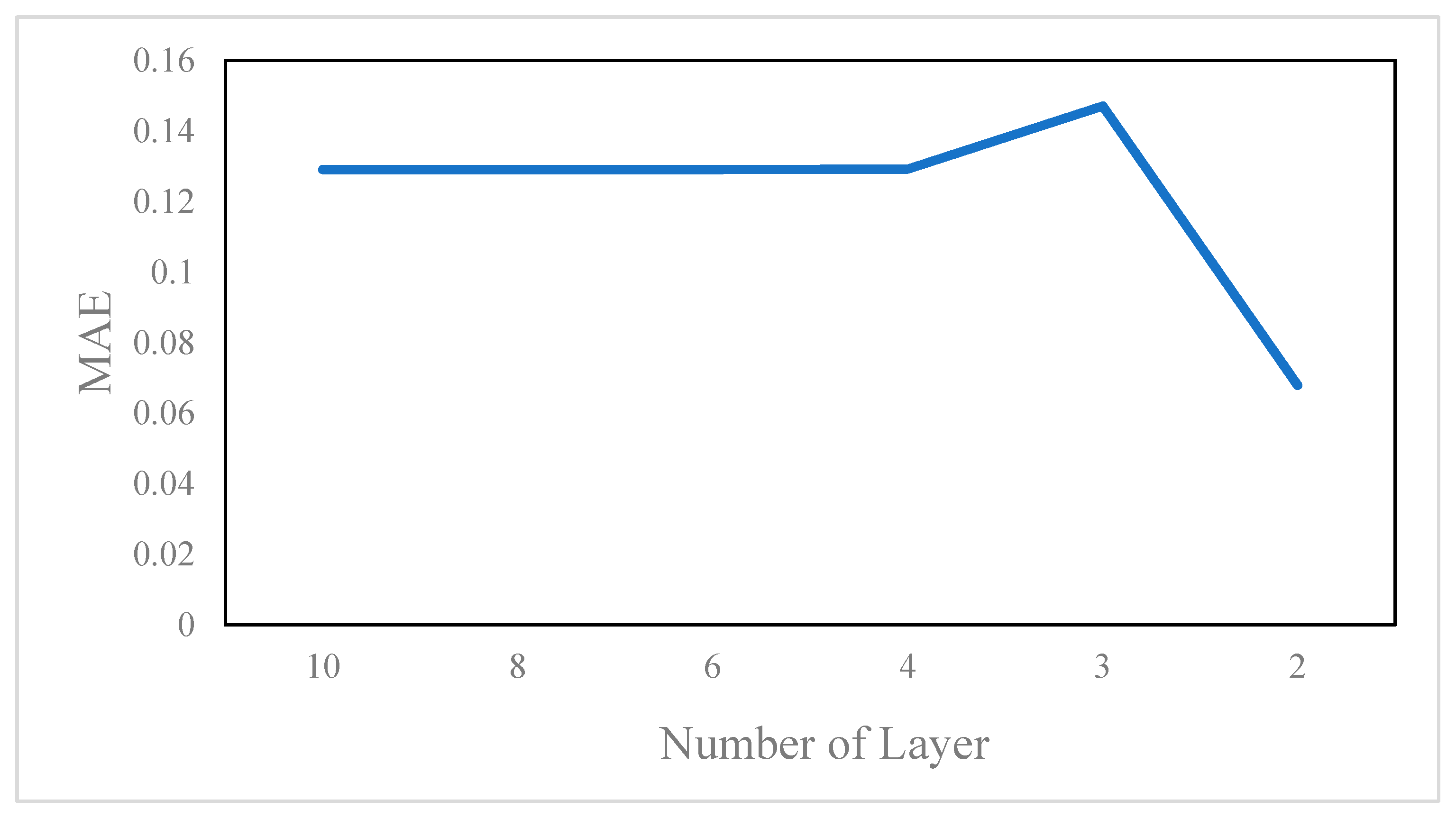
3.1.2. Number of RBM Layer

Six different numbers (10, 8, 6, 4, 3, 2) of RBM layers (Figure 5) were tested with a sample size of 3000. Other initial parameters were the same as previous experiments. Figure 3 shows that the DBN model of two RBM layers performs better (MAE of 0.06; visible node: 14; hidden node: 12). MAE rises quickly and reaches a peak of 0.15 when the RBM layer size is 3. MAEs have similar values around 0.13 when there are 3–10 RBM layers.

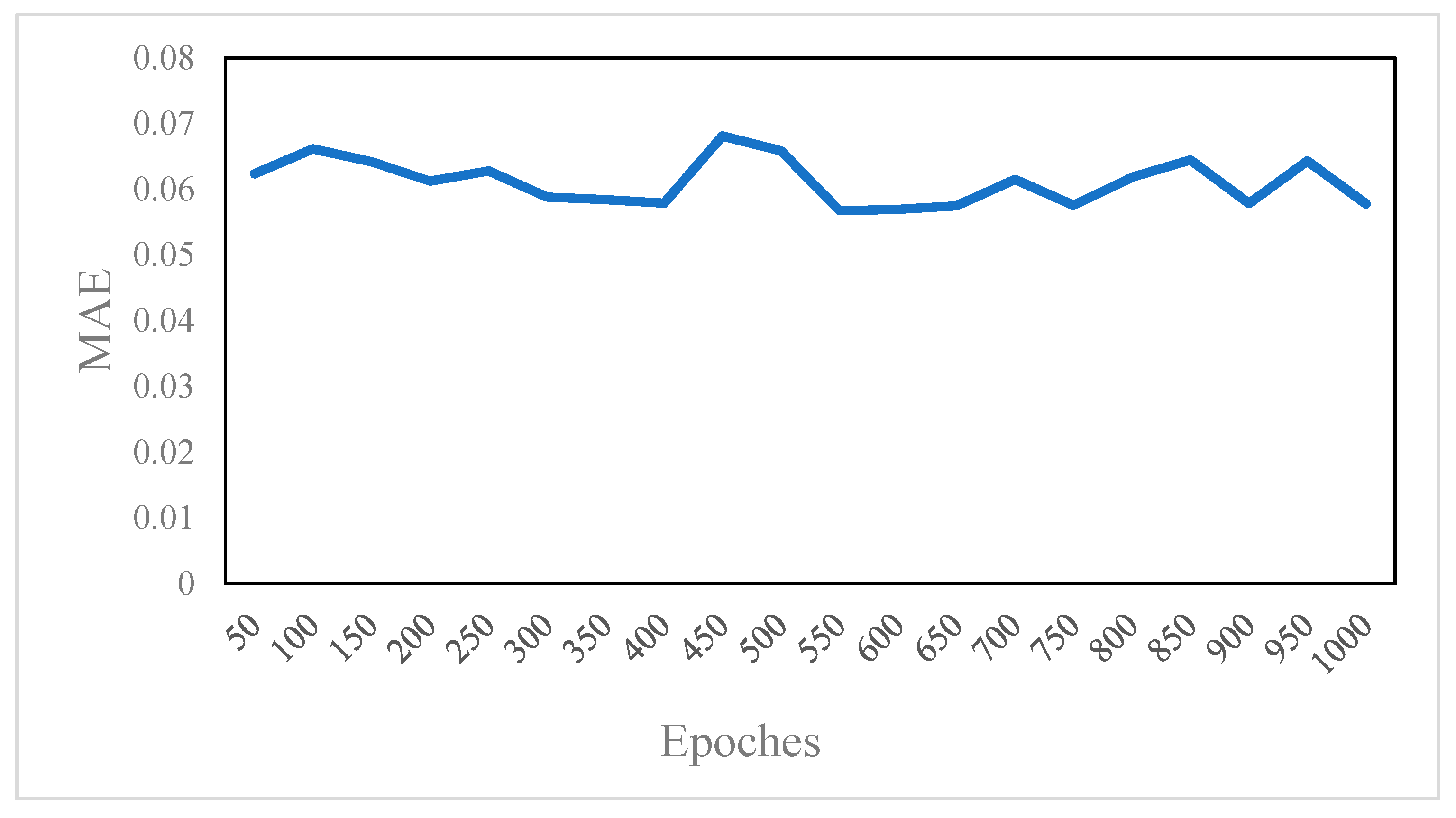
3.1.3. Number of Epochs

We tested the number of epochs from 50 to 1000 at an interval of 50. The sample size is 3000 and the number of RBM layers is 2. Other initial parameters were the same as previous experiments. MAEs are similar since they vary in a small range between 0.06 and 0.07 (Figure 6). This trend is not followed when the epochs increase from 50 to 1000.

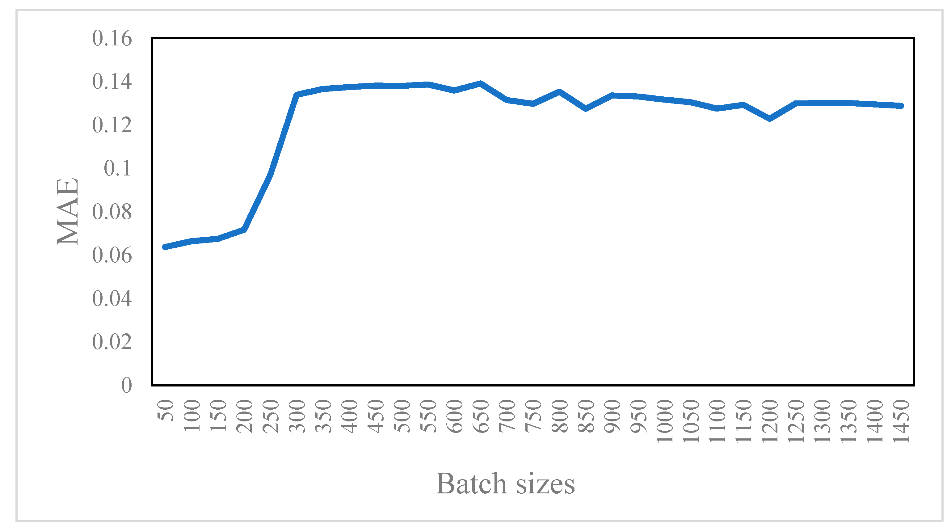
3.1.4. Number of Batch Size

The batch sizes were tested between 50 and 1450 with 150 epochs, 2 RBM layers, 3000 training samples and 0.1 learning rate. The results illustrate that MAEs increase slowly (from 0.06 to 0.07) when the batch size is between 50 and 200 (Figure 7). After this, MAEs increase dramatically from 0.07 to 0.13 when the range of batch sizes is 200–300. Finally, MAEs drop gradually from 0.136 to 0.128 when the batch size increases from 300 to 1450.

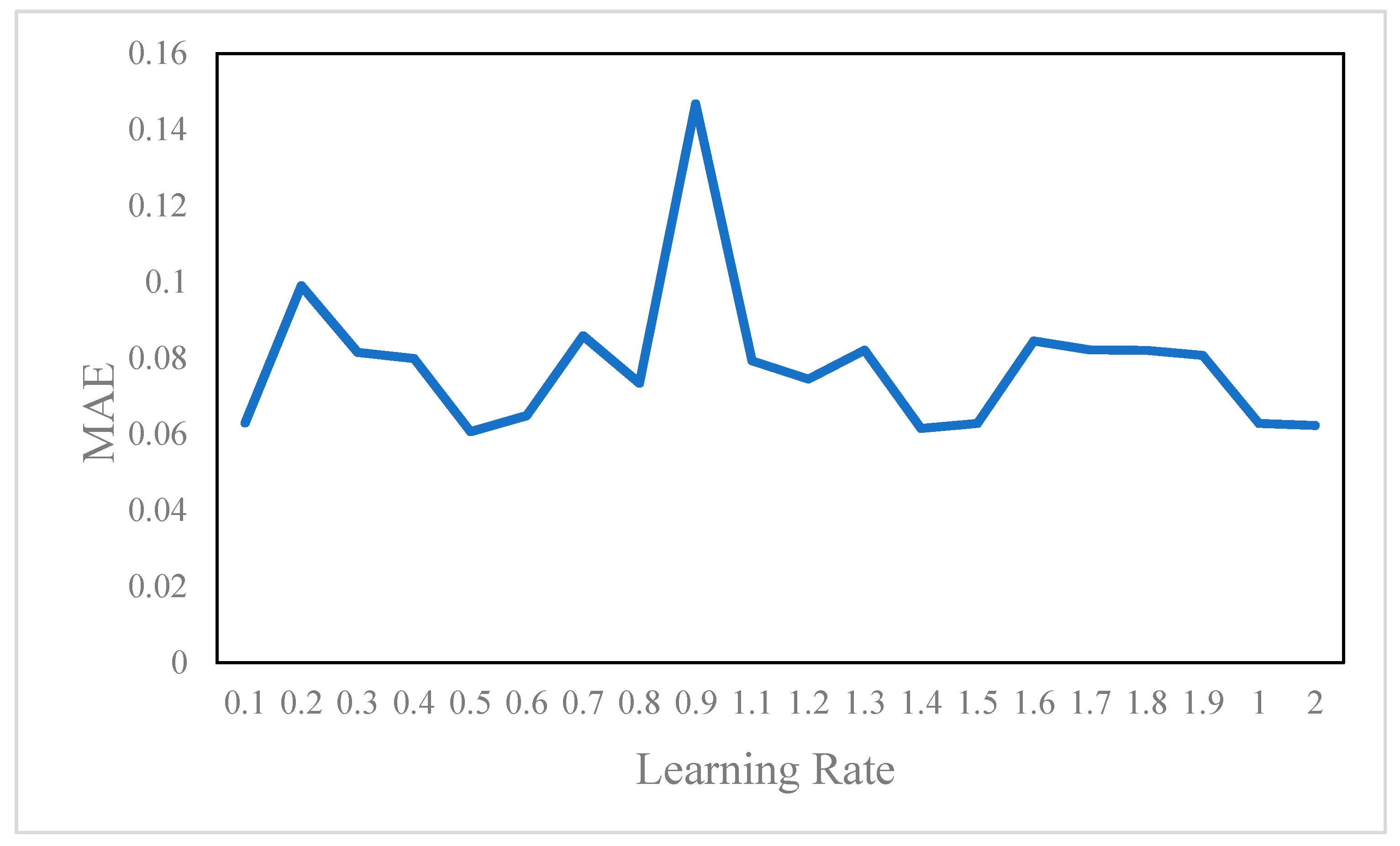
3.1.5. Learning Rate

We also tested learning rates of 0.1–2 (interval of 0.1) with a sample size of 3000, epoch of 50, batch size of 150 and 2 RBM layers. It seems that there is no consistent pattern for the changes in MAEs with an increase in the learning rates (Figure 8). MAEs vibrate dramatically from 0.146 to 0.06 with no significant trend. MAE reaches a peak of 0.15 at a learning rate of 0.9. The MAEs of other learning rates vary from 0.06 to 0.1 without any consistent pattern.

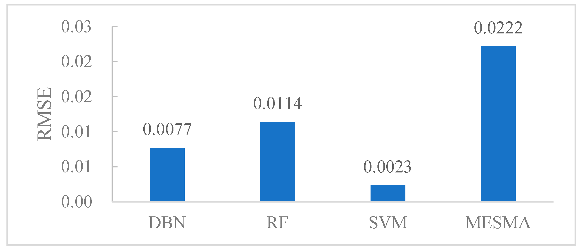
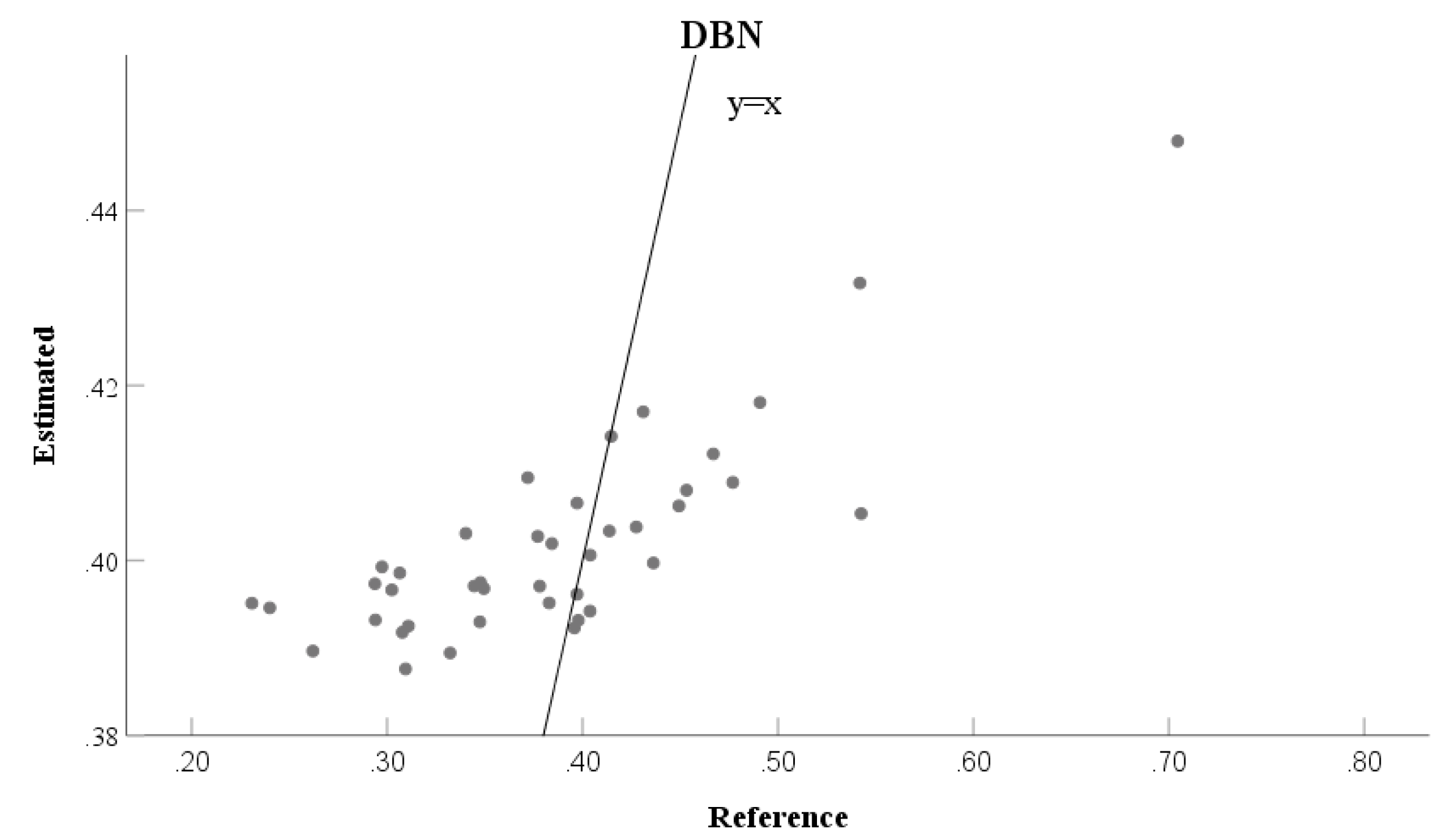
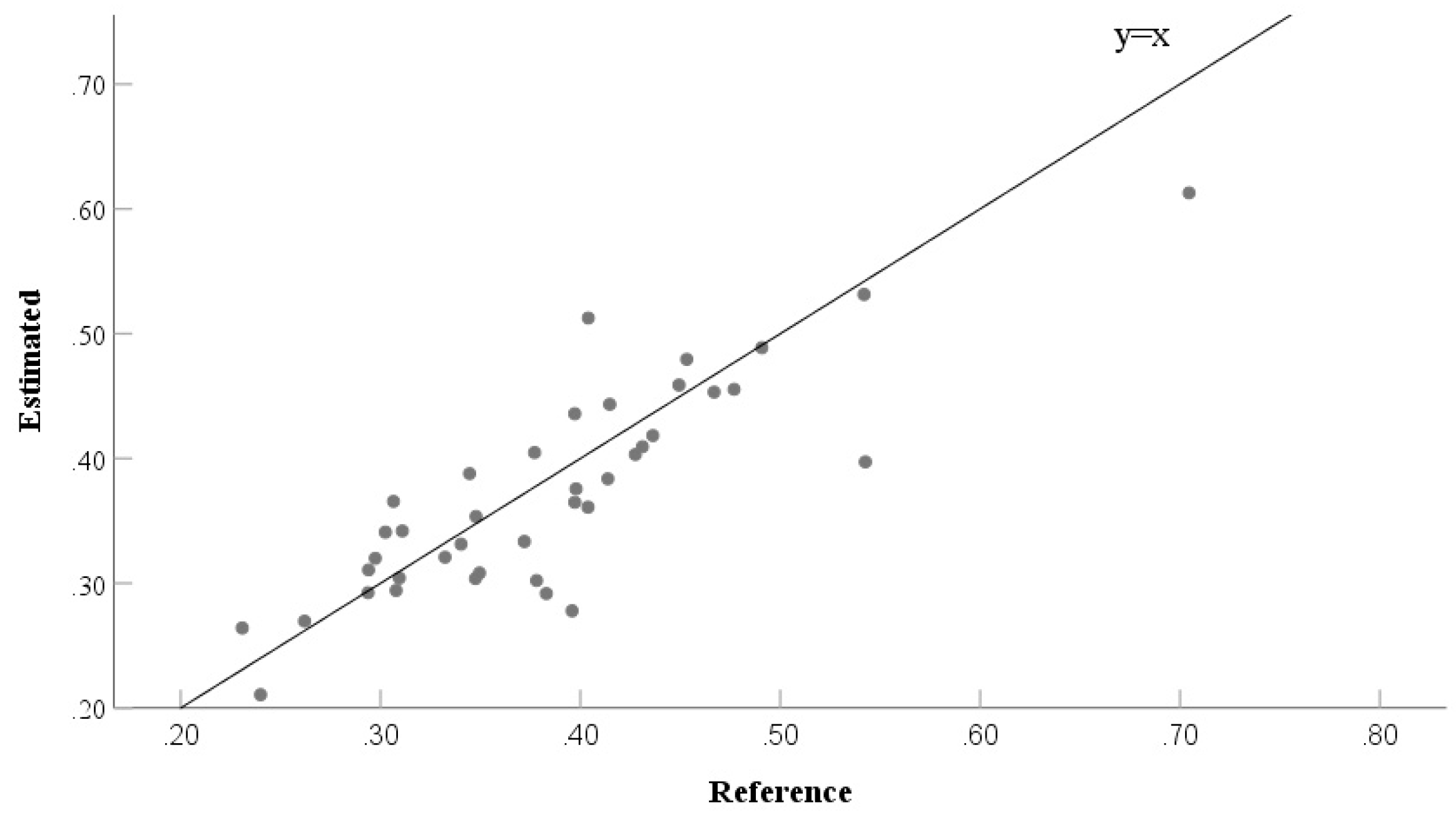
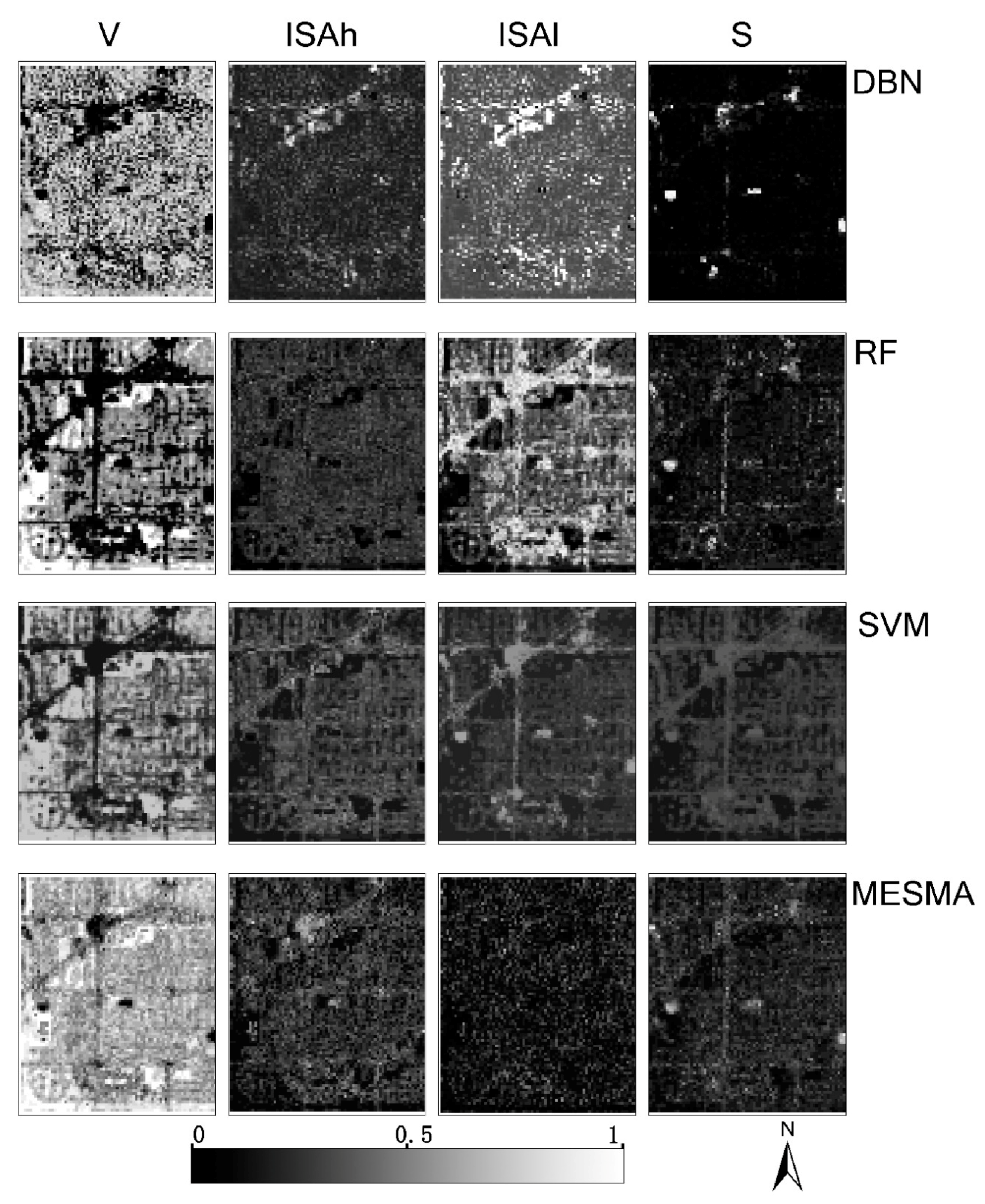
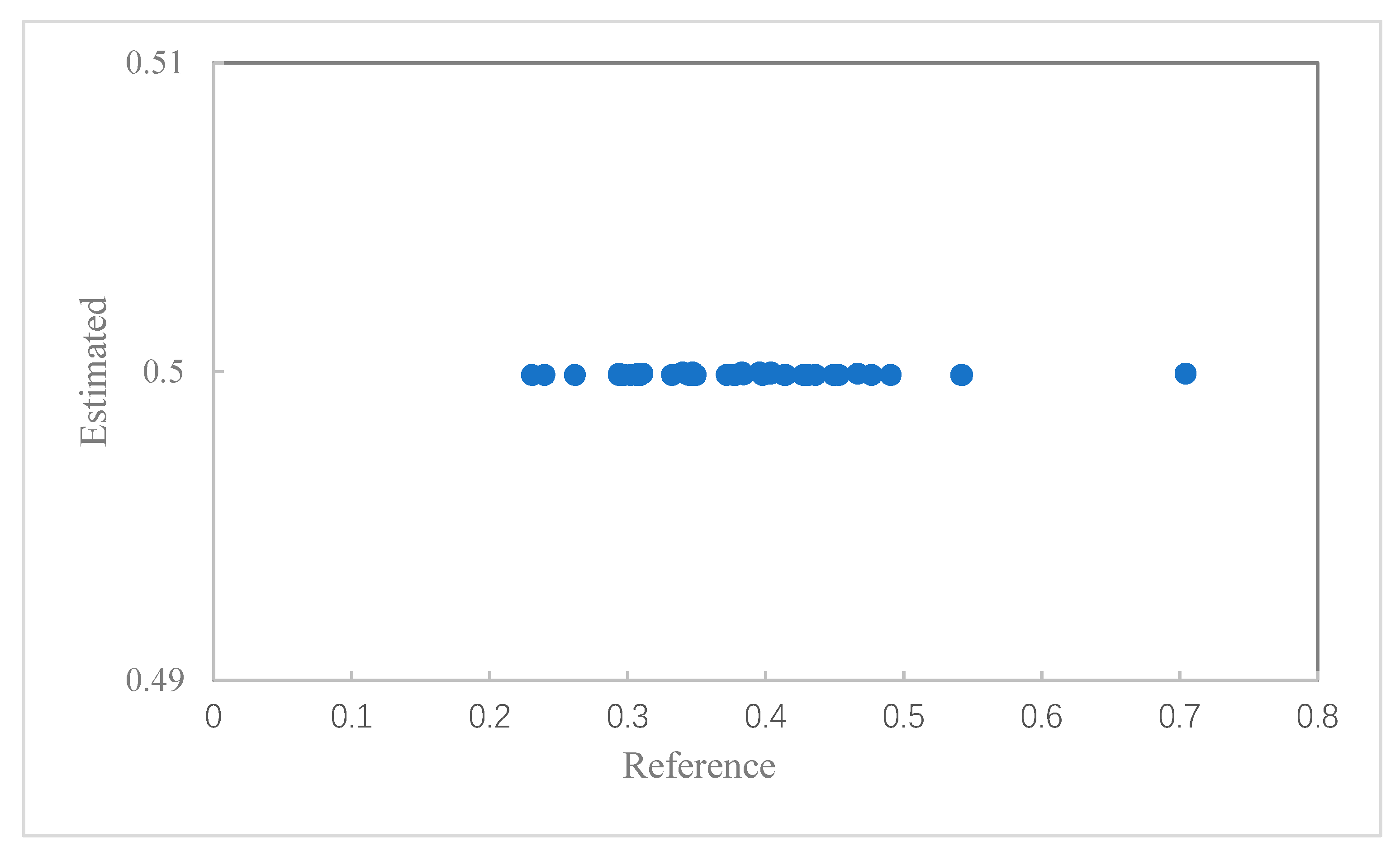
3.2. Accuracy Assessment and Comparative Analysis

In order to evaluate the performance of DBN more objectively, we compared the DBN with random forest (RF), support vector machine (SVM) and multiple endmember spectral mixture analysis (MESMA). We used 3000, 100, 5 and 10 samples (each class) for DBN, RF, SVM and MESMA, respectively. Histogram and scatter plots were employed for the numeric and visual comparisons. Histograms of MAE and RMSE illustrate that the best DBN (MAE: 0.06, RMSE: 0.0077) outperforms the best RF (MAE: 0.08, RMSE: 0.0114) and MESMA (MAE: 0.14, RMSE: 0.0222) while the SVM achieved the highest accuracy with a MAE of 0.03 and a RMSE of 0.0023 (Figure 9 and Figure 10).
Moreover, we also compared the time consumption of each model. The total number of pixels in the study area is 6192 with 86 rows and 72 columns. We used the Dell Precision Tower 7920 workstation with CPU of XEON Gold 5122 (4 Cores, 3.6 GHz), memory of 128 GB RDIMM and graphics card of NVIDIA Quadro P2000 (5 GB) for calculation. The results (Table 1) demonstrate that SVM can effectively predict the results within a second. DBN needs about 5 more minutes (310.89 s) to complete the calculation while RF needs more than 10 min to finish the unmixing process. Since there are 104 + 4 × 10³ + 6 × 10² endmember combinations (10 spectra for each class) in a pixel in the MESMA model, its calculation efficiency is very poor. MESMA takes about 25 days to finish the fraction estimate for 6192 pixels.
Scatterplots of estimated probabilities and referenced fractions were employed to demonstrate the detailed accuracy of each testing sample. Figure 11 shows that the reference line is almost located in the center of the scattered points, meaning that the percentages of overestimate and underestimate are similar. Figure 11 also illustrates that DBN underestimates the high ISA fraction testing samples while it overestimates the low ISA fraction samples. RF has a scatterplot pattern similar to that of DBN (Figure 12). The scatter points in SVM are almost located along with the referenced line of y = x, implying perfect matches between estimated probabilities and referenced fractions (Figure 13). All the fractions calculated in MESMA are underestimated since all scatter points are located on the right side of the referenced line (Figure 14).
In addition to MAE, RMSE and scatterplots, we also added visual comparisons of DBN, RF, SVM and MESMA (Figure 15). Figure 15 illustrates that RF and SVM can present the distinct road shapes in V (dark shape) and ISAl (light shape) fractional maps, while DBN and MESMA have poor performance in representing the shape of roads in all fraction maps. With the vegetation fraction maps, high vegetation fractions/possibilities are shown in grassland areas (see Figure 1) in the results of RF and MESMA. Compared to RF and MESMA, vegetation fractions/possibilities are relatively low in the grass land areas in the outputs from DBN and SVM. Most areas of RF, SVM and MESMA have low values in ISAh. DBN’s ISAh has medium values in dense built-up areas (see Figure 1), while it has low values in other areas. In ISAl fraction maps, the dense built-up areas have very high values in the results from DBN, while opposite results are obtained using MESMA. In the ISAl fraction maps of RF and SVM, high and medium values are located along the dense built-up areas and major roads. Further, DBN, RF and MESMA have significantly overestimated soil fractions in urban areas. The soil fractional values estimated by DBN are significantly higher compared to those estimated by RF and MESMA. Soil fractions estimated by SVM are low in the whole map but there are still some overestimations in urban areas.

4. Discussion

Currently, the applications of deep learning in remote sensing classification mainly focus on (1) pixel-based classification with hyperspectral imageries and (2) scene-based classification with high/very high spatial resolution aerial or satellite imageries. Few studies have utilized deep learning techniques to unmix medium spatial resolution multispectral imagery. Thus, this study examined the DBN model to unmix the mixed pixels in suburban areas with Landsat imagery. The results of DBN are not deterministic endmember fractions for a pixel, but probability distributions of each land cover classes.

4.1. Application of DBN in Landsat Imagery

Landsat series data only have six to seven available multispectral channels for classification. On the one hand, it can mitigate a large amount of data, which is one of the major challenges in remote sensing classification [20]. On the other hand, these limited bands also cause trouble in classification with deep learning techniques as limited wavebands provide a smaller amount of information. It is a challenge for deep learning techniques, such as DBN, to learn the comprehensive characteristics of each land cover class with these limited bands and this thus affects deep learning models’ performances. Sample size and model parameters are essential in successfully applying a DBN model with multispectral images. However, labeled training samples are another challenge in medium spatial resolution imagery [20]. Acquiring a large amount of labeled training samples in urban and suburban areas is impossible in medium spatial resolution images as a pixel’s corresponding ground area is larger than most independent objects on the ground. Therefore, mixed pixels, which contain more than one land cover type in a pixel, are inevitable. It is difficult to use mixed pixels as training samples in DBN because of the limitation of referenced fraction data. Thus, it is more difficult to apply DBN in medium spatial resolution multispectral imagery. To address the training sample limitation, we tried to collect training samples both from high spatial resolution hyperspectral imageries and from Landsat imagery themselves. The results demonstrated that these training samples can be utilized for the DBN and other machine learning methods. This may provide an alternative way for applications of deep learning in the collection of training samples when they are applied in medium spatial resolution multispectral imagery.

4.2. Application of DBN in Subpixel Unmixing

Similar to other machine learning based unmixing methods, DBN highlights the probabilities of spectral signatures while MESMA assumes equal probabilities for all endmembers [43]. After learning the characteristics of each land cover class, DBN estimates the probabilities of corresponding land cover types. Although other researchers have discussed using the endmember possibilities to replace endmember fractions in subpixel unmixing [40,44,45], a few studies applied deep learning techniques, especially the deep belief network, to estimate land covers’ probabilities. The results from this study illustrates that the probabilities estimated from DBN model are close to the land cover fractions in subpixel unmixing. Thus, it is appropriate to use probabilities calculated from DBN to estimate land cover fraction in a mixed pixel.
Parameter setting is an important step to achieve successful unmixing results. The experiments of this study have provided information on selecting a suitable sample size, number of RBM layers and batch size by iteratively comparing MAEs with different parameter values. Accuracy assessments imply that the experiments with larger sample sizes have higher accuracies, which matches the common assumption of deep learning techniques [30]. However, we also recognized that at least 3000 samples are necessary for DBN in subpixel unmixing with Landsat imagery. DBN with a sample size larger than 3000 has stable performance. On the contrary, MAE vibrated dramatically when the sample size is less than 1000. This may be first due to training sample subset selection. In this study, we reordered the training samples according to the sum of the band reflectance. After this, the samples were selected with a fixed interval. A smaller sample size results in a larger interval. Thus, the within-class variability in the training samples will be larger with a small sample size. Second, when the sample size is small, fewer characteristics can be provided. Therefore, DBN cannot learn about the comprehensive characteristics of each land cover class, leading to the vibration of model performance. When the sample size is larger than 3000, the major characteristics of all four training samples are shown in the selected subsets and this results in a smaller change. Therefore, the model performance becomes more stable.
In terms of the size of RBM layer, it seems that there is no more space for adjustments of RBM layer sizes since there are big differences between two-layer and more than two-layer MAEs. This may be due to the limited input wavebands in multispectral imagery. Compared to the experiment from reference [30] that which applied 30- or 50-layers for RBM, the number of RBM layer used in the study is very small. However, reference [30] implemented the DBN on hyperspectral data, which have hundreds of channels. Although the number of RBM layers in DBN, also known as the depth, is important for classification accuracy, the setting of depth may be affected by the number of channels in the data set. Thus, it makes sense for the two-RBM-layer model to have higher accuracy in this study.
The number of epochs (150) in this study is much less than the 1000–500 epochs from reference [30]. However, we cannot determine a consistent pattern for choosing the best-fit epochs since their MAEs are quite similar in all tests. The results from [46] also illustrated a similar result as there was no significant trend of accuracy when the epochs change from 50 to 200. However, our results match the conclusions of [47] as they illustrated that when the epoch size is larger than 15, the accuracy becomes stable.
The setting of the learning rate affects the rate of DBN learning. There is no a significant correlation between learning rates and MAEs. It seems that a lower rate does not mean higher accuracy. Reference [46] demonstrated similar results as the accuracy vibrated slightly when the learning rate changed from 0.2 to 0.7. A lower learning rate will theoretically lead to more reliable results. Time consumption will increase accordingly. However, this pattern did not occur in this study and in reference [46]. Other studies [23,47,48] have all used the same learning rate of 0.1 for their applications.
We tested a batch size of 50–1450. The results demonstrated that a smaller batch size results in better performance of the model. Generally, many studies only apply a batch size range of 50–150 [24,47,48]. Their results illustrated that a batch size selected within this range could have promising results.

4.3. Comparisons with Other Models

In the comparisons between SVM [40,44,49], RF [50] and MESMA [36], DBN [21]’s performance is close to SVM and RF. However, DBN requires significantly training samples than the other two techniques. That may be the reason for the lack of discussion of DBN in subpixel unmixing. Besides, DBN, similar to spectral mixture analysis [1], still cannot address the between-class variability since soil fractions are overestimated in dense built-up areas. However, its performance is higher than the MESMA and the calculational efficiency is better than MESMA in this study. Thus, DBN still can be viewed as an alternative method for subpixel unmixing in urban/suburban areas.
Soil fractions in DBN, SVM and MESMA are overestimated (Figure 15, column S). It may be due to the process of collecting soil samples. Most soil samples were collected from bare soil and sandy areas, such as beaches. These soil spectra are similar with those from high albedo impervious surface areas [51,52]. It is easy to mistaken them for high albedo impervious surface areas in classification [53]. The results in this study provide references about different models’ capabilities of distinguishing soil and high albedo impervious surface areas. SVM [44] is the best model to identify soil and impervious surfaces even though the training samples are limited.
In addition, we also tested the models of deep autoencoder network (DAEN) [54,55] and pixel-based Convolutional Neural Networks (CNN) [10,16,56]. However, their performances are inferior to that of DBN (Figure 16 and Figure 17). With the DAEN model, we have tested it with different sample sizes, learning rates, steps, batch sizes, regularizers and moving average decays. Their results are similar to Figure 16, which shows that the ISA possibilities are almost the same in different testing experiments.
Similar to DAEN, we tested pixel-based CNN [10,16,56] with different parameters, such as testing sample sizes of 100–500, batch sizes of 50–500 and learning rates of 0.001–0.2. However, the probabilistic maps are similar to Figure 17. Figure 17 illustrates the inaccurate probability distributions of vegetation.
Figure 16 and Figure 17 imply that DAEN and CNN may perform well in hyperspectral imagery [10,16,54,55,56] but not in medium spatial resolution multispectral imagery. The number of channels is the major difference between multispectral and hyperspectral imageries. Experiments of DAEN and CNN demonstrate that the number of channels is a key parameter determining their successful applications. Therefore, we did not add these two models for comparison in this study.

5. Conclusions

This study examined the DBN model in subpixel unmixing with Landsat imagery. The results illustrated that the DBN model can perform well in subpixel unmixing. Different tests were performed to determine the best-fit parameters in DBN model. Several conclusions can be achieved. (1) DBN can provide comparable results to RF, SVM and MESMA in medium spatial resolution multispectral imagery. (2) A larger training sample size, especially larger than 3000, can acquire better and more stable results in DBN while two RBM layers and a batch size of 50 is better for Landsat imagery since it has the lowest MAE. (3) The setting of the learning rate and epoch should be based on specific applications since there is no consistent pattern in our experiments. The major contribution of this study is the examination of the applicability of DBN in subpixel unmixing with Landsat imagery. The results of this research may serve as references for scholars to explore the use of DBN in subpixel unmixing with medium spatial resolution multispectral imagery.

Author Contributions

Conceptualization, Y.D. and R.C.; methodology, Y.D.; writing—original draft preparation, Y.D. and R.C.; writing—review and editing, C.W.

Funding

This research was funded by GDAS Project of Science and Technology Development, China (2019GDASYL-0103004, 2016GDASRC-0211, 2018GDASCX-0403, 2019GDASYL-0301001, 2019GDASYL-0501001), Guangdong Innovative and Entrepreneurial Research Team Program (2016ZT06D336) and The APC was funded by GDAS Project of Science and Technology Development, China (2019GDASYL-0103004).

Acknowledgments

The authors would like to thank the anonymous reviewers for their constructive comments. We also want to thank Yichun Xie and Xinyue Ye for providing constructive suggestions about this study.

Conflicts of Interest

The authors declare no conflict of interest.

References

  1. Adams, J.B.; Smith, M.O.; Johnson, P.E. Spectral mixture modeling: A new analysis of rock and soil types at the Viking Lander 1 site. J. Geophys. Res. Solid Earth 1986, 91, 8098–8112. [Google Scholar] [CrossRef]
  2. Horwitz, H.M.; Nalepka, R.F.; Hyde, P.D.; Morgenstern, J.P. Estimating the Proportions of Objects within a Single Resolution Element of a Multispectral Scanner; NASA Contract NAS-9-9784; University of Michigan: Ann Arbor, MI, USA, 1971. [Google Scholar]
  3. Marsh, S.E.; Switzer, P.; Kowalik, W.S.; Lyon, R.J. Resolving the percentage of component terrains within single resolution elements. Photogramm. Eng. Remote Sens. 1980, 46, 1079–1086. [Google Scholar]
  4. Li, X.; Strahler, A.H. Geometric-optical modeling of a conifer forest canopy. IEEE Trans. Geosci. Remote Sens. 1985, GE-23, 705–721. [Google Scholar] [CrossRef]
  5. Strahler, A.; Woodcock, C.; Xiaowen, L.; Jupp, D. Discrete-Object Modeling of Remotely Sensed Scenes. In Proceedings of the 18th International Symposium on Remote Sensing of Environment, Paris, France, 1–5 October 1984; Environmental Research Institute of Michigan: Ann Arbor, MI, USA, 1985; Volume 1, pp. 465–473. [Google Scholar]
  6. Jasinski, M.F.; Eagleson, P.S. The structure of red-infrared scattergrams of semivegetated landscapes. IEEE Trans. Geosci. Remote Sens. 1989, 27, 441–451. [Google Scholar] [CrossRef]
  7. Jasinski, M.F.; Eagleson, P.S. Estimation of subpixel vegetation cover using red-infrared scattergrams. IEEE Trans. Geosci. Remote Sens. 1990, 28, 253–267. [Google Scholar] [CrossRef]
  8. Kent, J.T.; Mardia, K.V. Spatial classification using fuzzy membership models. IEEE Trans. Pattern Anal. Mach. Intell. 1988, 10, 659–671. [Google Scholar] [CrossRef]
  9. Foody, G. A fuzzy sets approach to the representation of vegetation continua from remotely sensed data: An example from lowland heath. Photogramm. Eng. Remote Sens. 1992, 58, 221–225. [Google Scholar]
  10. Arun, P.; Buddhiraju, K.M.; Porwal, A. CNN based sub-pixel mapping for hyperspectral images. Neurocomputing 2018, 311, 51–64. [Google Scholar] [CrossRef]
  11. Liu, Q.; Zhou, F.; Hang, R.; Yuan, X. Bidirectional-convolutional LSTM based spectral-spatial feature learning for hyperspectral image classification. Remote Sens. 2017, 9, 1330. [Google Scholar]
  12. Mou, L.; Ghamisi, P.; Zhu, X.X. Deep recurrent neural networks for hyperspectral image classification. IEEE Trans. Geosci. Remote Sens. 2017, 55, 3639–3655. [Google Scholar] [CrossRef]
  13. Chaurasia, A.; Culurciello, E. Linknet: Exploiting encoder representations for efficient semantic segmentation. In Proceedings of the 2017 IEEE Visual Communications and Image Processing (VCIP), St. Petersburg, Russia, 10–13 December 2017; pp. 1–4. [Google Scholar]
  14. Ji, S.; Xu, W.; Yang, M.; Yu, K. 3D convolutional neural networks for human action recognition. IEEE Trans. Pattern Anal. Mach. Intell. 2012, 35, 221–231. [Google Scholar] [CrossRef] [PubMed]
  15. Ling, F.; Foody, G.M. Super-resolution land cover mapping by deep learning. Remote Sens. Lett. 2019, 10, 598–606. [Google Scholar] [CrossRef]
  16. Zhao, S.; Zhang, L.; Shen, Y.; Zhu, Y. A CNN-Based Depth Estimation Approach with Multi-scale Sub-pixel Convolutions and a Smoothness Constraint. In Proceedings of the 14th Asian Conference on Computer Vision, Perth, Australia, 2–6 December 2018; pp. 365–380. [Google Scholar]
  17. Arun, P.; Buddhiraju, K.M. A deep learning based spatial dependency modelling approach towards super-resolution. In Proceedings of the 2016 IEEE International Geoscience and Remote Sensing Symposium (IGARSS), Beijing, China, 10–15 July 2016; pp. 6533–6536. [Google Scholar]
  18. Guo, R.; Wang, W.; Qi, H. Hyperspectral image unmixing using autoencoder cascade. In Proceedings of the 2015 7th Workshop on Hyperspectral Image and Signal Processing: Evolution in Remote Sensing (WHISPERS), Tokyo, Japan, 2–5 June 2015; pp. 1–4. [Google Scholar]
  19. Ma, A.; Zhong, Y.; He, D.; Zhang, L. Multiobjective subpixel land-cover mapping. IEEE Trans. Geosci. Remote Sens. 2018, 56, 422–435. [Google Scholar] [CrossRef]
  20. Li, Y.; Zhang, H.; Xue, X.; Jiang, Y.; Shen, Q. Deep learning for remote sensing image classification: A survey. Wiley Interdiscip. Rev. Data Min. Knowl. Discov. 2018, 8, e1264. [Google Scholar] [CrossRef]
  21. Hinton, G.E.; Osindero, S.; Teh, Y.-W. A fast learning algorithm for deep belief nets. Neural Comput. 2006, 18, 1527–1554. [Google Scholar] [CrossRef] [PubMed]
  22. Lv, Q.; Dou, Y.; Niu, X.; Xu, J.; Xu, J.; Xia, F. Urban land use and land cover classification using remotely sensed SAR data through deep belief networks. J. Sens. 2015, 2015, 538063. [Google Scholar] [CrossRef]
  23. Zhong, P.; Gong, Z.; Li, S.; Schönlieb, C.-B. Learning to diversify deep belief networks for hyperspectral image classification. IEEE Trans. Geosci. Remote Sens. 2017, 55, 3516–3530. [Google Scholar] [CrossRef]
  24. Diao, W.; Sun, X.; Zheng, X.; Dou, F.; Wang, H.; Fu, K. Efficient saliency-based object detection in remote sensing images using deep belief networks. IEEE Geosci. Remote Sens. Lett. 2016, 13, 137–141. [Google Scholar] [CrossRef]
  25. Diao, W.; Sun, X.; Dou, F.; Yan, M.; Wang, H.; Fu, K. Object recognition in remote sensing images using sparse deep belief networks. Remote Sens. Lett. 2015, 6, 745–754. [Google Scholar] [CrossRef]
  26. Nakashika, T.; Takiguchi, T.; Ariki, Y. High-frequency restoration using deep belief nets for super-resolution. In Proceedings of the 2013 International Conference on Signal-Image Technology & Internet-Based Systems, Kyoto, Japan, 2–5 December 2013; pp. 38–42. [Google Scholar]
  27. Burges, C.J. A tutorial on support vector machines for pattern recognition. Data Min. Knowl. Discov. 1998, 2, 121–167. [Google Scholar] [CrossRef]
  28. Hu, W.; Huang, Y.; Wei, L.; Zhang, F.; Li, H. Deep convolutional neural networks for hyperspectral image classification. J. Sens. 2015, 2015, 258619. [Google Scholar] [CrossRef]
  29. Moser, G.; Zerubia, J.; Serpico, S.B. Dictionary-based stochastic expectation-maximization for SAR amplitude probability density function estimation. IEEE Trans. Geosci. Remote Sens. 2005, 44, 188–200. [Google Scholar] [CrossRef] [Green Version]
  30. Chen, Y.; Zhao, X.; Jia, X. Spectral–spatial classification of hyperspectral data based on deep belief network. IEEE J. Sel. Top. Appl. Earth Obs. Remote Sens. 2015, 8, 2381–2392. [Google Scholar] [CrossRef]
  31. Ayhan, B.; Kwan, C. Application of deep belief network to land cover classification using hyperspectral images. In Advances in Neural Networks—ISNN 2017; Cong, F., Leung, A., Wei, Q., Eds.; Lecture Notes in Computer Science; Springer: Cham, Switzerland, 2017; Volume 10261, pp. 269–276. [Google Scholar]
  32. Mughees, A.; Tao, L. Multiple deep-belief-network-based spectral-spatial classification of hyperspectral images. Tsinghua Sci. Technol. 2019, 24, 183–194. [Google Scholar] [CrossRef]
  33. Zou, Q.; Ni, L.; Zhang, T.; Wang, Q. Deep learning based feature selection for remote sensing scene classification. IEEE Geosci. Remote Sens. Lett. 2015, 12, 2321–2325. [Google Scholar] [CrossRef]
  34. Sowmya, V.; Ajay, A.; Govind, D.; Soman, K. Improved color scene classification system using deep belief networks and support vector machines. In Proceedings of the 2017 IEEE International Conference on Signal and Image Processing Applications (ICSIPA), Kuching, Malaysia, 12–14 September 2017; pp. 33–38. [Google Scholar]
  35. Ma, L.; Liu, Y.; Zhang, X.; Ye, Y.; Yin, G.; Johnson, B.A. Deep learning in remote sensing applications: A meta-analysis and review. ISPRS J. Photogramm. Remote Sens. 2019, 152, 166–177. [Google Scholar] [CrossRef]
  36. Roberts, D.A.; Gardner, M.; Church, R.; Ustin, S.; Scheer, G.; Green, R. Mapping chaparral in the Santa Monica Mountains using multiple endmember spectral mixture models. Remote Sens Environ. 1998, 65, 267–279. [Google Scholar] [CrossRef]
  37. Reschke, J.; Hüttich, C. Continuous field mapping of Mediterranean wetlands using sub-pixel spectral signatures and multi-temporal Landsat data. Int. J. Appl. Earth Obs. Geoinf. 2014, 28, 220–229. [Google Scholar] [CrossRef]
  38. Tsutsumida, N.; Comber, A.; Barrett, K.; Saizen, I.; Rustiadi, E. Sub-pixel classification of MODIS EVI for annual mappings of impervious surface areas. Remote Sens. 2016, 8, 143. [Google Scholar] [CrossRef]
  39. Breiman, L. Random forests. Mach. Learn. 2001, 45, 5–32. [Google Scholar] [CrossRef]
  40. Bovolo, F.; Bruzzone, L.; Carlin, L. A novel technique for subpixel image classification based on support vector machine. IEEE Trans. Image Process. 2010, 19, 2983–2999. [Google Scholar] [CrossRef]
  41. Mountrakis, G.; Im, J.; Ogole, C. Support vector machines in remote sensing: A review. ISPRS J. Photogramm. Remote Sens. 2011, 66, 247–259. [Google Scholar] [CrossRef]
  42. Ridd, M.K. Exploring a VIS (vegetation-impervious surface-soil) model for urban ecosystem analysis through remote sensing: Comparative anatomy for cities†. Int. J. Remote Sens 1995, 16, 2165–2185. [Google Scholar] [CrossRef]
  43. Song, C. Spectral mixture analysis for subpixel vegetation fractions in the urban environment: How to incorporate endmember variability? Remote Sens Environ. 2005, 95, 248–263. [Google Scholar] [CrossRef]
  44. Brown, M.; Gunn, S.R.; Lewis, H.G. Support vector machines for optimal classification and spectral unmixing. Ecol. Model. 1999, 120, 167–179. [Google Scholar] [CrossRef]
  45. Huang, X.; Schneider, A.; Friedl, M.A. Mapping sub-pixel urban expansion in China using MODIS and DMSP/OLS nighttime lights. Remote Sens Environ. 2016, 175, 92–108. [Google Scholar] [CrossRef]
  46. Jiang, Z.; Ma, Y.; Jiang, T.; Chen, C. Research on the Extraction of Red Tide Hyperspectral Remote Sensing Based on the Deep Belief Network (DBN). J. Ocean. Technol. 2019, 38, 1–7. [Google Scholar]
  47. Xu, L.; Liu, X.; Xiang, X. Recognition and Classification for Remote Sensing Image Based on Depth Belief Network. Geol. Sci. Technol. Inf. 2017, 36, 244–249. [Google Scholar]
  48. Deng, L.; Fu, S.; Zhang, R. Application of deep belief network in polarimetric SAR image classification. J. Image Graph. 2016, 21, 933–941. [Google Scholar]
  49. Melgani, F.; Bruzzone, L. Classification of hyperspectral remote sensing images with support vector machines. Geosci. Remote Sens. IEEE Trans. 2004, 42, 1778–1790. [Google Scholar] [CrossRef] [Green Version]
  50. Pal, M. Random forest classifier for remote sensing classification. Int. J. Remote Sens. 2005, 26, 217–222. [Google Scholar] [CrossRef]
  51. Hu, X.; Weng, Q. Estimating impervious surfaces from medium spatial resolution imagery using the self-organizing map and multi-layer perceptron neural networks. Remote Sens. Environ. 2009, 113, 2089–2102. [Google Scholar] [CrossRef]
  52. Lu, D.; Weng, Q. Extraction of urban impervious surfaces from an IKONOS image. Int. J. Remote Sens. 2009, 30, 1297–1311. [Google Scholar] [CrossRef]
  53. Deng, Y.; Wu, C. Development of a Class-Based Multiple Endmember Spectral Mixture Analysis (C-MESMA) Approach for Analyzing Urban Environments. Remote Sens. 2016, 8, 349. [Google Scholar] [CrossRef]
  54. Su, Y.; Li, J.; Plaza, A.; Marinoni, A.; Gamba, P.; Chakravortty, S. DAEN: Deep Autoencoder Networks for Hyperspectral Unmixing. IEEE Trans. Geosci. Remote Sens. 2019, 57, 4309–4321. [Google Scholar] [CrossRef]
  55. Lin, Z.; Chen, Y.; Zhao, X.; Wang, G. Spectral-spatial classification of hyperspectral image using autoencoders. In Proceedings of the 2013 9th International Conference on Information, Communications & Signal Processing, Tainan, Taiwan, 10–13 December 2013; pp. 1–5. [Google Scholar]
  56. Zhang, X.; Sun, Y.; Zhang, J.; Wu, P.; Jiao, L. Hyperspectral Unmixing via Deep Convolutional Neural Networks. IEEE Geosci. Remote Sens. Lett. 2018, 15, 1755–1759. [Google Scholar] [CrossRef]
Figure 1. Suburban area in Milwaukee County, Wisconsin, United States. The study area is marked by the red rectangle.
Remotesensing 11 01566 g001
Figure 2. Hyperspectral image for training sample collection. (a) Original hyperspectral image; (b) Training samples in the hyperspectral image. For the training sample, Green: Vegetation (V); Red: High albedo impervious surface area (ISAh); Blue: Low albedo impervious surface area ISAl; and Yellow: soil/sand (S).
Remotesensing 11 01566 g002
Figure 3. Distribution of testing samples. The small red squares were the testing samples in our study areas.
Remotesensing 11 01566 g003
Figure 4. MAEs of different sample sizes.
Remotesensing 11 01566 g004
Figure 5. MAEs of different RBM layers.
Remotesensing 11 01566 g005
Figure 6. MAEs of different epochs.
Remotesensing 11 01566 g006
Figure 7. MAEs of different batch sizes.
Remotesensing 11 01566 g007
Figure 8. MAEs of different learning rates.
Remotesensing 11 01566 g008
Figure 9. MAEs of different models.
Remotesensing 11 01566 g009
Figure 10. RMSEs of different models.
Remotesensing 11 01566 g010
Figure 11. MAEs of DBN.
Remotesensing 11 01566 g011
Figure 12. MAEs of RF.
Remotesensing 11 01566 g012
Figure 13. MAEs of SVM.
Remotesensing 11 01566 g013
Figure 14. MAEs of MESMA.
Remotesensing 11 01566 g014
Figure 15. Visual comparisons between DBN, RF, SVM and MESMA. Column V represents vegetation, Column ISAh represents a high albedo impervious surface area, Column ISAl represents a low albedo impervious surface area and Column S represents soil.
Remotesensing 11 01566 g015
Figure 16. Scatterplot of ISA with DAEN model.
Remotesensing 11 01566 g016
Figure 17. Vegetation probabilistic map of CNN model with 3000 training samples.
Remotesensing 11 01566 g017
Table 1. Time consumption of different models.
DBNRFSVMMESMA
Samples for each class3000100510
Training Time (seconds)305.600.520.03/
Prediction Time (seconds)5.29637.60.332.16 × 106
Total Time (seconds)310.89638.120.362.16 × 106

