Technical Note

Crack Propagation and Fracture Process Zone (FPZ) of Wood in the Longitudinal Direction Determined Using Digital Image Correlation (DIC) Technique

1
Department of Civil Engineering, Shantou University, Shantou 515063, China
2
Department of Civil Engineering, Beijing Forestry University, Beijing 10083, China
3
College of Civil Engineering and Architecture, Zhejiang University, Hanghzou 310027, China
4
Department of Civil and Environmental Engineering, University of Wisconsin, Platteville, WI 53818, USA
*
Author to whom correspondence should be addressed.
Remote Sens. 2019, 11(13), 1562; https://doi.org/10.3390/rs11131562
Submission received: 6 May 2019 / Revised: 27 June 2019 / Accepted: 28 June 2019 / Published: 2 July 2019
(This article belongs to the Special Issue Vision-Based Sensing in Engineering Structures)

Abstract

:
As a state-of-the-art method, the digital image correlation (DIC) technique is used to capture the fracture properties of wood along the longitudinal direction, such as the crack propagation, the strain field, and the fracture process zone (FPZ). Single-edge notched (SEN) specimens made of Douglas fir (Pseudotsuga menziesii) from Canada with different notch-to-depth ratios are tested by three-point-bending (3-p-b) experiment. The crack mouth opening displacements (CMOD) measured by the clip gauge and DIC technique agree well with each other, verifying the applicability of the DIC technique. Then, the quasi-brittle fracture process of wood is analyzed by combing the load-CMOD curve and the strain field in front of the preformed crack. Additionally, the equivalent elastic crack length is calculated using the linear superposition hypothesis. The comparison between the FPZ evolution and the equivalent elastic crack shows that specimens with higher notch-to-depth ratios have better cohesive effect and higher cracking resistance.

1. Introduction

As a green and natural engineering material, wood has been widely used in construction. However, some inherent defects in wood produce stress concentrations and then cause failure cracks in the material when it is under tension and bending. Therefore, crack propagation in wood structures has gained much scientific and technological attention [1,2].
As a typical orthotropic material, wood has three directions of material symmetry: L (the longitudinal direction along the tree trunk), R (the radial direction of the annual rings), and T (the tangential direction to the annual rings). It is recognized that mode I fracture along the L direction is the most important failure mode in wood structures [3].
The fracture process zone (FPZ) is defined as the region ahead of the traction free crack tip [4]. This region contains lots of distribute microcracks, in which the mechanical behavior, such as stress transformation, are quite complicate. As a kind of quasi-brittle material, wood has FPZ in front of the crack tip [5]. The FPZ size (length and width) reflects the fracture properties, such as fracture toughness and fracture energy [6,7]. FPZ is also used in the analysis of boundary effect mode [8] and can be combined with the critical crack length to reveal the properties of the fracture [9]. Therefore, the identification of FPZ evolution is essential to explain wood fracture [10,11].
Until now, many direct methods have been used to determine the crack propagation and FPZ size of quasi-brittle fracture, such as acoustic emission (AE) method [12], laser holography method [13], speckle interferometry method [14], and a relatively new technique — digital image correlation (DIC) method. Compared with other direct methods in crack measurement, DIC method can obtain the specimen full-field incremental displacement with simple experiment preparation, as well as being insensitive to environmental noise for general cases [15]. It can obtain the surface displacement by tracking homologous points on the specimen surface at different loading processes. Furthermore, with high quality speckle digital images and a good correlation algorithm, DIC result is reliable and accurate [16].
Due to the aforementioned advantages, DIC has been widely used in recent fracture investigations due to its many advantages. For example, Yates et al. employed DIC method to quantify the crack tip displacement field and calculate the stress intensity factor [17]. Lin et al. determined the critical crack opening displacement and FPZ length of sandstone according to the displacement contour in front of the crack tip [18]. Dong et al. estimated the FPZ size of mixed mode fracture in concrete by tracking the horizontal displacement variation around the crack tip [19].
In accordance with the FPZ evolution, the crack propagation along the L direction is composed of two parts, which can be conceptually related to the micro-cracking and the crack-bridging phenomena [7], respectively. Due to the crack bridging phenomena, linear elastic fracture mechanics (LEFM) cannot be directly applied to quasi-brittle fractures in wood. A so-called ‘equivalent LEFM’ is usually adopted to provide valid approximations of fracture properties [2,3]. The equivalent elastic crack of length aeq is one of the fundamental parameters in equivalent LEFM. The tip of this equivalent linear elastic crack is not located at the beginning of the FPZ, but some distance Δa ahead: aeq = a0 + Δa, where a0 is the length of the preformed crack. Based on the equivalent LEFM, the fracture toughness and R curve of timber were calculated [20,21]. However, the relationship between FPZ and aeq are seldom analyzed during the fracture process.
In this study, the mode I fracture behavior of Douglas fir (Pseudotsuga menziesii) along the L direction was studied by three-point bending (3-p-b) test. It is found that wood, as a quasi-brittle material, has a three-stage fracture process, which is consistent with crack growth. The DIC technique is used to analyze the crack propagation, strain field and FPZ size. In addition, the evolution of FPZ is compared with the equivalent elastic crack as to illustrate the physical meaning of the two fracture parameters as well as to analyze the influence of notch-to-depth ratio on the fracture properties.

2. Methods

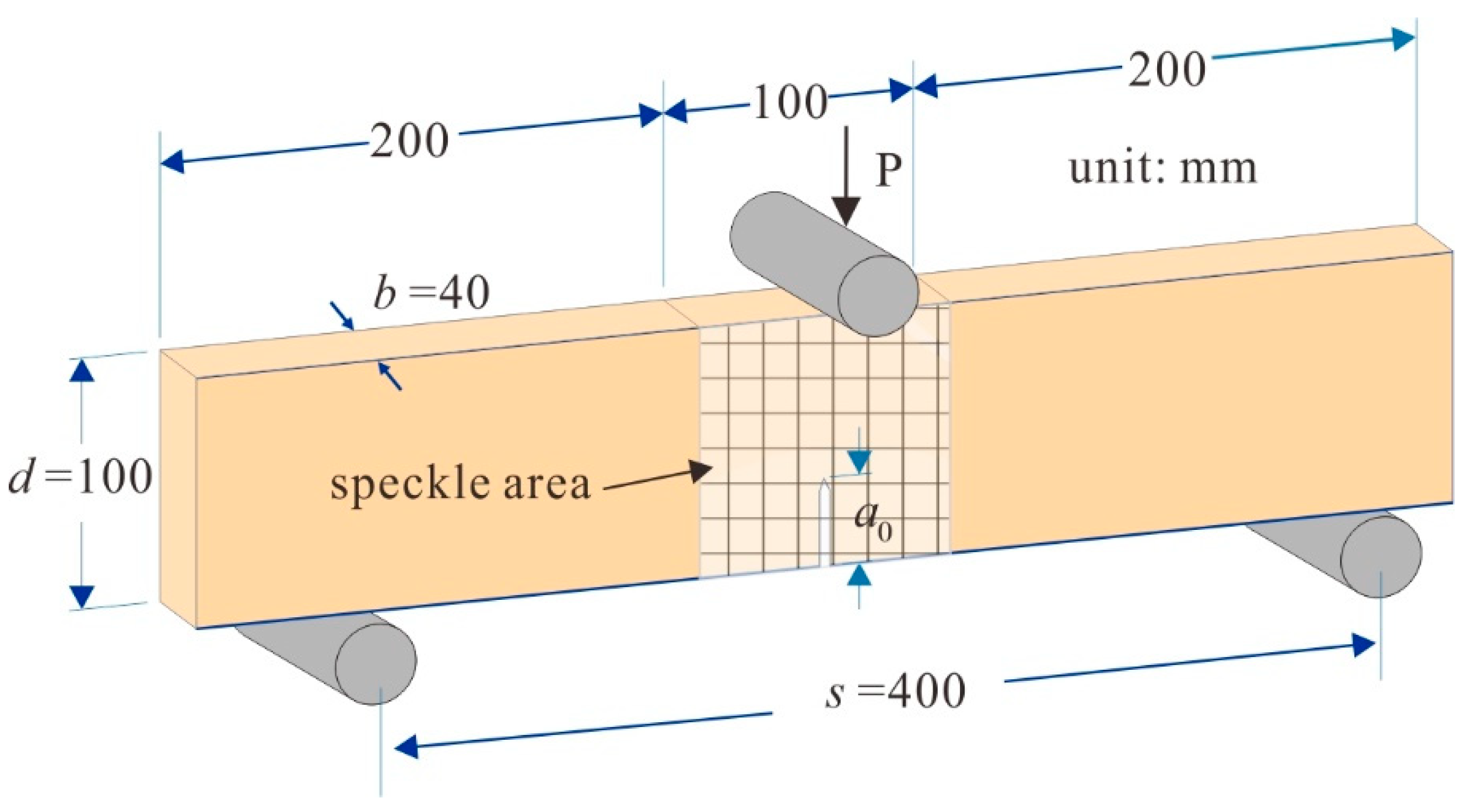
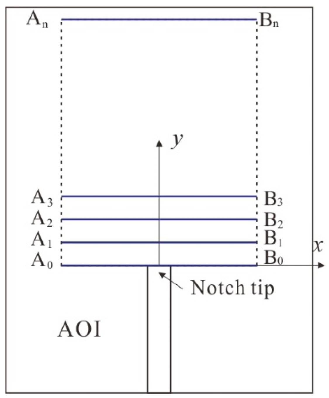
2.1. 3-p-b Fracture and DIC Test
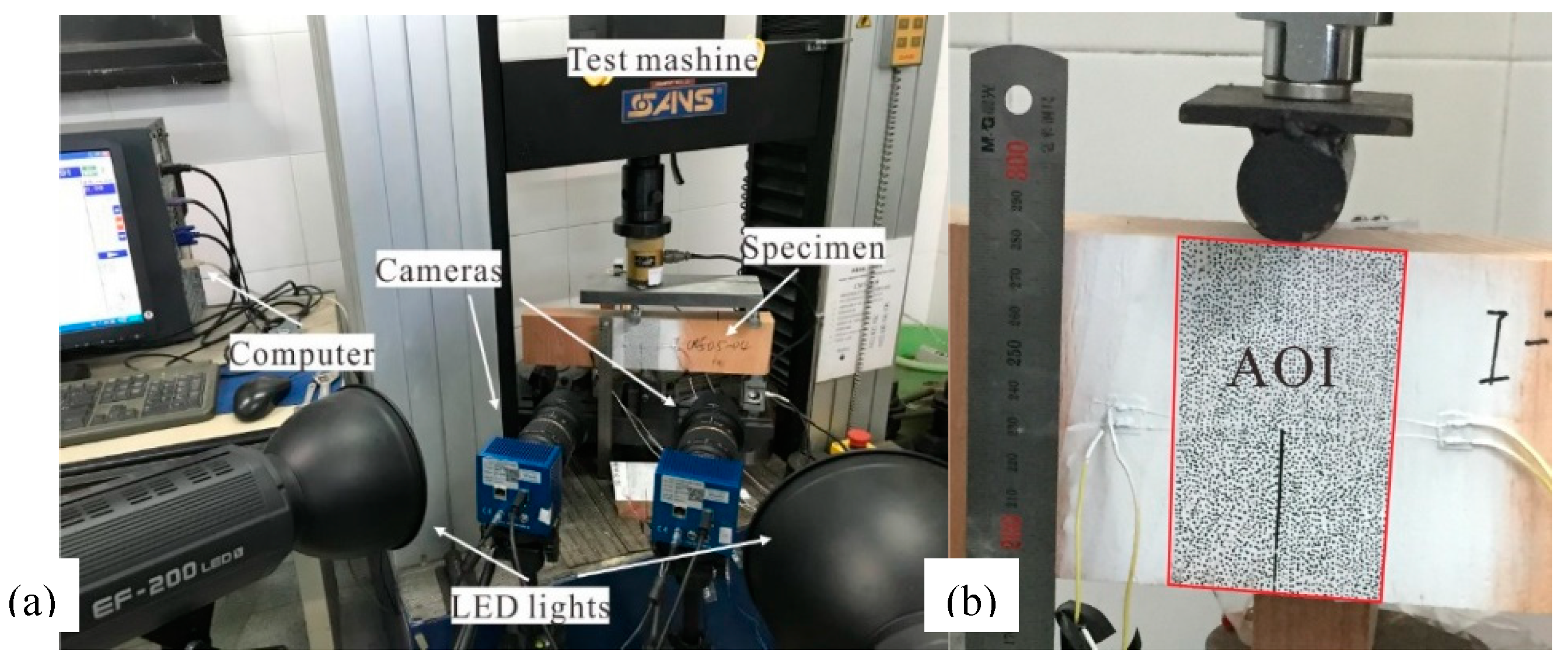
A 3-p-b flexural test on SEN beams was adopted to measure the mode-I fracture crack propagation in the L direction. The specimen geometry b × d × l (width × depth × length) = 40 mm × 100 mm × 500 mm with a span s of 400 mm is shown in Figure 1. The span-to-depth ratio was determined as s/d=4. Due to the size limit of sawn lumber, the specimen was symmetrically composed of three parts, for which the longitudinal direction was all oriented along the loading direction. The three parts were bonded together with epoxy adhesive. The initial notch was cut with a band saw of 2 mm thick, while the notch tip was prolonged with a razor blade with a thickness of 0.5 mm. Four groups of beams with different initial crack lengths a0 were prepared with three specimens for each group, as the initial crack length a0 was determined as 30, 40, 50 and 60 mm, in that the notch-to-depth ratio, a0/d, was 0.3, 0.4, 0.5 and 0.6. There were three specimens in each a0/d group, and each specimen was numbered as (a0/d)–n, e.g., specimen 0.3-1 is associated with the first specimen in the notch-to-depth ratio group, a0/d = 0.3.
As a result of the wood grain texture, the notch plane did not coincide with the TL or the RL system perfectly. As shown in Figure 2, there was an angle α between the notch plane and the L-T plane. Specimens with a value of α around 70° were prepared to exclude the effect of angle pattern on the fracture performance.
Heartwood of Douglas fir (Pseudotsuga menziesii) from Canada was used to make the specimens. The average width of a growth ring was about 6.7 mm, and the average oven dry specific density was 0.44 g/cm3. The moisture content was 13% during testing and the tensile strength in the L direction at this moisture was 85.0 MPa.

2.2. Test Set-Up

The 3-p-b test was carried out by a 10 kN electro-mechanical testing machine. The load P was applied along the grain direction, in the same plane of the pre-notch. Displacement control with a rate of 1 mm/min was adopted in order to reach the peak load Pmax in about 2 min to minimize possible viscoelastic effect. Two clip gauges with the measuring range of ± 2 mm were fixed on the side surface by knife edges to measure the crack mouth opening displacement (CMOD) and crack tip opening displacement (CTOD). Two cameras were placed one meter in front of the specimen to capture images continuously, and two high-power LED lights were placed next to the camera to provide sufficient light source, as shown in Figure 3a. The digital cameras had a resolution of 2310 × 1720 pixels and gave 256 levels of gray output. For this resolution, one pixel in the image represented approximately 69 μm on the specimen. The computation resolution of the DIC program was 0.01 pixels, so the measurement resolution was in the order of 0.69 μm, which was sufficient to determine the displacement measurement. The shooting frequencies of the two cameras were different: one was used to capture the whole fracture process with a shooting frequency of 20 pictures per second, and another was used to capture the propagation of the crack with a shooting frequency of 200 pictures per second. Data from the two cameras were synchronized over time, and then the Correlated Solutions software [22] was used to perform the DIC technique.
In the DIC technique, the essential importance in preparing the specimens is the uniqueness of the speckle pattern, especially the pattern within the subset [23,24,25,26,27]. A commercial software VIC-2D by Correlated Solution is adopted to do the correlation analysis [28]. We used a typical 21 × 21 subset with 70% overlap, and an analysis grid pixel spacing. For the strain calculation, VIC-2D uses a Gaussian filter where the data point at the centre is set a weight of one and data point at the edge of the circle are set as 0.1. The default filter size of 15 was used, which corresponds to 31pixel diameter circle.
To obtain a random speckle pattern, the surface of the specimen was sprayed evenly with ordinary white paint. After the paint dried, an unevenly distributed speckle pattern was created using a black pen. An area of 160 mm × 118 mm is captured as the field of view. Since the CCD array of the digital camera was fixed (14.5 pixel/mm), the average size of the speckle was about 5 mm (usually 3~5 speckle/pixel). Therefore, the diameter of the black pen was chosen as 0.5 mm. The speckle pattern and the area of interest (AOI) is presented in Figure 3b.

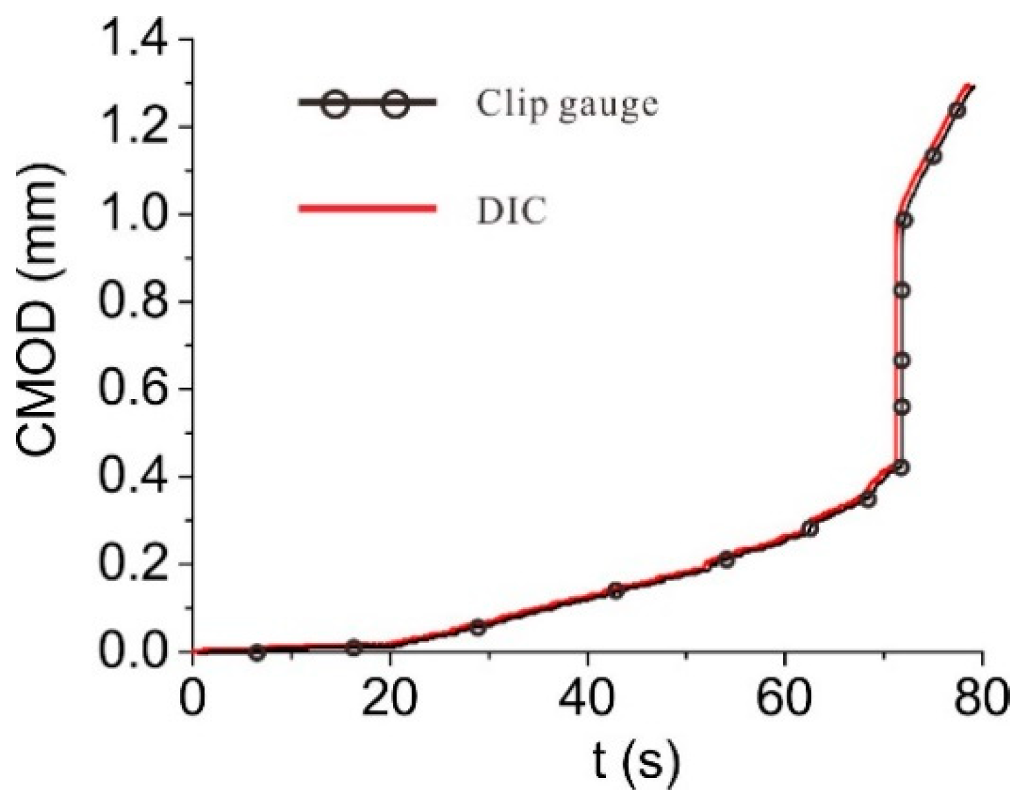
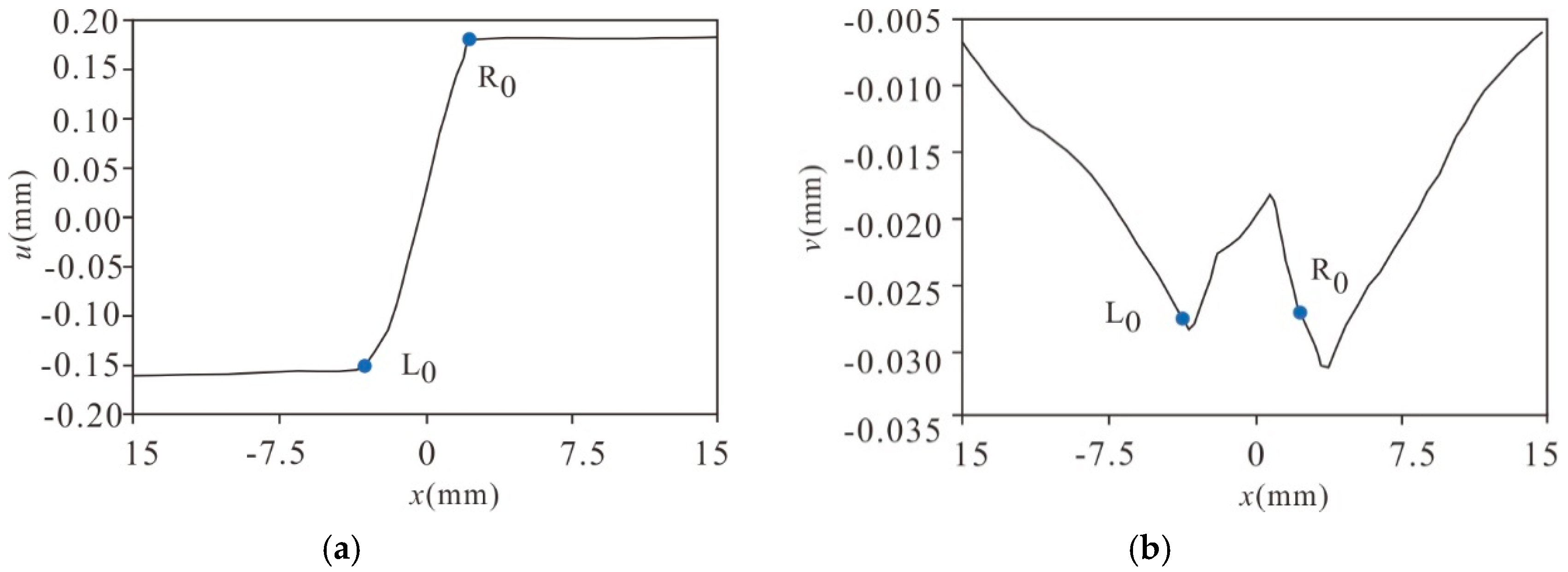
2.3. Verification of DIC Results

The DIC technique can be used to determine the CMOD by the relative displacement of two points on both sides of the crack tip [14,19]. To verify the DIC analysis, the measured CMOD values from the DIC technique and the clip gauge were compared with each other. Taking Specimen 0.3-3 as an example, the CMOD measured by these two methods agree well with each other, as illustrated in Figure 4, indicating that the DIC technique used here is suitable to accurately measure the displacement field of the crack propagation.

3. Results

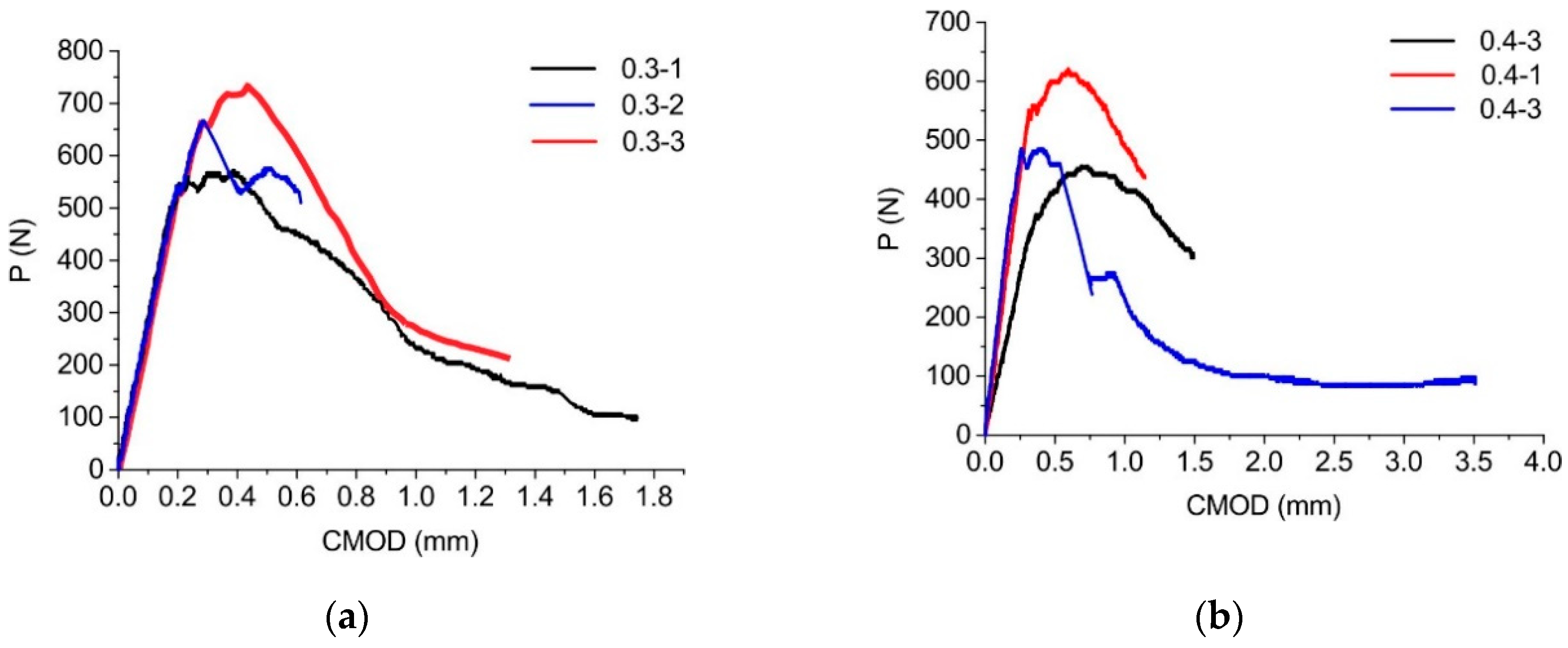
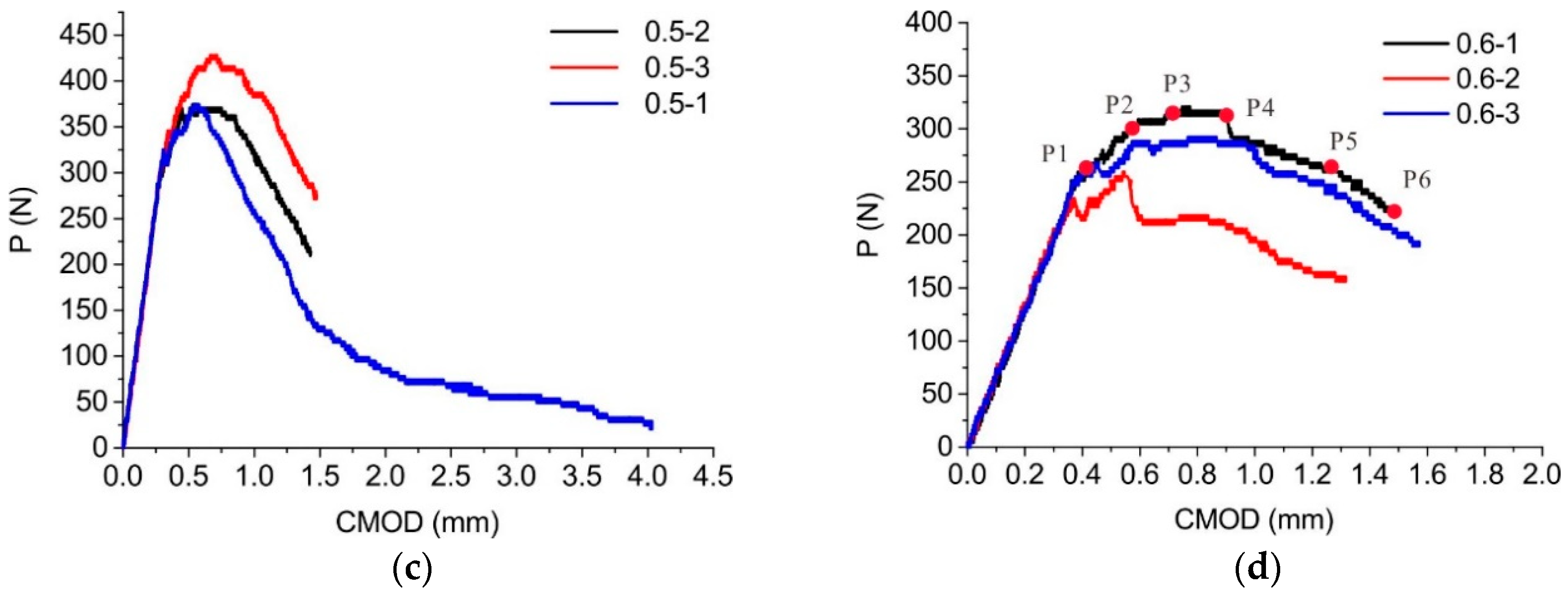
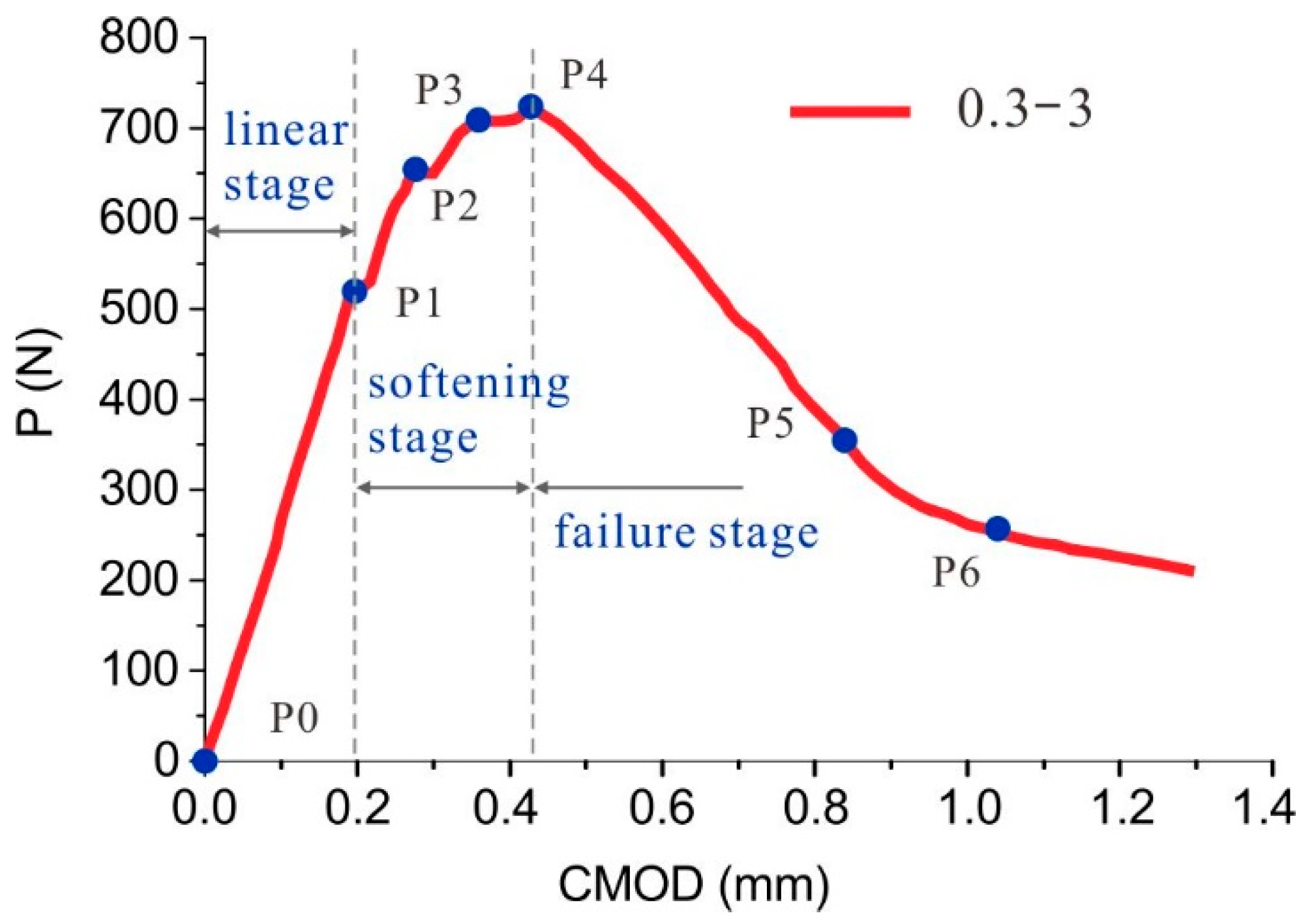
3.1. Quasi-Brittle Fracture Process of the Wood in the Longitudinal Direction

The P-CMOD curves (the relation between external load P and the crack mouth opening displacement) of all specimens are shown in Figure 5. All curves have a softening stage before the peak load Pmax, indicating that quasi-brittle fracture happens in the longitudinal direction of this kind of wood. On the other hand, the quasi-brittle fracture can be further explained by the crack propagation which is revealed by the strain fields measured by DIC in the X-axis direction of the specimen under various load points in different stages.
Take specimen 0.3-3 as an example. As is shown in Figure 6, the P-CMOD curve is divided into three stages: linear stage, softening stage, and failure stage, which are consistent with the crack development: crack formation, crack growth, and crack propagation, respectively. Six typical points, P1-P6, are selected from the 0.3-3 test curve. The speckle images of the failed specimen (area of 70 mm × 30 mm) at these loading points are shown in Figure 7. Although 267 images were obtained every second, it is difficult to see the difference of the crack between the first five images by human vision, before the crack propagates unsteadily. However, the corresponding horizontal strain fields obtained from DIC technique captured the entire progression of the crack tip (Figure 8).
No crack is formed in the first stage (0-P1). The CMOD increases due to the elastic deformation of the wood fibers and matrix. The load-deflection curve remains linear because the wood fibers have not been damaged. From Figure 8a, the strain field at this stage is symmetric with respect to the initial notch, that is, the vertical interface at x = 0 can be seen as a symmetric line where the initial notch is located. Most of the wood fibers are in elastic tension during this period. P1 can be considered at the starting point of the micro-cracks, and the specimen reaches the elastic limit at this point.
In the second stage (P1-P4), micro-cracks are formed around the initial notch tip due to stress concentrations. These micro-cracks around the preformed crack start to converge to macrocracks. Macroscopically, the strain field of the specimen is still symmetric, and the tip of the crack propagates steadily (Figure 8b–d). The load-deflection curve begins its non-linear softening relation from point P1. Because bunches of fibers peel and break due to the inside defects and externally increasing load, it is reasonable to have load oscillation in the second phase. What is more, at point P1, P2 and P3, the obvious “jump” phenomenon indicates that a big bunch of fibers break. Although the fibers are bent or peeled but adjacent fibers that are intact offer bending resistance and this leads to rise in the load until the Peak load (P4).
After the specimen reaches the Peak load (P4), it turns into the third stage. In this stage, the fibers in front of the notch tip are fully destroyed by micro-cracks. The crack propagates unsteadily and rapidly (Figure 8e,f). The specimen cannot bear the increasing load. Hence, the applied load has a sudden drop and the specimen fracture starts its failure stage. However, because of the fiber bridging effect, the specimen does not break into two parts immediately. As a result, CMOD increases rapidly with the decrease of load.

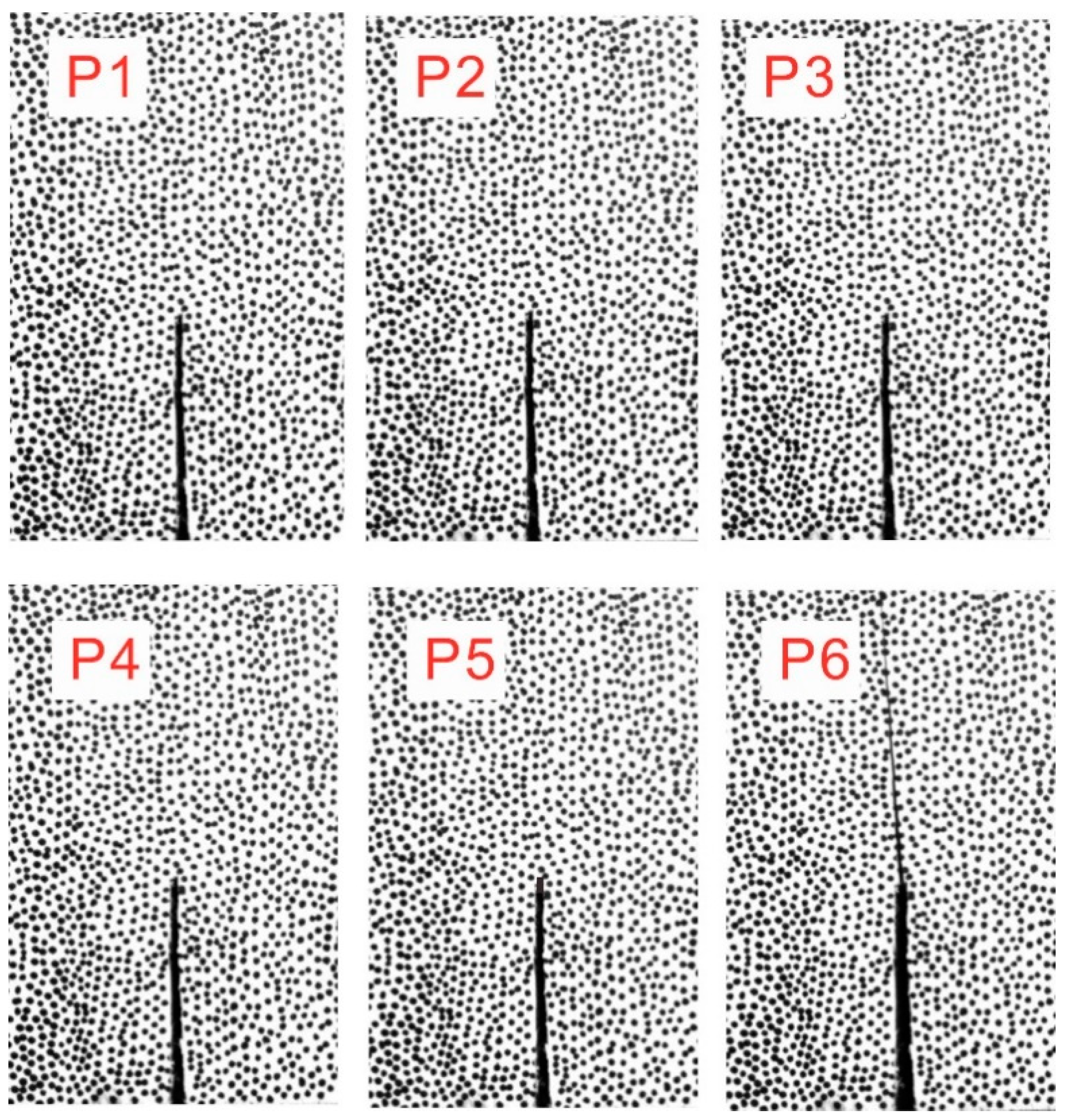
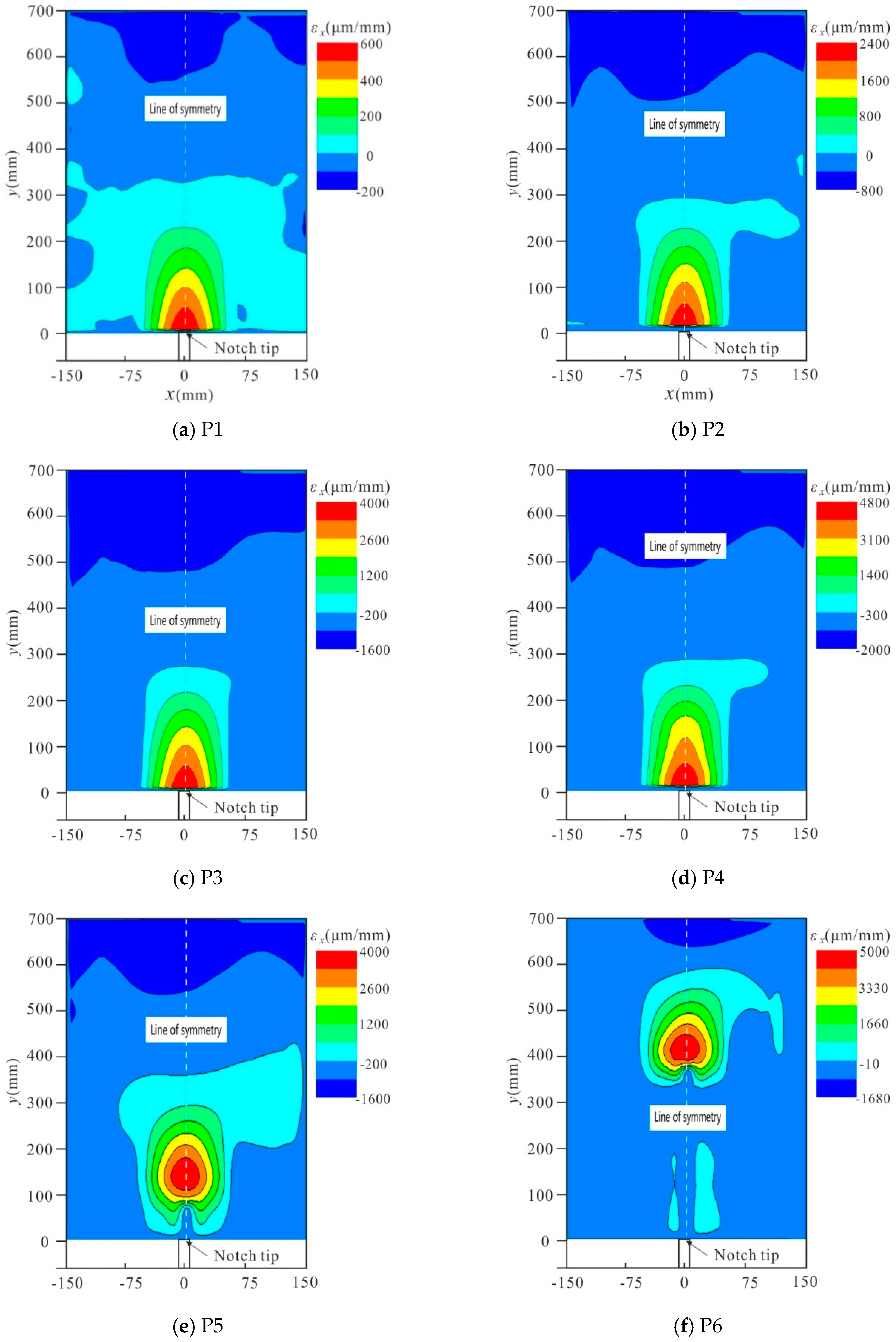
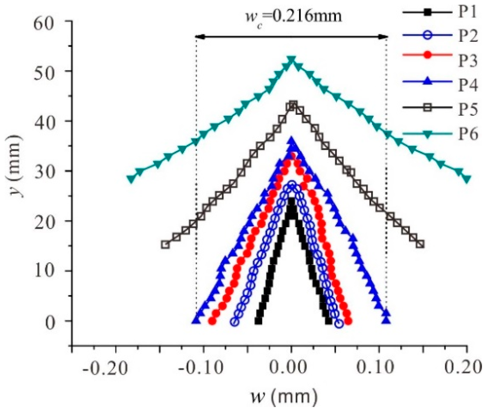
3.2. FPZ Evaluation by DIC Technique

Since the DIC technique can obtain the full field of specimen deformation, it can be used to determine the fracture process zone (FPZ) in accordance with the crack propagation. An analysis region with a width of 30 mm in front of the preformed crack was selected for analysis, as shown in the red box in Figure 9. First, a lateral line A0B0 is set in the x direction (perpendicular to the symmetry line) at the initial crack tip, and then a series of parallel lines, A1B1, A2B2,..., AnBn, are marked with an interval of 2 mm. The horizontal displacement u of each straight line along the x direction (indicating crack opening) and the vertical displacement v along the y direction (indicating crack sliding) are obtained by comparing the continuous speckle pictures. Then, the profile of the crack and the FPZ size at each loading point can be determined [14,18].
Take the specimen 0.3-3 as an example. Figure 10 represents the displacement of A0B0 along the x and y directions at loading point P5 (Figure 5a). Point L0 and R0 in Figure 10 represent the two boundary points at the jump of transverse displacement. The distance between L0 and R0 in Figure 10a is 0.335 mm, which represents the opening displacement of the crack on line A0B0. The sliding displacement at points L0 and R0 in Figure 10b are –0.0276 mm and 0.02684, respectively. So, the sliding displacement along the crack is much smaller than the transverse displacement, which agrees well with the properties of Mode I fracture [29]. In this way, the opening displacement and sliding displacement on A1B1, A2B2,..., and AnBn can be calculated, and the position of the crack tip can be obtained when the displacement of the inspected line reaches zero. With this method, the crack profile at the characteristic point of specimen 0.3-3 and specimen 0.6-1 are determined, as shown in Figure 11.

4. Discussion

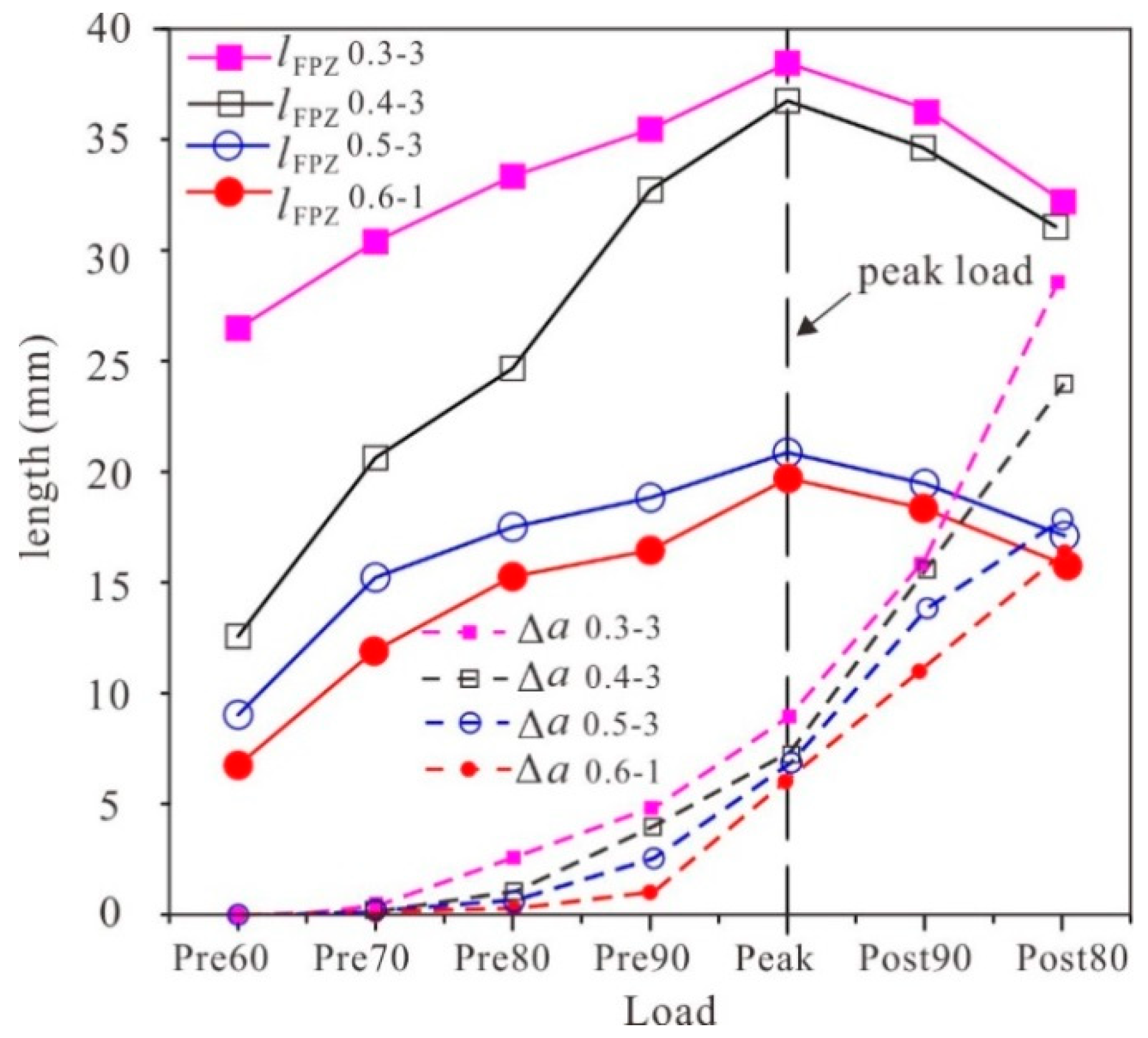
4.1. FPZ Development during the Fracture Process

During the fracture process, FPZ evolution is mainly divided into two stages: first, with increasing applied load, the FPZ size increases until the crack opening displacement (COD) reaches its maximum value, wc. Complete FPZ is formed at this time, and the length of the FPZ reaches the limit value. In the second stage, as the COD increases, the FPZ moves forward toward the loading point. According to the cohesive fracture model, it can be considered that the crack surface cannot transfer the tensile stress anymore, and a stress-free crack is formed when the COD is bigger than wc, Therefore, the length of the FPZ can be determined by the distance between the stress-free crack tip and the point where the normal stress reaches the ultimate tensile strength [9,30].
Apparently, the FPZ size depends on wc greatly. Therefore, it is rather important to determine the stress-free COD, wc. Hillerborg et al. [4] proposed the bilinear softening model that better describes the strain softening behavior of concrete, in which wc is 0.36 Gf/ft, while for the 3-p-b fracture test, the CTOD corresponding to the peak load was determined as wc [31]. This study also takes the measured CTOD value at the peak load as wc, then, the bottom point of the FPZ can be determined by comparing the horizontal displacement of lines A0B0, A1B1,..., and AnBn with the wc value. The top point of the FPZ is considered to be located at the fictitious crack tip. Thus, the FPZ length can be obtained. For example, for specimen 0.3-3 (Figure 11), wc is determined to be 0.22 mm (CTOD value at the peak load measured by the clip gauge). Before the peak load Pmax (P4 in Figure 6), the FPZ length is 23.97 mm (P1 in Figure 6) and 32.96 mm (P3 in Figure 6). When the applied load reaches Pmax, the cohesive zone is fully developed to form a complete FPZ with a maximum of 35.95 mm. After that, the CTOD increases dramatically, and accordingly, the FPZ moves forward fast. At the point P6, the FPZ length shrinks to 18.49 mm.
To compare the FPZ development of specimens with different initial crack length, the FPZ evolution of four specimens picked from each group are plotted in Figure 12. The x-axis indicates the proportion of the applied load with respect to the peak load, meanwhile, ‘pre’ and ‘post’ represent that the specimen is going through the fracture process before and after the peak load, respectively. It is seen that the FPZ length exhibits the same trend as the applied load. As the load increases, the FPZ length increases continuously, and as the load decreases after the peak load, the FPZ length decreases rapidly. Additionally, the notch-to-depth ratio, a0/d, has a great impact on the FPZ length, in that smaller a0/d has a longer FPZ length. Since a relatively longer FPZ length will provide a better cohesive effect and a higher cracking resistance, the specimen with smaller a0/d has a better resistance to crack propagation.

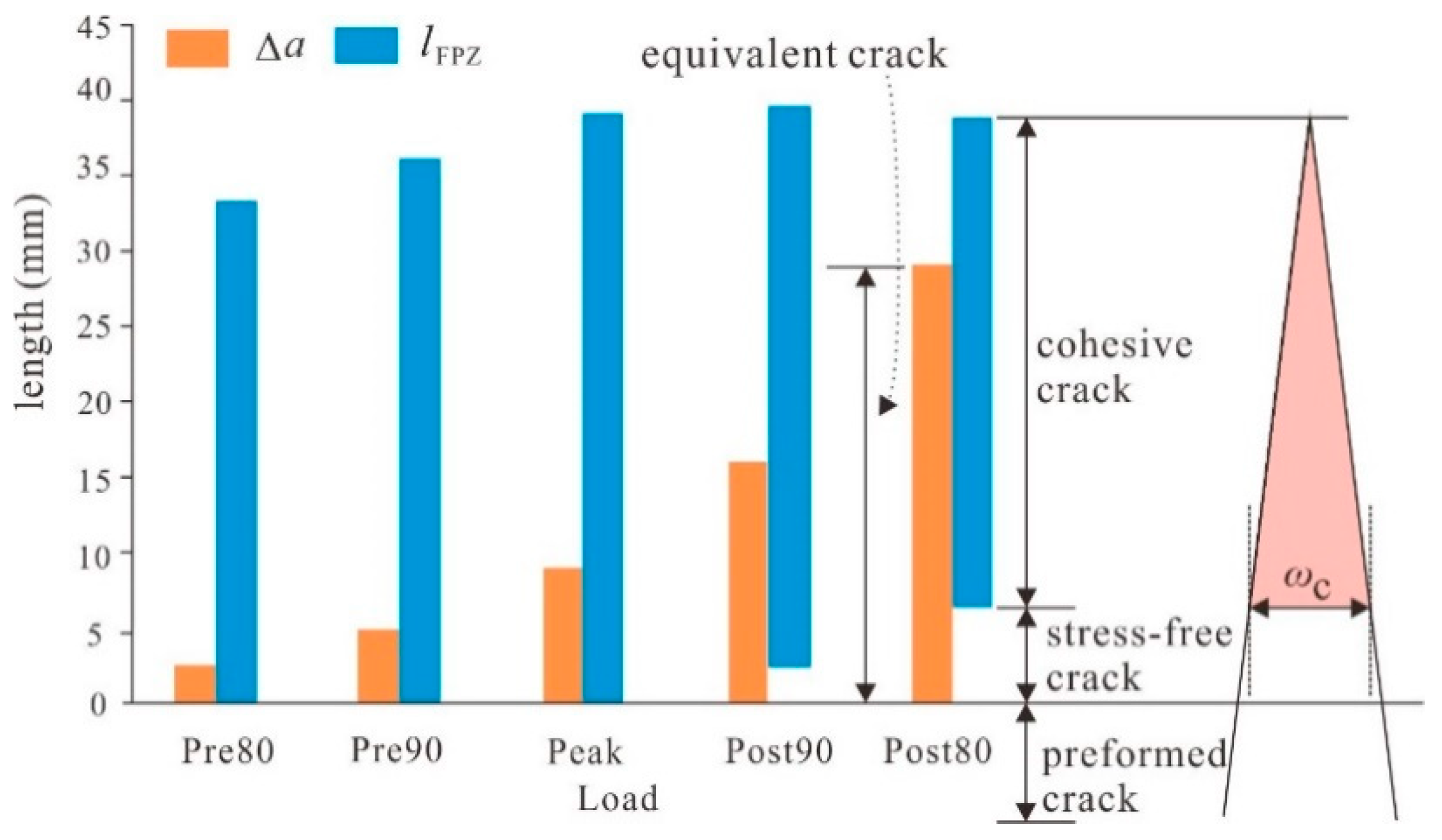
4.2. Comparison between the Equivalent Elastic Crack and FPZ

For brittle material, the fracture properties, such as fracture toughness KI, are well defined according to linear elastic fracture mechanics (LEFM). However, due to the crack bridging effect during the crack propagation, LEFM cannot be directly applied to quasi-brittle fracture in wood [3]. The equivalent elastic crack of length aeq is one of the fundamental parameters used to modify the LEFM. If aeq of the quasi-brittle material can be determined accurately, the equations in LEFM can still be used to evaluate its quasi-brittle fracture. In this study, the linear superposition hypothesis for quasi-brittle fracture in double-K fracture criterion [32,33] is used to calculate aeq. According to LEFM, for mode I fracture, P has the following relationship with CMOD, as shown in Equation (1) [34]. Based on this equation, three points in the linear stage of the P-CMOD curve are selected to calculate three longitudinal elastic moduli, which are averaged to determine the longitudinal elastic modulus E of the specimens. Then, according to Equation (1), the corresponding critical crack length ac is calculated using the external peak load P, CMOD and elastic modulus E.
CMOD = 24 P a b d E V 1 ( a / d ) V 1 ( a / d ) = 0.76 2.28 a / d + 3.87 ( a / d ) 2 2.04 ( a / d ) 3 + 0.66 ( 1 a / d ) 2
The crack increment, Δa = aeqa0, is plotted in Figure 12. It is shown that the specimen with smaller a0/d has a larger Δa, and thus dissipates more fracture energy, which agrees well with the FPZ evolution. Taking the specimen 0.3-3 as an example, the developments of FPZ and aeq are compared in Figure 13. It can be seen that FPZ propagates at the beginning of loading, while the aeq begins around ‘Pre60~Pre70’. Moreover, FPZ decreases after the peak load while aeq develops longer and faster in this stage.

5. Conclusions

Using the DIC technique, the FPZ evolution and crack propagation of Douglas fir during its quasi-brittle fracture process along the longitudinal direction were studied. The DIC technique is verified by comparing the CMOD values obtained from it and measured by clip gauges. According to images of the failed specimen, the P-CMOD curve and strain field in front of the crack tip, the quasi-brittle fracture process is clearly divided into a linear stage, softening stage and failure stage.
The crack propagation is obtained using the DIC technique by measuring the computational grids in front of the crack tip. Then the FPZ is determined based on the crack propagation and the critical CTOD value at the peak load point. The equivalent elastic crack aeq is calculated using the linear superposition hypothesis. Combing FPZ and aeq, properties about wood fracture are given. The FPZ propagates at the beginning of loading, while the aeq starts around ‘Pre60~Pre70’. FPZ decreases after the peak load, but aeq develops longer and faster after the peak load. Additionally, specimens with smaller notch-to-depth ratios have better cohesive effect and a higher cracking resistance.
It must be noted that the CTOD at the peak load is set as wc in this work, which may need more consideration in the future. Also, the R-cures of wood fracture can be established to determine the critical crack length of this material.

Author Contributions

Data curation, W.Z.; Investigation, H.Z.; Writing—original draft, Y.Y.; Writing—review & editing, W.L. and X.W.

Funding

This research was funded by the National Key Research and Design Program of China (2017YFC0806100), Natural Science Foundation of Guangdong, China (2018A030307030), the China Scholarship Council (201808440059), Guangdong Science and Technology Program, China (180917114960497) and Shantou Science and Technology Program, China (2016-37).

Conflicts of Interest

The authors declare no conflict of interest. The funders had no role in the design of the study; in the collection, analyses, or interpretation of data; in the writing of the manuscript, and in the decision to publish the results.

References

  1. Smith, I.; Landies, E.; Gong, M. Fracture and Fatigue in Wood; John Wiley & Sons, Ltd.: New Jersey, NJ, USA, 2003. [Google Scholar]
  2. Stanzl-Tschegg, S.E.; Tan, D.M.; Tschegg, E.K. New splitting method for wood fracture characterization. Wood Sci. Technol. 1995, 29, 31–50. [Google Scholar] [CrossRef]
  3. De Moura, M.F.S.F.; Dourado, N. Wood Fracture Characterization; CRC Press: Boca Raton, FL, USA, 2018. [Google Scholar]
  4. Hillerborg, A.; Modéer, M.; Petersson, P.E. Analysis of crack formation and crackgrowth in concrete by means of fracture mechanics and finite elements. Cem. Concr. Res. 1976, 6, 773–781. [Google Scholar] [CrossRef]
  5. Morel, S.; Lespine, C.; Coureau, J.-L.; Planas, J.; Dourado, N. Bilinear softening parameters and equivalent LEFM R-curve in quasibrittle failure. Int. J. Solids Struct. 2010, 47, 837–850. [Google Scholar] [CrossRef] [Green Version]
  6. Yoshihara, H.; Satoh, A. Shear and crack tip deformation correction for the double cantilever beam and three-point-end-notched flexure specimens for mode I and mode II fracture toughness measurement of wood. Eng. Fract. Mech. 2009, 76, 335–346. [Google Scholar] [CrossRef]
  7. De Moura, M.F.S.F.; Morais, J.J.L.; Dourado, N. A new data reduction scheme for mode I wood fracture characterization using the double cantilever beam test. Eng. Fract. Mech. 2008, 75, 3852–3865. [Google Scholar] [CrossRef]
  8. Hu, X.; Duan, K. Size effect: Influence of proximity of fracture process zone to specimen boundary. Eng. Fract. Mech. 2007, 74, 1093. [Google Scholar] [CrossRef]
  9. Dai, Y.; Gruber, D.; Harmuth, H. Observation and quantification of the fracture process zone for two magnesia refractories with different brittleness. J. Eur. Ceram. Soc. 2017, 37, 2521–2529. [Google Scholar] [CrossRef]
  10. Watanabe, K.; Shida, S.; Ohta, M. Evaluation of end-check propagation based on mode I fracture toughness of sugi (Crytomeria japonica). J. Wood Sci. 2011, 57, 371–376. [Google Scholar] [CrossRef]
  11. Reiterer, A.; Sinn, G.; Stanzl-Tschegg, S.E. Fracture characteristics of different wood species under mode I loading perpendicular to the grain. Mat. Sci. Eng. A Struct. 2002, 332, 29–36. [Google Scholar] [CrossRef]
  12. Alam, S.Y.; Saliba, J.; Loukili, A. Fracture examination in concrete through combined digital image correlation and acoustic emission techniques. Constr. Build. Mater. 2014, 69, 232–242. [Google Scholar] [CrossRef] [Green Version]
  13. Cai, M.F.; Liu, D.M. Study of failure mechanisms of rock under compressive–shear loading using real-time laser holography. Int. J. Rock Mech. Min. Sci. 2009, 46, 59–68. [Google Scholar] [CrossRef]
  14. Lin, Q.; Fakhimi, A.; Haggerty, M.; Labuz, J.F. Initiation of tensile and mixed-mode fracture in sandstone. Int. J. Rock Mech. Min. Sci. 2009, 46, 489–497. [Google Scholar] [CrossRef]
  15. Sciammarella, C.; Sciammarella, A.; Federico, M. Experimental Mechanics of Solids; John Wiley & Sons, Ltd.: Chichester, UK, 2012; pp. 607–629. [Google Scholar]
  16. Gencturk, B.; Hossain, K.; Kapadia, A.; Labib, E.; Mo, Y.L. Use of digital image correlation technique in full-scale testing of prestressed concrete structures. Measurement 2014, 47, 505–515. [Google Scholar] [CrossRef]
  17. Yates, J.R.; Zanganeh, M.; Tai, Y.H. Quantifying crack tip displacement fields with DIC. Eng. Fract. Mech. 2010, 77, 2063–2076. [Google Scholar] [CrossRef]
  18. Lin, Q.; Labuz, J.F. Fracture of sandstone characterized by digital image correlation. Int. J. Rock Mech. Min. Sci. 2013, 60, 235–245. [Google Scholar] [CrossRef]
  19. Dong, W.; Wu, Z.M.; Zhou, X.M.; Dong, L.H.; Kastiukas, G. An experimental study on crack propagation at rock-concrete interface using digital image correlation technique. Eng. Fract. Mech. 2017, 171, 50–63. [Google Scholar] [CrossRef]
  20. Morel, S.; Mourot, G.; Schmittbuhl, J. Influence of the specimen geometry on R-curve behavior and roughening of fracture surfaces. Int. J. Fract. 2003, 121, 23–42. [Google Scholar] [CrossRef]
  21. Coureau, J.L.; Morel, S.; Dourado, N. Cohesive zone model and quasibrittle failure of wood: A new light on the adapted specimen geometries for fracture tests. Eng. Fract. Mech. 2013, 109, 328–340. [Google Scholar] [CrossRef]
  22. Correlated Solutions. VIC-2D Reference Manual; Correlated Solutions, Inc.: Columbia, SC, USA, 2014. [Google Scholar]
  23. Lamberti, L.; Lin, M.T.; Furlong, C.; Sciammarella, C.; Phillip, L.R.; Michael, A.S. Advancement of Optical Methods & Digital Image Correlation in Experimental Mechanics; Springer: New York, NY, USA, 2018; Volume 3. [Google Scholar]
  24. Patel, J.; Peralta, P. Mechanisms for Kink Band Evolution in Polymer Matrix Composites: A Digital Image Correlation and Finite Element Study. In Mechanics of Solids, Structures and Fluids; NDE, Diagnosis, and Prognosis, Proceedings of the ASME International Mechanical Engineering Congress and Exposition, Phoenix, AZ, USA, 11–17 November 2016; ASME: New York, NY, USA, 2016; Volume 9. [Google Scholar] [CrossRef]
  25. Nizolek, T.J.; Begley, M.R.; McCabe, R.J.; Avallone, J.T.; Mara, N.A.; Beyerlein, I.J.; Pollock, T.M. Strain fields induced by kink band propagation in Cu-Nb nanolaminate composites. Acta Mater. 2017, 133, 303–315. [Google Scholar] [CrossRef]
  26. Ye, X.W.; Dong, C.Z.; Liu, T. Image-based structural dynamic displacement measurement using different multi-object tracking algorithms. Smart Struct. Syst. 2016, 17, 935–956. [Google Scholar] [CrossRef]
  27. Ye, X.W.; Yi, T.H.; Dong, C.Z.; Liu, T. Vision-based structural displacement measurement: System performance evaluation and influence factor analysis. Measurement 2016, 88, 372–384. [Google Scholar] [CrossRef] [Green Version]
  28. Correlated Solutions. Vic-2D Manual; Correlated Solutions, Inc.: Columbia, SC, USA, 2010; Available online: www.correlatedsolutions.com (accessed on May 31 2010).
  29. John, T.W. Relating Cohesive Zone Models to Linear Elastic Fracture Mechanics; NASA Langley Research Center: Hampton, VA, USA, 2010.
  30. Barris, C.; Torres, L.; Vilanova, I.; Miàs, C.; Llorens, M. Experimental study on crack width and crack spacing for Glass-FRP reinforced concrete beams. Eng. Struct. 2017, 2013, 231–242. [Google Scholar] [CrossRef]
  31. Petersson, P.E. Crack Growth and Development of Fracture Zones in Plain Concrete and Similar Materials. Doctoral Dissertation; Lund Institute of Technology: Lund, Sweden, 1981. [Google Scholar]
  32. Xu, S.L.; Reinhardt, H.W. Determination of double-K criterion for crack propagation in quasi-brittle fracture, Part I: Experimental investigation of crack propagation. Int. J. Fract. 1999, 98, 111–149. [Google Scholar] [CrossRef]
  33. Xu, S.L.; Reinhardt, H.W. Determination of double-K criterion for crack propagation in quasi-brittle fracture, Part II: Analytical evaluating and practical measuring methods for three-point bending notched beams. Int. J. Fract. 1999, 98, 151–177. [Google Scholar] [CrossRef]
  34. Tada, H.; Paris, P.C.; Irwin, G.R. The Stress Analysis of Cracks Handbook; ASME Press: New York, NY, USA, 2000. [Google Scholar]
Figure 1. Specimen geometry and loading condition.
Remotesensing 11 01562 g001
Figure 2. The angle α between the LT plane (the red dotted areas) and the crack plane (the black dotted areas).
Remotesensing 11 01562 g002
Figure 3. (a) Two cameras used to capture images continuously; (b) the area of interest (AOI) and speckle pattern on specimen surface.
Remotesensing 11 01562 g003
Figure 4. Comparison of the crack mouth opening displacements (CMOD) measured by the digital image correlation (DIC) technique and the clip gauge.
Remotesensing 11 01562 g004
Figure 5. The experimental curves P-CMOD of the four group specimens. (a) a0/d = 0.3, (b) a0/d = 0.4, (c) a0/d = 0.5, (d) a0/d = 0.6.
Remotesensing 11 01562 g005aRemotesensing 11 01562 g005b
Figure 6. Three stages for typical P-CMOD curve of specimen 0.3-3.
Remotesensing 11 01562 g006
Figure 7. Speckle image of the specimen 03-3 at different loading points.
Remotesensing 11 01562 g007
Figure 8. Horizontal strain contours of specimen 0.3-3 at different load points: (a) P1; (b) P2; (c) P3; (d) P4; (e) P5; (f) P6.
Remotesensing 11 01562 g008
Figure 9. Computational grids for Specimen 0.3-3 in the AOI.
Remotesensing 11 01562 g009
Figure 10. Displacement on line A0B0 of specimen 0.3-3 at loading P5: (a) opening displacement, (b) sliding displacement.
Remotesensing 11 01562 g010
Figure 11. Crack propagation of specimen 0.3-3.
Remotesensing 11 01562 g011
Figure 12. Evolution of the fracture process zone (FPZ) and the equivalent elastic crack.
Remotesensing 11 01562 g012
Figure 13. The propagation of FPZ and Δa for specimen 0.3-3.
Remotesensing 11 01562 g013

