A Full-Coverage Daily Average PM_2.5 Retrieval Method with Two-Stage IVW Fused MODIS C6 AOD and Two-Stage GAM Model

Abstract

Current PM_2.5 retrieval maps have many missing values, which seriously hinders their performance in real applications. This paper presents a framework to map full-coverage daily average PM_2.5 concentrations from MODIS C6 aerosol optical depth (AOD) products and fill missing pixels in both the AOD and PM_2.5 maps. First, a two-stage inversed variance weights (IVW) algorithm was adopted to fuse the MODIS C6 Terra and Aqua AOD products, which fills missing data in MODIS standard AOD data and obtains a high coverage daily average. After that, using the fused MODIS daily average AOD and ground-level PM_2.5 in all grid cells, a two-stage generalized additive model (GAM) was implemented to obtain the full-coverage PM_2.5 concentrations. Experiments on the Yangtze River Delta (YRD) in 2013–2016 were carefully designed to validate the performance of our proposed framework. The results show that the two-stage IVW could not only improve the spatial coverage of MODIS AOD against the original standard product by 230%, but could also keep its data accuracy. When compared with the ground-level measurements, the two-stage GAM can obtain accurate PM_2.5 concentration estimates (R² = 0.78, RMSE = 19.177 μg/m³, and RPE = 28.9%). Moreover, our method performs better than the inverse distance weighted method and kriging methods in mapping full-coverage daily PM_2.5 concentrations. Therefore, the proposed framework provides a good methodology for retrieving full-coverage daily average PM_2.5 concentrations from MODIS standard AOD products.

1. Introduction

The rapid growth of the extensive economy in China during last three decades brings about many ecological and environmental problems, especially the air pollution problem [1,2,3]. Most of the developed regions in China have been experiencing severe particulate matter pollution problems, e.g., the North China Plain (NCP) [4,5], the Yangtze River Delta region (YRD) [6,7] and the Pearl River Delta region (PRD) [8,9]. Particulate matter with an aerodynamic diameter less than 2.5 μm (PM_2.5) is one of most harmful particulate matters [10,11]. A high PM_2.5 concentration in the air results in a greater probability of lung cancer and mortality from it [12,13]. Therefore, monitoring PM_2.5 concentrations is of great importance for making effective air pollution control measures to reduce its harms.

Satellite-based remote sensing has been becoming a widely used technique to monitor the PM_2.5 concentrations [14,15,16]. It can provide a large spatial coverage of PM_2.5 concentrations over long periods, and this distinct advantage is unavailable for ground monitoring stations. Many satellite sensors like MODIS, MISR, SeaWiFS, AVHRR and OMI collect the aerosol information in the atmosphere including aerosol scattering and absorption [17]. Particularly, the higher spatial and temporal resolutions, larger imaging width and shorter revisiting cycle of MODIS make it the most widely used data source [18,19,20], and therefore we focus on MODIS in this study. The most recent version of MODIS C6 aerosol optical death (AOD) products include the dark blue (DB) and dark target (DT) versions retrieved from both Terra (10:30 a.m. in local time) and Aqua (1:30 p.m. in local time) satellites [21,22,23]. The AOD is a measure of columnar light extinction by aerosol scattering and absorption. The MODIS satellite estimates large-scale coverage of PM_2.5 concentrations via the retrieval model between ground PM_2.5 and the satellite-based AOD [15,24].

Many retrieval modes have been proposed to estimate PM_2.5 concentrations from MODIS AOD, and they can be roughly classified into three types [25]: (1) the scaling factor models [26,27], the semi-empirical physical analysis models [15,28], and the empirical statistical models [29]. The earliest are the scaling factor models, which determine the sale factor between MODIS AOD and ground PM_2.5 concentrations to estimate spatial distributions of PM_2.5. These models can be applied in atmospheric regions without ground PM_2.5 monitoring sites, but they always bring about low accuracy and are particularly unsuitable for estimating short-term average PM_2.5 concentrations (e.g., daily average, monthly average and even seasonal average) [29]. After that, the semi-empirical physical models were presented to improve the accuracy of PM_2.5 and they have been shown to behave better than the scale factor models. They investigate physical relationships between MODIS AOD and ground PM_2.5 and adopt physical parameters (e.g., humidity, particle size and vertical profile characteristics of AOD) to formulate retrieval functions [30,31]. Unfortunately, the involved physical parameters could not fully explain the complicated relationships between MODIS AOD and ground PM_2.5. Meanwhile, the difficulty in obtaining some key parameters severely limits their application performance [32]. In contrast, empirical statistical models also involve physical parameters and could generate more accurate distribution retrievals of PM_2.5 concentrations than the above two kinds of models [33]. In particular, the advanced statistical models could well delineate spatial–temporal variations in the relations between MODIS AOD and ground PM_2.5 measurements. Typical examples are the geographical weighted regression model (GWR) [34,35], the linear mixed effects (LME) [36] and the geographically and temporarily weighted regression model (GTWR) [37].

Numerous achievements have been made based on advanced statistical models to monitor large-scale spatial distribution of PM_2.5 concentrations, and much supporting data can be found in the literature, e.g., Liu [17,38], Ma [16,36], Van [39,40], Kloog [41,42]. However, obtaining accurate PM_2.5 concentrations with full coverage is still challenging [16,43,44], because of data incompleteness of MODIS AOD and drawbacks of statistical models. On the one hand, the cloud contamination and the characteristics of AOD inversion algorithms result in missing data in the MODIS AOD product [45]. This reduces the number of AOD samples available for PM_2.5 retrieval modeling and leads to bias and incompleteness of estimated PM_2.5 concentrations in spatial distributions. On the other hand, the PM_2.5 estimates from empirical statistical models depend on the correlations between ground PM_2.5 and MODIS AOD. These models could not offer spatially distributed PM_2.5 estimates without ground PM_2.5 observations. Fortunately, some researchers have tried to fill missing MODIS AOD data and estimate full-coverage daily PM_2.5 concentrations [46]. Bi et al. [47] examined the impacts of snow and cloud cover on AOD and PM_2.5 and made full coverage PM_2.5 predictions by considering the relationship of snow–AOD. Daily gap filling models with snow/cloud fractions and meteorological covariates were developed to estimate the missing AOD, using the random forest algorithm. Hu et al. [48] adopted the fixed rank smoothing to fill the data gaps in 3 km AOD data, and proposed a spatiotemporal regression kriging (STRK) model to obtain accurate daily PM_2.5 estimations with full-coverage. Zhao [49] and Vu [50] used the random forest model to estimate the corresponding full-coverage AOD data. Xue et al. [51] developed a machine learning model with high dimensional expansion of numerous predictors and incorporated a generalized additive model into the model to obtain a full-coverage PM_2.5 estimation. However, many of the above works have some specific prerequisites, which might limit their performances in realistic applications.

The YRD region is one of the fast-growing economic areas in China and has been experiencing severe PM_2.5 pollution. Ma presented a nested linear mixed effects (LME) model to estimate the high resolution PM_2.5 concentrations in the YRD of China from 3 km MODIS AOD [36]. The LME model has been proven to successfully describe the nested month-, week-, and day-specific random effects of PM_2.5–AOD relationships. Unfortunately, the LME model does not handle the problem of missing AOD values and cannot obtain full-coverage of PM_2.5 concentrations in the YRD. Later, Xiao proposed a multiple imputation (IM) method to fill missing AOD values and predicted the full-coverage PM_2.5 concentrations in the YRD from 2013 to 2014 [52]. The IM combines the multiangle implementation of atmospheric correlation (MAIAC) AOD with community multiscale air quality (CMAQ) simulations to fill missing AOD values, and it implements a two-stage statistical model to estimate the daily ground PM_2.5 concentrations. The specific MAIAC AOD product and the complicated CMAQ model limit the applicability of the IM method. In this paper, we would like to propose an innovative framework to retrieve full-coverage daily average PM_2.5 concentrations from MODIS C6 AOD data in the YRD for 2013–2016. Our idea is to fill partial missing MODIS AOD values and then predict the full-coverage PM_2.5 concentrations. Both the MODIS C6 AOD data and the idea of the proposed framework are different from above studies. More specifically, our framework is formulated on the statistical relationships between PM_2.5 concentrations and MODIS AOD, and it is much easier to implement than others. The spatial–temporal correlations between MODIS DB and DT AOD data from Terra and Aqua satellites provide a high probability of accurately estimating the missing AOD values in the standard product. Therefore, a two-stage version of the inverse variance weights (IVW) [53] algorithm is presented to iteratively fuse the MODIS DB and DT AOD from the Terra and Aqua satellites. By considering the divergent weights of different MODIS AOD data in the fusion procedure, the first-stage IVW fuses the DB and DT AOD data from the Terra and Aqua satellites, respectively. The second IVW performs a further fusion of the filled Terra and Aqua data to continue improving the spatial coverage of MODIS AOD data. After that, using the fused daily average MODIS AOD data, a two-stage generalized additive model (GAM) is implemented to obtain the full-coverage PM_2.5 concentrations. The GAM model considers complicated nonlinear relations between ground-level PM_2.5 and AOD and other explanatory variables (e.g., meteorological and geographic factors), and can automatically select smooth functions to fit explanatory variables and formulate the proper retrieval model [54]. The first-stage GAM investigates the temporal variations of ground PM_2.5 and predicts the PM_2.5 concentrations from the fused MODIS AOD, and the second-stage GAM adopts more spatial smooth factors to retrieve PM_2.5 concentrations for the pixels without the corresponding MODIS AOD.

The rest of our paper is arranged as follows. Section 2 describes the study area and the data used in the study. Section 3 presents the main methodology. Section 4 presents the experiments on the YRD region over four years, i.e., 2013–2016. Section 5 discusses the experimental results and Section 6 draws the conclusions.

2. Study Area and Data

2.1. Ground-Level PM_2.5 Observations

Our study area is located in the YRD region of China, including Shanghai city, Zhejiang, Jiangsu, and Anhui provinces. The YRD region covers an area of 350,600 km², taking 3.63% of the total area of China [1,2]. It belongs to a typical monsoon climate, having warm and humid weather in summer and cold and dry weather in winter. Ground-level hourly PM_2.5 concentration observations from 2013–2016 were downloaded from the China air quality real-time release system of the Chinese Ministry of Environmental Protection (available at http://106.37.208.233:20035). The PM_2.5 concentrations were measured by tapered element oscillating microbalances (TEOM) or the beta attenuation method (BAM or β-gauge). The data has an uncertainty less than 0.75%, with its accuracy reaching up to ±1.5 μg/m³ for the hourly average, and hence it is accurate enough as ground truth for PM_2.5 concentration measurements. Figure 1 illustrates the 245 ground monitoring stations of PM_2.5 in the YRD in 2016.

2.2. MODIS C6 and AERONET AOD Data

The latest MODIS AOD product version Collection 6 is constructed from the MODIS imagery using both the enhanced DB and DT algorithm, and the AOD product is adaptable for both dark and bright surfaces. In this study we utilized the MODIS C6 DB/DT AOD products from Level 2 and the Atmosphere Archive & Distribution System of NASA, and the DB/DT AOD products have two versions of MOD04 (Terra) and MYD04 (Aqua) [55] (available at https://ladweb.nascom. nasa.gov/search/). Considering the data quality of the MODIS C6 AOD product, the data with flags from 1 to 3 were used, and the data with flag = 0 were discarded.

The ground AERONET AOD data was used to validate the accuracy of retrieved AOD from MODIS satellite imagery [56]. The AERONET collaboration network provides globally distributed observation of AOD (available at https://AERONET.gsfc.nasa.gov/), and the AERONET data has three data quality levels: Level 1.0 (unscreened), Level 1.5 (cloud-screened), and level 2.0 (cloud-screened and quality-assured). Six AERONET sites exist in the YRD region as shown in Figure 1, i.e., Xuzhou_CUMT, SONET_Zhoushan, SONET_Nanjing, SONET_Shanghai, SONET_Hefei and Taihu. The 440 nm and 675 nm AERONET AOD with level 1.5 in 2013–2016 was used in the study because of its larger coverage and relatively better data quality in the YRD.

2.3. Meteorological Data

Eight meteorological factors were used to help retrieve the PM_2.5 concentrations, including planetary boundary layer height (PBLH), precipitation (PRECTOT), wind speed (WS), air pressure (PS), temperature at 2m above the ground (T2M), wind speed and direction at 10 m above the ground (U10M, V10M), cloud fraction (CLOUD), and relative humidity (RH). The majority of particle mass loading resides in the lower troposphere, and the particle mass distribution below the planetary boundary layer tends to be more homogeneous due to the active mixing. The PM_2.5 is usually well mixed in the planetary boundary layer, and accordingly the PM_2.5 is large for a small mixed layer height corresponding to the same AOD [57]. The precipitation in wet seasons increases soil moisture and suppresses wind-induced PM_2.5 emissions from the ground. The relative humidity affects the AOD–PM_2.5 through changing the optical properties of the aerosols. An increase in humidity reflects an updraft of boundary layer air masses to the 3 km level, leading to a higher level of air pollution. High surface temperature or high air pressure accelerates the atmospheric vertical motion to transport ground pollutants into higher places. Wind speed is an effective index of quantifying surface motions of air flow because it affects the horizontal transport of ground pollutants. When the wind speed is greater than zero, wind direction is another factor to revise the weights calculated by distances.

Daily meteorological data from 2013–2016 was MERRA (The Modern Era Retrospective-analysis for Research and Applications) assimilation data, which were obtained from the Goddard Earth Sciences Data and Information Services Center (https://gmao.gsfc.nasa.gov/GMAOproducts/).

2.4. Geographic Data

Several widely used geographic data were also manually selected to retrieve the PM_2.5 concentrations, including population density (Pop), road coverage (Road) and forest coverage (Fore). The increasing population density, building coverage and road coverage correlate closely with the PM_2.5 emissions in China that result from rapid urbanization in the YRD region. The reason for selecting forest coverage is that the forest ecosystems can block and capture PM_2.5 from the air. In particular, forests with luxuriant foliage are most effective in removing PM_2.5 from the air.

The population density data were obtained from the China Global Change Science Research Data Publishing & Repository (available at http://geodoi.ac.cn/WebCn/doi.aspx?Id=131), which is 1 m grid cell data cropped from the Chinese Gregorian Grid Population Distribution Data Set. Forest coverage and building coverage data were extracted from the 300 m global land cover product Glob Cover 2009, and the grid data were made by the European Space Agency (ESA) (available at http://due.esrin.esa.int/page_globcover.php). Road coverage is estimated from the vector data of roads of the YRD region, which was obtained from the National Geomatics Center of China (available at http://ngcc.cn/).

2.5. Data Pre-Processing and Integration

Table 1. The list of data in our study.

Type	Data	Units	Time Frequency	Spatial Parameters
Ground-level PM2.5	PM2.5	μg/m3	Hourly	245 stations
AOD Data	MODIS AOD DB/DT	N/A	Hourly	10 km
	AERONET AOD	N/A	Hourly	6 stations
Meteorological Data	Planetary boundary layer height (PBLH)	m	Hourly	2/3 Lon*1/2 Lat
	Total surface precipitation flux (PRECTOT)	kg·m−2·s−1	Hourly	2/3 Lon*1/2 Lat
	Wind speed (WS)	m·s−1	Hourly	2/3 Lon*1/2 Lat
	Time averaged surface pressure (PS)	Pa	Hourly	2/3 Lon*1/2 Lat
	Temperature at 2 m above the displacement height (T2M)	K	Hourly	2/3 Lon*1/2 Lat
	Eastward wind at 10 m above displacement height (U10M)	m s−1	Hourly	2/3 Lon*1/2 Lat
	Northward wind at 10 m above the displacement height (V10M)	m·s−1	Hourly	2/3 Lon*1/2 Lat
	Relative humidity (RH)	%	3-hourly	2/3 Lon*1/2 Lat, Level = 72
	Cloud fraction (CLOUND)	%	3-hourly	2/3 Lon*1/2 Lat, Level = 72
Geographic Data	Population(pop)	count	year	1 km
	Forest coverage(fore)	%	-	300 m
	Building coverage(build)	%	-	300 m
	road coverage(road)	%	-	-

summarizes the data used in our study. The ground-level PM_2.5 data, AOD data, meteorological and geographic data have different formats, sources and spatio-temporal resolutions. and some preprocessing works are required to unify all the datasets into the same spatial and temporal frameworks. All the above datasets were transformed into the WGS84 geographic coordinate system, and the YRD region was digitized into grid cells with a fixed grid size of 1 degree. The passing times of MODIS Terra and Aqua satellites are around 10:30 and 14:00 in the local time of the YRD region, which is almost the same as Beijing time. Accordingly, the 3-h meteorological data in Beijing time 10:00–15:00 was averaged and then resampled into grid cells of 1 degree. The population density rate was estimated by the total population in the area of each grid cell, and we adopted a similar method to obtain the road coverage rate and forest coverage rate in all grid cells.

The AERONET AOD does not have the same band of 550 nm as the MODIS AOD, and the Angstrom algorithm was employed to interpolate the AERONET AOD data at 550 nm from those of both 440 nm and 576 nm. After that, a spatial buffer of 10 km around all six AERONET sites was created, and the average of MODIS AOD within each buffer was registered into the nearest AERONET AOD site. The median AERONET AOD in Beijing time 10:00–15:00 was chosen as the ground truth of its corresponding MODIS AOD. Finally, using overlay analysis, the averages of MODIS AOD, AERONET AOD and ground PM_2.5 within each grid cell were assigned as corresponding values of its grid cell.

Previous studies show that some outliers negatively affect the accuracy and robustness of PM_2.5 retrieval modelling [49,50,51,58]. Therefore, in our study, we excluded PM_2.5 and AOD data in three conditions: (1) the AOD < 2.5; (2) the AOD > 0.5 and PM_2.5 < 10 μg/m³; and (3) the PM_2.5 < 3 μg/m³. Conditions (1) and (2) were to eliminate the effects from cloud contamination, and condition (3) was to exclude the ineffective and small PM_2.5 from modelling. Moreover, the daily threshold of 30 records was manually chosen to guarantee a sufficient number of validated daily records of AOD and ground-level PM_2.5 concentrations. The reason for that is a very small number of daily records could not reflect the real spatial coverage of PM_2.5 concentrations on the same day.

3. Methodology

Our methodology included two main steps: (1) fusing MODIS C6 Terra and Aqua AOD using the two-stage IVW algorithm; (2) retrieving PM_2.5 with the fused MODIS daily average AOD and two-stage GAM model. Figure 2 illustrates the flowchart of our methodology. The first step was to fill missing data in MODIS standard AOD and obtain high coverage daily average MODIS AOD; and the second step was to obtain full coverage PM_2.5 concentrations using the interpolated daily average MODIS AOD and two-stage GAM.

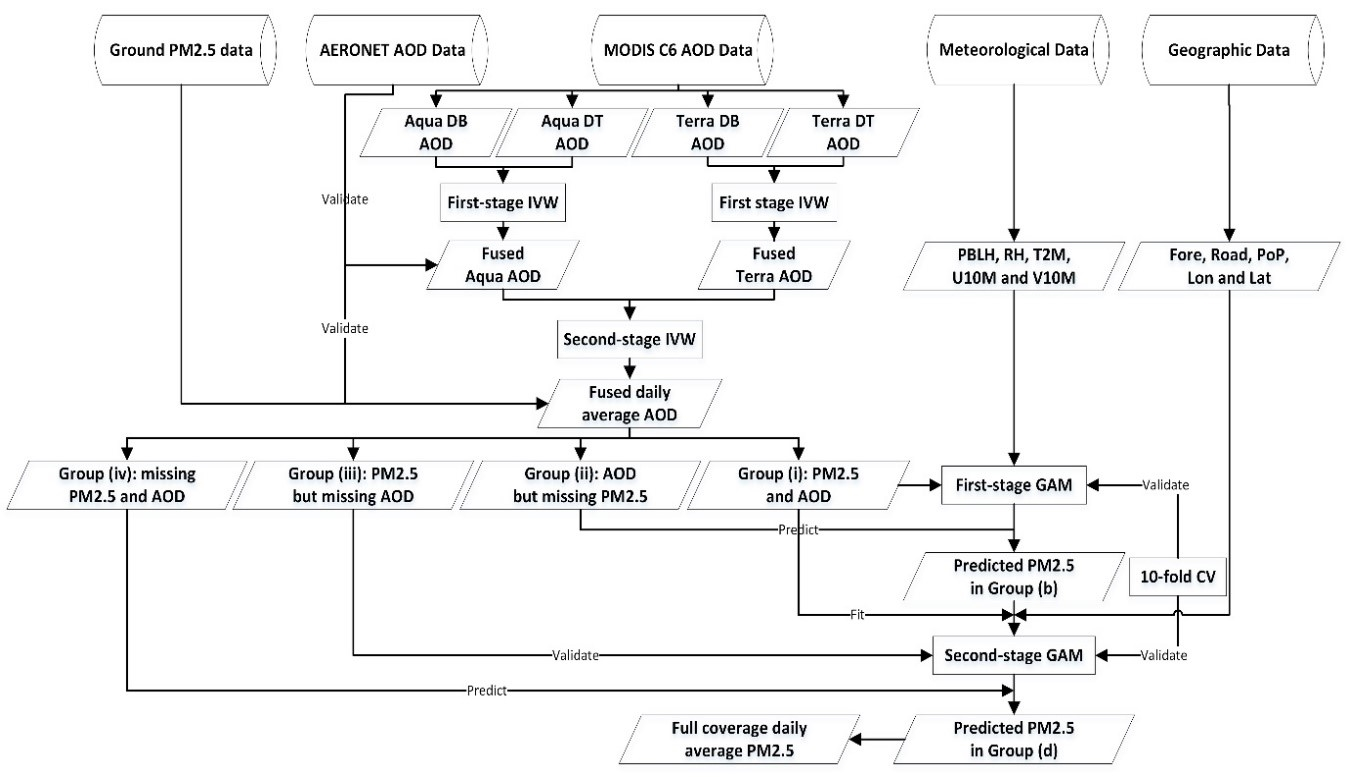
3.1. Fusing MODIS Terra and Aqua AOD via Two-Stage IVW

The original MODIS C6 AOD product has many missing pixels due to cloud contamination and other factors, which severely impacts the daily PM_2.5 retrievals and its further application. Fortunately, the MODIS Terra and Aqua satellites have the same revisiting period, same bands and a small difference in the passing time. Meanwhile, the DT AOD is made for a dark surface, and the second generation of DB AOD is created for both dark and bright surfaces. These produce strong spatial–temporal correlations between DB and DT AOD from two satellites in the same area, and provide a high probability of making spatial complementarity. On the other hand, the different data quality of AOD will greatly affect the fusion result, and accordingly the weights of AOD data accuracy should be incorporated into the procedure. Accordingly, we propose the two-stage IVW to fuse the four AOD products (Terra DB, Terra DT, Aqua DB and Aqua DT) and improve the spatial coverage of daily MODIS AOD product. The Two-stage IVW includes the following three steps.

(1) The DB and DT AOD products of Terra and Aqua with different QA (i.e., 1, 2, and 3) were evaluated by comparing them with the AERONET AOD. The data evaluation is to guarantee the proper input for the next step of fusion. In the procedure, several popular accuracy indicators are utilized, i.e., root mean square (RMSE), coefficient of determination (R²), relative percentage error (RPE) and expected error (EE). The EE is a deviation interval between MODIS C6 and AERONET AOD, and the interval in this study is manually set as 0.05 + 0.2 × AERONET AOD [59].

(2) The first stage of the IVW algorithm was implemented to fuse the DB and DT AOD data for both Terra and Aqua satellites separately. Taking the Terra satellite as an example, with over 10 pairs of evaluated daily MODIS Terra DT and DB AOD on the same grid cells, two linear regression equations can be separately formulated as [16]:

$${\tau }_{DT}={\beta }_1+{\alpha }_1\times {\tau }_{DB}$$

(1)

$${\tau }_{DB}={\beta }_2+{\alpha }_2\times {\tau }_{DT}$$

(2)

where ${\tau }_{DB}$ and ${\tau }_{DT}$ are daily Terra MODIS DB and DT AOD, respectively, ${\beta }_1$ and ${\beta }_2$ are intercepts of regression functions, respectively, and ${\alpha }_1$ and ${\alpha }_2$ are slopes, respectively. For the grid cells with DB AOD, Equation (1) is to predict and fill the missing DT AOD with the DB AOD; for the grid cells with DT AOD, Equation (2) is to fill the missing DB AOD with the DT AOD. The two equations are formulated using the linear correlations between DB AOD and DT AOD, but they could not simultaneously be used to predict the AOD on the same grid cells. After that, the filled DB AOD and DT AOD were compared with the AOD of its nearest AERONET sites. The standard variance of filled DB AOD and DT AOD within the same season shows the degree of deviation of the data from its expected values (i.e., AERONET AOD), and a larger variance indicates a worse data quality of the MODIS AOD. Accordingly, taking the variance reciprocals of MODIS DB and DT AOD as weights, the IVW fuses MODIS DB and DT AOD as:

$${\tau }_c=\frac{{\tau }_{DT\_f}/Va{r}_{DT}+{\tau }_{DB\_f}/Va{r}_{DB}}{1/Va{r}_{DT}+1/Va{r}_{DB}}$$

(3)

where ${\tau }_c$ is the IVW fused Terra daily AOD from DB and DT; ${\tau }_{DB\_f}$ and ${\tau }_{DT\_f}$ are filled DB and DT AOD using linear regressions in (1) and (2), respectively; $Va{r}_{DB}$ and $Va{r}_{DT}$ are the variances of DB and DT AOD against AERONET AOD in the same season, respectively.

(3) Following Step 2, the fused AOD data of Terra and Aqua was also fused with the IVW. The two linear regression functions between fused Terra AOD and Aqua AOD were separately formulated to predict and fill the missing Aqua AOD and Terra AOD in the same grid cells. After that, the weights of filled Aqua AOD and Terra AOD were computed by comparing with the nearest AERONET AOD. The daily average MODIS AOD was finally obtained by linearly fusing the filled Aqua and Terra AOD with the variance reciprocals as weights.

3.2. Retrieving PM_2.5 from Fused MODIS AOD and Two-Stage GAM

The above fusion procedures improved the spatial coverage of daily MODIS AOD, but could not accurately estimate all the missing AOD. The missing AOD still degrades the utility performance of PM_2.5 retrievals. The GAM could better consider nonlinear correlations between PM_2.5 concentrations and geographic and meteorological data. Therefore, we adopted the two-stage GAM model to retrieve the PM_2.5 concentrations and obtain full coverage PM_2.5 data in the study area. Among all the datasets, the PM_2.5 and AOD data had missing values, and accordingly we manually divided the two datasets in all the grid cells into four groups: (i) PM_2.5 and AOD; (ii) AOD but missing PM_2.5; (iii) PM_2.5 but missing AOD; and (iv) missing PM_2.5 and AOD. The two-stage GAM incorporates the following two procedures.

(1) Group (i) was used to model the first-stage GAM model and predict the PM_2.5 with the AOD in group (ii). Except the fused daily average AOD, the first-stage GAM utilizes meteorological data as auxiliary factors to reflect the time variability of PM_2.5 concentrations as:

$${\left(PM{2.5}_{GAM1}\right)}_{ij}={\mu }_0+f{\left(AOD\right)}_j+f{\left(PBLH\right)}_j+f{\left(RH\right)}_j+f{\left(T2M\right)}_j+f{\left(U10M,V10M\right)}_j+{\epsilon }_{ij}$$

(4)

where ${\left(PM{2.5}_{GAM1}\right)}_{ij}$ is the predicted average PM_2.5 in the grid cell j on the data i from the first-stage GAM; ${\mu }_0$ is the constant term; $f{\left(PBLH\right)}_j$, $f{\left(RH\right)}_j$, $f{\left(T2M\right)}_j$ and $f{\left(U10M,V10M\right)}_j$ are smooth functions of planetary boundary layer height, relative humidity, temperature at 2 m above the ground, and the wind speed and direction at 10 m above the ground in the grid cell j, respectively; and ${\epsilon }_{ij}$ is the residual error of grid cell j at data i.

(2) Group (i) and the predicted PM_2.5 in group (ii) were integrated with geographic data to model the second-stage GAM. In our study, the second-stage GAM adopts the smooth functions of population, forest coverage, road coverage and spatial locations as main factors to predict the spatial variability of PM_2.5 in group (iv). The second-stage GAM model was formulated as:

$${\left(PM{2.5}_{GAM2}\right)}_{ij}={\mu }_1+f{\left(Lon,Lat\right)}_j+f{\left(\log \left(Fore\right)\right)}_j+f{\left(\log (Road)\right)}_j+f{\left(\log \left(Pop\right)\right)}_j+{ϵ}_{ij}$$

(5)

where ${\left(PM{2.5}_{GAM2}\right)}_{ij}$ is the predicted average PM_2.5 in the grid cell j on the data i from the second-stage GAM; $f{\left(Lon,Lat\right)}_j$, $f{\left(\log \left(Fore\right)\right)}_j$, $f{\left(\log (Road)\right)}_j$ and $f{\left(\log \left(Pop\right)\right)}_j$ are smooth functions of spatial locations (i.e., longitude, latitude), forest coverage rate, road coverage rate and population density respectively; ${\mu }_1$ is the constant term and ${ϵ}_{ij}$ is residual error of grid cell j at data i.

3.3. Model Evaluation and Validation

In this study, we implemented two main schemes to evaluate the performance of both two-stage IVW in fusing daily MODIS AOD data and two-stage GAM in retrieving PM_2.5 concentrations. For the two-stage IVW, the fused daily average MODIS AOD was compared with its nearest AERONET AOD, and several popular indicators were used to quantify the accuracy, including RMSE, R², and RPE. Meanwhile, the spatial coverage rate (SCR) of fused daily average MODIS AOD was also computed and compared with those from the first-stage IVW and the original MODIS AOD product.

The performance of two-stage GAM was evaluated from its two stages separately. For the first-stage GAM, the ten-fold cross validation (10-fold CV) was utilized, and the adopted indicators were scatter plots of true and predicted PM_2.5, RMSE, R² and RPE. The modelling performance of second-stage GAM was assessed from three different aspects. The feasibility evaluation of geographic factors in the second-stage GAM was evaluated by modelling fitting with MODIS AOD and PM_2.5 data in group (i). Meanwhile, ten-fold CV was used to evaluate the second-stage GAM on the integration of group (i) and predicted PM_2.5 in group (ii). Moreover, the PM_2.5 in group (iii) was implemented as the ground truth to compare with the predicted PM_2.5 from two-stage GAM to further validate its performance.

4. Experimental Results

4.1. Experiments on Fused Daily Average MODIS AOD

4.1.1. Accuracy Evaluation of MODIS AOD from Two-Stage IVW

Table 2. The comparison in R² among MODIS standard AOD, fused AOD from first-stage IVW and fused daily average MODIS AOD from two-stage IVW.

Data	R2
	MODIS Standard AOD	Fused MODIS AOD from First-Stage IVW	Fused Daily Average MODIS AOD from Two-Stage IVW
Terra 2013	0.57	0.60	0.66
Aqua 2013	0.44	0.55
Terra 2014	0.74	0.60	0.64
Aqua 2014	0.66	0.74
Terra 2015	0.70	0.67	0.60
Aqua 2015	0.64	0.60
Terra 2016	0.64	0.56	0.68
Aqua 2016	0.64	0.58
Average	0.63	0.60	0.63

lists the R² of MODIS standard AOD, the fused MODIS Terra and Aqua AOD from first-stage IVW and the fused daily average MODIS AOD from second-stage IVW in the YRD in 2013–2016. The R² was estimated by comparing the above three AOD products with those of AERONET AOD sites. The first-stage IVW slightly lowers the accuracy of MODIS standard AOD, and the second-stage promotes the accuracy of fused MODIS Terra and Aqua AOD. The average accuracy of MODIS standard AOD during 2013–2016 did not change much after the two-stage IVW fusion.

4.1.2. The SCR Evaluation of MODIS AOD from Two-Stage IVW

Table 3. Comparison in spatial coverage rate (SCR) among MODIS standard AOD, fused daily AOD from first-stage IVW and from two-stage IVW.

Dataset	SCR
	MODIS Standard AOD	Fused MODIS AOD from First-Stage IVW	Fused Daily Average MODIS AOD from Two-Stage IVW
Terra 2013	15.95%	34.82%	45.84%
Aqua 2013	15.28%	34.81%
Terra 2014	12.27%	30.61%	40.90%
Aqua 2014	11.22%	29.77%
Terra 2015	10.44%	26.12%	35.17%
Aqua 2015	9.45%	25.86%
Terra 2016	11.07%	26.29%	35.23%
Aqua 2016	9.32%	25.27%
Average	11.88%	29.19%	39.29%

lists the spatial coverage rates of MODIS standard AOD, fused MODIS AOD from first-stage IVW and fused daily average MODIS AOD from two-stage IVW during 2013–2016. The average SCR of original MODIS standard AOD is as low as 11.88%, and the first-stage IVW greatly improves the spatial coverage rate of original MODIS AOD product up to 29.19%. Moreover, after the second-state IVW, the SCR of fused daily average MODIS AOD reaches up to 39.29%, and improves about 230% against the original MODIS AOD. Moreover, Figure 3 compares the annual coverage information of MODIS standard AOD and fused daily average MODIS AOD from two-stage IVW. The annual coverage days of MODIS AOD after two-stage IVW have been greatly promoted, particularly in the north region of YRD. The promotion of coverage days in Taihu Lake and coastal areas of south YRD is not obvious, and the explanation for that is their rain and cloudy weather easily reduce the effectiveness of MODIS AOD data.

4.2. Experiments on PM_2.5 Retrieved from Two-Stage GAM

This section explores the performance of two-stage GAM in retrieving full-coverage PM_2.5 in the YRD region during 2013–2016. We used the Pearson correlation on meteorological factors (T2M, PBLH, RH, V10M, U10M) and geographic factors (Pop, Fore, and Road) to avoid collinearity problems among them. All the above factors showed good independent statistical behaviors and were used in the experiments. The geographic data were transformed into logarithmic formats to alleviate their spatial homogeneity.

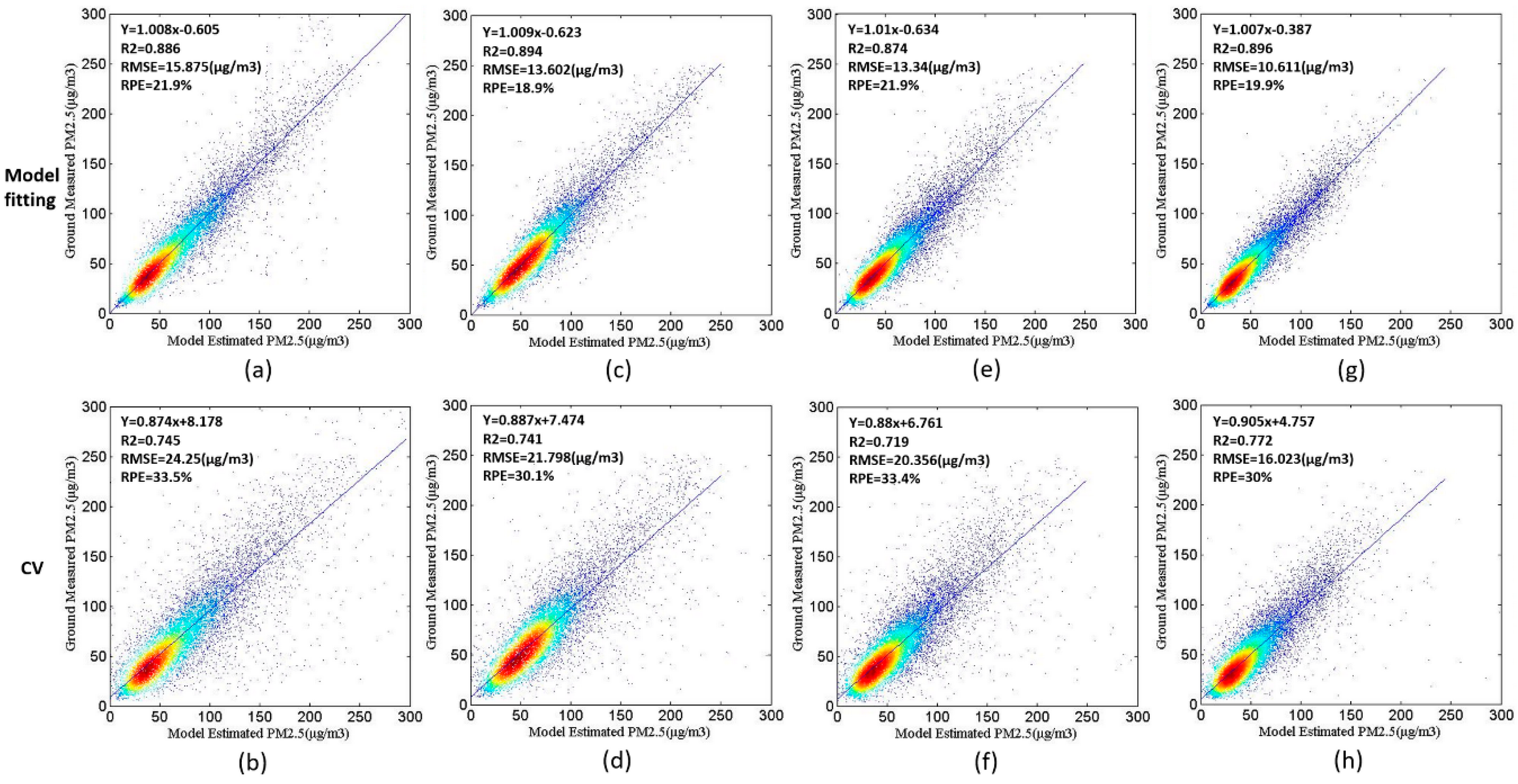
4.2.1. The Performance Verification of First-Stage GAM

Figure 4 depicts the regression results with zero intercept between our predicted PM_2.5 of group (i) against observed PM_2.5 measures using the 10-fold CV scheme in 2013–2016. The first-stage GAM showed slight overfitting throughout all the four years when compared with their model fitting results. Fortunately, the higher R², low RMSE and RPE proves the robustness and reliability of the model, and therefore we suggest the predicted PM_2.5 in group (ii) can be used in the second-stage GAM model.

4.2.2. The Performance Verification of Second-Stage GAM

Combing the data in groups (i) and (ii), we further implemented the PM_2.5 and fused MODIS AOD to verify the second-stage GAM model in Equation (5). Figure 5 shows the scatter plots between the predicted and observed PM_2.5 in groups (i)+(ii), where the predicted PM_2.5 of group (ii) in the first-stage GAM was utilized as the ground truth in this model. The results show the second-stage GAM model behaves well in model fitting and the 10-fold CV test, and no clear overfitting exists in the model. The explanation for this is the involvement of PM_2.5 in group (i) and the predicted PM_2.5 in group (ii) improves the robustness of the second-stage GAM model. Meanwhile, Figure 6 shows the scatter plots of predicted PM_2.5 from second-stage GAM and the observed PM_2.5 in group (iii). The high averaged R² = 0.78, low averaged RMSE = 19.177 μg/m³ and averaged RPE = 28.9% also support the above observations of the second-stage GAM model.

4.2.3. Comparison with Other Spatial Interpolation Methods

We further compared our full-coverage PM_2.5 concentration results with those of two widely used spatial interpolation methods; the inverse distance weighted method (IDW) and ordinary kriging (OK). IDW interpolates values at unknown grid cells using weighted known neighborhood PM_2.5 measures, and the weights are inversely proportional to the distance to the target grid cells. Different from other kriging approaches, the most commonly used OK estimates the unknow PM_2.5 on certain grid cells by using weighted linear combinations of the neighboring measures. We did not implement more complicated methods because there are too many prerequisites in essential datasets. For example, the multiple imputation model [52] by Xiao requires the atmospheric correction AOD with community multiscale air quality (CMAQ) simulations, whereas the parameters of CMAQ are unavailable for our study areas.

We then implemented the three methods on the ground observations to obtain full-coverage PM_2.5 in the YRD in 2013–2016. We benchmarked the performance of all three methods using five-fold cross validation. In detail, we randomly removed 20% of the ground stations and predicted their PM_2.5 concentrations as measured at the stations. Each model was trained using 80% of the ground PM_2.5 concentrations, and then tested on the remaining 20% of the observations.

Table 4. Geospatial prediction models evaluation.

Years	Models	Quantitative Measures
		MAPE	RMSE	RPE	R2
2013	IDW	35.510	23.210	34.46%	0.697
	OK	30.578	23.256	35.47%	0.757
	Ours	15.722	21.419	28.39%	0.806
2014	IDW	37.770	20.910	31.88%	0.658
	OK	30.484	25.206	34.88%	0.731
	Ours	20.523	23.212	31.15%	0.742
2015	IDW	37.608	18.170	32.78%	0.654
	OK	36.644	22.531	40.42%	0.671
	Ours	21.062	17.513	29.70%	0.778
2016	IDW	38.019	19.265	40.74%	0.673
	OK	35.436	18.886	39.72%	0.707
	Ours	19.097	17.416	32.70%	0.733

lists the comparison results of all three methods, where RMSE, RPE, R² and mean absolute percentage error (MAPE) were used to quantify the differences between retrieved PM_2.5 concentrations and ground observations. Our method performed the best, achieving the largest R² and the smallest MAPE and RPE, particularly in the year 2013.

5. Discussion

The above three experiments comprehensively investigated the performance of our proposed framework in the retrieval of full-coverage daily average PM_2.5 during 2013–2016. The first experiment verifies the accuracy and SCR of fused daily average MODIS AOD from two-stage IVW. Experimental results show that the R² of fused daily average MODIS AOD offers no clear difference from the original MODIS standard AOD product, but the SCR (i.e., spatial coverage rate) was greatly improved by 230% when compared with the original MODIS AOD. Therefore, the two-stage IVW could satisfy the fusing requirements of MODIS DB and DT AOD from Terra and Aqua satellites and yield high-coverage daily average MODIS AOD data.

The fused daily average MODIS AOD and ground PM_2.5 were classified into four groups, and the two-stage GAM were designed to retrieve the ground PM_2.5 in group (ii) and (iv) to obtain full-coverage daily average PM_2.5 in the YRD region. The data in group (i) was used to model the first- stage GAM to predict the ground PM_2.5 in group (ii). The accuracy evaluation result in the first-stage GAM shows that the predicted PM_2.5 in group (i) has high R², low RMSE and RPE and could satisfy the practical requirements in predicting that of group (ii). The performance of second-stage GAM was evaluated by comparing the predicted PM_2.5 in groups (i) and (ii) with the observed, where the predicted PM_2.5 in group (ii) in the first-stage GAM was regarded as the observed in the second-stage GAM. Experimental results show that the second-stage GAM model behaves well, with no clear overfitting, but a higher accuracy makes it useful in predicting PM_2.5 in group (iv). Meanwhile, the accuracy evaluation of second-stage GAM on the data in group (iii) also supports the above observations. The two-stage GAM model has good performance in retrieving the ground PM_2.5 in groups (ii) and (iv), and the full-coverage daily average PM_2.5 can be obtained via the combination of the above results.

The third experiment compared the performance of our methods with two widely used spatial interpolation methods IDW and OK. The observations show that all three methods could obtain full-coverage PM_2.5 concentration maps, but our retrieved results are superior to those of IDW and OK. This verifies the advantages of combining satellite AOD and ground-observed PM_2.5 concentrations against the single data source of ground measures in mapping full-coverage PM_2.5 concentrations, which coincides with previous studies [46,52]. The IDW and OK methods highly rely on the spatial distributions of ground stations, and the sparse or nonexistent PM_2.5 measures in the YRD would negatively affect the estimated full-coverage map. In contrast, the implemented GAM models in our presented framework could describe the spatial inference of PM_2.5 concentrations well, and accordingly perform better than IDW and OK.

Unfortunately, our study has some limitations. The first is regarding the data quality of MODIS DB/DT AOD. We used the MODIS standard AOD with QA = 1, 2 and 3 in the two-stage IVW model to ensure sufficient AOD data. The poor data quality of QA = 2 and 3 negatively affects the fusion procedure and may make the two-stage IVW ineffective in improving the accuracy of daily average MODIS AOD. The AOD with good quality, with QA = 1, in long series, will be implemented to obtain daily average MODIS AOD with a higher accuracy. The second is regarding the selection of meteorological and geographic factors in the two-stage GAM model. In our experiment, we followed previous studies, selected the most popular factors and did not carefully analyze the specific characteristic of the YRD region. The future work will involve more meteorological and geographic factors. The third is that we only implemented the MODIS C6 AOD product, which might not capture the variability of daily PM_2.5 distribution on the intra-urban scale. The newly released MODIS MAIAC AOD [60,61,62] with 1 km spatial resolution will be used to further investigate the performance of our framework. The fourth is that we only compared our proposed framework with the IDW and OK. More state-of-the-art full-coverage PM_2.5 concentrations like machine learning models [49,50,51] will be used to make comparisons with our method on much larger study areas, e.g., the whole of China or the whole continent.

6. Conclusions

Satellite-based remote sensing techniques have been widely used in mapping PM_2.5 concentrations in the YRD region, particularly using the MODIS AOD product. However, current PM_2.5 concentrations retrieved from the MODIS AOD product have severe missing data, and cannot obtain a full-coverage PM_2.5 concentration map. This severely degrades its utility performance in many realistic applications. This paper proposes an innovative framework to retrieve full-coverage daily average PM_2.5 from the MODIS C6 AOD product. The two-stage IVW algorithm was utilized to fuse MODIS DB and DT AOD from Terra and Aqua satellites. This greatly improves the coverage rate of the MODIS AOD product. After that, the two-stage GAM model was employed to retrieve ground PM_2.5 concentrations from the fused daily average MODIS AOD data, and the full-coverage daily PM_2.5 map was finally achieved. Using the MODIS AOD data from 2013–2016, two groups of experiments were carefully designed in order to comprehensively testify the performances of our proposed framework in both fusing MODIS AOD and retrieving full-coverage PM_2.5. Experimental results show that the two-stage IVW could improve spatial coverage of MODIS AOD against the original standard product by 230%, meanwhile maintaining the data accuracy of MODIS AOD data. The average spatial coverage ratio of daily MODIS AOD in 2013–2016 of YRD reaches up to 39.29% after the fusion operation of second-state IVW. The annual coverage days of MODIS AOD after two-stage IVW has been clearly improved, especially in the north of the YRD region. Moreover, the experiments on two-stage GAM show that the first-stage GAM can predict the ground PM_2.5 of group (ii) (i.e., AOD but missing PM_2.5) well, with slight overfitting throughout the years of 2013–2016. That explains the robustness and reliability of the first-stage GAM model. Meanwhile, experimental results show that the second-stage GAM predicts the PM_2.5 concentrations in groups (iii) (PM_2.5 but missing AOD) and (iv) (i.e., missing PM_2.5 and AOD) well. Furthermore, we compared our framework with two widely used spatial interpolation methods, i.e., IDW and OK, in mapping the full-coverage daily PM_2.5 concentrations. The results show that our retrieved full-coverage PM_2.5 result has higher accuracies than those of IDW and OK, achieving the largest R² and the smallest MAPE and RPE in the year of 2013. Therefore, our proposed framework provides a good methodology for mapping full-coverage daily average PM_2.5 from the MODIS AOD product.

References

1. Zhang, Q.; He, K.; Huo, H. Policy: Cleaning China’s air. Nature 2012, 484, 161–162. [Google Scholar] [CrossRef] [PubMed]
2. Huang, R.-J.; Zhang, Y.; Bozzetti, C.; Ho, K.-F.; Cao, J.-J.; Han, Y.; Daellenbach, K.R.; Slowik, J.G.; Platt, S.M.; Canonaco, F.; et al. High secondary aerosol contribution to particulate pollution during haze events in China. Nature 2014, 514, 218–222. [Google Scholar] [CrossRef] [Green Version]
3. Wang, H.; Zhang, Y.; Zhao, H.; Lu, X.; Zhang, Y.; Zhu, W.; Nielsen, C.P.; Li, X.; Zhang, Q.; Bi, J. Trade-driven relocation of air pollution and health impacts in China. Nat. Commun. 2017, 8, 738. [Google Scholar] [CrossRef] [PubMed]
4. Zhang, Y.; Ding, A.; Mao, H.; Nie, W.; Zhou, D.; Liu, L.; Huang, X.; Fu, C. Impact of synoptic weather patterns and inter-decadal climate variability on air quality in the north China plain during 1980–2013. Atmos. Environ. 2016, 124, 119–128. [Google Scholar] [CrossRef]
5. Hu, X.-M.; Ma, Z.; Lin, W.; Zhang, H.; Hu, J.; Wang, Y.; Xu, X.; Fuentes, J.D.; Xue, M. Impact of the loess plateau on the atmospheric boundary layer structure and air quality in the north China plain: A case study. Sci. Total Environ. 2014, 499, 228–237. [Google Scholar] [CrossRef] [PubMed]
6. Wang, T.; Jiang, F.; Deng, J.; Shen, Y.; Fu, Q.; Wang, Q.; Fu, Y.; Xu, J.; Zhang, D. Urban air quality and regional haze weather forecast for yangtze river delta region. Atmos. Environ. 2012, 58, 70–83. [Google Scholar] [CrossRef]
7. She, Q.; Peng, X.; Xu, Q.; Long, L.; Wei, N.; Liu, M.; Jia, W.; Zhou, T.; Han, J.; Xiang, W. Air quality and its response to satellite-derived urban form in the yangtze river delta, China. Ecol. Indic. 2017, 75, 297–306. [Google Scholar] [CrossRef]
8. Zhong, L.; Louie, P.K.; Zheng, J.; Yuan, Z.; Yue, D.; Ho, J.W.; Lau, A.K. Science–policy interplay: Air quality management in the pearl river delta region and Hong Kong. Atmos. Environ. 2013, 76, 3–10. [Google Scholar] [CrossRef]
9. Huang, Y.; Deng, T.; Li, Z.; Wang, N.; Yin, C.; Wang, S.; Fan, S. Numerical simulations for the sources apportionment and control strategies of PM2.5 over pearl river delta, China, part i: Inventory and PM2.5 sources apportionment. Sci. Total Environ. 2018, 634, 1631–1644. [Google Scholar] [CrossRef]
10. Guan, D.; Su, X.; Zhang, Q.; Peters, G.P.; Liu, Z.; Lei, Y.; He, K. The socioeconomic drivers of China’s primary PM2.5 emissions. Environ. Res. Lett. 2014, 9, 024010. [Google Scholar] [CrossRef]
11. Han, L.; Zhou, W.; Li, W.; Li, L. Impact of urbanization level on urban air quality: A case of fine particles (PM2.5) in Chinese cities. Environ. Pollut. 2014, 194, 163–170. [Google Scholar] [CrossRef] [PubMed]
12. Hao, Y.; Liu, Y.-M. The influential factors of urban PM2.5 concentrations in China: A spatial econometric analysis. J. Clean. Prod. 2016, 112, 1443–1453. [Google Scholar] [CrossRef]
13. Xing, Y.-F.; Xu, Y.-H.; Shi, M.-H.; Lian, Y.-X. The impact of PM2.5 on the human respiratory system. J. Thorac. Dis. 2016, 8, E69. [Google Scholar] [PubMed]
14. Ma, Z.; Hu, X.; Sayer, A.M.; Levy, R.; Zhang, Q.; Xue, Y.; Tong, S.; Bi, J.; Huang, L.; Liu, Y. Satellite-based spatiotemporal trends in PM2.5 concentrations: China, 2004–2013. Environ. Health Perspect. 2016, 124, 184–192. [Google Scholar] [CrossRef] [PubMed]
15. Song, Z.; Fu, D.; Zhang, X.; Han, X.; Song, J.; Zhang, J.; Wang, J.; Xia, X. MODIS AOD sampling rate and its effect on PM2. 5 estimation in North China. Atmos. Environ. 2019, 209, 14–22. [Google Scholar] [CrossRef]
16. Ma, Z.; Hu, X.; Huang, L.; Bi, J.; Liu, Y. Estimating ground-level PM2.5 in China using satellite remote sensing. Environ. Sci. Technol. 2014, 48, 7436–7444. [Google Scholar] [CrossRef] [PubMed]
17. Liu, Y.; Franklin, M.; Kahn, R.; Koutrakis, P. Using aerosol optical thickness to predict ground-level PM2.5 concentrations in the st. Louis area: A comparison between misr and modis. Remote Sens. Environ. 2007, 107, 33–44. [Google Scholar] [CrossRef]
18. Sorek-Hamer, M.; Kloog, I.; Koutrakis, P.; Strawa, A.W.; Chatfield, R.; Cohen, A.; Ridgway, W.L.; Broday, D.M. Assessment of PM2.5 concentrations over bright surfaces using modis satellite observations. Remote Sens. Environ. 2015, 163, 180–185. [Google Scholar] [CrossRef]
19. Xie, Y.; Wang, Y.; Zhang, K.; Dong, W.; Lv, B.; Bai, Y. Daily estimation of ground-level PM2.5 concentrations over beijing using 3 km resolution modis aod. Environ. Sci. Technol. 2015, 49, 12280–12288. [Google Scholar] [CrossRef]
20. Lee, H.J.; Chatfield, R.B.; Strawa, A.W. Enhancing the applicability of satellite remote sensing for PM2.5 estimation using modis deep blue aod and land use regression in California, United States. Environ. Sci. Technol. 2016, 50, 6546–6555. [Google Scholar] [CrossRef]
21. Chu, D.; Kaufman, Y.; Ichoku, C.; Remer, L.; Tanré, D.; Holben, B. Validation of modis aerosol optical depth retrieval over land. Geophys. Res. Lett. 2002, 29, MOD2-1–MOD2-4. [Google Scholar] [CrossRef]
22. Sayer, A.; Hsu, N.; Bettenhausen, C.; Jeong, M.J. Validation and uncertainty estimates for modis collection 6 “deep blue” aerosol data. J. Geophys. Res. Atmos. 2013, 118, 7864–7872. [Google Scholar] [CrossRef]
23. Wei, J.; Sun, L. Comparison and evaluation of different modis aerosol optical depth products over the Beijing-Tianjin-Hebei region in China. IEEE J. Sel. Top. Appl. Earth Obs. Remote Sens. 2017, 10, 835–844. [Google Scholar] [CrossRef]
24. Van Donkelaar, A.; Martin, R.V.; Park, R.J. Estimating ground-level PM2.5 using aerosol optical depth determined from satellite remote sensing. J. Geophys. Res. Atmos. 2006, 111, D21201–D21210. [Google Scholar] [CrossRef]
25. Jiang, M.; Sun, W.; Yang, G.; Zhang, D. Modelling seasonal gwr of daily PM2.5 with proper auxiliary variables for the yangtze river delta. Remote Sens. 2017, 9, 346. [Google Scholar] [CrossRef]
26. Liu, Y.; Park, R.J.; Jacob, D.J.; Li, Q.; Kilaru, V.; Sarnat, J.A. Mapping annual mean ground-level PM2.5 concentrations using multiangle imaging spectroradiometer aerosol optical thickness over the contiguous united states. J. Geophys. Res. Atmos. 2004, 109, D22206–D22215. [Google Scholar]
27. Boys, B.; Martin, R.; Van Donkelaar, A.; MacDonell, R.; Hsu, N.; Cooper, M.; Yantosca, R.; Lu, Z.; Streets, D.; Zhang, Q.; et al. Fifteen-year global time series of satellite-derived fine particulate matter. Environ. Sci. Technol. 2014, 48, 11109–11118. [Google Scholar] [CrossRef]
28. Zhang, Y.; Li, Z. Remote sensing of atmospheric fine particulate matter (PM2.5) mass concentration near the ground from satellite observation. Remote Sens. Environ. 2015, 160, 252–262. [Google Scholar] [CrossRef]
29. Ma, Z. Study on Spatiotemporal Distribution of PM2.5 in China Using Satellite Remote Sensing. Ph.D. Thesis, Nanjing University, Nanjing, China, 2015; pp. 8–52. [Google Scholar]
30. Li, Z.; Zhang, Y.; Shao, J.; Li, B.; Hong, J.; Liu, D.; Li, D.; Wei, P.; Li, W.; Li, L. Remote sensing of atmospheric particulate mass of dry PM2.5 near the ground: Method validation using ground-based measurements. Remote Sens. Environ. 2016, 173, 59–68. [Google Scholar] [CrossRef]
31. Chen, G.; Guang, J.; Xue, Y.; Li, Y.; Che, Y.; Gong, S. A physically based PM2.5 estimation method using aeronet data in beijing area. IEEE J. Sel. Top. Appl. Earth Obs. Remote Sens. 2018, 11, 1957–1965. [Google Scholar] [CrossRef]
32. Lin, C.; Li, Y.; Yuan, Z.; Lau, A.K.H.; Li, C.; Fung, J.C.H. Using satellite remote sensing data to estimate the high-resolution distribution of ground-level PM2.5. Remote Sens. Environ. 2015, 156, 117–128. [Google Scholar] [CrossRef]
33. Tian, J.; Chen, D. A semi-empirical model for predicting hourly ground-level fine particulate matter (PM2.5) concentration in southern ontario from satellite remote sensing and ground-based meteorological measurements. Remote Sens. Environ. 2010, 114, 221–229. [Google Scholar] [CrossRef]
34. You, W.; Zang, Z.; Zhang, L.; Li, Z.; Chen, D.; Zhang, G. Estimating ground-level PM10 concentration in northwestern China using geographically weighted regression based on satellite aod combined with calipso and modis fire count. Remote. Sens. Environ. 2015, 168, 276–285. [Google Scholar] [CrossRef]
35. Zou, B.; Pu, Q.; Bilal, M.; Weng, Q.; Zhai, L.; Nichol, J.E. High-resolution satellite mapping of fine particulates based on geographically weighted regression. IEEE Geosci. Remote Sens. Lett. 2016, 13, 495–499. [Google Scholar] [CrossRef]
36. Ma, Z.; Liu, Y.; Zhao, Q.; Liu, M.; Zhou, Y.; Bi, J. Satellite-derived high resolution PM2.5 concentrations in yangtze river delta region of China using improved linear mixed effects model. Atmos. Environ. 2016, 133, 156–164. [Google Scholar] [CrossRef]
37. Bai, Y.; Wu, L.; Qin, K.; Zhang, Y.; Shen, Y.; Zhou, Y. A geographically and temporally weighted regression model for ground-level PM2.5 estimation from satellite-derived 500 m resolution aod. Remote Sens. 2016, 8, 262. [Google Scholar] [CrossRef]
38. Meng, X.; Garay, M.J.; Diner, D.J.; Kalashnikova, O.V.; Xu, J.; Liu, Y. Estimating PM2.5 speciation concentrations using prototype 4.4 km-resolution misr aerosol properties over southern California. Atmos. Environ. 2018, 181, 70–81. [Google Scholar] [CrossRef] [PubMed]
39. Van Donkelaar, A.; Martin, R.V.; Spurr, R.J.; Burnett, R.T. High-resolution satellite-derived PM2.5 from optimal estimation and geographically weighted regression over north America. Environ. Sci. Technol. 2015, 49, 10482–10491. [Google Scholar] [CrossRef]
40. Crouse, D.L.; Peters, P.A.; Hystad, P.; Brook, J.R.; van Donkelaar, A.; Martin, R.V.; Villeneuve, P.J.; Jerrett, M.; Goldberg, M.S.; Pope, C.A., III. Ambient PM2.5, O3, and NO2 exposures and associations with mortality over 16 years of follow-up in the Canadian census health and environment cohort (canchec). Environ. Health Perspect. 2015, 123, 1180–1186. [Google Scholar] [CrossRef]
41. De Hoogh, K.; Héritier, H.; Stafoggia, M.; Künzli, N.; Kloog, I. Modelling daily PM2.5 concentrations at high spatio-temporal resolution across Switzerland. Environ. Pollut. 2018, 233, 1147–1154. [Google Scholar] [CrossRef]
42. Just, A.C.; De Carli, M.M.; Shtein, A.; Dorman, M.; Lyapustin, A.; Kloog, I. Correcting measurement error in satellite aerosol optical depth with machine learning for modeling PM2.5 in the northeastern USA. Remote Sens. 2018, 10, 803. [Google Scholar] [CrossRef]
43. Smith, R.L.; Kolenikov, S.; Cox, L.H. Spatiotemporal modeling of PM2.5 data with missing values. J. Geophys. Res. Atmos. 2003, 108, 9004–9014. [Google Scholar] [CrossRef]
44. Van Donkelaar, A.; Martin, R.V.; Pasch, A.N.; Szykman, J.J.; Zhang, L.; Wang, Y.X.; Chen, D. Improving the accuracy of daily satellite-derived ground-level fine aerosol concentration estimates for north America. Environ. Sci. Technol. 2012, 46, 11971–11978. [Google Scholar] [CrossRef]
45. Zheng, Y.; Zhang, Q.; Liu, Y.; Geng, G.; He, K. Estimating ground-level PM2.5 concentrations over three megalopolises in China using satellite-derived aerosol optical depth measurements. Atmos. Environ. 2016, 124, 232–242. [Google Scholar] [CrossRef]
46. Tang, M.; Wu, X.; Agrawal, P.; Pongpaichet, S.; Jain, R. Integration of diverse data sources for spatial PM2.5 data interpolation. IEEE. Trans. Multimed. 2017, 19, 408–417. [Google Scholar] [CrossRef]
47. Bi, J.; Belle, J.H.; Wang, Y.; Lyapustin, A.I.; Wildani, A.; Liu, Y. Impacts of snow and cloud covers on satellite-derived PM2.5 levels. Remote Sens. Environ. 2019, 221, 665–674. [Google Scholar] [CrossRef]
48. Hu, H.; Hu, Z.; Zhong, K.; Xu, J.; Zhang, F.; Zhao, Y.; Wu, P. Satellite-based high-resolution mapping of ground-level PM2.5 concentrations over east China using a spatiotemporal regression kriging model. Sci. Total Environ. 2019, 672, 479–490. [Google Scholar] [CrossRef]
49. Zhao, C.; Liu, Z.; Wang, Q.; Ban, J.; Chen, N.X.; Li, T. High-resolution daily aod estimated to full coverage using the random forest model approach in the Beijing-Tianjin-Hebei region. Atmos. Environ. 2019, 203, 70–78. [Google Scholar] [CrossRef]
50. Vu, B.; Sánchez, O.; Bi, J.; Xiao, Q.; Hansel, N.; Checkley, W.; Gonzales, G.; Steenland, K.; Liu, Y. Developing an advanced PM2.5 exposure model in lima, Peru. Remote Sens. 2019, 11, 641. [Google Scholar] [CrossRef]
51. Xue, T.; Zheng, Y.; Tong, D.; Zheng, B.; Li, X.; Zhu, T.; Zhang, Q. Spatiotemporal continuous estimates of PM2.5 concentrations in China, 2000–2016: A machine learning method with inputs from satellites, chemical transport model, and ground observations. Environ. Int. 2019, 123, 345–357. [Google Scholar] [CrossRef]
52. Xiao, Q.; Wang, Y.; Chang, H.H.; Meng, X.; Geng, G.; Lyapustin, A.; Liu, Y. Full-coverage high-resolution daily PM2.5 estimation using MAIAC AOD in the Yangtze river Delta of China. Remote Sens. Environ. 2017, 199, 437–446. [Google Scholar] [CrossRef]
53. Laden, F.; Neas, L.M.; Dockery, D.W.; Schwartz, J. Association of fine particulate matter from different sources with daily mortality in six us cities. Environ. Health Perspect. 2000, 108, 941–947. [Google Scholar] [CrossRef]
54. Liu, Y.; Paciorek, C.J.; Koutrakis, P. Estimating regional spatial and temporal variability of PM2.5 concentrations using satellite data, meteorology, and land use information. Environ. Health Perspect. 2009, 117, 886–892. [Google Scholar] [CrossRef]
55. Remer, L.A.; Kaufman, Y.; Tanré, D.; Mattoo, S.; Chu, D.; Martins, J.V.; Li, R.-R.; Ichoku, C.; Levy, R.; Kleidman, R. The modis aerosol algorithm, products, and validation. J. Atmos. Sci. 2005, 62, 947–973. [Google Scholar] [CrossRef]
56. Bilal, M.; Nichol, J.E.; Nazeer, M. Validation of aqua-modis c051 and c006 operational aerosol products using aeronet measurements over pakistan. IEEE J. Sel. Top. Appl. Earth Obs. Remote Sens. 2016, 9, 2074–2080. [Google Scholar] [CrossRef]
57. Zhang, H.; Hoff, R.M.; Engel-Cox, J.A. The relation between moderate resolution imaging spectroradiometer (modis) aerosol optical depth and PM2.5 over the united states: A geographical comparison by us environmental protection agency regions. J. Air Waste Manag. Assoc. 2009, 59, 1358–1369. [Google Scholar] [CrossRef]
58. Lee, M.; Kloog, I.; Chudnovsky, A.; Lyapustin, A.; Wang, Y.; Melly, S.; Coull, B.; Koutrakis, P.; Schwartz, J. Spatiotemporal prediction of fine particulate matter using high-resolution satellite images in the southeastern us 2003–2011. J. Expo. Sci. Environ. Epidemiol. 2016, 26, 377–384. [Google Scholar] [CrossRef]
59. Nichol, J.; Bilal, M. Validation of modis 3 km resolution aerosol optical depth retrievals over Asia. Remote Sens. 2016, 8, 328. [Google Scholar] [CrossRef]
60. Lyapustin, A.; Martonchik, J.; Wang, Y.; Laszlo, I.; Korkin, S. Multiangle implementation of atmospheric correction (MAIAC): 1. Radiative transfer basis and look-up tables. J. Geophys. Res. Atmos. 2011, 116, D03210–D03218. [Google Scholar] [CrossRef]
61. Lyapustin, A.; Wang, Y.; Laszlo, I.; Kahn, R.; Korkin, S.; Remer, L.; Levy, R.; Reid, J. Multiangle implementation of atmospheric correction (MAIAC): 2. Aerosol algorithm. J. Geophys. Res. Atmos. 2011, 116, D03211–D03225. [Google Scholar] [CrossRef]
62. Kloog, I.; Sorek-Hamer, M.; Lyapustin, A.; Coull, B.; Wang, Y.; Just, A.C.; Schwartz, J.; Broday, D.M. Estimating daily PM2.5 and PM10 across the complex geo-climate region of Israel using MAIAC satellite-based AOD data. Atmos. Environ. 2015, 122, 409–416. [Google Scholar] [CrossRef]
Figure 1. Study area and distribution of ground-level PM2.5 and AERONET monitoring sites.
Remotesensing 11 01558 g001
Figure 2. The work flow of our methodology.
Remotesensing 11 01558 g002
Figure 3. Annual coverage days of MODIS standard AOD product and fused daily average AOD from two-stage IVW in the YRD during 2013–2016 (a,c,e,g): the MODIS standard AOD; (b,d,f,h): the fused daily average AOD from two-stage IVW.
Remotesensing 11 01558 g003
Figure 4. The accuracy evaluation of predicted PM2.5 in group (i) from the first-stage GAM model. (a,b): 2013; (c,d): 2014; (e,f): 2015; (g,h): 2016. The red lines are regression lines.
Remotesensing 11 01558 g004
Figure 5. The accuracy evaluation of the second-stage GAM model on groups (i)+(ii). (a,b): 2013; (c,d): 2014; (e,f): 2015; and (g,h): 2016. The red lines are regression lines.
Remotesensing 11 01558 g005
Figure 6. The accuracy evaluation of predicted PM2.5 in group (iii) from the second-stage GAM model. (a): 2013; (b): 2014; (c): 2015; and (d): 2016. The red lines are regression lines.
Remotesensing 11 01558 g006