A Novel Method for Estimating the Vertical Velocity of Air with a Descending Radiosonde System

Abstract

Knowledge of vertical air motion in the atmosphere is important for both meteorological and climate studies due to its impact on clouds, precipitation and the vertical transport of air masses, heat, momentum, and composition. The vertical velocity (VV) of air is among the most difficult and uncertain quantities to measure due to its generally small magnitude and high temporal and spatial variability. In this study, a descending radiosonde system is developed to derive VV at the low and middle troposphere in north China during the summer months. The VV is estimated from the difference between the observed radiosonde descent speed and the calculated radiosonde descent speed in still air based on the fluid dynamic principle. The results showed that the estimated VV generally ranged from −1 m/s to 1 m/s, accounting for 80.2% of data points. In convective conditions, a wider distribution of the VV was observed, which was skewed to large values relative to those in nonconvective conditions. The average VV throughout the entire profile was close to 0 m/s under nonconvective conditions. In contrast, distinctive vertical air motions below 5 km above the ground were recorded under convective activities. Vigorous air motions with an absolute VV >2 m/s were occasionally observed and were often associated with the occurrence of cloud layers. Moreover, the detailed structure of the instant air motion near the cloud boundaries (i.e., top and base), with an absolute VV >10 m/s in convective weather systems, was clearly revealed by this technique. The uncertainty estimation indicated that this method has the potential to capture and describe events with vertical air motions >0.69 m/s, which is useful for a convective weather study. Further studies are required to carefully assess the accuracy and precision of this novel VV estimation technique.

1. Introduction

Vertical air motion reflects dynamic processes in the atmosphere and is crucial for cloud diagnostics, numerical simulation validations [1], and investigations of the indirect effects of aerosols [2,3]. Moreover, vertical air velocity can influence the locations of activated cloud droplets that originate at the cloud top and base; therefore, it can affect cloud formation [4,5]. Previous studies have suggested that vertical air motion associated with anvil clouds played crucial roles in the mass and heat budgets of intense tropical convection systems [6]. The vertical velocity (VV) of air spanned a wide range of scales, from a very small turbulent motion (an order of 0.1 cm s⁻¹) to strong updrafts of ~15 m s⁻¹ in hurricane rainbands [7]. By conducting an overview of the parameterization of the gravity wave drag in numerical weather predictions and climate simulation models, Kim [8] demonstrated a close relationship between VV and the propagation, evolution and dissipation of gravity waves.

Despite its significance, VV is unfortunately among the most difficult and uncertain quantities to measure [9]. Large-scale velocity is typically small in magnitude but uniform and long-lasting. In contrast, a turbulent updraft is sometimes large but is randomly distributed with a short lifetime. Even in the conditions of moderate and strong convective systems, with a VV as large as several or even tens of m s⁻¹, this parameter is not easy to measure because of its random occurrence. The VV can be derived from the in situ measurements by towers and aircraft [10,11,12] and remotely measured using a ground-based Doppler radar/lidar [13,14,15,16,17,18]. Significant progress has recently been made on the satellite-based estimation of the vertical air motion either by quantifying the turbulent energy [19,20,21] or by tracking the vertical development of convective cloud tops [22].

Although those detecting approaches can provide valuable information pertaining to air vertical motion, more in situ VV measurements are still required. Considering that the balloon sounding lifting speed, which is calculated from its altitude information, is closely related to the air vertical motion, radiosonde and dropsonde may provide a potential method to estimate the air vertical motion [23,24,25,26]. Previous studies investigated atmospheric waves by analyzing the radiosonde ascent speed [27,28]. Radiosonde measurements could be used to determine the height of the boundary layer, since a dramatic decrease in the ascending speed would be expected at the top of this layer [29]; the balloon ascent speed was potentially a good indication of the atmospheric turbulence. Wang [30] indicated that strong vertical motions (larger than 1 m s⁻¹) could be captured via balloon sounding.

The dropsonde, which can provide in situ atmospheric profiles of the temperature, pressure, relative humidity (RH), wind speed and direction [31], was initially developed to study the vertical profiles of the kinematic and thermodynamic structure over vast seas and in severe weather conditions, such as hurricanes and typhoons [24,32]. Radiosondes, in contrast, are more available, as they have long been operationally released several times every day at radiosonde stations across the world. It is suggested that a dropsonde’s fall rate is much smoother than a radiosonde’s ascent rate [30] due to the radiosonde’s pendulum effect and the self-induced balloon motion [33], implying that the dropsonde-based VV estimations are more reliable than the radiosonde-based ones. This motivated us to add a dropsonde function based on the operational radiosondes. This is achieved by adding a cutter and a hard ball to the conventional radiosonde package. A field campaign was performed to test the system in north China during the summer months, and an estimation of the VV from this system was investigated in this study.

This paper is organized as follows. The main concept underlying the descending radiosonde system is described in Section 2. Section 3 introduces the site, data, and methodology. The error analysis and credibility assessment are presented in Section 4, followed by a discussion and summary in Section 5.

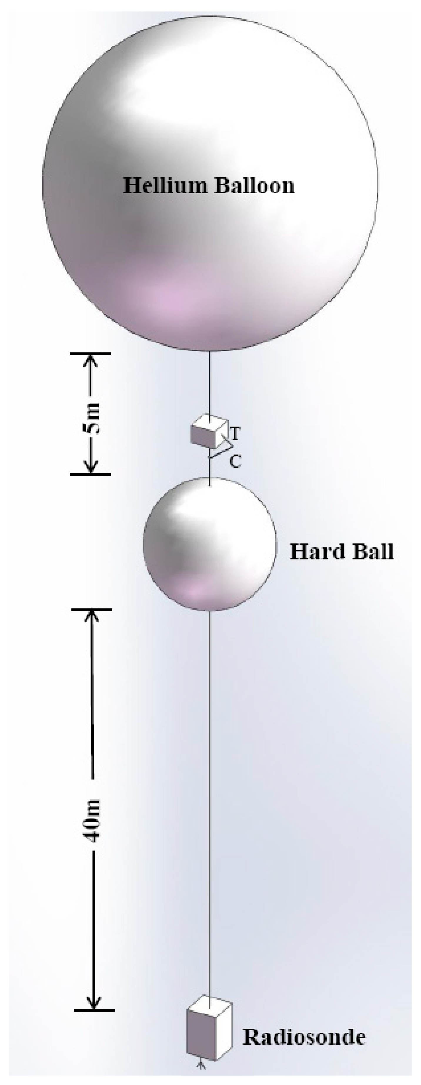
2. The Concept of the Descending Radiosonde System

The descending radiosonde system is developed based on a conventional radiosonde operated at upper air observation stations. Figure 1 shows a schematic diagram of the descending radiosonde system. It is mainly composed of a radiosonde and a 50 cm diameter hard ball that acts as the parachute. A cutter triggered by a timer is placed on a 5 m string, which links the balloon and the hard ball. The radiosonde hangs under the hard ball using a string 40 m in length. The string between the balloon and hard ball is cut when the instrument package is elevated to the upper troposphere by the balloon. Then, the radiosonde and hard ball begin to fall, while the balloon and cutter continue rising until the balloon bursts.

The hard ball is made of plastic foam with a weight of ~320 g. The conventional parachute used for the radiosonde is generally made of soft materials. The area of the thrust surface will vary during the descent period due to the deformation and swing of this soft parachute. The light hard ball used in our system never deforms during the entirety of the ascent and descent periods. The symmetrical shape of the ball guarantees a constant cross-section. This favors more accurate estimations of the vertical air motion compared with that from a dropsonde that uses a soft parachute.

The radiosonde deployed in the study was provided by the Changfeng Company, which participated in the Eighth World Meteorological Organization International Radiosonde Comparison at Yangjiang, China in 2010 [34]. The temperature sensor and the RH sensor of the radiosonde tend to display a more stable performance at the low and middle troposphere [35]. The radiosonde sensor was oriented and positioned the same during its ascent and descent periods, i.e., the temperature and RH sensors reached out from the upper part of one lateral side of the radiosonde box. The hard ball can decrease the radiosonde descent speed, which allows for more accurate atmospheric measurements to be obtained as a result of the reduction in the time lag error. Due to the multiple data receiving channels designed in a ground-based receiver, up to 8 different radiosondes can be released simultaneously, and data can be received and processed by one ground system at the same time. The mean radiosonde ascent velocity is ~5 m/s. The time for the cutter trigger is set to 45 min when the radiosonde generally travels through the troposphere.

3. Site, Data and Methodology

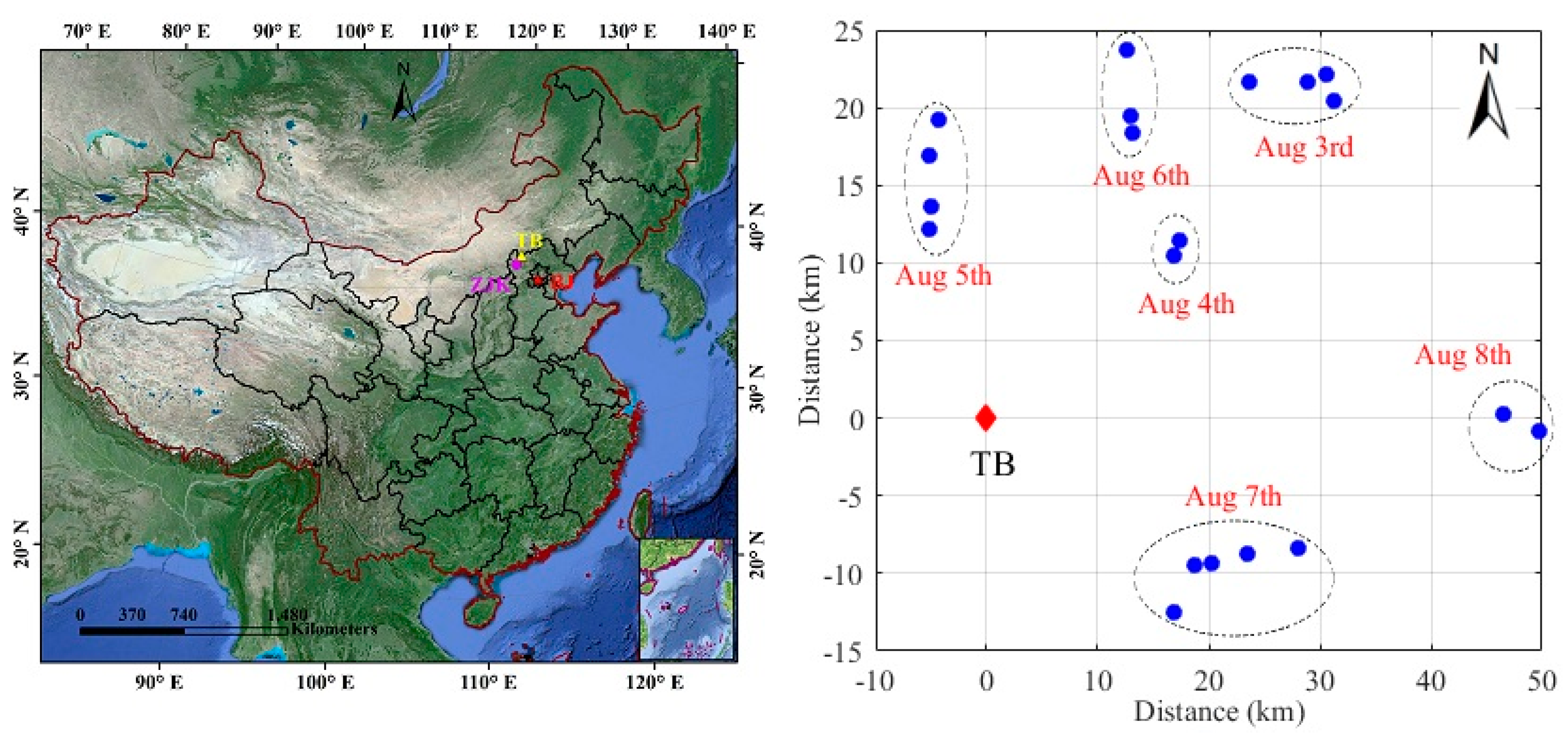
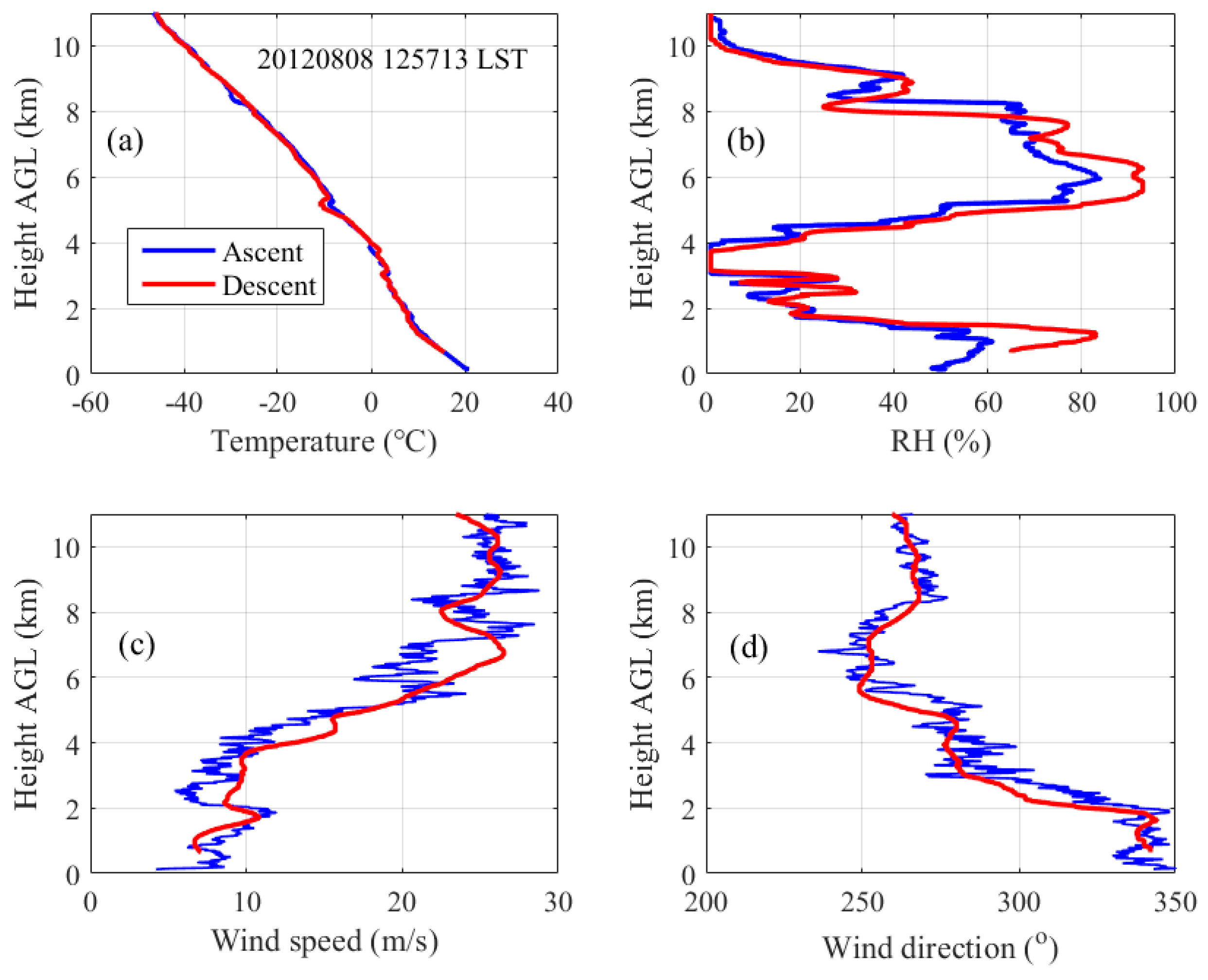
3.1. Site

The radiosonde campaign was performed at Taibus Banner (TB; 41.69° N, 115.23° E, 1380 m ASL; as shown in Figure 2), Inner Mongolia, China. TB is a typical grassland area located in the southwest of the Xilin Gol Prairie. It has a temperate continental arid climate with low annual precipitation (<400 mm) that intensively occurs in the summer months. The station is located approximately 300 km northwest of Beijing.

3.2. Data

The descending radiosonde data used by this study were collected at TB from 3 to 8 August 2012. The radiosondes were launched two to five times per day, resulting in a total of 20 profiles. Figure 2 shows the drift distances from the launching spot to when the radiosonde lost a signal during its descent period. They were mostly less than 50 km and were very close to the radiosondes released on the same day.

The maximum heights of the radiosonde exceed 10 km, after which it begins to descend. The minimum descent altitude with a radiosonde signal is generally ~0.5 km above the ground level (AGL). The radiosonde descent speed ranges from ~25 m/s at 10 km to ~15 m/s at 0.5 km AGL. It takes some extra time to reach the quasi-equilibrium state when the radiosonde begins to descend. The high descent speed at the high altitude of the troposphere may induce a large uncertainty in the VV retrievals since their magnitudes are usually dozens of centimeters per second or less. The radiosonde we used tends to provide a more stable performance at the low and middle troposphere [35]. Hence, only VVs at low and middle tropospheres (i.e., from 0.5 to 7 km AGL) are used in this study.

The radiosonde measures the atmospheric temperature, RH, horizontal wind speed and direction at a temporal resolution of 1 s during its ascent and descent periods. The response time of the temperature and humidity sensors is 0.8 and 1.5 s respectively. As an example, Figure 3 shows the measurement profiles from our last radiosonde launch at 12:57 local standard time (LST), 8 August 2012 when largest drift occurred. The temperature profiles during the ascent and descent periods were in a reasonable agreement. The RH profile observed during the descent was wetter than that during the ascent, which is likely due to a larger spatial variation in the water vapor during the drift of the radiosonde. Compared to the ascent, the horizontal wind speed and direction tended to be smoother during the descent period, which was also likely associated with the spatial variation and due in part to the coarse vertical resolution (a larger descent speed of the radiosonde).

To aid in the investigation of the VV retrieval, the ERA5 data were used to provide information pertaining to the large-scale synoptic circulation, surface atmospheric instability, and vertical velocity. ERA5 is the latest global atmospheric reanalysis dataset available from the European Centre for Medium-Range Weather Forecasts. The gridded data provides hourly estimates of a large number of atmospheric, land and oceanic climate variables. The data cover the Earth on a 30 km grid and resolve the atmosphere using 137 levels from the surface up to a height of 80 km. ERA5 includes information about uncertainties for all variables at reduced spatial and temporal resolutions. The pressure, temperature, zonal and meridional components of the wind, the convective available potential energy (CAPE), and the vertical velocity data over Inner Mongolia, were used. Additionally, a Weather Surveillance Radar-1998 Doppler (WSR-98D) radar deployed at Zhangjiakou (ZJK; 41.16° N, 114.69° E, 1425 m ASL; as shown in Figure 2). The radar base reflectively product was used to provide the temporal evolution of a convective cloud process over the TB site. The WSR-98D radar at ZJK is a C-band radar with a maximum range of 400 km [36]. The distance from this radar to the TB site is approximately 96 km.

3.3. Methodology

3.3.1. VV Estimation Algorithm

Following [30], we obtained the VV from the difference between the calculated radiosonde descent speed in still air (W_C in m/s) and the observed radiosonde descent speed (W_O in m/s): VV = W_C − W_O. A positive/negative value of the VV implies upward/downward air motion, respectively.

W_C can be calculated by using the following formula, based on the balance between gravity and the drag forces [29]:

$$M\times g=A\times \rho \times C\times W_C{}^2/2$$

(1)

where $M$ is the total mass of the radiosonde (~0.24 kg), hard ball (~0.32 kg) and string (~0.13 kg), which is weighed and recorded for each package set. $g$ is the acceleration due to gravity at the surface of Earth (in m s⁻²). $\rho$ is the vertical dry air density profile (in kg/m³), which can be calculated from the individual vertical profiles of the temperature and pressure. $A$ is the cross-sectional area of the hard ball (in m²), which is the same for every hard ball due to its constant diameter (i.e., 50 cm). This favors more accurate estimations of the vertical air motion compared to the soft parachute used by [30] because of the deformation and swing of the soft parachute. $C$ is the drag coefficient which varies with the altitude in this study; it was set as a constant parameter for the dropsonde in [30].

3.3.2. Radiosonde-Based Cloud Layer Identification

To aid the comprehension of the VV characteristics, a radiosonde-based cloud layer identification method developed by [37] was used. A brief description of the algorithm is presented here, while detailed procedures can be found in the above literature. The algorithm employs three height-resolving RH thresholds to determine the cloud layers, i.e., the minimum and maximum RH thresholds in cloud layers, and the minimum RH threshold within the distance of the two neighboring cloud layers. The RH is transformed with respect to ice for levels with a temperature below 0 ℃. This method was developed based on the Vaisala RS92 radiosonde, which had a higher RH detecting accuracy compared to other types of radiosondes [38]. The RH thresholds used to determine the cloud location by various radiosondes should be modified according to their different RH detecting accuracies [39]. The average dry bias of our radiosonde was about on the order of 10% from the surface to the middle troposphere [40]. Therefore, the above three RH thresholds for our radiosonde are 10% RH less than the values used for the Vaisala RS92 in [37].

4. Uncertainty Analysis and Credibility Assessment of VV Retrievals

Validating the VV has long been a daunting task, not only because of the lack of independent “truth” in VV measurements but also because of the inherently large variability of VV [26,30]. Both apply to this study. Here, we assess the credibility of the estimated VV by (1) an uncertainty analysis, and (2) examining the consistency of the retrieved VV with the radar- and radiosonde-observed cloud field and reanalysis data. The latter is achieved by conducting a composite analysis and a set of case studies.

Before proceeding, we first revisit some background knowledge of VV in order to aid in the interpretation of the credibility assessment. The VV of any air parcel has two components: VV_mean and VV’, in which VV_mean is the vertical velocity of the large-scale mean flow that is typically small in magnitude (several tens of cm s⁻¹ in fair weather conditions), and VV’ is the turbulent component that is highly variable and can have large values in highly convective weather systems. VV_mean, as a background VV, is much less variable than the small-scale VV’.

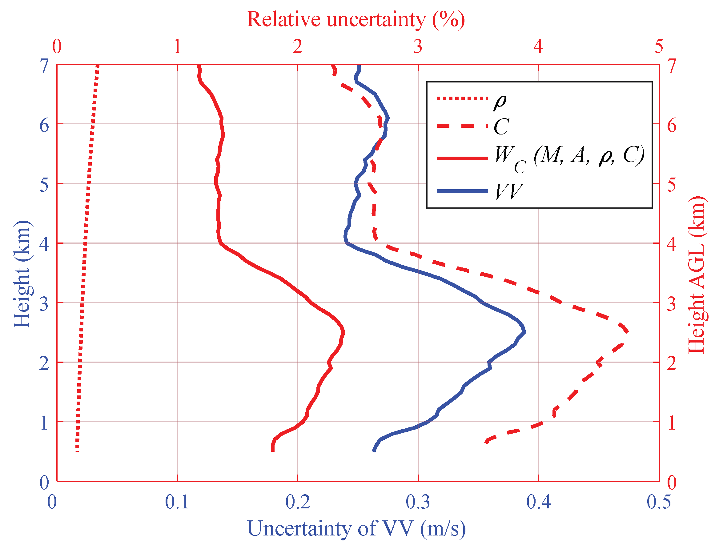
4.1. Uncertainty Estimation

According to the aforementioned VV estimation formula, its accuracy is determined by the uncertainties of W_O and W_C. The W_O is inferred from the Global Position System (GPS) data that is provided by the descending radiosonde. Although the absolute uncertainty of the GPS data can reach up to several or tens of meters, W_O is estimated from the relative position of the radiosonde. The uncertainty of W_O is less than 0.3 m/s [41]. To reduce the occasional noise and uncertainty, the vertical resolution of W_O was projected at a vertical resolution of 100 m for the radiosonde profile. Hence, the total uncertainty of W_O may be expected to be 0.3 m/s at most.

The calculation of $W_C$ is a function of $M$, $A$, $\rho$, and $C$:

$$W_C=W_C\left(M, A,\rho , C \right)$$

(2)

The uncertainty in W_C is a composite contribution from the individual uncertainties of these four different parameters. Their uncertainties are assumed to be random and follow Gaussian distributions; the Gaussian law of uncertainty propagation is thus applied to Equation (2). The overall relative uncertainty is defined as $\frac{\Delta W_C}{W_C}$ and is expressed as follows, with the results provided in

Table 1. Summary of the uncertainty existing in the descending radiosonde system.

	Magnitude	Absolute Uncertainty	Relative Uncertainty
$M$	690 g	1 g	0.14%
$A$	1964 cm2	7.8618 cm2	0.40%
$\rho$	0.4684–0.9665 kg/m3	0.0016 kg/m3	0.17–0.34%
$C$	0.3261–0.3319	0.0037–0.0078	2.29–4.74%
$W_C$	14.68–21.29 m/s	0.2393–0.3877 m/s	1.18–2.38%

:

$$\frac{\Delta W_C}{{\mathrm{W}}_{\mathrm{C}}}=\frac{1}{2}\sqrt{{(\frac{\Delta \mathrm{M}}{\mathrm{M}})}^2+{(\frac{\Delta \mathrm{A}}{\mathrm{A}})}^2+{(\frac{\Delta \mathsf{\rho }}{\mathsf{\rho }})}^2+{(\frac{\Delta \mathrm{C}}{\mathrm{C}})}^2}$$

(3)

$\Delta \mathrm{M}$ is assumed to be a constant value of 1 g, leading to a 0.14% relative uncertainty ($\frac{\Delta \mathrm{M}}{\mathrm{M}}$) after being divided by the typical total mass of the descending system at 690 g. The surface of the plastic foam ball is designed smoothly, expecting to remove or reduce the water accumulation on the ball during the flight. However, potential total mass increase might occur due to the effect of the rain or/and ice. This effect is ignored in the current study because its quantity is still unclear at present given the complexity of the moisture accumulation under different weather conditions. As the next step, it might be expected to address this issue through the combination of in-situ experimental measurements and model simulations. The diameter of the hard plastic foam ball is 50 cm, with an absolute uncertainty set at a constant value of 0.1 cm. This results in the relative uncertainty of $\frac{\Delta \mathrm{A}}{\mathrm{A}}$ being 0.40%.

In contrast with $M$ and $A$, the uncertainty contributions from $\rho$ and $C$ depend on the air pressure (or altitude) and temperature. Figure 4a presents the vertical distributions of the calculated $\rho$ for 20 radiosondes released over the TB site. Overall, small variabilities were found among different profiles; their mean values increased from ~0.47 kg/m³ at 7 km to 0.97 kg/m³ at 0.5 km. Vertical uncertainties of $\rho$ is mathematically derived from uncertainties of temperature (0.3 ℃) and pressure (1 hPa) data with the law of uncertainty propagation. As shown in Figure 5, the relative uncertainty is less than 1% for $\rho$ at all height levels.

$C$ depends on the Reynolds number (Re, being generally in the range of 3 × 10⁵). A transition often exists in Re from the boundary layer or turbulent layer to the free troposphere [33,42]. Additionally, other factors, such as free stream turbulence and unsteadiness of the ball during flight can also influence the value of $C$ [27]. Therefore, it is very difficult to estimate $C$ actually and it is challenging to use a uniform $C$ below a fixed altitude for the soundings. $C$ is set varied to find optimal values for the radiosonde whereas a constant $C$ is used for the dropsonde in [30]. Given the difficulties in estimating $C$ based on Re and the large uncertainty associated with other complex influence factors mentioned above, $C$ used in this study is derived as follows. Vertical descent speed profiles, which are almost smooth associated with the stable weather conditions according to the observation records, are selected. This leads to 6 almost smooth profiles selected from the 14 profiles collected under nonconvective conditions. A low-pass filter was then applied to these 6 profiles to remove the noise from the pendulum effect, self-induced ball motions, and other potential causes (such as turbulence). The filtered profiles data are deemed the radiosonde descent rate in still air, which are used to calculate vertical average $C$ and its standard deviation using the formula (1). The vertical $C$ varied little (between 0.32 and 0.33) at different height levels; its standard deviation tended to be larger below 4 km than that in the middle troposphere (Figure 4b). The mathematical estimation of uncertainty sources pertaining to $C$ is also very difficult due to the complex influence factors aforementioned. Therefore, the $C$ uncertainty from its vertical variability (i.e., standard deviation in Figure 4b) is analyzed in this study. As shown in Figure 5, a greater relative uncertainty, at most up to 4.74% at ~2.5 km AGL, is revealed for $\frac{\Delta \mathrm{C}}{\mathrm{C}}$. The large magnitude of $\frac{\Delta \mathrm{C}}{\mathrm{C}}$ below 4 km is most likely a result of the turbulence that occurs at the low troposphere [29,30].

The resultant relative and absolute uncertainties of W_C caused by the above four parameters are also shown in Figure 5. The maximum relative uncertainty ($\frac{\Delta W_C}{{\mathrm{W}}_{\mathrm{C}}}$) is 2.38%, which is mainly attributed to the large uncertainty of $C$. The absolute uncertainty of W_C is calculated by the relative uncertainty multiplied by the mean W_C (as presented in the following section), leading to the uncertainties varying between 0.24 and 0.39 m/s.

The resultant absolute uncertainty of the VV retrievals, obtained by the sum of both W_O and W_C, is estimated on the order of 0.54–0.69 m/s. Based on this, the descending radiosonde estimated VV may have the potential to capture and describe events with vertical air motions >0.69 m/s.

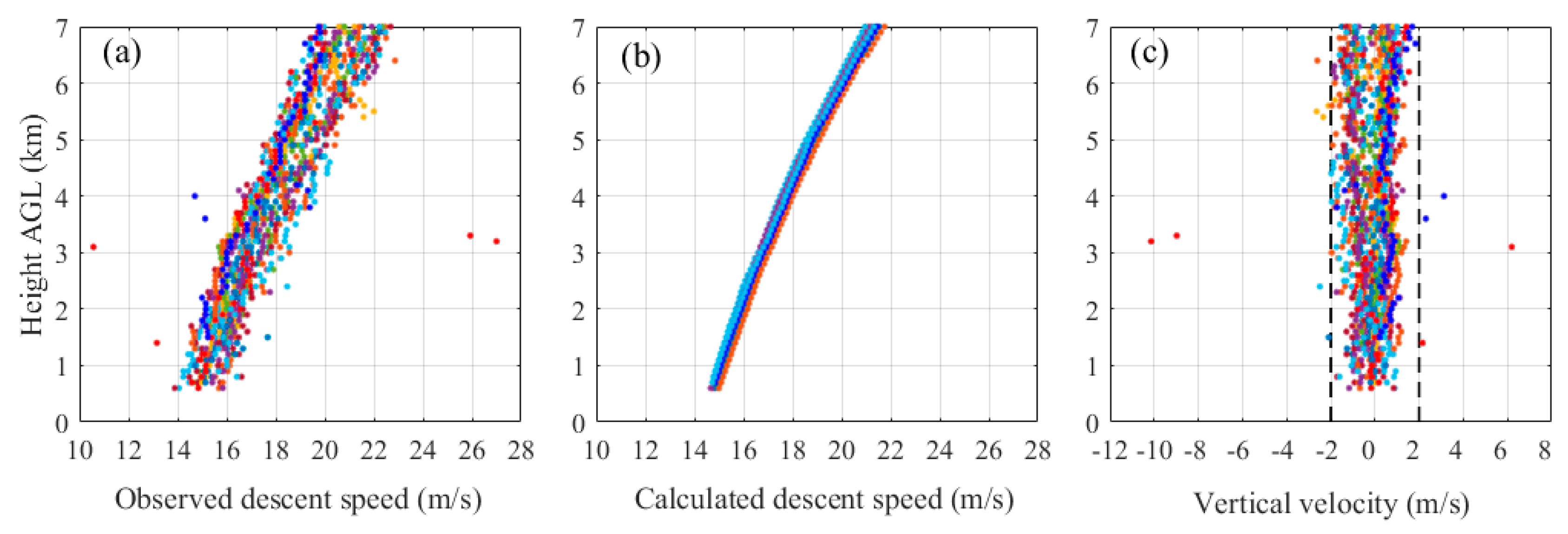
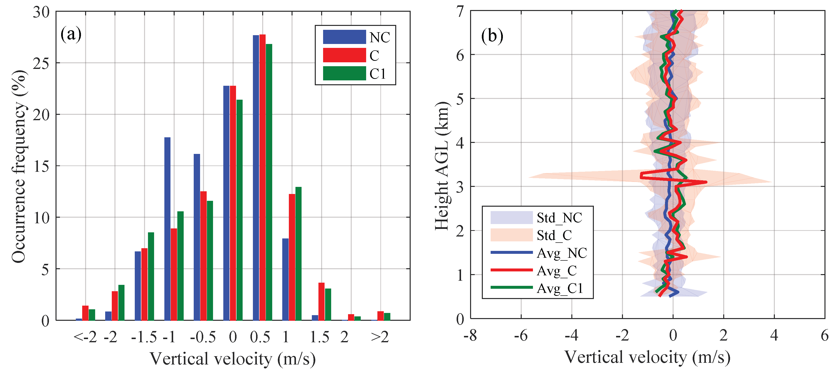
4.2. Composite Analysis

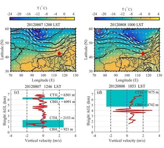
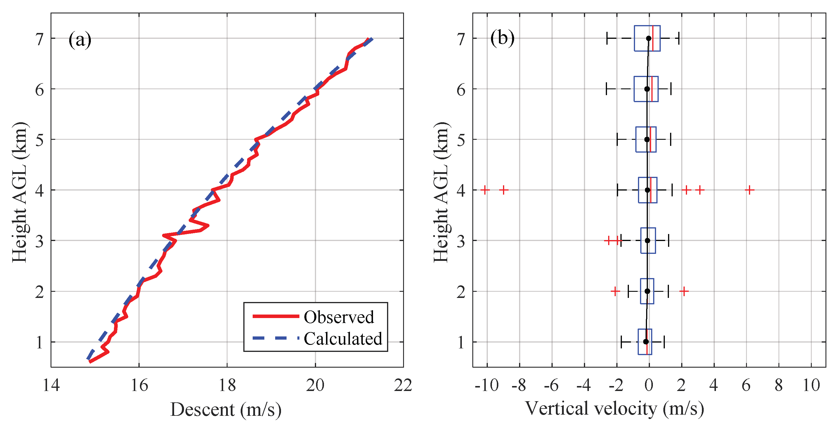
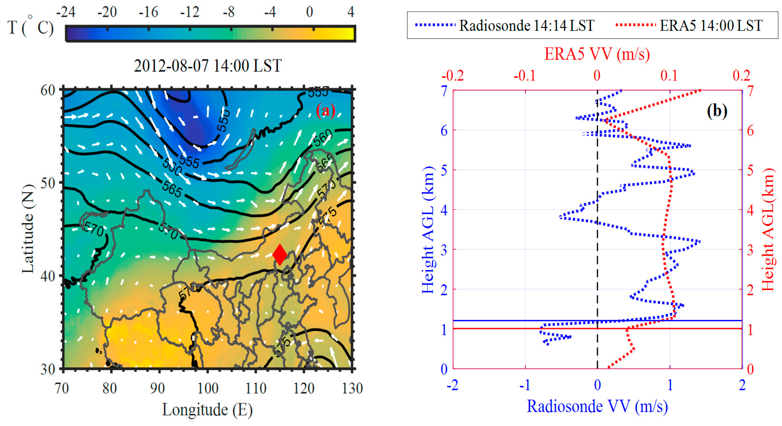
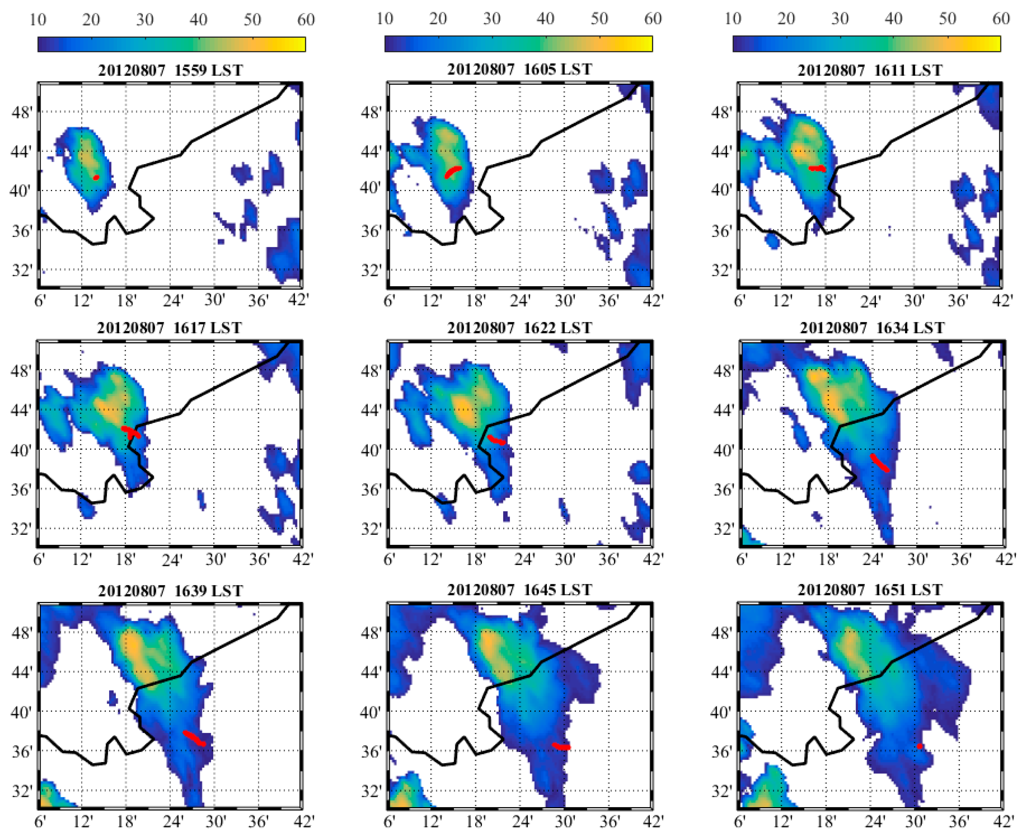
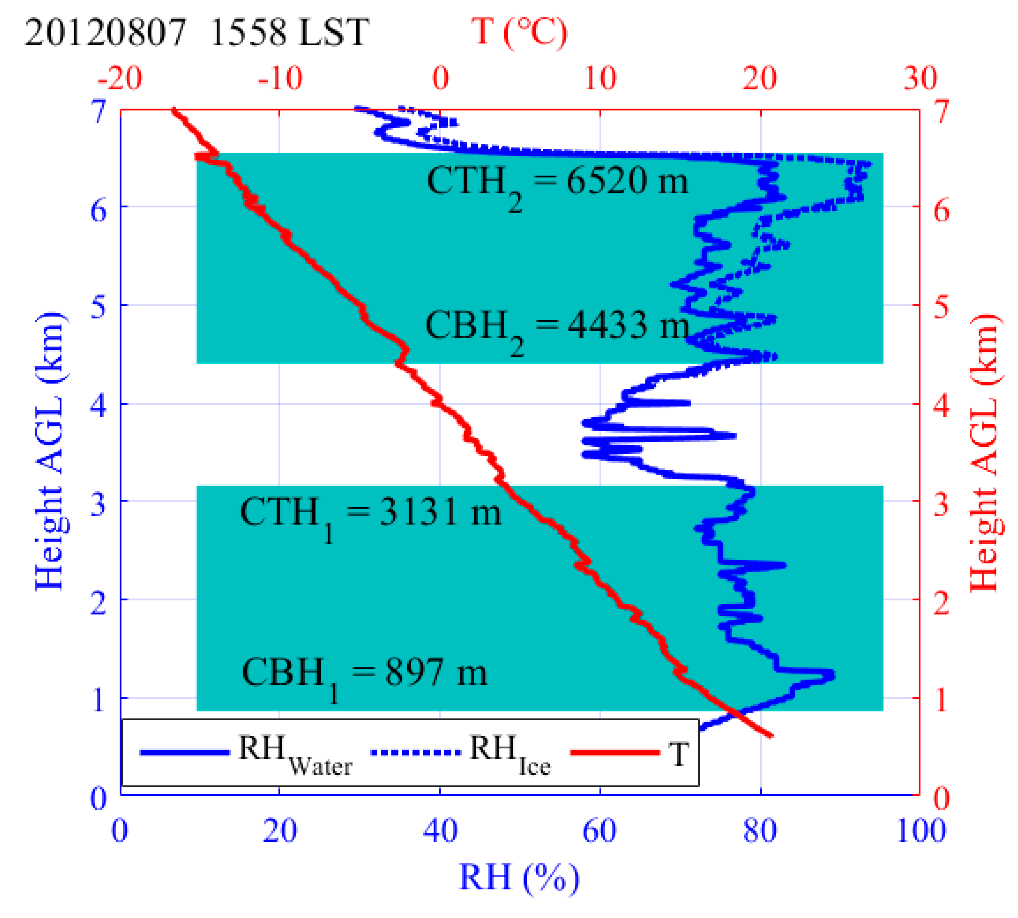
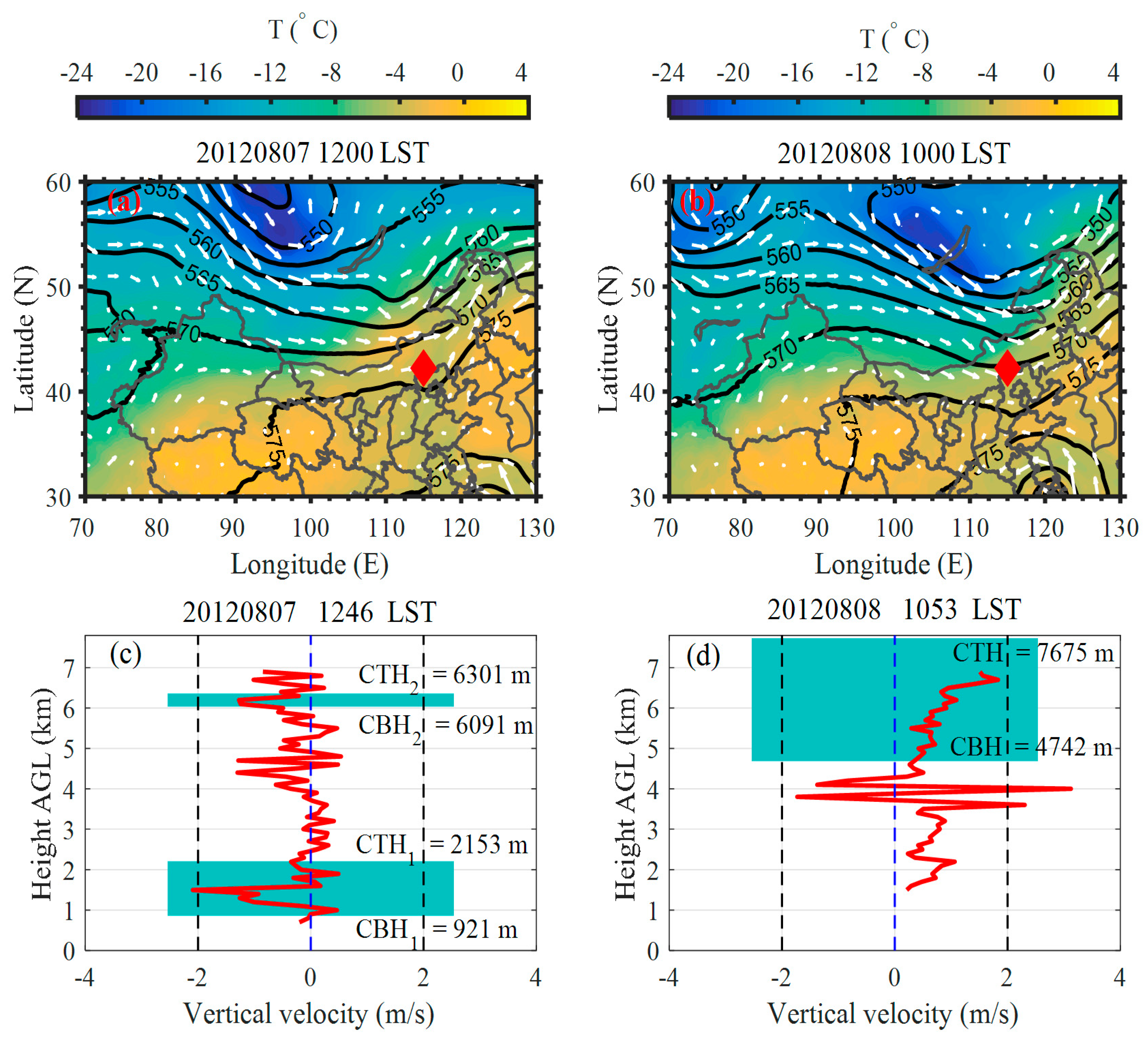
The mass and vertical air density derived from the individual radiosonde and the vertical mean drag coefficients are input into Equation (1) to calculate W_C in still air for each sounding. Figure 6 shows the vertical distributions of the observed and calculated radiosonde descent speed and the VV retrievals at a vertical resolution of 100 m from 20 radiosondes. In general, the observed radiosonde descent speed varied from ~20 m/s at 7 km to ~15 m/s in the boundary layer (Figure 6a). However, a closer view of the individual descent profiles revealed discrepancies in the magnitude of the descent speed among different profiles. Compared to the measurements, the calculated descents were smoother and presented better consistency among the different profiles (Figure 6b). The vast majority of VVs ranged from −1 m/s to 1 m/s, accounting for 80.2% of the data points (Figure 6c). It should also be noted that strong vertical air motions were occasionally detected by a few of the radiosonde profiles. For example, updrafts >2 m/s were detected by two radiosondes at the low and middle troposphere. In addition, violent updrafts with a VV >6 m/s and downdrafts with a VV <−10 m/s were observed by one radiosonde released at 15:58 LST 7 August 2012 (hereafter this extreme radiosonde case is referred to as RC_7th). Further investigations on these particular cases are presented in the following section.

The average vertical profiles of the radiosonde descent speed and VV from 20 radiosondes are displayed in Figure 7. The descent speeds from the measurements and calculations were generally close at most altitudes (Figure 7a). A relatively larger difference could be found at ~3 km between the two descent datasets at a more detailed level, which was manifested in the extreme outliers in Figure 7b. The medians and means of the VV were generally distributed at approximately 0 m/s at all height levels (Figure 7b).

The VV retrievals from the 20 radiosonde profiles were further divided into two categories: nonconvective (14 profiles) and convective (6 profiles) conditions, which are classified mainly according to the observation records, CAPE, and radar reflectivity. The nonconvective conditions are related to a clear sky or cloudy sky without precipitation and with a small CAPE (<150 J/kg) and reflectivity (<20 dBZ). The convective conditions are associated with a cloudy sky and precipitation (or thunderbolt) occurring [43,44]. Figure 8a shows the histogram distribution of the VV retrievals. A close occurrence frequency was exhibited by the two weather conditions for a VV between 0 and 0.5 m/s. However, compared to the nonconvective condition, the VV distribution was wider and skewed to the large values under the convective condition. In view of a certain bin for a VV >1 m/s, the occurrence frequency was always larger under convective conditions rather than that under nonconvective conditions, implying that there was a stronger updraft in the former weather condition. The occurrence frequency from the convective condition with the exception of the particular radiosonde case (RC_7th) is also shown in Figure 8a. A similar variation pattern was exhibited between all convective conditions and those with RC_7th discarded, indicating that the extreme RC_7th had little impact on the statistics of the VV distribution under convective conditions. The vertical averages of the VV and their standard deviations are presented in Figure 8b. The vertical VV was almost close to 0 m/s at all altitude levels under nonconvective conditions. In contrast, greater VV variations were exhibited under convective conditions. The incompleteness of the data below 1 km hindered us from analyzing the VV characters near the surface. An apparent difference was found by the two weather categories for a VV from 1 to 5 km, with stronger vertical air motion exhibited under convective activities. Dramatic deep convective systems, which could extend to the upper troposphere, did not occur during our experimental period, resulting in a small VV magnitude above 5 km under both convective and nonconvective conditions. The VV under all convective conditions and those with RC_7th discarded mostly agree well, except for at approximately 3 km.

4.3. Case Study

The VV measurements with absolute values of >10 m/s were detected by the RC_7th release. This section focuses on the details of this case and briefly introduces the other two cases with relatively large VV values.

According to the observation records, the cloud fraction increased from 90% at 09:00 LST to 100% at 15:00 LST 7 August over the TB site. The cumulus congestus transformed into cumulonimbus, which was accompanied by rain and lightning at 16:05 LST 7 August. As shown in Figure 9a (the synoptic system from ERA5 at 14:00 LST 7 August), the TB site was located at the trough of low pressure at 500 hPa, indicating upward motions of air according to omega equations [9]. In addition, the ERA5-based CAPE was 45.7 J kg⁻¹ at 14:00 LST, which jumped to 609.1 J kg⁻¹ when the rain started. Figure 9b shows the vertical air motions from the ERA5 data at 14:00 LST 7 August. A radiosonde was launched at 14:14 LST, which temporally matched the ERA5 data. The VV obtained by this radiosonde profile is also presented in Figure 9b for comparison. The ERA5 data indicated upward air motion during all altitude levels. The radiosonde showed downward motion near 3 km, straddling between two upward-motion layers with one in the lower atmosphere and one in the middle atmosphere. Compared to the radiosonde derived column-integrated VV (0.44 m/s), a smaller magnitude (0.07 m/s) and a less-structured VV were revealed by the ERA5. However, this difference is understandable by taking into account the followed factors. The ERA5 is a gridded data product which represents the average state of the vertical air motion within a certain spatial region. Several cm s⁻¹ is a typical value for large-scale vertical air motion. However, local deep convection may cause much larger VV values, which can be well expressed by the real-time and in situ measurement from the radiosonde along its descending path. Note that ERA5 dataset is only used to provide a qualitative comparison with the radiosonde measurements in this study; caution should be taken to the ERA5 VV value presented here since ERA5 do not explicitly resolve convection.

The reanalysis and the radiosonde-measured VV diverged dramatically in the boundary layers marked by the horizontal lines (Figure 9b). The reanalysis showed upward motions that were coherent with the free-tropospheric measurements, whereas the radiosonde showed a sudden shift to downward motions below the boundary layer. This is because the reanalysis VV data represent VV_mean and cannot resolve the turbulent component—VV’. In a planetary boundary layer that is highly turbulent, the rapidly varying VV’ should dominate the VV. This is well captured by the radiosonde data, which show negative VV values even though the cloud observations and synoptic conditions indicate upward air motions.

Figure 10 shows the temporal evolution of base reflectivity from the nearest C-band radar at ZJK from TB site (96 km) during the entire measurement period of the extreme radiosonde case –RC_7th. The color bar represents the radar reflectivity, with the red curve denoting the radiosonde drift path during the interval of each radar panel. The maximum reflectivity was ~60 dBZ for this case. The radiosonde gradually drifted from the core region to the borderland of this cloud system. As seen by both the experimental log and the radar echo, it was a significant convective cloud process.

The ground-based radar can provide the convection development process for this case (Figure 10). However, due to the long distance from the radar to the TB site causing very few data points to be generated in the vertical direction, it is not feasible for this radar to provide the vertical profile of this convective system along the radiosonde path. The radiosonde-based cloud retrieval algorithm is thus used to determine the vertical distribution of the cloud layer, as shown in Figure 11. One low cloud and one middle cloud were detected, with thicknesses of 2234 m and 2087 m, respectively. The tops of both cloud layers were capped by inversion layers. Figure 12a shows the observed vertical descent speed (blue line) and the radiosonde descent height as a function of the descending time (red line). The variation tendency of the temporal descent height was generally smooth during the whole altitude range, except for a sudden jump occurring at approximately 3 km that was reflected by a dramatic fluctuation in the observed descent speed profile. The VV profile superimposed on the cloud layers is shown in Figure 12b. Strong positive and negative VV occurred near the lower-level cloud top and even <−10 m above the cloud top, respectively. The switch between the updraft and the downdraft should be associated with the turbulence dissipation [14]. This was likely a typical case for convective clouds, characterized by strong moist updrafts in the cloud core surrounded by strong dry downdrafts to maintain the mass balance in the boundary layer. Yang [45] showed that different magnitudes of VV on the cloud top correspond to different stages of clouds (developing, mature, and dissipating stages). The large magnitude of the absolute VV at ~3 km should correspond to the vigorous developing stage of this convection cloud. In addition to the strong VV at the cloud top height, an evident updraft >2 m/s was ever presented at 1.4 km, which was close to the bottom of the cloud.

Figure 13 shows the other two radiosonde cases that detected relatively larger absolute VV (>2 m/s) compared to the general VV value. The two radiosondes were launched at 12:46 LST 7 August and 10:53 LST 8 August 2012, respectively. Their synoptic systems were similar to the previous case, i.e., the TB site was located in the low pressure at a 500 hPa level. Great VV variations were presented by both cases. The first case was a two-layered cloud configuration. A large VV was observed within the low-level cloud, with the strongest downdraft being −2.1 m/s at 1.5 km, located at the middle of this cloud layer. The VV then fluctuated between 4 and 5 km. The relatively larger absolute VV value of 1.3 m/s was retrieved at 6.2 km within the high-level cloud. Regarding the second case, one cloud layer with a thickness of 2.9 km was determined by the radiosonde. The VV was relatively stable below 3.5 km, followed by a noticeable variation of an updraft >3 m/s and a downdraft <−1 m/s that occurred within 1 km below the cloud base height. The VV measurements with the greatest values close to 2 m/s were also noted within the cloud layer.

5. Discussion and Conclusions

Vertical air motion has long been among the most difficult quantities to measure. Some progress has been made in air velocity retrieval in recent years by using ground-based and space-borne remote sensing instruments. However, such information is still insufficient for most parts of the world, including a large territory of China. Thus, more in situ observations are desperately needed. In this study, a descending radiosonde system is developed based on the conventional radiosonde operated at upper air observation stations.

By using descending radiosonde data collected at a local site in north China during the summer of 2012 (from 3 to 8 August), the vertical air velocity was derived at the low and middle troposphere. The VV generally varied from −1 m/s to 1 m/s, accounting for 80.2% of all analyzed data points. Compared to the nonconvective condition, the VV distribution was wider and skewed to the large value under the convective condition. Apparent vertical air motion was exhibited below 5 km under the convective activities. The average VV throughout the entire profiles was close to 0 m/s under noconvective conditions. Strong vertical air motion (>2 m/s) was observed by a few radiosonde profiles. Radiosonde-based VV profiles showed similar gross patterns with retrievals from the reanalysis data for a case analysis. Moreover, the detailed structure of the instant air motion in the vicinity of the cloud boundaries (i.e., top and base), with an absolute VV >10 m/s occurring in the convection weather system, was well captured by the in situ radiosonde observational technique.

The radiosonde has been in routine operation at more than 120 stations in China for over a decade. In view of the extra low-cost attached to the routine radiosonde operation, it is hoped that this system could be applied to this radiosonde network, and thus, provide additional VV information over a large space of China. This would be beneficial for monitoring climate change and may be used to validate and potentially improve the dynamic parameterization in model simulations.

The preliminary results in this study showed that the technique presented here could be used to derive vertical air motion, which is likely to be deployed for conventional operations and scientific applications. However, taking the following factors into account, only the VV at the low and middle troposphere are discussed in this study: (1) it will take some time for the radiosonde from dropping at a high troposphere to achieve posture balance, and thereby, the quasi-equilibrium state of descent, (2) the great radiosonde descent speed at the upper troposphere could induce large uncertainty in VV retrievals due to their small conventional magnitudes (usually less than dozens of centimeters), and (3) the radiosonde we used tends to provide a more stable performance at the low and middle troposphere. Future studies are needed to reduce the course of the posture balance and to decrease the radiosonde descent speed, thereby favoring a reasonable VV estimation at high altitude levels as well as a better VV retrieval at low/middle altitude levels. Radiosonde descent rate profiles under stable weather conditions are selected and processed to calculate $\mathrm{C}$ in this study. More attention should be paid to finding a better estimation method of $\mathrm{C}$ and its uncertainty, to improve the VV retrievals. Due in part to the generally small magnitude and high temporal and spatial variability of the vertical air, it is currently difficult to collocate objects detected by a drifting radiosonde and other measurements (e.g., fixed ground-based) to make a point-to-point data comparison. The uncertainty estimation of our system was deduced from the numerical calculation in this study. The results indicated that this method had the potential to capture and describe events with vertical air motions >0.69 m/s, which is useful for convective weather study, as shown by the case analysis with VV > 2m/s and even up to 10 m/s. Further studies will focus on the accurate validation of the method. Satellite measurements and/or a network composed of combined Doppler lidar/radar that can cover the predicted drifting path of the radiosonde should help achieve a careful assessment of the VV method, especially in case of large balloon drift and in cloudy conditions.

References

1. Heymsfield, A.J. Precipitation Development in Stratiform Ice Clouds: A Microphysical and Dynamical Study. J. Atmos. Sci. 1977, 34, 367–381. [Google Scholar] [CrossRef] [Green Version]
2. Li, Z.; Lau, W.K.M.; Ramanathan, V.; Wu, G.; Ding, Y.; Manoj, M.G.; Liu, J.; Zhou, T.; Fan, J.; Rosenfeld, D.; et al. Aerosol and monsoon climate interactions over Asia. Rev. Geophys. 2016, 54, 866–929. [Google Scholar] [CrossRef]
3. Zhao, B.; Jiang, J.H.; Diner, D.J.; Su, H.; Gu, Y.; Liou, K.N.; Jiang, Z.; Huang, L.; Takano, Y.; Fan, X.; et al. Intra-annual variations of regional aerosol optical depth, vertical distribution, and particle types from multiple satellite and ground-based observational datasets. Atmos. Chem. Phys. 2018, 18, 11247–11260. [Google Scholar] [CrossRef] [PubMed] [Green Version]
4. Paluch, I.R.; Lenschow, D.H. Stratiformcloud formation in the marine boundary layer. J. Atmos. Sci. 1991, 48, 2141–2158. [Google Scholar] [CrossRef]
5. Sun, J.; Leighton, H.; Yau, M.K.; Ariya, P. Numerical evidence for cloud droplet nucleation at the cloud-environment interface. Atmos. Chem. Phys. 2012, 12, 12155–12164. [Google Scholar] [CrossRef] [Green Version]
6. Leary, C.A.; Houze, R.A. The contribution of mesoscale motions to the mass and heat fluxes of an intense tropical convective system. J. Atmos. Sci. 1980, 37, 784–796. [Google Scholar] [CrossRef]
7. Stern, D.P.; Aberson, S.D. Extreme vertical winds measured by dropwindsondes in hurricanes. In Proceedings of the 27th Conference on Hurricanes and Tropical Meteorology, Monterey, CA, USA, 28 April 2006; Available online: http://ams.confex.com/ams/pdfpapers/108766.pdf (accessed on 8 May 2019).
8. Kim, Y.J.; Eckermann, S.D.; Chun, H.Y. An overview of the past, present and future of gravity-wave drag parameterization for numerical climate and weather prediction models. Atmos. Ocean 2003, 41, 65–98. [Google Scholar]
9. Holton, J.R. An Introduction to Dynamic Meteorology; Academic Press: San Diego, CA, USA, 1922; p. 507. [Google Scholar]
10. Lenschow, D.H.; Stephens, P.L. The role of thermals in the convective boundary layer. Bound. Layer Meteor. 1980, 19, 509–532. [Google Scholar] [CrossRef]
11. Greenhut, G.K.; Singh Khalsa, S.J. Updraft and downdraft events in the atmospheric boundary layer over the equatorial Pacific Ocean. J. Atmos. Sci. 1982, 39, 1803–1818. [Google Scholar] [CrossRef]
12. Saïd, F.; Canut, G.; Durand, P.; Lohou, F.; Lothon, M. Seasonal evolution of boundary-layer turbulence measured by aircraft during the AMMA 2006 Special Observation Period. Quart. J. R. Meteor. Soc. 2010, 136, 47–65. [Google Scholar] [CrossRef]
13. Balsley, B.B.; Ecklund, W.L.; Carter, D.A.; Riddle, A.C.; Gage, K.S. Average vertical motions in the tropical atmosphere observed by a radar wind profiler on Pohnpei (7oN latitude, 157oE longitude). J. Atmos. Sci. 1988, 45, 396–405. [Google Scholar] [CrossRef]
14. Shupe, M.D.; Kollias, P.; Poellot, M.; Eloranta, E. On deriving vertical air motions from cloud radar Doppler spectra. J. Atmos. Ocean. Technol. 2008, 25, 547–557. [Google Scholar] [CrossRef]
15. Kollias, P.; Albrecht, B.A.; Lhermitte, R.; Savtchenko, A. Radar observations of updrafts, downdrafts, and turbulence in fair-weather cumuli. J. Atmos. Sci. 2001, 58, 1750–1766. [Google Scholar] [CrossRef]
16. Ansmann, A.; Fruntke, J.; Engelmann, R. Updraft and downdraft characterization with Doppler lidar: Cloud-free versus cumuli-topped mixed layer. Atmos. Chem. Phys. 2010, 10, 7845–7858. [Google Scholar] [CrossRef]
17. Contini, D.; Mastrantonio, G.; Viola, A.; Argentini, S. Mean vertical motions in the PBL measured by Doppler sodar: Accuracy, ambiguities, and possible improvements. J. Atmos. Oceanic Technol. 2004, 21, 1532–1544. [Google Scholar] [CrossRef]
18. Zhao, K.; Wang, M.; Xue, M.; Fu, P.; Yang, Z.; Chen, X.; Zhang, Y.; Lee, W.; Zhang, F.; Lin, Q.; et al. Doppler radar analysis of a tornadic miniature supercell during the Landfall of Typhoon Mujigae (2015) in South China. Bull. Amer. Meteor. Soc. 2017, 98, 1821–1831. [Google Scholar] [CrossRef]
19. Zheng, Y.; Rosenfeld, D. Linear relation between convective cloud base height and updrafts and application to satellite retrievals. Geophys. Res. Lett. 2015, 42, 6485–6491. [Google Scholar] [CrossRef]
20. Zheng, Y.; Rosenfeld, D.; Li, Z. Satellite inference of thermals and cloud base updraft speeds based on retrieved surface and cloud base temperatures. J. Atmos. Sci. 2015, 72, 2411–2428. [Google Scholar] [CrossRef]
21. Zheng, Y.; Rosenfeld, D.; Li, Z. Quantifying cloud base updraft speeds of marine stratocumulus from cloud top radiative cooling. Geophys. Res. Lett. 2016, 43, 11407–11413. [Google Scholar] [CrossRef]
22. Luo, Z.J.; Jeyaratnam, J.; Iwasaki, S.; Takahashi, H.; Anderson, R. Convective vertical velocity and cloud internal vertical structure: An A-Train perspective. Geophys. Res. Lett. 2014, 41, 723–729. [Google Scholar] [CrossRef]
23. Treddenick, D.S. A comparison of aircraft and Jimsphere wind measurements. J. Appl. Meteor. 1971, 10, 309–312. [Google Scholar] [CrossRef]
24. Franklin, J.; Black, M.L.; Valde, K. GPS dropwindsonde wind profiles in hurricanes and their operational implications. Weather Forecast. 2003, 18, 32–44. [Google Scholar] [CrossRef]
25. Gallice, A.; Wienhold, F.G.; Hoyle, C.R.; Immler, F.; Peter, T. Modeling the ascent of sounding balloons: Derivation of the vertical air motion. Atmos. Meas. Tech. 2011, 4, 2235–2253. [Google Scholar] [CrossRef]
26. Bony, S.; Stevens, B. Measuring area-averaged vertical motions with dropsondes. J. Atmos. Sci. 2019, 76, 767–783. [Google Scholar] [CrossRef]
27. Lalas, D.P.; Einaudi, F. Tropospheric gravity waves: Their diction by and influence on rawinsonde balloon data. Quart. J. R. Meteor. Soc. 1980, 106, 855–864. [Google Scholar] [CrossRef]
28. McHugh, J.P.; Dors, I.; Jumper, G.Y.; Roadcap, J.R.; Murphy, E.A.; Hahn, D.C. Large variations in balloon ascent rate over Hawaii. J. Geophys. Res. 2008, 113, D15123. [Google Scholar] [CrossRef]
29. Johansson, C.; Bergström, H. An auxiliary tool to determine the height of the boundary layer. Bound. Layer Meteor. 2005, 115, 423–432. [Google Scholar] [CrossRef]
30. Wang, J.; Bian, J.; Brown, W.O.; Cole, H.; Grubišić, V.; Young, K. Vertical Air Motion from T-REX Radiosonde and Dropsonde Data. J. Atmos. Ocean. Technol. 2009, 26, 928–942. [Google Scholar] [CrossRef]
31. Wick, G.A.; Hock, T.F.; Neiman, P.J.; Vomel, H.; Black, M.L.; Spackman, J.R. The NCAR–NOAA Global Hawk Dropsonde System. J. Atmos. Ocean. Technol. 2018, 35, 1585–1604. [Google Scholar] [CrossRef]
32. Wu, C.C.; Chou, K.H.; Lin, P.H.; Aberson, S.D.; Peng, M.S.; Nakazawa, T. The impact of dropwindsonde data on typhoon track forecasts in DOTSTAR. Weather Forecast. 2007, 22, 1157–1176. [Google Scholar] [CrossRef]
33. MacCready, P.B. Comparison of some balloon techniques. J. Appl. Meteor. 1965, 4, 504–508. [Google Scholar] [CrossRef]
34. Nash, J.; Oakley, T.; Vömel, H.; Li, W. WMO Intercomparison of High Quality Radiosonde Systems, Yangjiang, China, 12 July–3 August 2010. Tech. Rep., WMO, 2011, WMO/TD-No. 1580, Instruments and Observing Methods Report No. 107. Available online: http://library.wmo.int/pmb_ged/wmo-td_1580.pdf (accessed on 10 December 2018).
35. Xie, Q.; Huang, K.; Wang, D.; Yang, L.; Chen, J.; Wu, Z.; Li, D.; Liang, Z. Intercomparison of GPS radiosonde soundings during the eastern tropical Indian Ocean experiment. Acta Oceanol. Sin. 2014, 33, 127–134. [Google Scholar] [CrossRef]
36. Hou, T.; Lei, H.; Yang, J.; Hu, Z.; Feng, Q. Investigation of riming within mixed-phase stratiform clouds using Weather Research and Forecasting (WRF) model. Atmos. Res. 2016, 178–179, 291–303. [Google Scholar] [CrossRef]
37. Zhang, J.; Li, Z.; Chen, H.; Cribb, M. Validation of a radiosonde-based cloud layer detection method against a ground-based remote sensing method at multiple ARM sites. J. Geophys. Res. 2013, 118, 846–858. [Google Scholar] [CrossRef] [Green Version]
38. Miloshevich, L.M.; Vömel, H.; Whiteman, D.N.; Lesht, B.M.; Schmidlin, F.J.; Russo, F. Absolute accuracy of water vapor measurements from six operational radiosonde types launched during AWEX-G and implications for AIRS validation. J. Geophys. Res. 2006, 111, D09S10. [Google Scholar] [CrossRef]
39. Zhang, J.; Chen, H.; Bian, J.; Xuan, Y.; Duan, Y.; Cribb, M. Development of cloud detection methods using CFH, GTS1, and RS80 radiosondes. Adv. Atmos. Sci. 2012, 29, 236–248. [Google Scholar] [CrossRef]
40. Bian, J.; Chen, H.; Vömel, H.; Duan, Y.; Xuan, Y.; Lü, D. Intercomparison of humidity and temperature sensors: GTS1, Vaisala RS80, and CFH. Adv. Atmos. Sci. 2011, 28, 139–146. [Google Scholar] [CrossRef]
41. Guo, Q.Y.; Li, F.; Guo, K.; Yang, R.K. Comparative analysis of new GPS and GTS1-2 radiosondes. Meteor. Sci. Technol. 2005, 43, 59–64, (In Chinese with English Abstract). [Google Scholar]
42. Vennard, J.K. Elementary Fluid Mechanics, 7th ed.; John Wiley & Sons: Hoboken, NJ, USA, 1955; p. 401. [Google Scholar]
43. Shi, H.; Chen, H.; Xia, X.; Fan, X.; Zhang, J.; Li, J.; Ling, C. Intensive radiosonde measurements of summertime convection over the Inner Mongolia grassland in 2014: Difference between shallow cumulus and other conditions. Adv. Atmos. Sci. 2017, 34, 783–790. [Google Scholar] [CrossRef]
44. Zhuang, Y.; Fu, R.; Marengo, J.A.; Wang, H. Seasonal variation of shallow-to-deep convection transition and its link to the environmental conditions over the Central Amazon. J. Geophys. Res. 2017, 122, 2649–2666. [Google Scholar] [CrossRef]
45. Yang, J.; Wang, Z.; Heymsfield, A.J.; French, J.R. Characteristics of vertical air motion in isolated convective clouds. Atmos. Chem. Phys. 2016, 16, 10159–10173. [Google Scholar] [CrossRef] [Green Version]
Figure 1. Schematic (not to scale) of the radiosonde payload for launch. A hard plastic foam ball with a diameter of 50 cm acted as the parachute. T and C denote the timer and cutter.
Remotesensing 11 01538 g001
Figure 2. Left panel: The campaign site at Taibus Banner (TB; yellow triangle) which is located approximately 300 km northwest of Beijing (BJ; red star), and the deployment of a C-band radar at Zhangjiakou (ZJK; pink dots). Right panel: drift distance (blue dots) of 20 radiosondes from the launch site when the detecting signal was lost during their descent periods; the red triangle denotes the launch site at TB; radiosondes released on the same day are encircled by a dashed line.
Remotesensing 11 01538 g002
Figure 3. Profiles of (a) temperature, (b) RH, (c) horizontal wind speed and (d) horizontal wind direction provided by the radiosonde launched at 12:57 LST August 8, 2012, over the TB site. The blue and red lines represent the measurements collected during the ascent and descent periods, respectively.
Remotesensing 11 01538 g003
Figure 4. The vertical profiles of (a) the air density and (b) the average drag coefficient (red line) over the TB site. The shaded green areas in panel (b) represent the standard deviation of the drag coefficient.
Remotesensing 11 01538 g004
Figure 5. Relative uncertainty of ρ (short dashed red line), C (long dashed red line), the resultant relative uncertainties of WC (solid red line) caused by the four parameters (i.e., M ,   A ,   ρ , and C ) and the induced resultant uncertainty of the VV (solid blue line).
Remotesensing 11 01538 g005
Figure 6. Vertical distributions of (a) the observed descent speed, (b) the calculated descent speed, and (c) the vertical velocity of air from 20 radiosondes (represented by different colors).
Remotesensing 11 01538 g006
Figure 7. (a) Vertical average of 20 radiosonde profiles of the observed descent speed (red line) and the calculated descent speed (blue lines); (b) Box-and-whisker plots of the vertical velocity spaced at 1 km intervals from 20 radiosonde profiles, including the median (red line in the box), 25th and 75th percentiles (ends of the box), 5th and 95th percentiles (ends of the whiskers), and means (black dots).
Remotesensing 11 01538 g007
Figure 8. (a) Histogram distribution of the radiosonde-based vertical velocity under nonconvective conditions (NC; blue bar), all convective conditions (C; red bar), and convective conditions with the exception of the extreme radiosonde case –RC7th (C1; green bar). (b) Vertical averages of the vertical velocity under nonconvective conditions (Avg_NC; blue line), all convective conditions (Avg_C; red line), and convective conditions with the exception of RC7th (Avg_C1; green line). Shaded regions represent the standard deviation under nonconvective (Std_NC) and all convective conditions (Std_C).
Remotesensing 11 01538 g008
Figure 9. (a) Synoptic system analysis over the TB site from the ERA5 data at 500 hPa at 14:00 LST on 7 August 2012. The white arrow is the wind speed and direction; the maximum value of the winds is 26 m s−1; the black lines are the geopotential height (units: gpm); the color shading represents the temperature (units: °C); and the red diamond is the location of TB site. (b) Vertical velocity (VV) of air from radiosonde released at 14:14 LST (dashed blue lines) and the ERA5 analysis data at 14:00 LST (dashed red lines) on 7 August 2012. The VV values of 0 m/s are denoted by the dashed black line. The solid blue line is a boundary layer height (BLH) retrieved from the radiosonde data (1210 m) and the solid red line is the BLH from the ERA5 data (1010 m).
Remotesensing 11 01538 g009
Figure 10. The temporal evolution of reflectivity from the C-band radar at ZJK during the measurement period of the radiosonde launched at 15:58 LST 7 August 2012, over the TB site. The latitude and longitude integers are 41° N and 115° E, respectively; only their minutes are labeled. The color bar represents the radar reflectivity (dBZ); the red curve denotes the radiosonde drift path during the interval of each radar panel; and the black line illustrates the geographic boundaries.
Remotesensing 11 01538 g010
Figure 11. Cloud layers retrieved from the radiosonde launched at 15:58 LST 7 August 2012 (RC7th) over the TB site. Cyan shading marks the extent of the cloud layer. The cloud base heights (CBH1 for the lower layer and CBH2 for the upper layer) and their corresponding cloud top heights (CTH1 and CTH2) of the two cloud layers are noted. The radiosonde vertical profiles of RH with respect to water, RH with respect to ice when the temperatures are less than 0 °C, and the temperature are shown by the solid blue line, the dashed blue line, and the solid red line, respectively.
Remotesensing 11 01538 g011
Figure 12. (a) Observed descent speed (dashed blue line) and the descending height as a function of time (solid red line) for the radiosonde launched at 15:58 LST 7 August 2012 (RC7th). (b) The vertical velocity of air (red line) superimposed on the cloud layers (cyan shadings) with the base heights (CBH1 and CBH2) and top heights (CTH1 and CTH2) noted. The vertical velocity values of −2 m/s, 0 m/s and 2 m/s are denoted by the dashed lines colored black, blue and black, respectively.
Remotesensing 11 01538 g012
Figure 13. Panels (a,b) show the synoptic system analysis, which is the same as Figure 9b but at 12:00 LST on 7 August and 10:00 LST on 8 August 2012, respectively. Panels (c,d) denote the vertical velocity, which are the same as in Figure 12b but for the other two radiosondes launched at 12:46 LST 7 August and 10:53 8 August 2012, respectively.
Remotesensing 11 01538 g013