Derivation of Vegetation Optical Depth and Water Content in the Source Region of the Yellow River using the FY-3B Microwave Data

Abstract

This study uses the brightness temperature at the given microwave frequency (18.7 GHz) from the Microwave Radiation Imager (MWRI) on-board the Fengyun-3B (FY-3B) satellite to improve the τ-ω model by considering the radiative contribution from waterbody in the pixels over the wetland of the Yellow River source region, China. In order to retrieve vegetation optical depth (VOD), a dual-polarization slope parameter is defined to express the surface emissivity in the τ-ω model as the sum of soil emissivity and waterbody emissivity. In the regions with no waterbody, the original τ-ω model without considering waterbody impact is used to derive VOD. With use of the field observed vegetation water content (VWC) in the source region of the Yellow River during the summer of 2012, a regression relationship between VOD and VWC is established and then the vegetation parameter b is estimated. The relationship is employed to derive the spatial VWC during the entire vegetation growing period. The VOD retrieved is invalid and failed in some part of the study area by using the previous τ-ω model, while the results from the improved τ-ω model indicate that the VOD is in the range of 0.20 to 1.20 and the VWC is in the range of 0.20kg/m² to 1.40kg/m² in the entire source region of the Yellow River in 2012. Both VOD and VWC exhibit a pattern of low values in the west part and high values in the east part. The largest regional variations appear along the Yellow River. The comparison between the remote-sensing-estimated VWC and the ground-measured VWC gives the root mean square error of 0.12kg/m². These assessments reveal that with considering the fractional seasonal wetlands in the source region of the Yellow River, the microwave remote sensing measurements from the FY-3B MWRI can be successfully used to retrieve the VWC in the source region of the Yellow River.

1. Introduction

Vegetation water content, vegetation canopy biomass, and soil moisture strongly affect fluxes of the surface water vapor and energy, control the proportion of surface sensible heat, and latent heat allocated to the usable surface energy, as well as the proportion of rainfall among the surface runoff, infiltration, and evapotranspiration, and thus can have significant impacts on numerical weather, climate and hydrologic predictions [1,2]. Optical-infrared satellite remote sensing, such as the Normalized Difference Vegetation Index (NDVI) and Leaf-Area Index (LAI), is commonly used to determine vegetation water content. However, clouds, aerosols, and solar illumination effects degrade the ability to monitor vegetation information. Satellite microwave observations are insensitive to clouds at lower frequencies and independent of solar illumination [3]. Currently, soil moisture retrievals using microwave radiometers have a high accuracy over bare soil or sparse vegetation coverage area, whereas ongoing challenges remain in high vegetated regions, due to lack of knowledge about the properties of vegetation structure, vegetation optical depth (VOD), vegetation water content (VWC), and biomass of canopy [3,4,5]. To accurately retrieve soil moisture, passive soil moisture retrievals must properly account for the effect of VOD, so developing a feasible VOD algorithm is necessary for soil moisture retrievals.

The VOD is a variable that characterizes the contribution of vegetation canopy decay to soil radiation and increases with vegetation density. Most VOD retrievals are conducted simultaneously with soil moisture retrievals [6,7]. As a useful indicator for understanding vegetation state and variability, VOD has also been widely used in a proxy of biomass [8], phenology metrics like growing season length and start of season [9,10], forest and agriculture monitoring [11], land evaporation estimation [12], and vegetation water stress [13].

Many studies revealed that VOD is less prone to saturation effect than optical vegetation index which is sensitive to the green components [14]. Meesters et al. [15] proposed a nonlinear iterative algorithm, which can simultaneously derive both soil moisture and VOD. In order to minimize the atmosphere impacts and soil surface emission signals, Shi et al. [16,17] proposed the passive microwave vegetation indices (MVIs) index that depends only on vegetation properties such as vegetation fractional coverage, biomass, water content, temperature, and geometry of vegetation canopy. In the microwave bands (>5.0 GHz), the brightness temperatures are obviously affected by absorption and scattering of vegetation, whereas the L-band can almost penetrate most of the dense natural vegetation. However, VOD retrievals at L-band can increase potential sensitivity at higher biomass levels, and have severe radio frequency interference (RFI) contamination and are more sensitive to soil moisture at lower VOD levels [18]. High microwave frequencies (＞18.7 GHz), such as K-band, X-band, or C-band, have also been used in previous studies [8,19]. For higher frequencies ＞18.7 GHz, however, water vapor and cloud liquid water in various atmospheric layers absorb and emit scattered radiation [14]. Therefore, the 18.7 GHz frequency has low RFI and can reduce atmosphere and soil moisture sensitivities to other channels [6]. Jones et al. [14,19] retrieved VOD based on the τ-ω model from both the 18.7 GHz and 23 GHz channels (K-band and X-band frequencies), by determining the influence of open water fraction of each pixel and with given albedo. The VOD parameter contributes to a more comprehensive view of land surface phenology.

Vegetation water content (VWC) is another important parameter that affects microwave signals. Since the 1990s, several visible spectral indexes have been proposed to describe VWC, including normalized difference vegetation index(NDVI), water band index (WBI), normalized difference water index (NDWI), and moisture stress index (MSI) [20]. There are several factors that may contribute to limitation of the global VWC study. Products with spectral reflectance and index usually contain noise from the background (e.g., soil and exposed waterbodies). Measurements at the visible/near-infrared band mostly reflect greenness of vegetation because of the limitation of penetrating capacity, which directly affects accuracy of leaf water content estimation. Therefore, studies of the global VWC are limited [21,22,23,24,25]. Furthermore, the visible/near-infrared vegetation index reflects only vegetation information on the top of the canopy [26], so it cannot be applied for accurately monitoring VWC. Measurements using passive microwave radiometers are more sensitive to variations in the characteristics of vegetation canopy, and can be directly used to retrieve canopy VWC without affected by weather conditions. These observations have the potential to be used for all-weather monitoring of regional vegetation canopy. VWC is proportional to microwave VOD of the above-ground biomass canopy and essentially a linear function of VOD (VOD = b*VWC) [26]. The parameter b depends on the vegetation structure and sensors. However, the parameter b was usually assumed constant because of the limitation of vegetation information or satellite remote sensing data. Consequently, the results showed the deficiencies in both temporal and spatial scales [26].

The source region of the Yellow River is located over the Yellow River Basin in the northeast part of the Tibetan Plateau. The vegetation coverage is dominated by alpine meadow with a broad distribution of seasonal marsh and wetland [27]. Study of VWC in the source region of the Yellow River is necessary and can provide accurate microwave retrievals of soil moisture and first-hand data of soil and water loss and desertification in this region. However, due to the nonuniform land surface and seasonal wetland in this region, remote sensing signal may be subject to strong interference from the waterbodies in addition to the vegetation and soil.

The primary objectives of this paper are to (a) obtain more accurate VOD information on seasonal vegetation growth in the source region of the Yellow River based on theτ-ω model and open water fraction (fw) by using the brightness temperatures (Tb) at 18.7 GHz (K band) of the Fengyun-3B (FY-3B) Microwave Radiation Imager (MWRI) and (b) use canopy VWC from the field measurements and the correspondence between VOD record to obtain spatiotemporal distribution of VWC in the whole source region of the Yellow River. The paper is organized as follows. In Section 2 the algorithm is proposed. The study area and data source are described in Section 3. Section 4 presents results from the retrievals with the proposed algorithm, and key implications of the results are also discussed. Finally, a summary of the results and conclusions of the study is reported in Section 5.

2. Algorithm Motivation

2.1. Classical Retrieval Approach for VOD and VWC

Passive microwave remote sensing retrieval for both VOD and soil moisture is based on the physical mechanism of the classical microwave transfer equation [28]. The simplified microwave radiation transfer equation is expressed as follows

$$T_b^p=e_s^p{T}_{soil}{\mathrm{\Gamma }}^p+(1-{\omega }_{veg}^p)T_{veg}(1-{\mathrm{\Gamma }}^p)+T_{veg}(1-{\omega }_{veg}^p)(1-{\mathrm{\Gamma }}^p)(1-e_s^p){\mathrm{\Gamma }}^p$$

(1)

Equation (1) indicates that the brightness temperature of surface microwave radiation, $T_b^p$, is composed of three parts: The first is emissivity of vegetation-covered soil which is sum of microwave emission of the underlying soil with emissivity $e_s^p$ attenuated by overlying vegetation with transmissivity Г. The second is direct canopy emission with single scattering albedo, ${\omega }_{veg}^p$. The third is downwelling canopy emission reflected by the soil and attenuated by the canopy. Superscript p represents the polarization type; soil moisture, soil temperature, and soil conditions (e.g., clay, sand, and silt content) can be measured from the Maqu regional scale soil moisture and soil temperature monitoring network. The soil emissivity depends on soil dielectric properties according to the Fresnel coefficients modified for surface roughness [29]. The soil bulk dielectric properties are determined from a dielectric mixing model [30]. ${\omega }_{veg}^p$ is the vegetation single scattering albedo of 0.05, ${\mathrm{\Gamma }}^p$ is the transmittance of vegetation, and T_soil and T_veg represent the thermodynamic temperatures of surface soil and canopy vegetation, respectively, and are considered equal to surface temperature in this study [14]. In this study, the method of Holmes [31] is used to estimate the surface temperature with the 37GHz vertically-polarized brightness temperature. The vegetation transmittance, ${\mathrm{\Gamma }}^p$, can be given as

$${\mathrm{\Gamma }}^p=\exp (-VOD)=\exp (-{\tau }_{veg}^p/\cos u)$$

(2)

where ${\tau }_{veg}^p$ is the microwave optical thickness of vegetation and $\mu$ is the observation angle of the sensor.

Equations (1) and (2) are usually called the τ-ω model. Given that the other parameters in Equations (1) and (2) are known, one can derive VOD.

Jackson and O’Neill [32] found that for a particular type of canopy, the relationship between VOD (${\tau }_{veg}^{}$) and VWC can be described by the following equation.

$${\tau }_{veg}^{}=b\times VWC$$

(3)

where b is the empirical coefficient of the linear regression and depends on the vegetation structure, canopy type, and wavelength [33].

In some researches, the parameter b between VOD and canopy VWC for different underlying vegetation surfaces is considered as a constant, and the regression equation between NDVI and VWC based on field observation experiments is also established [34,35]. In addition to the microwave brightness temperature, these approaches requires an estimate of the physical temperature of the surface, the VOD, and a vegetation parameter b. Physical temperature and VOD can be determined using the existing algorithms and sensor systems. However, the dependence of the vegetation parameter b on various physical and sensor variables is not determined exactly. Moreover, the value of this parameter is only suitable for large-scale canopy vegetation in the previous researches, and thus is not suitable for seasonal wetland. In this study, with the assumption that VOD is closely related with vegetation canopy density, both the retrieved VOD from the microwave remote sensing data and VWC from the field observations are used to estimate the parameter b, and consequently, the spatial VWC can be obtained.

2.2. Determination of Influence of Open Water Fraction

Under conditions of coverage of seasonal wetland in the source region of the Yellow River, the brightness temperatures from the microwave radiometer measurements contain the signal of waterbodies, except for those of exposed soil and vegetation. The emissivity of waterbodies can vary with wavelength and salinity, although it is generally believed that waterbodies on land surface are stable at the low-frequency band (≤18.7 GHz). Jones et al. [14] presumed that mixed pixels are composed of waterbodies and vegetation, with the vegetation component containing both vegetation canopy and soil covered by vegetation. In this case, the emissivity of each pixel can be expressed as the sum of the composition accounted for by the emissivity of waterbodies and that of vegetation:

$$e_p=e_{l,p}\ast (1-f_w)+e_{w,p}\ast f_w$$

(4)

where $e_p$ is the surface emissivity of mixed pixels. $e_{l,p}$ is the effective emissivity of land surface with vegetation coverage and its value is 0.90 for high biomass vegetation cover in this study, which is also consistent with previous studies [14,36]. $e_{w,p}$ is the emissivity of waterbodies and f_w is the fraction of open water. The parameter $e_p$ can be simplified and linearized from its usual quadratic form by ignoring atmospheric emissions reflected by the surface [14]:

$$e_p=\frac{T_{bp}/T_S-(1-t_a(V))\mathrm{\Delta }T}{t_a(V)}$$

(5)

where T_bp is the brightness temperature observed by satellite, T_s is the ancillary surface temperature, t_a is the atmospheric transmittance (a function of atmospheric water vapor content V), and $\mathrm{\Delta }T$ is the ground–air temperature difference. In this study a similar algorithm from Jones et al. [19] is used to estimate the ancillary T_s and V separately. f_w can be estimated with Equations (4) and (5).

A dual-polarization slope parameter is defined, as it represents the ratio (α) between the V polarization of all pixels (e_v) subtracted by the V polarization of the waterbodies (e_w,v) and the H polarization of all pixels (e_h) subtracted by the H polarization of waterbodies (e_w,h):

$$\alpha =\frac{e_v-e_{w,v}}{e_h-e_{w,h}}$$

(6)

where the parameter α is not a function of f_w.

By combining the τ-ω model and the dual-polarized slope parameter (Equations (1), (2), and (6)), the effective optical depth of land fraction is determined by considering the influence of waterbodies as follows [14]:

$$VOD=-\log (\frac{-B-\sqrt{B^2-4AC}}{2A})$$

(7)

where A, B, and C are given by

$$A=(1-\omega )(r_{s,v}-\alpha \ast r_{s,h})$$

(8)

$$B=\alpha \ast e_{s,h}-e_{s,v}+(1-\omega )(\alpha \ast r_{s,h}-r_{s,h}+1-\alpha )$$

(9)

$$C=(1-\omega )(\alpha -1)+e_{w,v}-\alpha \ast e_{w,h}$$

(10)

The vegetation single scattering albedo (ω) fixs to 0.05 [14]. $r_{s,h}$ and $r_{s,v}$ are the Fresnel reflectivities of the soil and determined by soil moisture that define the bounds of minimum and maximum VOD. In addition, in order to improve the accuracy of VOD, the microwave emissivity of surface soil is obtained by the measurements from the Maqu regional scale soil moisture and soil temperature monitoring network by using the Fresnel reflection equation ($e_{s,p}=1-r_{s,p}$).

3. Study Area and Data Source

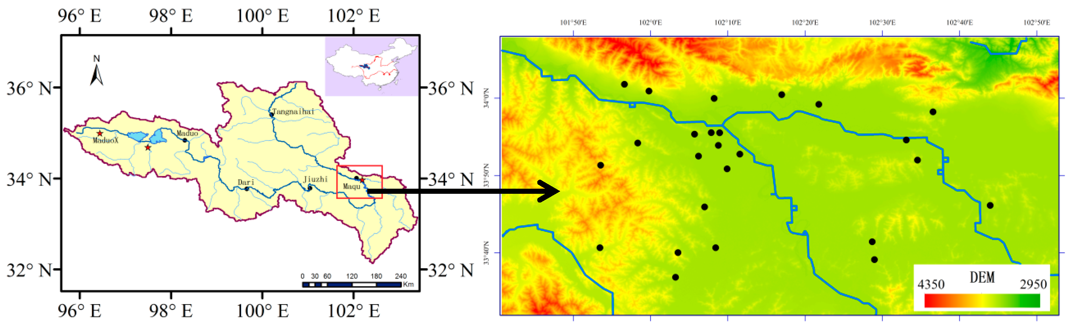
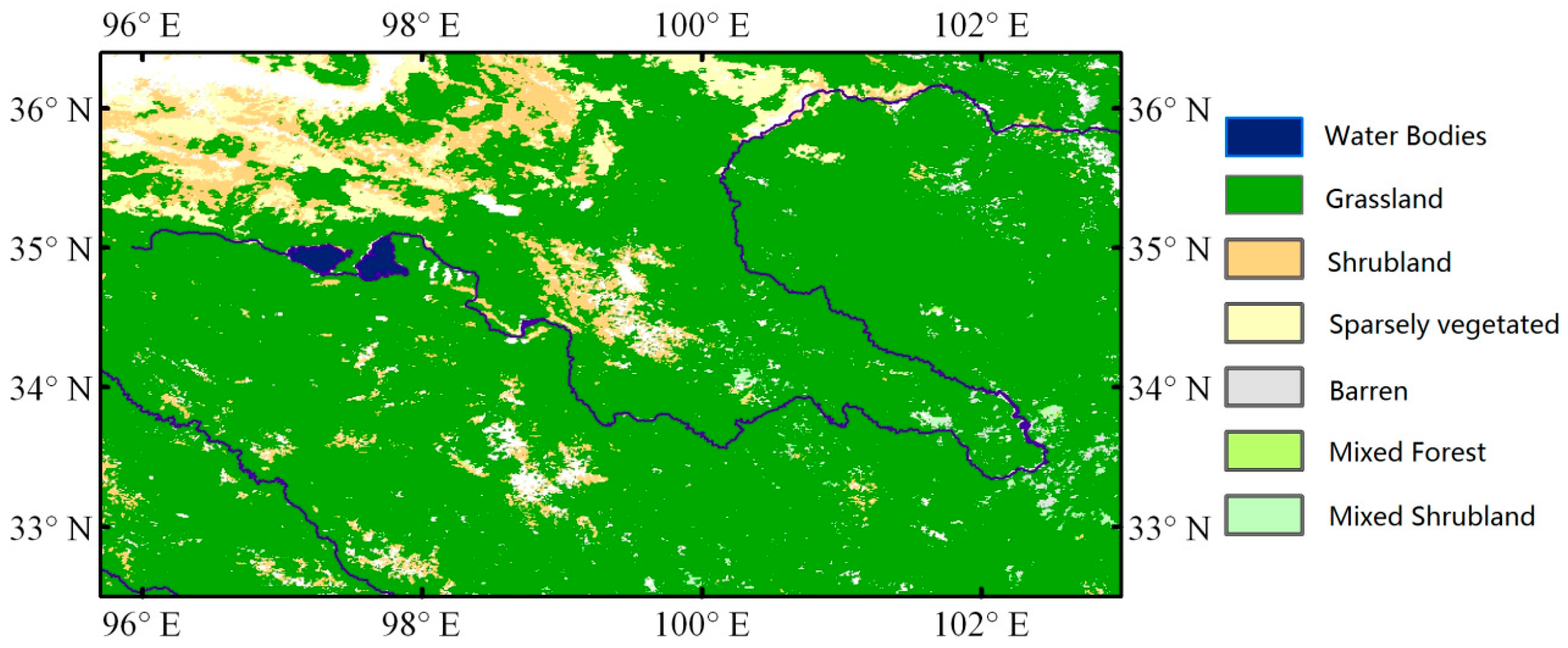
3.1. Study Area

The Yellow River source region is located in the northeastern Tibetan Plateau of 95°30′-103°30′E and 31°30′–36°30′N (Figure 1) and has an area of approximately 122,000 km². The six stations represent different catchments in the Yellow River source region. MaduoX and Maduo represent the headwaters of the Yellow River source region; Dari, Jiuzhi, and Maqu are considered the primary runoff stations; and Tangnaihai is a typical station located at the outlet of the Yellow River source region. The terrain in the region is generally high in the west and low in the east, and the most areas are above the elevation of 3000–5000 m. The annual averaged temperatures in the source region are ~1.2 °C, and generally low in the west and high in the east, representing the typical continental climate of the plateau. The annual rainfall is 250–750 mm and mainly concentrated in June–September [27]. The land use in the region is generally a weathered and broken layer of sandy bedrock covered by a thick layer of black soil and a large amount of pebbles. The soil type includes alpine meadow soil and brown calcareous soil. The two blue regions in the upper left corner of Figure 1 denote Gyaring Lake and Ngoring Lake (97°02′–97°55′E and 34°48′–35°01′N), respectively.

The vegetation type (Figure 2) in the entire source region of the Yellow River is dominated by grass with sporadic shrubs on the plateau, which are characterized by a uniform land cover of short grassland used for grazing by sheep and yaks. The terrestrial pattern can be identified according to the digital elevation model. Sporadic shrubs dominate the areas in the top and middle elevations above 4200 m.

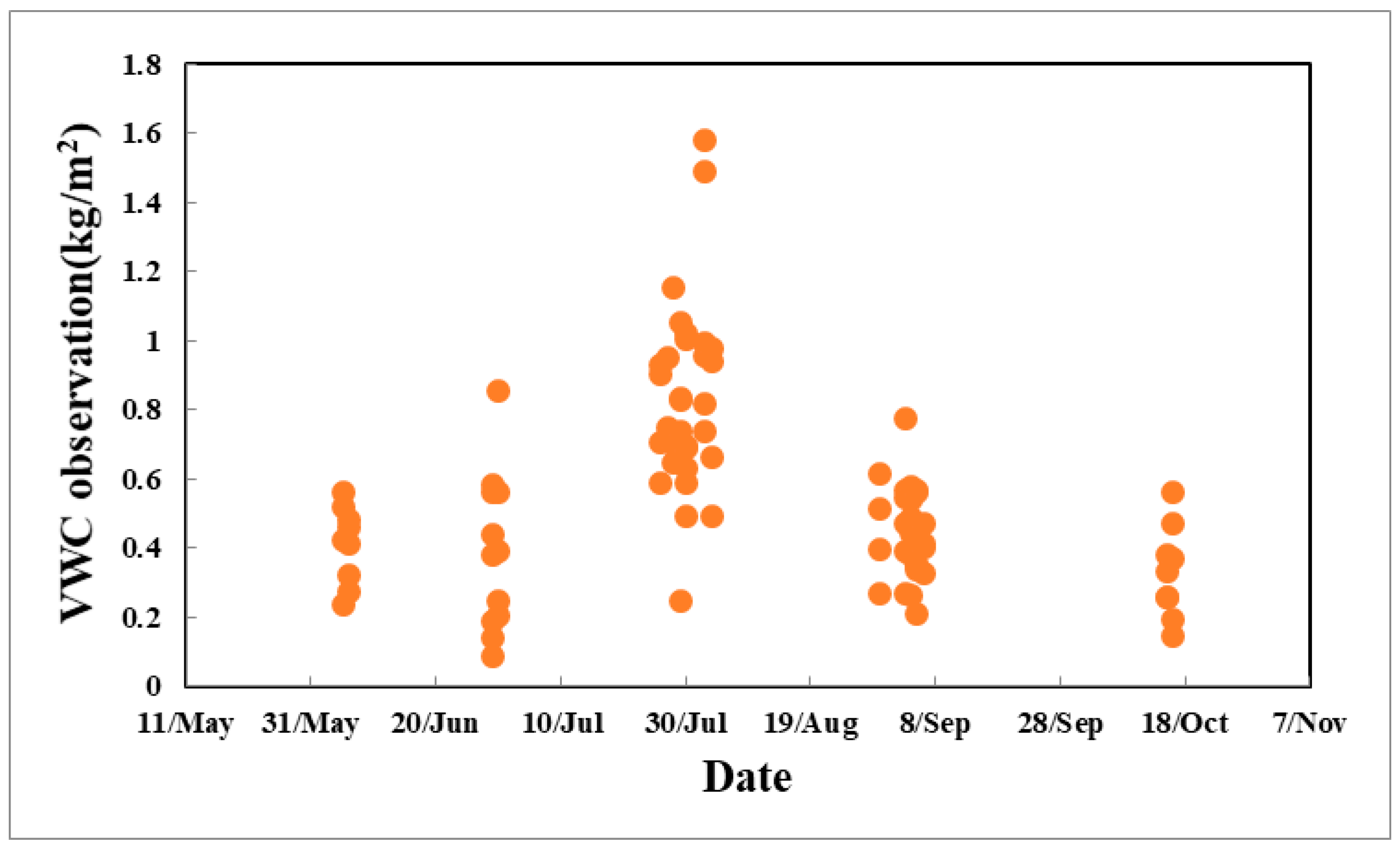
3.2. Field Observation Data

Ground measurements are critical, and a large number of point measurements can be able to provide adequate and accurate vegetation information at relevant scales. However, there are only a few such datasets available from specific field campaigns for a limited range of land cover types. Due to the coarse resolution passive microwave measurements at tens of kilometers, and twenty sampling sites in the Maqu regional scale soil moisture and soil temperature (SMST) monitoring network are selected to collect vegetation samples. Figure 1 also gives the locations and names of the monitoring sites, and the 20 sites chosen for vegetation samples which are spread over the large valley of the Yellow River. There are 11 monitoring stations installed around the valleys of the Yellow and Black Rivers, three stations in the valleys between the hills in the eastern part of the area, four stations on hill slopes, and two stations on wetlands. The vegetation samples covers an area of approximately 80 km × 80 km and the site locations are selected in order to monitor the area extensively for various altitudes and slopes. Usually, the measurements obtained at points or at very high resolutions are not comparable to the spatial scale of the passive microwave satellite measurements. In this study, the total number of stations installed in the study area are considered to be a good match between the need for sample vegetation characteristics over a wide area (covering at least one resolution cell of the satellite-derived products), and practical limitations, such as the constraints of cost and time for installation and site revisits [37]. To exclude the interference of snow and frozen water from the microwave signal, the period from early-June to mid-October is used as the experimental period. Each site is collected five times so it can basically reflect the vegetation growth in the source region from summer to early-fall. Unfortunately, five samples were scorched by misoperation. So, a total of 95 samples are obtained during the entire experiment period, including a total of 87 samples from the monitoring network, and eight samples from the source region in Maduo and MaduoX (Figure 1) required for validation. In order to improve measurement accuracy, convenience of transportation to the sites must be considered to ensure that the collected vegetation can be immediately sent back to the base station to be weighed and dried to avoid any loss of VWC.

The transit time of FY-3B over the study region was approximately 13:40 to 14:00 at local time, and the time of sampling was synchronous with the transit time of the satellite. For all the observation sites, we measured the vegetation wet weight, coverage, and height within one area unit. However, the rainy season for the study area is summer, and when it rains, the stomata of leaves open and raindrops would adhere to vegetation, causing inaccurate measurements. Therefore, the surface observations in this kind of experiments were processed under clear skies and good weather conditions when the satellite orbited over the sites. As a result, the field observations have strong representativeness.

Destructive above-ground biomass samples were collected in 30 cm × 30 cm. The location coordinates, name, number of strains, height, coverage, the soil dry–wet and weather conditions, and growth of the plant strain were also recorded. The surface dew was processed with a silica-gel desiccant and then rapidly loaded into a sealed bag with negligible weight. The bag labeled with the vegetation type, sampling time, and sampling site location was immediately returned to the laboratory for measuring fresh weight. The temperature was first fixed at 105 °C for 15 minutes and then adjusted to 80 °C for 1–2 days, and then the above-ground biomass were oven dried to a constant weight after which the dry weight was determined.

At all sampling sites, the meadow grew rapidly during the experimental period. The temporal variation of VWC within a square meter region is shown in Figure 3. The overall change of water content indicates increase first and then decrease. From late-May to mid-July, the VWC changes from 0.2kg/m² to approximately 0.8 kg/m², and it reaches the maximum of approximately 1.6 kg/m² in late-July and then continuously decreases from early-August to early-October. Consequently, VWC becomes approximately 0.5 kg/m² in early-October, although the value of certain individual measurements continues to decrease. For example, the value on June 30 is obviously lower than that on several days before. The log indicates that the weather in the study region was continuously dry, so the surface was dry. Dry weather over three continuous days produced dry soil. Soil moisture has a significant impact on the absorption systems of vegetation and the stomata closure of leaves. The overall VWC first increases and then decreases, and the vegetation growth in later months were slow because the vegetation became matured.

3.3. Remote Sensing Data

MWRI is a microwave radiometer onboard on the FY-3B satellite platform which is Chinese second-generation polar-orbiting meteorological satellites with local solar time 01:40 am (descending)/13:40 pm (ascending) orbit equatorial crossings [38]. The MWRI sensor measures vertically (V) and horizontally (H) polarized Tb at five frequencies (10.7, 18.7, 23.8, 36.5, and 89.0 GHz). The corresponding sub-stellar spatial resolutions are 51 km × 85 km, 30 km × 50 km, 27 km × 45 km, 18 km × 30 km, and 9 km × 15 km, respectively [39].

Table 1. Spectral characteristics of the Microwave Radiation Imager (MWRI).

Frequencies (GHz)	10.65	18.7	23.8	36.5	89
Polarization	V.H	V.H	V.H	V.H	V.H
Bandwidth (MHz)	180	200	400	900	2 × 2300
Calibration accuracy (K)	1.0	2.0	2.0	2.0	2.0
Spatial resolution (km × km)	51 × 85	30 × 50	27 × 45	18 × 30	9 × 15
Swath width (Km)	1400

gives the main parameters.

Few studies have been conducted about the vegetation detection by using the FY-3B microwave data sets [26,29,37]. To examine if the FY-3B MWRI has a capacity to catch the vegetation signals and obtain more accurate information on seasonal vegetation growth in the source region of the Yellow River, we use FY-3B MWRI 18.7 GHz (K band) brightness temperatures provided by the National Satellite Meteorological Center and other ancillary data inputs to derive the VOD and VWC. The daily VOD retrievals are temporally composited into 16-day median values to coincide with MODIS NDVI and MVI (see Section 4.3.2), respectively. VOD retrievals at lower (e.g., 6.9 and 10.7 GHz) microwave frequencies are reported to increase potential VOD sensitivity at higher biomass levels and sensitive to soil moisture at lower VOD levels. However, the brightness temperatures at lower frequency (≤18.7 GHz) are susceptible to radio frequency interference (RFI) mainly from surface and space-based telecommunications, so they were masked by employing frequency and polarization thresholds [18]. The channel at 18.7 GHz used in this study has low RFI and reduced atmosphere and soil moisture sensitivity relative to other channels [6].

4. Results and Discussion

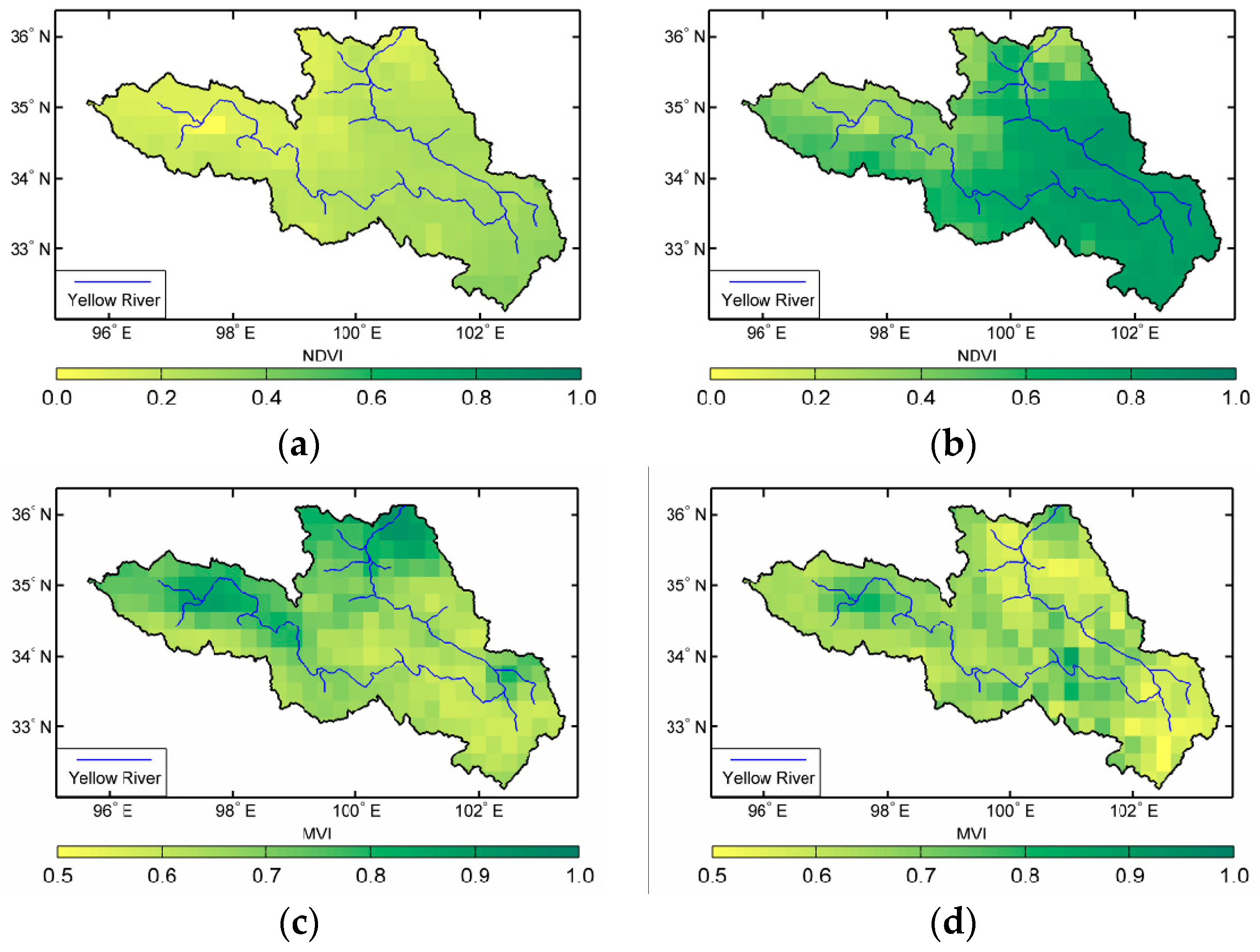
4.1. Spatial Distribution of 16-Day Mean NDVI and MVI

The 16-day composited NDVI is selected from Moderate Resolution Imaging Spectroradiometer (MODIS) data. The FY-3B MWRI is derived from MVI by using the frequency pair in 10.65 GHz and 18.7GHz [40]. Mean values of the NDVI are approximately 0.30 and 0.65 during the spring and summer seasons, respectively. For both seasons, the NDVI exhibits high values in the southern parts and low values in the northwest of the study region. The patches in the east and south parts of the study region with high NDVI values are identified as the meadow. The minimum value is located in the northwest of the study region where the Gyaring Lake and Ngoring Lake located. MVI is affected only by the vegetation properties and is negatively correlated to NDVI. Compared with the NDVI (Figure 4a,b), the corresponding MVI (Figure 4c,d) shows a great negative which exhibits lower values in the southern part and higher values in the northwest of the study region. However, the MVI exhibits obviously spatial difference especially during the summer season (Figure 4d). This demonstrates that the influence of vegetation on microwave signals also increases as the vegetation density increases. MVI can provide information on vegetation water content, structure and biomass which is complementary to that provided by NDVI.

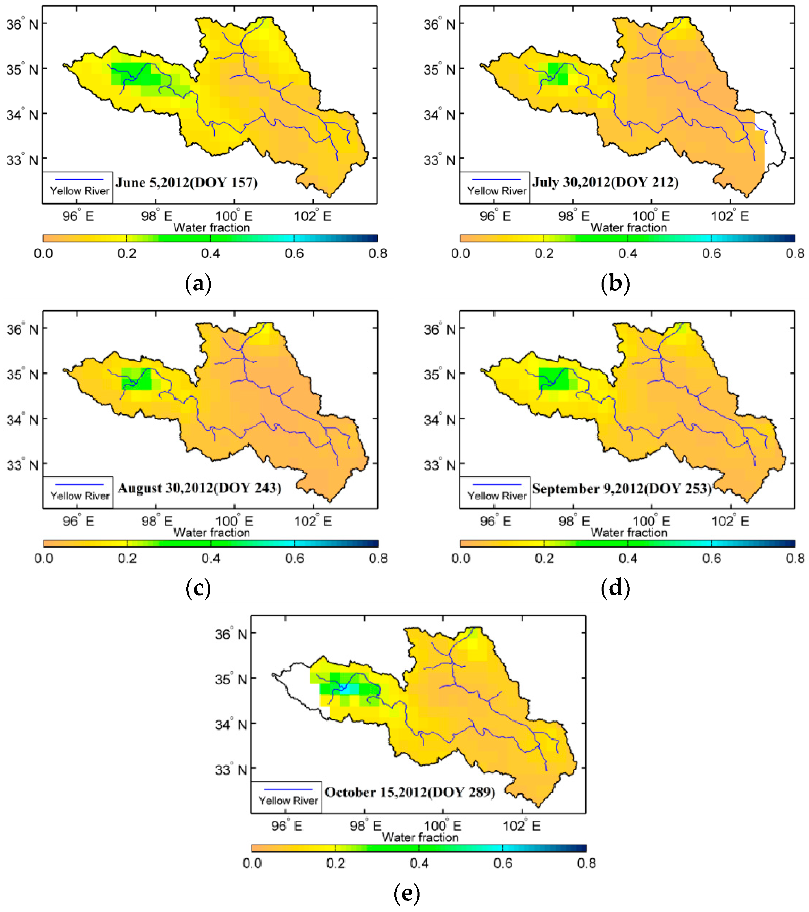
4.2. Fractional Coverage of Open Waterbodies

The underlying surface in the source region of the Yellow River includes seasonal wetland coverage. Therefore, to investigate spatial variations in VOD and VWC with considering seasonal wetland coverage, Equations (3) and (4) are combined to derive spatial distribution of fractional coverage of open water on June 5, July 30, August 30, September 9, and October 15, separately (Figure 5). Figure 5 shows that the waterbodies during the experimental period were mainly distributed in the area from the source region of the Yellow River to Maqing. In particular, the variation in fractional coverage of open water in the surrounding area of Gyaring Lake and Ngoring Lake was large (0.20–0.40), whereas the variation in the area along the Yellow River was in the range of 0.15 to 0.20. Over the whole of study region, the fractional coverage of open water in early-June and mid-October was lower than that in the other months, and the value was the highest and most obvious in late-August. The algorithm assumes that a given grid cell is composed of a mixture of open water and vegetated land, but does not specifically account for inundated pixels with overlying vegetation. Thus, the accuracy of the effective surface emissivity is improved by considering the fractional coverage of open waterbodies. Moreover, this method can be used for monitoring the composition of surface-exposed waterbodies on the scale of low-frequency microwave radiometer, and providing a basis for studying variation in the seasonal wetland in the source region of the Yellow River.

4.3. VOD Retrievals

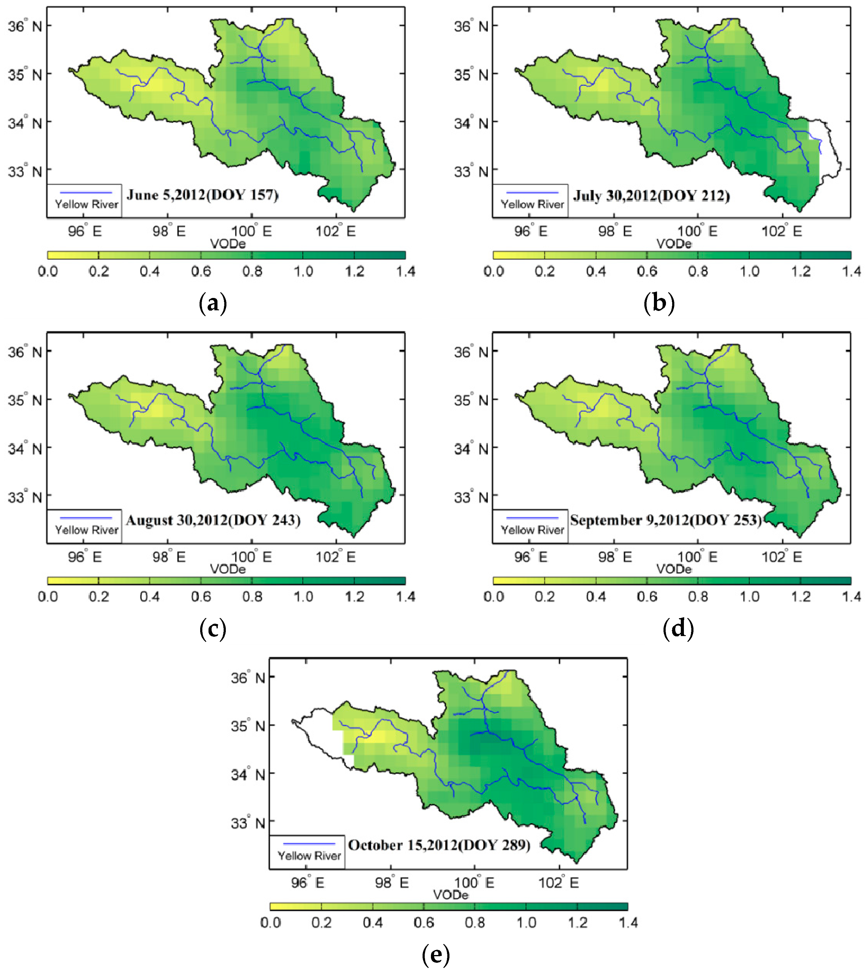
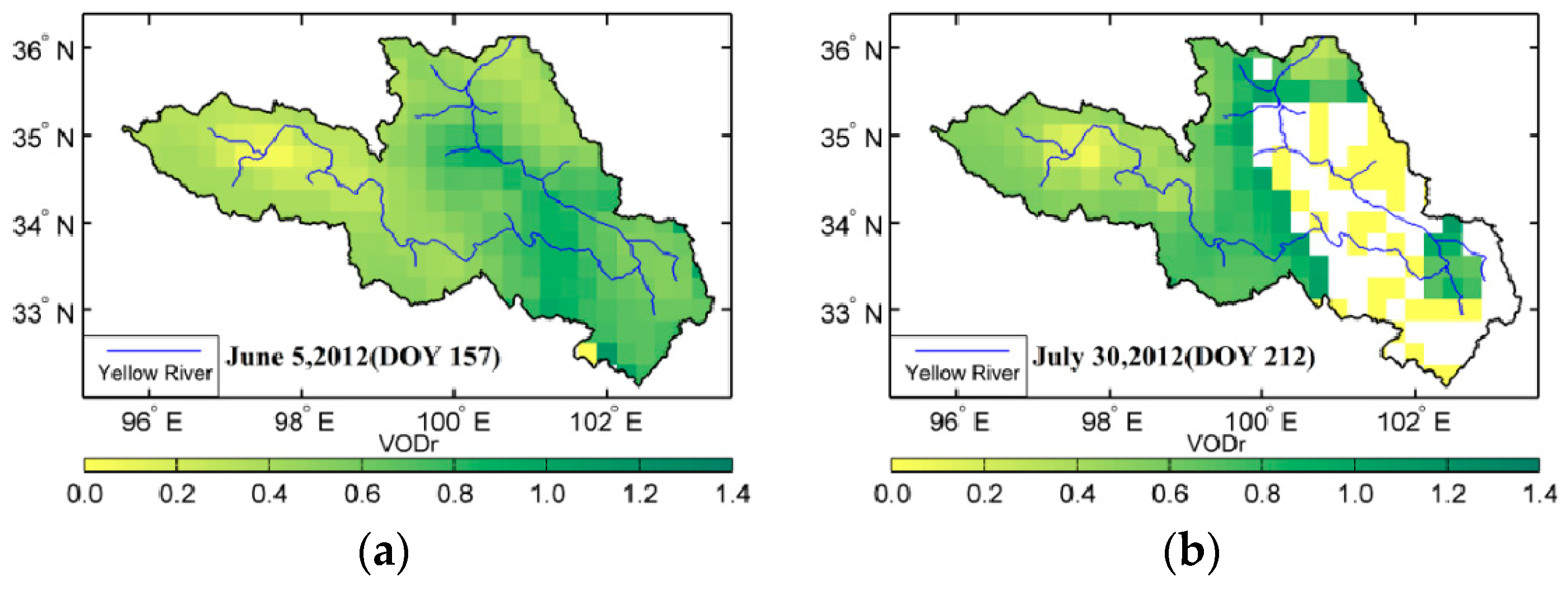
4.3.1. Spatial Variation of Retrieved VOD

To determine whether the VOD model is beneficial for analyzing waterbodies, Figure 6 and Figure 7 present the spatial distribution of VOD in the source region of the Yellow River in summer, including the results with and without the influence of waterbodies. VODr represents the VOD without the influence of waterbodies, namely, the reference VOD, and VODe represents the VOD considering the influence of waterbodies. Unlike VWC or soil moisture, VOD can not be observed or verified directly by field work. As shown in the Figure 6 and Figure 7, the results from both methods exhibit obvious seasonal changes. High-value distributions occurred along the Yellow River, where they varied in the range of 0.60 to 1.00 and generally exhibited a pattern of low in the west and high in the east. Over some part of the area, compared with these two figures, VOD without considering the contribution of waterbodies cannot obtain any results in Figure 7b–d. This demonstrates that during the period from July to September, the results from the previous method are poor in some part of the region, while the algorithm with considering waterbodies gives better results. This also means the VOD method without considering the influence of waterbodies is invalid and failed in some area at least in this study.

For the spatial distribution of VOD with considering the influence of waterbodies, the high-value region mainly occurred in the area along the Yellow River in the eastern source region and in the Tibetan Autonomous Prefecture of Aba in the southeastern source region, whereas the low-value region could be seen in the western Yellow River source region, especially in the west of Maqing. In particular, in the region from the west of Maqing to the east of Ngoring Lake, the VOD variation was obvious, with strong monthly variation. Another region with dramatic variation appeared in the east of the source region where the water content and temperature conditions were the decisive factors for vegetation growth, which indicates that the vegetation in this area was sensitive to surface temperature and moisture. The distribution of the VOD without considering the influence of waterbodies indicates that in addition to the derivation error of optical depth caused by errors in the soil moisture and temperature data, waterbodies could also interfere with the results if there was surface water in the mixed pixels, especially near Gyaring Lake and Ngoring Lake in the source region of the Yellow River. If the τ-ω model is used to retrieve VOD, the waterbodies in the mixed pixels would produce a small VOD because the application of a simplified surface radiation transfer equation cannot exclude the influence of waterbodies.

Since the surface cover in the source region of the Yellow River is dominated by alpine meadow and the coverage type is simple, the spatiotemporal distribution type of the VOD that includes the influence of waterbodies may be characterizes the seasonal timing of vegetation growing seasons, canopy growth and senescence. The timing, rate and duration of these events are vital on vegetation photosynthesis, carbon sequestration and land–atmosphere water and energy exchange. Therefore, in addition to acting as a criterion for evaluating the optical depth in the derivation of soil moisture, VOD may be used as a characteristic variable of the vegetation to characterize comprehensive features of vegetation canopy.

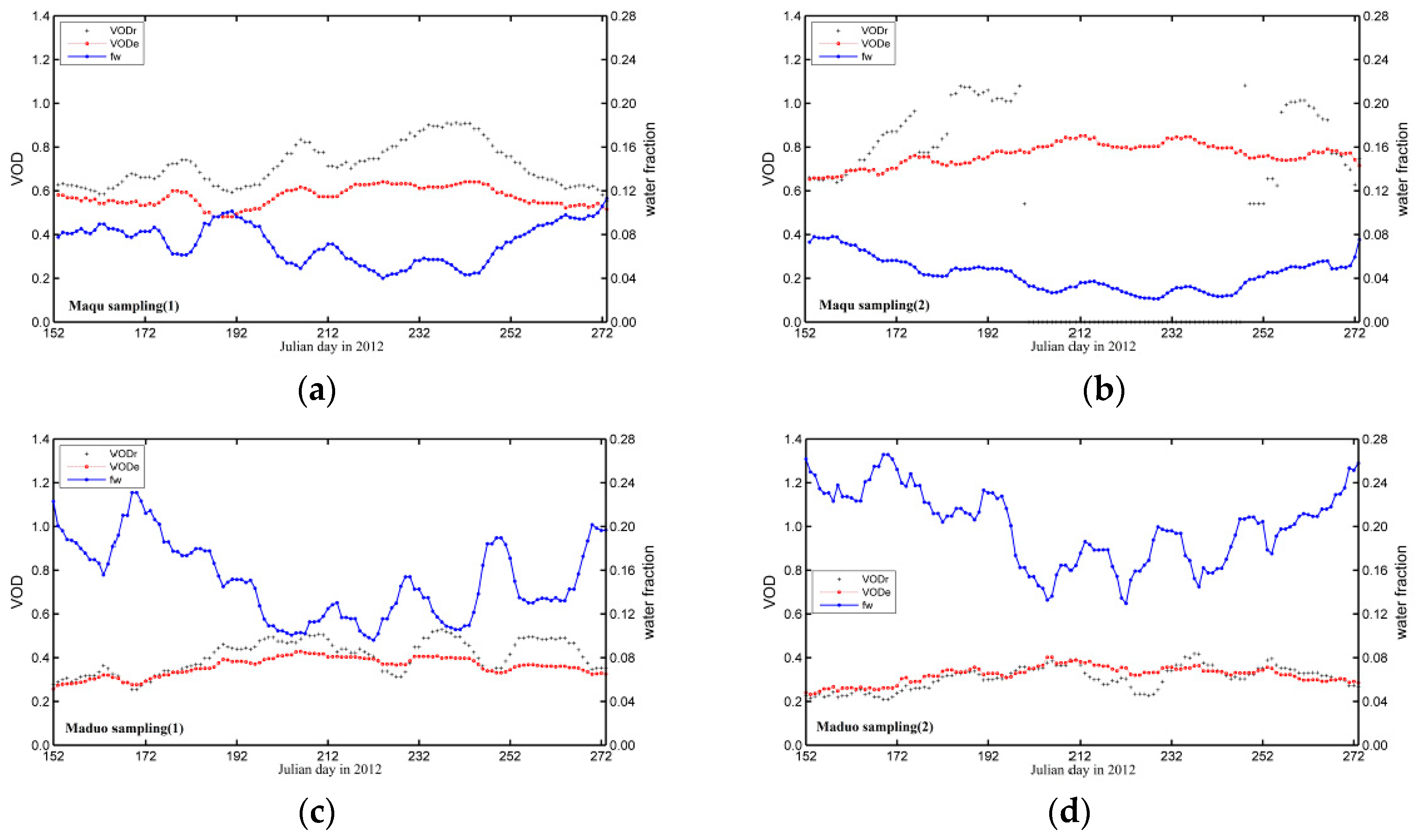
4.3.2. Temporal Variation of Retrieved VOD

To analyze the seasonal variation trend of VOD, two representative regions are selected in the study area: One is the Maqu area representing the southern part and the other is the Maduo area representing the northwest part. The fresh vegetation bag labeled with the vegetation type, sampling time must be immediately returned to the laboratory and both the sites have the laboratories for measuring and drying fresh vegetation. In each representative area, two representative sampling sites separated by 30 km are selected. Figure 8 shows the temporal distribution of the VOD at four selected sampling sites. The VODr (gray trend line) and VODe (dot-dashed red line) represent the variation trends of the algorithm with and without the influence of waterbodies, respectively. The blue line represents the temporal variation trend of water-body coverage. In the Maqu area or the Maduo area of Sister Lake, the VOD variation with including the influence of waterbodies is small and stable, indicating less interference from the waterbodies. In the Maqu area, during a period from early-June to late-September, the VOD change with considering waterbodies is smaller than that without considering waterbodies, so the former is stable. The maximum VOD appears in early-August, and is approximately 0.60. Because of high elevation of the Maduo area, the temperature and the vegetation density of the meadow are low, VOD is small, and the maximum VOD does not exceed 0.40. Moreover, the variation in the Maduo area is less obvious than that in the Maqu area. The seasonal trend of water-body coverage is consistent in the same region. In the source region, because the water coverage in Sister Lake is abundant, the water-body coverage shows higher than that in the Maqu area. In addition, the algorithm fails obtaining VOD at one site of Maqu without considering the influence of waterbodies.

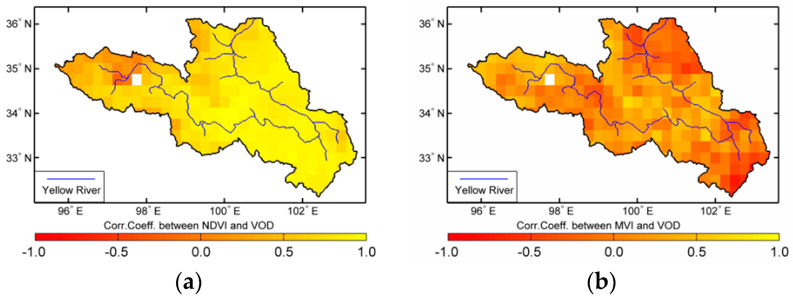
4.3.3. Correlations between Retrieved VOD and Vegetation Indexes

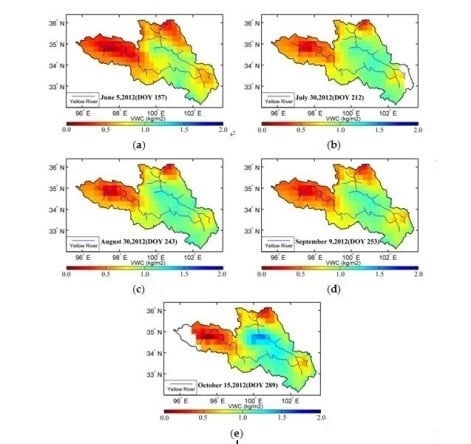
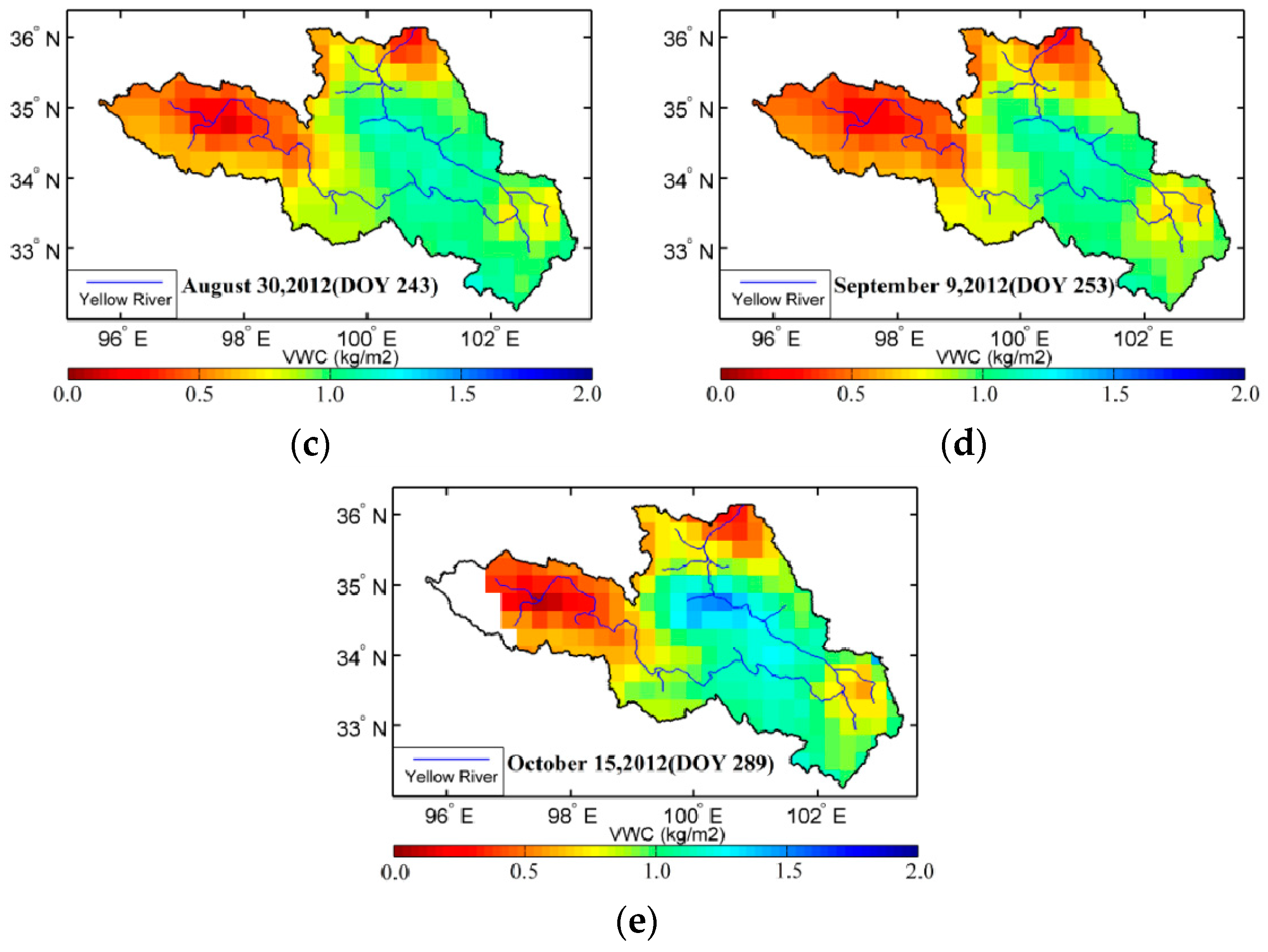
The VOD parameter is an indicator of canopy density and VWC, while NDVI is directly related to the photosynthetic canopy cover and mainly depends on green leaf material of the vegetation cover. MVI includes information of both leafy and woody parts of vegetation because of greater penetration and sensitivity. The ranked Spearman correlation coefficients [20] between retrieved VOD against NDVI or MVI during the experimental period are given in Figure 9. These metrics are potentially complementary and together provide a more comprehensive VOD assessment. While we might expect a favorable, positive correlation between VOD and NDVI time series, negative correlation between VOD and MVI time series in Figure 9. Here, the interferences from Gyaring and Ngoring Lake on these statistics are not considered. As shown in Figure 2, the distribution patterns of the vegetation index derived from the optical and microwave sensors exhibits a good correlation with the land cover type. Land cover categories with characteristically high biomass levels show the highest correlations, with decreasing correspondence for land cover classes with characteristically lower canopy density and biomass. It shows that there is a significant positive correlation between NDVI and VOD in the eastern part of the source region of the Yellow River, but the positive correlation becomes gradually weak in the northwest of the study area. The correlation becomes zero near the boundary areas. In the east part of the study area, the values of correlation between NDVI and VOD can reach 0.8 to 1.0, but the correlation is going to descend in the northwest especially around the two lakes. The strong negative correlations between MVI and VOD are occurred in the east and north part, and the values can reach −0.5 to −0.9. There are many factors that may contribute to correlations between VOD and vegetation index in the study. The fractions of uneven terrain, wet and mixed snow, ice cover and frost cover are found to reduce the correlation. The MVI shows a significant large negative correlation with the VOD in the northwest and southeast of the source region area. Figure 9 indicates that both NDVI and MVI have a strong correlation with VOD, so they can be considered as characteristic variables for monitoring VOD variation during the vegetation growing season. Nevertheless, in the middle of source region NDVI reflects the VOD more reasonable variation than MVI does because of the impact of land cover.

4.4. VWC Retrievals

Although VOD is usually assumed to be linearly proportional to VWC [32], a good logarithmic correspondence between these two parameters is obtained in this study. Figure 10 (black line represents logarithm trend line) presents logarithmic function between VOD and VWC, there is a good corresponding relationship between VWC and VOD in the source region during the summer season. According to the Figure 10, the parameter b is determined by the logarithm trend line $y=1.5524\ln (x)+1.5566$. With this relationship the spatial VWC is obtained during the entire growth period (Figure 11).

Since the iterative solution of the VOD directly retrieved based on the τ-ω model cannot be obtained in certain regions, we retrieve spatial distribution of the VWC in the source region with including the impact of waterbodies, as shown from Figure 11. The VWC in the entire source region indicates a variation in the range of 0.20 to 1.20kg/m², and the high VWC appears along the Yellow River and in the southeastern part where the Aba-Tibetan Autonomous Prefecture located. The VWC exhibits less seasonal variation in the western source region, especially in the area from the west of Maqing to the east of Ngoring Lake. This result indicates that the vegetation is sparse in this region, which is dominated by exposed soil. Because the water content and temperature are the most important factors for vegetation growth in the source region of the Yellow River, a large variation of 0.30 to 0.80kg/m² appears in the Maqu area to the east, indicating that the vegetation in the Maqu area is more sensitive to surface temperature and moisture. In the northern region near the Qaidam Basin, the vegetation coverage is low and the VWC value is small as well. Such of those results were found for an AMSR-E daily brightness temperature by Chen et al. [41]. That study did not specify analysis the quantitative relationship between the VOD and VWC, although a field observation and an inversion model of vegetation index is mentioned for VWC. In the current study, no statistically significant phase lags are found for any of the vegetation classes.

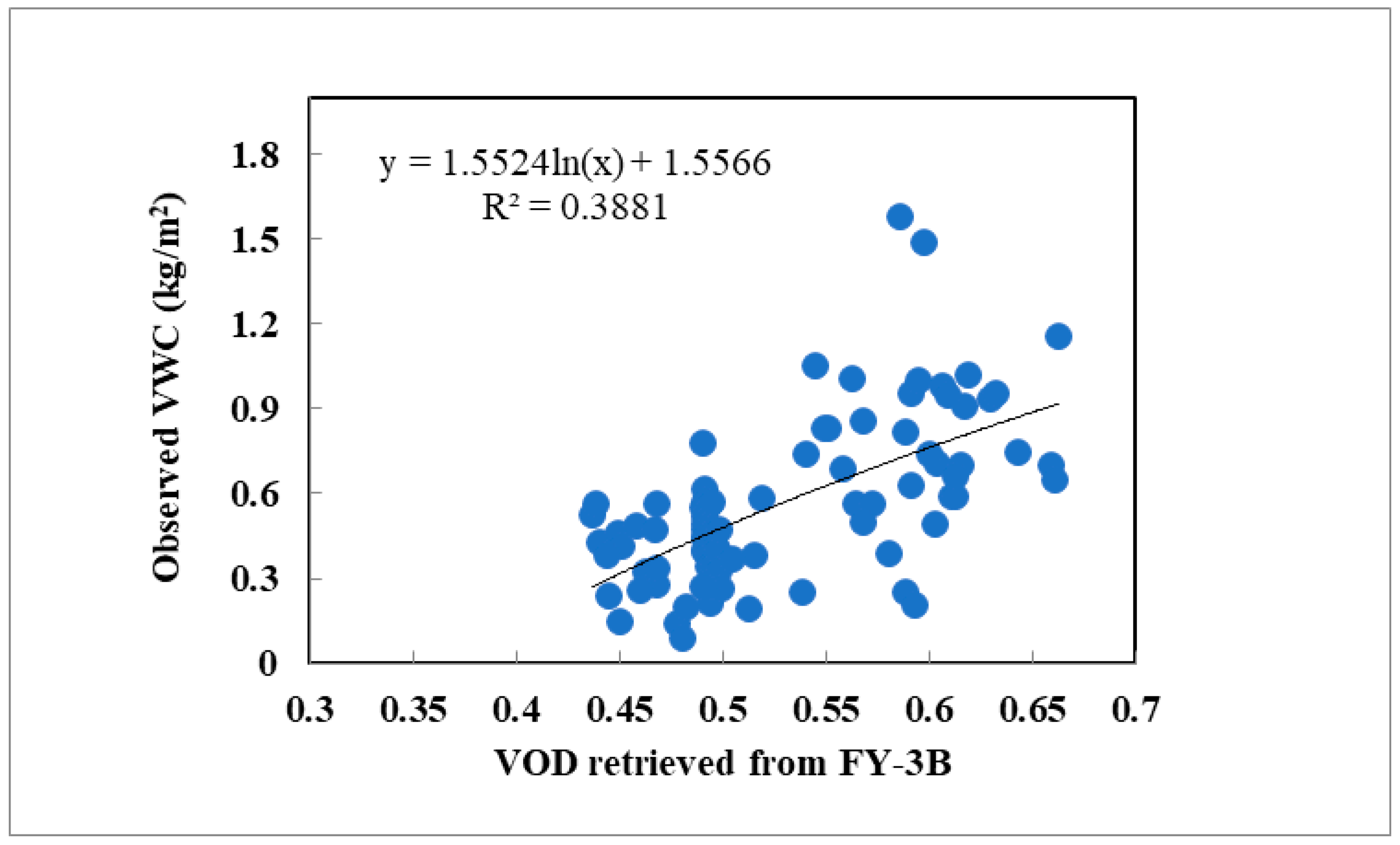
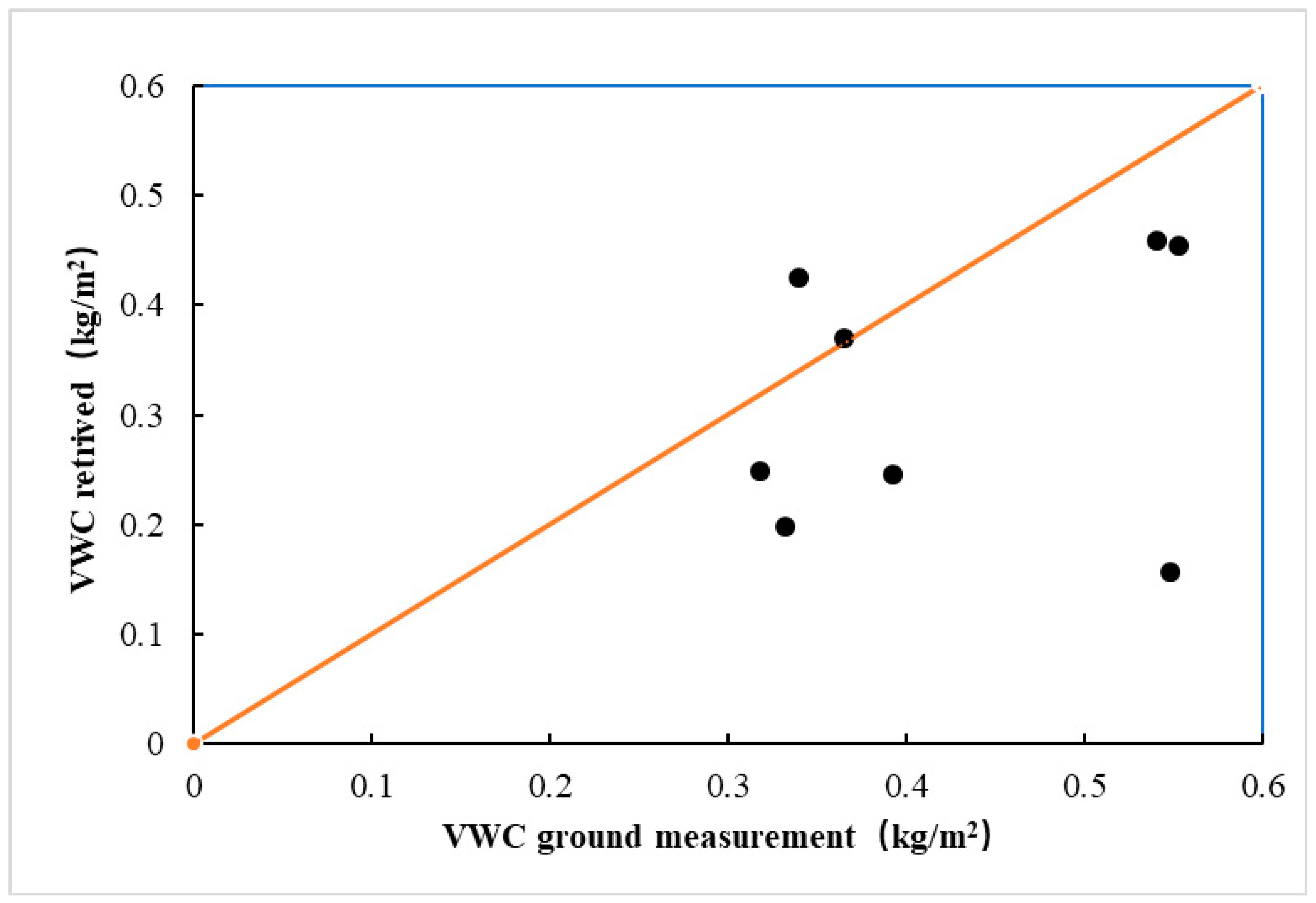
4.5. Validation of VWC

Maqu regional scale soil moisture and soil temperature monitoring network is set up in the water source region of the Yellow River to validate the accuracy of the satellite-derived soil moisture products over the Tibetan Plateau. This network has the capability to monitor the spatial and temporal soil moisture variability of the area with a high degree of accuracy [37,42]. The VWC sampling is collected according to the network site. Dente et al. [42] proposed that the weighted spatial average of measured soil moisture was successfully used as the ground reference for validation of the AMSR-E soil moisture products and ASCAT soil wetness index products. The results from Dente’s study are very encouraging for our applications. So, the match problem can be ignored in our opinion.

Figure 12 presents a comparison between the measured VWC at the sampling sites and the derived VWC from the remote sensing (red line represents reference line of zero bias). During the experimental period from early-June to mid-October, 95 samples were collected in the southern area. The validation data, however, were collected from the northwest of the region. The altitude of the northwest of the study area is more than 4200 m. Compared with the southern part, the northwest area shows a higher latitude and less vegetation cover (Figure 1 and Figure 2). Because the validation region was less affected by human activity and the road was rough, we only collected samples from four sites. The root mean square error is 0.12 kg/m². At one sampling, the value for the remote sensing retrieval was ~0.15 kg/m², but the value for the surface observation was ~0.55 kg/m². This discrepancy might have been caused by the sampling site location, which was close to the lake. Thus, the sensor likely received more signals from the waterbody than the vegetation. Figure 12 shows the retrieved VWC from the remote sensing is smaller than the measured one. The difference is resulted from the model systematic error that the non-exposed waterbodies are excluded. However, the difference may also be contributed by the fixed values of the parameters used during the iterative processes, such as the effective emissivity of vegetation. Moreover, the observation angle and transient field of the view of the sensor can also affect the model accuracy.

5. Summary and Conclusions

In this study, the τ-ω model was improved by using the dual-polarized brightness temperature observations at the K-band obtained from the MWRI microwave radiometer on board the FY-3B meteorological satellite and removing the influence of waterbodies. By constructing a microwave VOD model that is suitable for the source region of the Yellow River, one can be able to quantitatively retrieve the canopy VWC.

The VOD scheme considering the influence of waterbodies demonstrated superior to the one directly using the τ-ω model for the inversion. The VOD with considering the influence of waterbodies showed a large-value region occurring primarily in the area along the Yellow River and in the southeastern source region, where seasonal variation was dramatic. In particular, in the region from the west of Maqing to the east of Ngoring Lake, the VOD exhibited strong monthly variation. In the Maqu area, the maximum VOD of approximately 0.60 occurred in early-August. Due to low vegetation density in the source region of the Yellow River, the maximum VOD was less than 0.40.

The VWC in the entire source region was in the range of 0.20 to 1.40kg/m², and the large-value area was mainly located along the Yellow River in the eastern source region. Large variation in the source region in the range of 0.20 to 0.50 kg/m² occurred in the Maqu area to the east, whereas in the western source region it did not show seasonal variation obviously, especially in the east of Ngoring Lake.

Although the VWC was derived by using the field observations, the number of samples is still insufficient. An analytic experiment about vegetation canopy samples with an even broader coverage range is necessary if these data are employed to derive the parameter b that is suitable for variation in vegetation coverage in the source region of the Yellow River to retrieve canopy VWC.

The error analysis of VWC indicated that the τ-ω model considering the influence of waterbody coverage was reasonable for derivation of vegetation canopy characteristics in the source region of the Yellow River. This study has shown that the brightness temperature data from the MWRI sensor on board the FY-3B could be used for land surface parameters retrieval in the source region of the Yellow River.

References

1. Colliander, A.; Cosh, M.H.; Misra, S.; Jackson, T.J.; Crow, W.T.; Chan, S.; Bindlish, R.; Chae, C.; Collins, C.H.; Yueh, S.H. Validation and scaling of soil moisture in a semi-arid environment: SMAP validation experiment 2015 (SMAPVEX15). Remote Sens. Environ. 2017, 196, 101–112. [Google Scholar] [CrossRef]
2. Yi, L.; Zhang, W.C.; Li, X.Y. Assessing hydrological modelling driven by different precipitation datasets via the smap soil moisture product and gauged streamflow data. Remote Sens. 2018, 10, 1872. [Google Scholar] [CrossRef]
3. Njoku, E.G.; Chan, S.K. Vegetation and surface roughness effects on AMSR-E land observations. Remote Sens. Environ. 2006, 100, 190–199. [Google Scholar] [CrossRef]
4. Du, J.Y. A method to improve satellite soil moisture retrievals based on Fourier analysis. Geophysi. Res. Lett. 2012, 39. [Google Scholar] [CrossRef]
5. Talebiesfandarani, S.; Zhao, T.J.; Shi, J.C.; Ferrazzoli, P.; Wigneron, J.P.; Zamani, M.; Pani, P. Microwave vegetation index from multi-angular observations and its application in vegetation properties retrieval: Theoretical modelling. Remote Sens. 2019, 11, 730. [Google Scholar] [CrossRef]
6. Njoku, E.G.; Li, L. Retrieval of land surface parameters using passive microwave measurements at 6–18 GHz. IEEE Trans. Geosci. Remote Sens. 1999, 37, 79–93. [Google Scholar] [CrossRef]
7. Kolassa, J.; Gentine, P.; Prigent, C.; Aires, F. Soil moisture retrieval from AMSR-E and ASCAT microwave observation synergy. Part 1: Satellite data analysis. Remote Sens. Environ. 2016, 173, 1–14. [Google Scholar] [CrossRef]
8. Liu, Y.Y.; van Dijk, A.I.J.M.; de Jeu, R.A.M.; Canadell, J.G.; McCabe, M.F.; Evans, J.P.; Wang, G. Recent reversal in loss of global terrestrial biomass. Nat. Clim. Chang. 2015, 5, 470–474. [Google Scholar] [CrossRef]
9. Jones, M.O.; Kimball, J.S.; Jones, L.A.; McDonald, K.C. Satellite passivemicrowave detection of North America start of season. Remote Sens. Environ. 2012, 123, 324–333. [Google Scholar] [CrossRef]
10. Barichivich, J.; Briffa, K.R.; Myneni, R.B.; Osborn, T.J.; Melvin, T.M.; Ciais, P.; Piao, S.; Tucker, C. Large-scale variations in the vegetation growing season and annual cycle of atmospheric CO2 at high northern latitudes from 1950 to 2011. Glob. Chang. Biol. 2013, 19, 3167–3183. [Google Scholar] [CrossRef]
11. Marle, M.V.; Werf, G.V.D.; Jeu, R.D.; Liu, Y. Annual South American forest loss estimates based on passive microwave remote sensing (1990–2010). Biogeosciences 2016, 13, 609–624. [Google Scholar] [CrossRef]
12. Miralles, D.G.; Holmes, T.R.H.; De Jeu, R.A.M.; Gash, J.H.; Meesters, A.G.C.A.; Dolman, A.J. Global land-surface evaporation estimated from satellite-based observations. Hydrol. Earth Syst. Sci. 2011, 15, 453–469. [Google Scholar] [CrossRef] [Green Version]
13. Miralles, D.G.; Nieto, R.; McDowell, N.G.; Dorigo, W.A.; Verhoest, N.E.; Liu, Y.Y.; Teuling, A.J.; Dolman, A.J.; Good, S.P.; Gimeno, L. Contribution of water-limited ecoregions to their own supply of rainfall. Environ. Res. Lett. 2016, 11, 124007. [Google Scholar] [CrossRef]
14. Jones, M.O.; Jones, L.A.; Kimball, J.S.; Mcdonald, K.C. Satellite passive microwave remote sensing for monitoring global land surface phenology. Remote Sens. Environ. 2011, 115, 1102–1114. [Google Scholar] [CrossRef]
15. Meesters, A.; De, J.R.; Owe, M. Analytical derivation of the vegetation optical depth from the microwave polarization difference index. IEEE Geosci. Remote Sens. 2006, 2, 121–123. [Google Scholar] [CrossRef]
16. Shi, J.C.; Jiang, L.M.; Zhang, L.X.; Chen, K.S.; Wigneron, J.P.; Chanzy, A.; Jackson, T.J. Physically based estimation of bare-surface soil moisture with the passive radiometers. IEEE Trans. Geosci. Remote Sens. 2006, 44, 3145–3153. [Google Scholar] [CrossRef]
17. Shi, J.C.; Jackson, T.J.; Tao, J.; Du, J.; Bindlish, R.; Lu, L.; Chen, K.S. Microwave vegetation indices for short vegetation covers from satellite passive microwave sensor AMSR-E. Remote Sens. Environ. 2008, 112, 4285–4300. [Google Scholar] [CrossRef]
18. Njoku, E.G.; Ashcroft, P.; Chan, T.K.; Li, L. Global survey and statistics of radiofrequency interference in AMSR-E land observations. IEEE Trans. Geosci. Remote Sens. 2005, 43, 938–947. [Google Scholar] [CrossRef]
19. Jones, L.A.; Ferguson, C.R.; Kimball, J.S.; Zhang, K.; Chan, S.T.K.; McDonald, K.C.; Njoku, E.G.; Wood, E.F. Satellite microwave remote sensing of daily land surface air temperature minima and maxima from AMSR-E. IEEE J. Sel. Top. Appl. Earth Obs. Remote Sens. 2010, 3, 111–123. [Google Scholar] [CrossRef]
20. Grant, J.P.; Wigneron, J.-P.; De Jeu, R.A.M.; Lawrence, H.; Mialon, A.; Richaume, P.; Al Bitar, A.; Drusch, M.; van Marle, M.J.E.; Kerr, Y. Comparison of SMOS and AMSR-E vegetation optical depth to four MODIS-based vegetation indices. Remote Sens. Environ. 2016, 172, 87–100. [Google Scholar] [CrossRef]
21. Owe, M.; Jeu, R.D.; Walker, J. A methodology for surface soil moisture and vegetation opticaldepth retrieval using the microwave polarization difference index. IEEE Trans. Geosci. Remote Sens. 2001, 39, 1643–1654. [Google Scholar] [CrossRef]
22. Gao, H.; Wood, E.F.; Jackson, T.J.; Drusch, M.; Bindlish, R. Using TRMM/TMI to Retrieve Surface Soil Moisture over the Southern United States from 1998 to 2002. J. Hydrometer. 2006, 7, 815–818. [Google Scholar] [CrossRef]
23. Oveisgharan, S.D.; Haddad, Z.; Turk, J.; Rodriguez, E.; Li, L. Soil moisture and vegetation water content retrieval using QuikSCAT data. Remote Sens. 2018, 10, 636. [Google Scholar] [CrossRef]
24. Meyer, T.; Weihermüller, L.; Vereecken, H.; Jonard, F. Vegetation Optical Depth and Soil Moisture Retrieved from L-Band Radiometry over the Growth Cycle of a Winter Wheat. Remote Sens. 2018, 10, 1637. [Google Scholar] [CrossRef]
25. Zheng, D.H.; Wang, X.; Velde, R.V.D.; Ferrazzoli, P.; Wen, J.; Wang, Z.L.; Schwank, M.; Colliander, A.; Bindlish, R.; Su, Z.B. Impact of surface roughness, vegetation opacity and soil permittivity on L-band microwave emission and soil moisture retrieval in the third pole environment. Remote Sens. Environ. 2018, 209, 633–647. [Google Scholar] [CrossRef]
26. Jackson, T.J.; Schmugge, T.J. Vegetation effects on the microwave emission of soils. Remote Sens. Environ. 1991, 36, 203–212. [Google Scholar] [CrossRef]
27. Liu, R.; Wen, J.; Wang, X.; Wang, Z.L. Validation of evapotranspiration and its long-term trends in the Yellow River source region. J. Water Clim. Chang. 2017, 8, 495–509. [Google Scholar] [CrossRef]
28. Ulaby, F.T.; Moore, R.K.; Fung, A.K. Microwave Remote Sensing, Active and Passive; Artech House: Dedham, MA, USA, 1986; p. 2. [Google Scholar]
29. Wang, J.R.; Choudhury, B.J. Remote sensing of soil moisture content over bare fields at 1.4 GHz frequency. J. Geophys. Res. 1981, 86, 5277–5282. [Google Scholar] [CrossRef]
30. Dobson, M.C.; Ulaby, F.T.; Hallikainen, M.T.; El-Rayes, M.A. Microwave dielectric behavior of wet soil-Part II: Dielectric mixing models. IEEE Trans. Geosci. Remote Sens. 1985, GE-23, 35–46. [Google Scholar] [CrossRef]
31. Holmes, T.R.H.; Drusch, M.; Wigneron, J.P.; RAMDe, J. A global simulation of microwave emission: Error structures based on output from ECMWF’s operational Integrated Forecast System. IEEE Trans. Geosci. Remote Sens. 2008, 46, 846–856. [Google Scholar] [CrossRef]
32. Jackson, T.J.; O’Neill, P.E. Attenuation of soil microwave emissivity by corn and soybeans at 1.4 and 5 GHz. IEEE Trans. Geosci. Remote Sens. 1990, 28, 978–980. [Google Scholar] [CrossRef]
33. Van De Griend, A.A.; Wigneron, J.P. The b-factor as a function of frequency and canopy type at H-polarization. IEEE Trans. Geosci. Remote Sens. 2004, 42, 786–794. [Google Scholar] [CrossRef]
34. Jackson, T.J.; Le Vine, D.M.; Hsu, A.Y.; Oldak, A.; Starks, P.J.; Swift, C.T.; Ishan, J.D.; Haken, M. Soil moisture mapping at regional scales using microwave radiometry: The Southern Great Plains Hydrology Experiment. IEEE Trans. Geosci. Remote Sens. 1999, 37, 2136–2151. [Google Scholar] [CrossRef]
35. Jackson, T.J.; Hsu, A.Y.; O’Neill, P.E. Surface Soil Moisture Retrieval and Mapping Using High-Frequency Microwave Satellite Observations in the Southern Great Plains. J. Hydrometer. 2002, 3, 688–699. [Google Scholar] [CrossRef]
36. English, S.J. The importance of accurate skin temperature in assimilating radiances from satellite sounding instruments. IEEE Trans. Geosci. Remote Sens. 2008, 46, 403–408. [Google Scholar] [CrossRef]
37. Zheng, D.H.; Wang, X.; van der Velde, R.; Zeng, Y.; Wen, J.; Wang, Z.; Schwank, M.; Ferrazzoli, P.; Su, Z. L-Band Microwave Emission of Soil Freeze-Thaw Process in the Third Pole Environment. IEEE Trans. Geosci. Remote Sens. 2017, 99, 1–15. [Google Scholar] [CrossRef]
38. Cui, Y.K.; Long, D.; Hong, Y.; Zeng, C.; Zhou, J.; Han, Z.Y.; Liu, R.H.; Wan, W. Validation and reconstruction of FY-3B/MWRI soil moisture using an artificial neural network based on reconstructed MODIS optical products over the Tibetan Plateau. J. Hydrometer. 2016, 543, 242–254. [Google Scholar] [CrossRef]
39. Yang, J.T.; Jiang, L.M.; Shi, J.C.; Wu, S.L.; Sun, R.J.; Yang, H. Monitoring snow cover using Chinese meteorological satellite data over China. Remote Sens. Environ. 2014, 143, 192–203. [Google Scholar] [CrossRef]
40. Paloscia, S.; Pampalonil, P. Microwave vegetation indexes for detecting biomass and water conditions of agricultural crops. Remote Sens. Environ. 1992, 40, 15–26. [Google Scholar] [CrossRef]
41. Chen, S.Y.; Yu, H.; Feng, Q.S.; Liang, T.G. Dynamic monitoring of vegetation water content based on microwave remote sensing in Qinghai-Tibetan Plateau region from 2002 to 2010. Acta Prataculturae Sinica. 2013, 5, 1–10. [Google Scholar]
42. Dente, L.; Vekerdy, Z.; Wen, J.; Su, Z. Maqu network for validation of satellite-derived soil moisture products. Int. J. Appl. Earth Obs. 2012, 17, 55–65. [Google Scholar] [CrossRef]
Figure 1. Location of the source region of the Yellow River catchment (left) and Maqu soil moisture and soil temperature (SMST) monitoring network (right) [37]. (Left: red five-stars represent the sampling stations: Maqu 87 times and Maduo 8 times.).
Remotesensing 11 01536 g001
Figure 2. Land cover map in the source region of the Yellow River.
Remotesensing 11 01536 g002
Figure 3. Variation of observed vegetation water content (VWC) during the experimental period.
Remotesensing 11 01536 g003
Figure 4. Spatial distribution of 16-day mean normalized difference vegetation index (NDVI) and microwave vegetation index (MVI). (a,b) NDVI from 23 April to 8 May and 13 to 28 July, 2012, respectively. (c,d) MVI from 23 April to 8 May and 12 to 28 July, 2012, respectively.
Remotesensing 11 01536 g004
Figure 5. Spatial distribution of the fractional coverage of open waterbodies (fw) during summer of 2012.
Remotesensing 11 01536 g005
Figure 6. Vegetation optical depth (VOD) considering waterbody influence during the summer of 2012 in the source region of the Yellow River, China.
Remotesensing 11 01536 g006
Figure 7. VOD without waterbody influence during the summer of 2012 in the source region of the Yellow River, China.
Remotesensing 11 01536 g007aRemotesensing 11 01536 g007b
Figure 8. Temporal distribution of VOD in the Yellow River source region during summer 2012.
Remotesensing 11 01536 g008
Figure 9. Correlations between retrieved VOD against (a) NDVI or (b) MVI during the experimental period.
Remotesensing 11 01536 g009
Figure 10. Relationship between measured VWC and microwave-retrieved VOD in the source region of the Yellow River.
Remotesensing 11 01536 g010
Figure 11. Spatial distribution of VWC during summer of 2012 in the Yellow River source region, China.
Remotesensing 11 01536 g011aRemotesensing 11 01536 g011b
Figure 12. Comparison between the remote-sensing derived VWC and the measured VWC.
Remotesensing 11 01536 g012