Investigating the Consistency of Uncalibrated Multispectral Lidar Vegetation Indices at Different Altitudes


Abstract
1. Introduction
1.1. The Titan Spectral Vegetation Indices
1.2. Lidar Radiometry
1.3. Lidar Intensity Metrics
1.4. Angular Effects of Lidar Backscatter
1.5. Relevant Studies and Impetus for the Experiment
1.6. Hypothesis and Objectives
1.6.1. Single Channel Intensity Ratios
1.6.2. Comparison of Point Density Distributions across Three Altitudes
1.6.3. Consistency of Spectral Vegetation Indices through Different Altitudes
1.6.4. Comparing the Consistency of sρ vs. nδ
2. Data and Methods
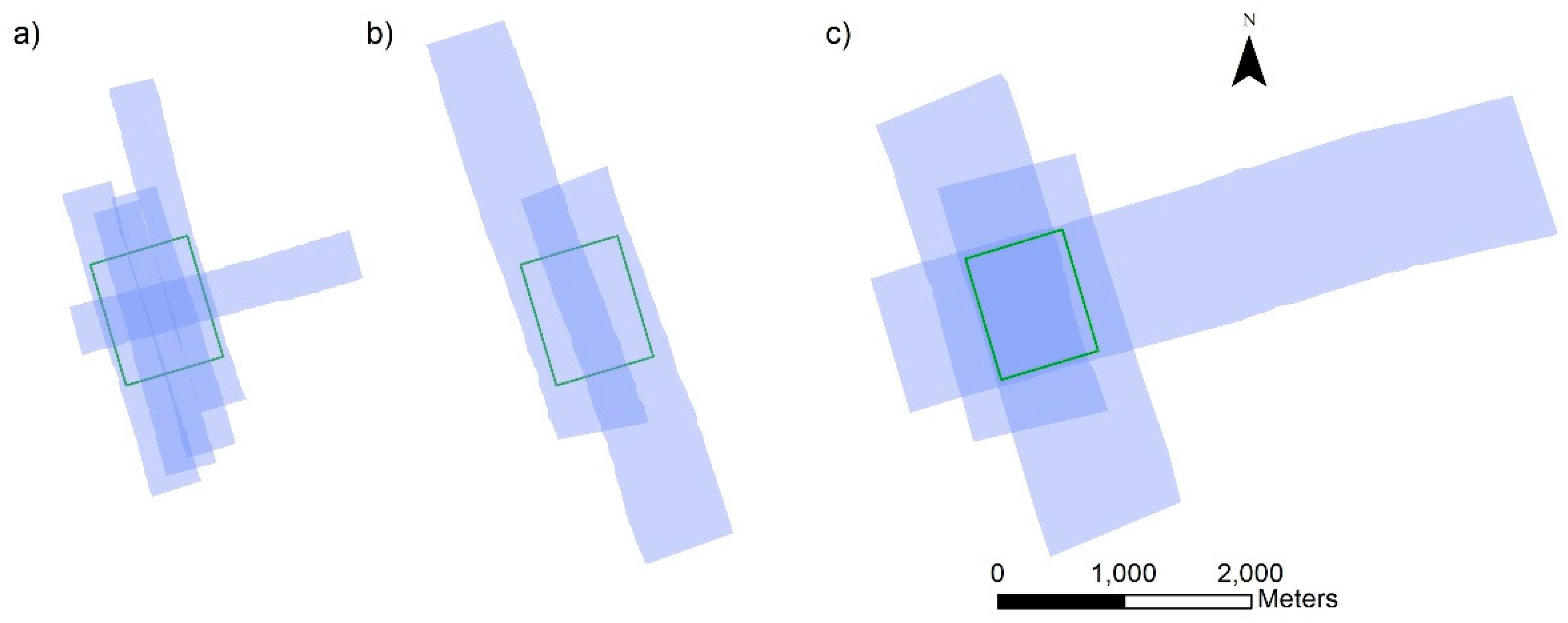
2.1. Study Area and Data Collection
2.2. Scan Line Intensity Banding
2.3. Comparative Analysis
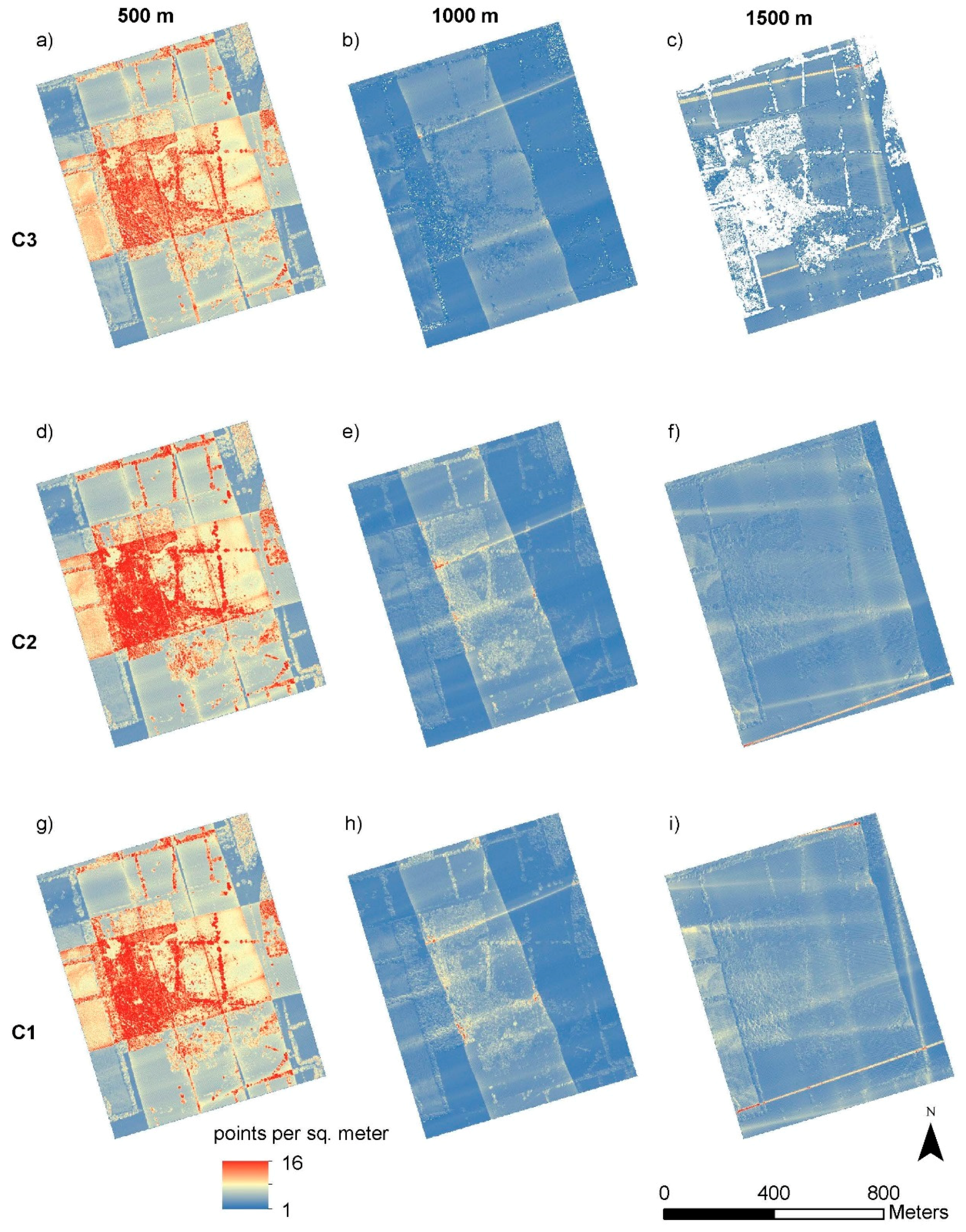
2.3.1. Point Density
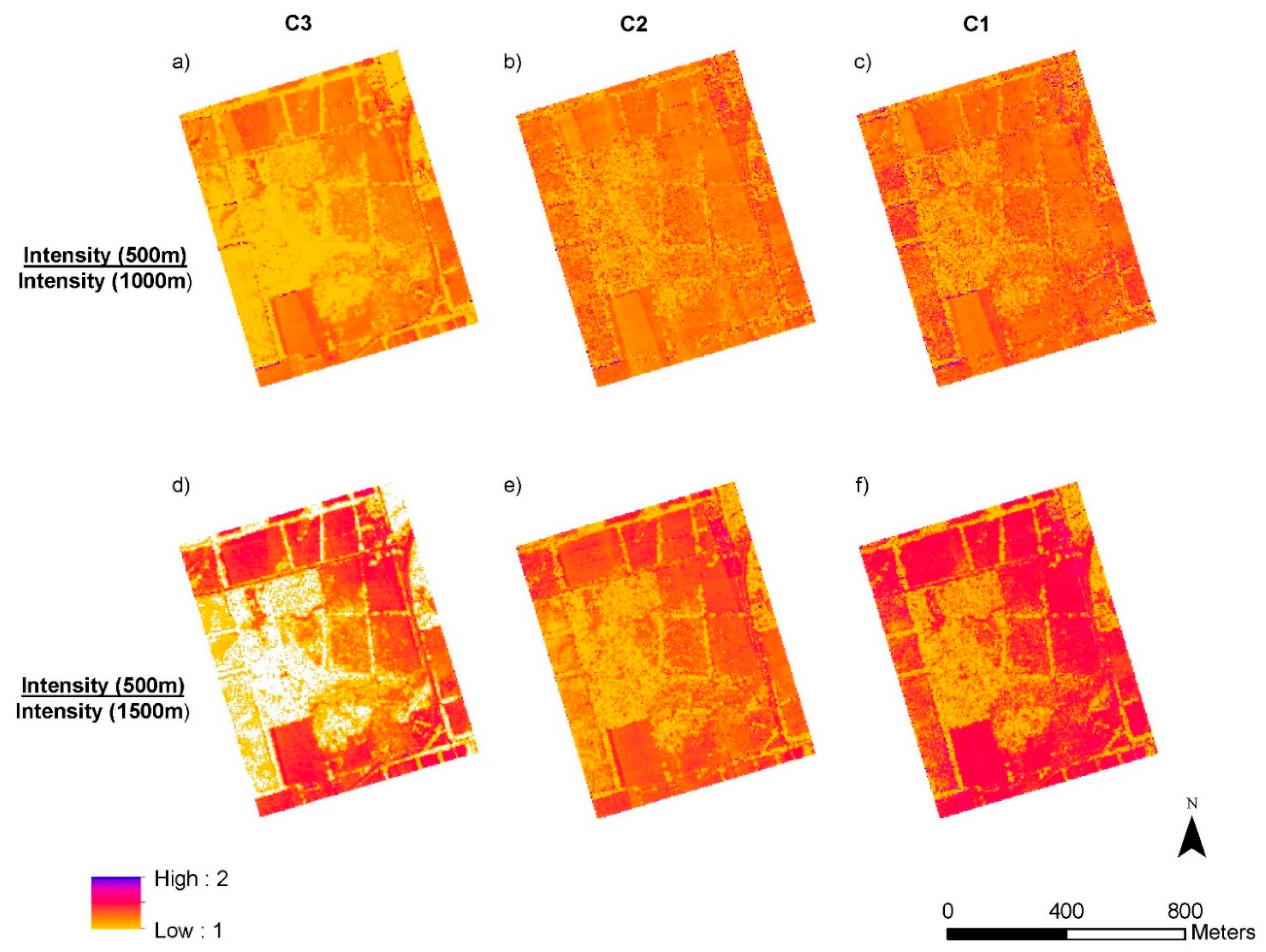
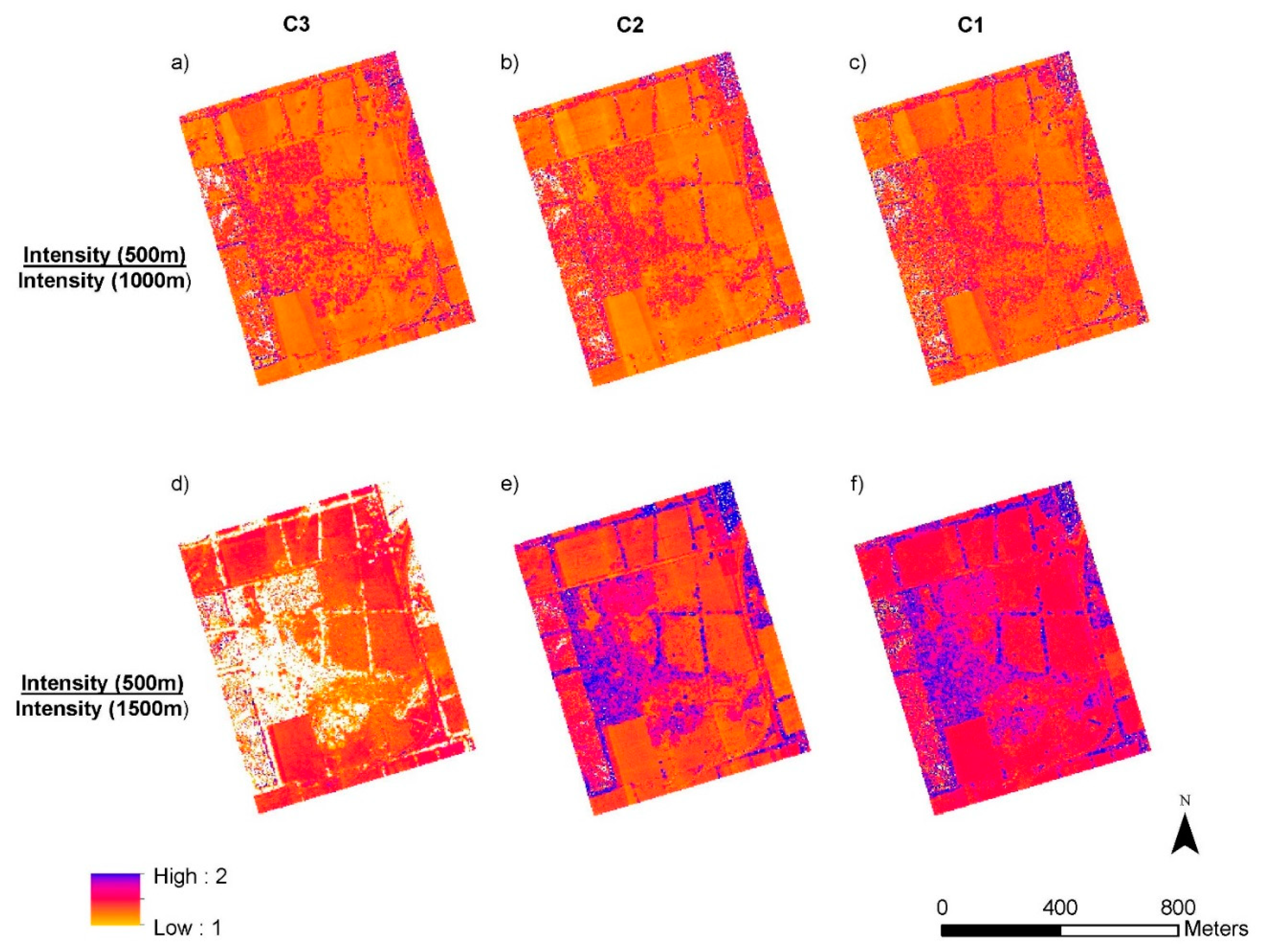
2.3.2. Single Channel Ratios
2.3.3. Spectral Vegetation Indices Maps
2.3.4. Spectral Vegetation Indices Ratios
3. Results
3.1. Point Density Maps
3.2. Single Channel Intensity Ratios
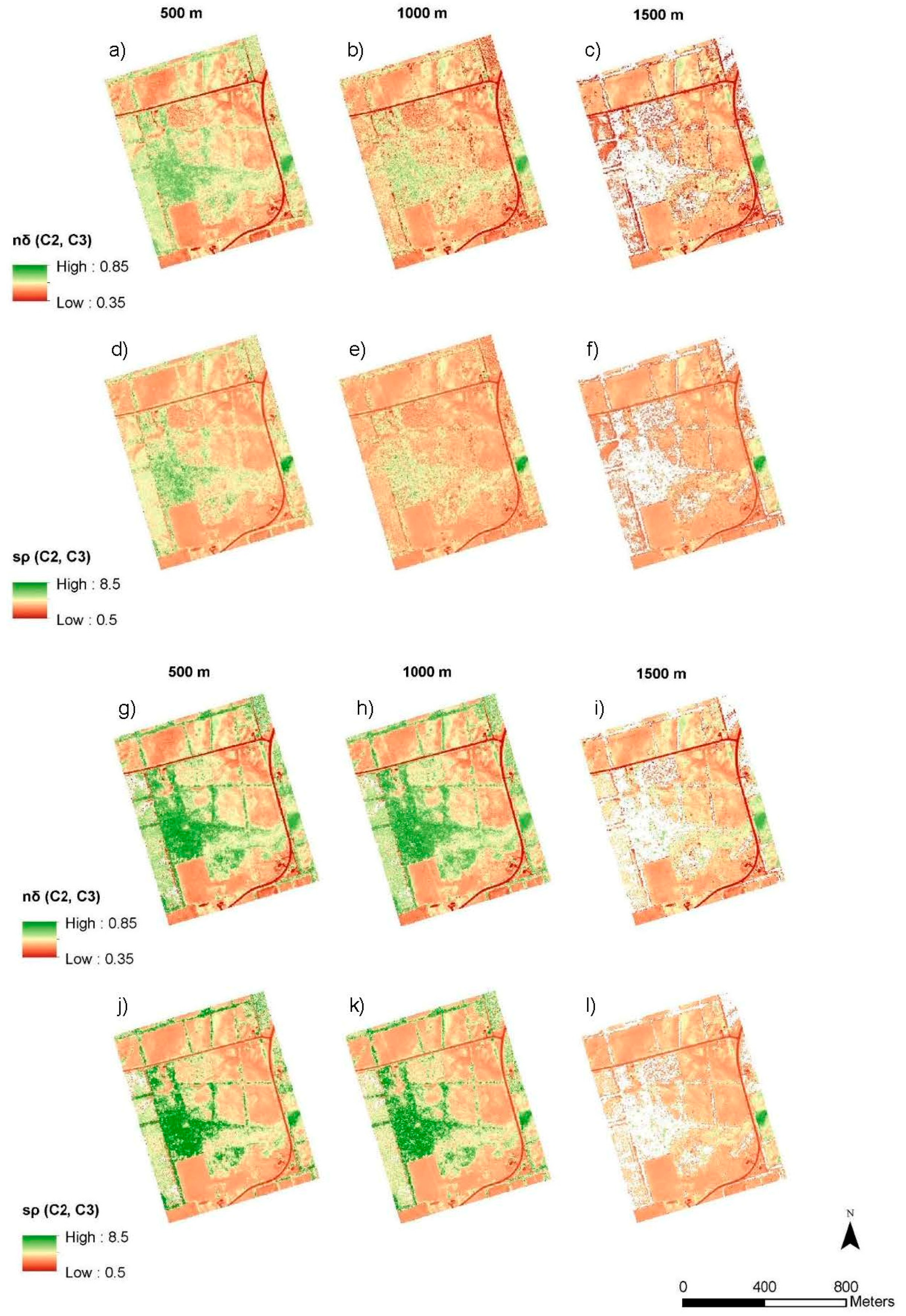
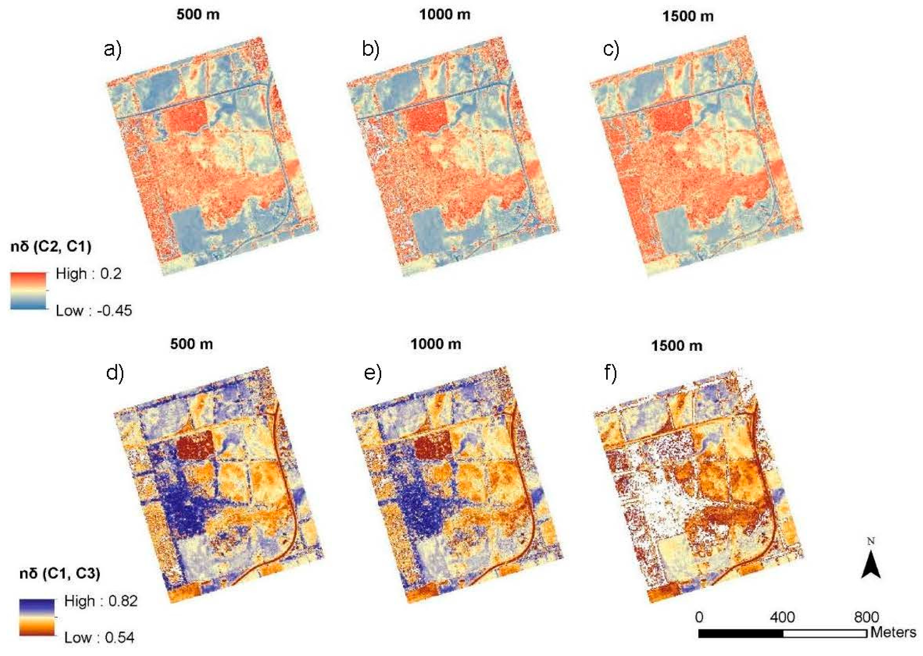
3.3. Spectral Vegetation Indices Maps
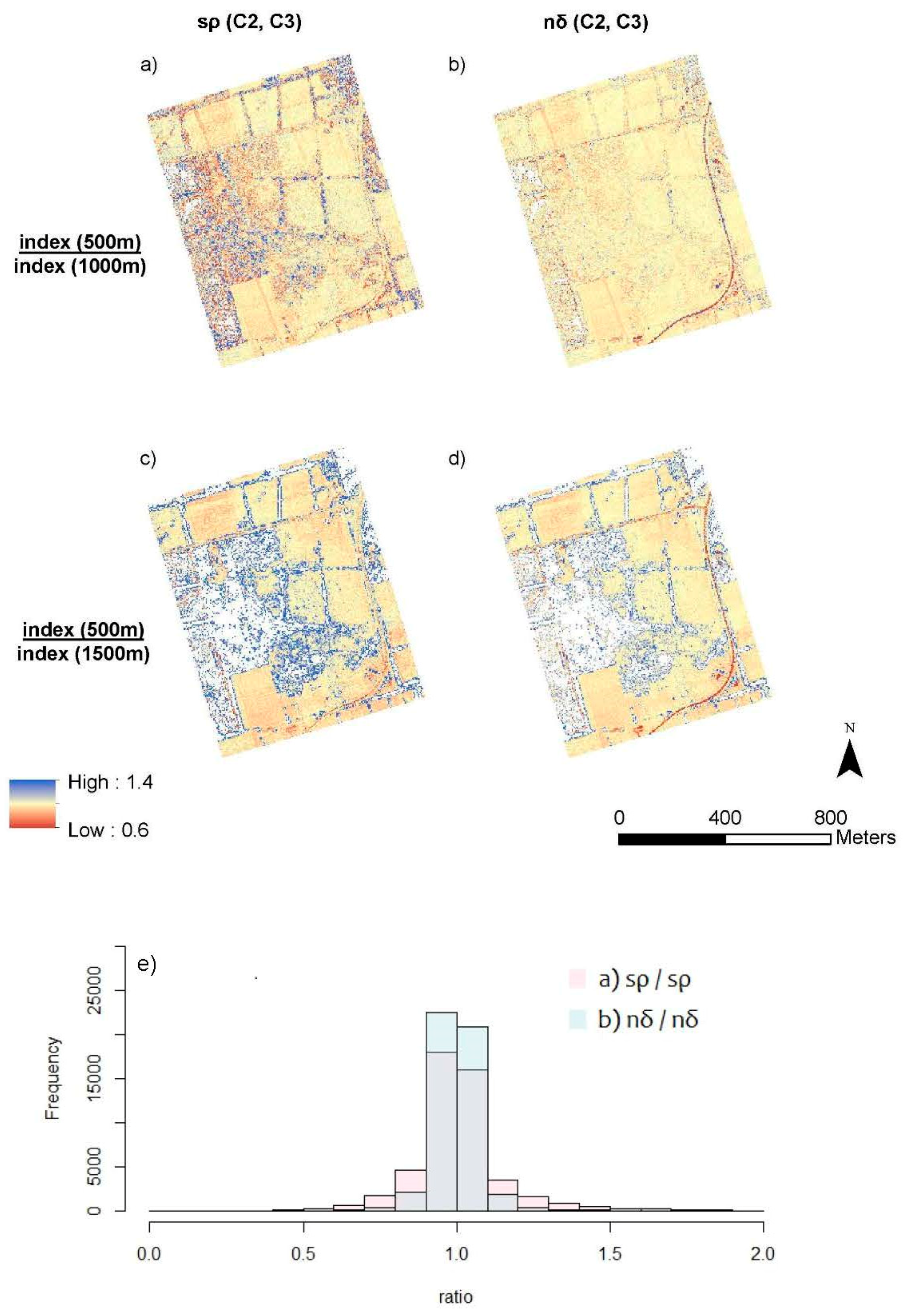
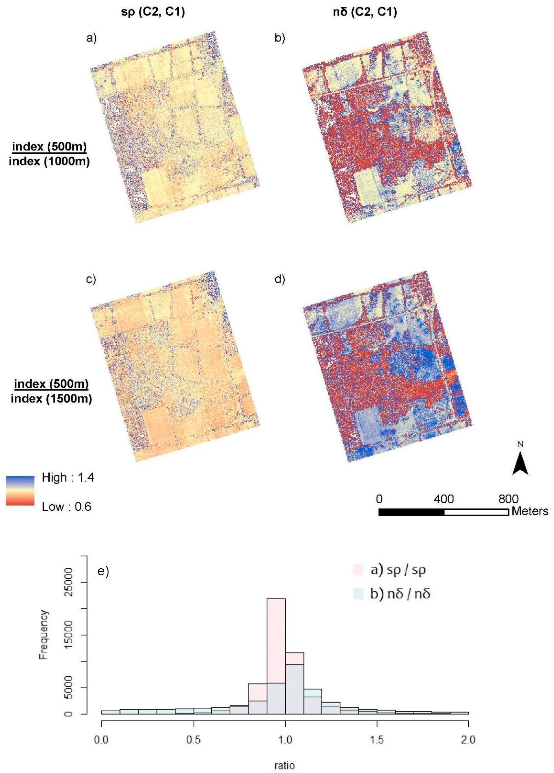
3.4. SVI Altitude Ratio Maps and Histograms
4. Discussion
5. Conclusions
Author Contributions
Funding
Acknowledgments
Conflicts of Interest
References
- Vosselman, G.; Maas, H. Airborne and Terrestrial Laser Scanning; CRC Press: Boca Raton, FL, USA, 2010. [Google Scholar]
- Lu, D.; Mausel, P.; Brondizio, E.; Moran, E. Change detection techniques. Int. J. Remote Sens. 2004, 25, 2365–2407. [Google Scholar] [CrossRef]
- Lyon, J.G.; Yuan, D.; Lunetta, R.S.; Elvidge, C.D. A change detection experiment using vegetation indices. Photogramm. Eng. Remote Sens. 1998, 64, 143–150. [Google Scholar]
- Pettorelli, N. The Normalized Difference Vegetation Index; Oxford University Press: Oxford, UK, 2013. [Google Scholar]
- Hopkinson, C.; Chasmer, L.; Gynan, C.; Mahoney, C.; Sitar, M. Multisensor and Multispectral LiDAR Characterization and Classification of a Forest Environment. Can. J. Remote. Sens. 2016, 42, 501–520. [Google Scholar] [CrossRef]
- Baret, F.; Guyot, G. Potentials and Limits of Vegetation Indexes for Lai and Apar Assessment. Remote Sens. Environ. 1991, 35, 161–173. [Google Scholar] [CrossRef]
- Huete, A.R. Soil and Sun angle interactions on partial canopy spectra. Int. J. Remote. Sens. 1987, 8, 1307–1317. [Google Scholar] [CrossRef]
- Jackson, R.D.; Slater, P.N.; Pinter, P.J. Discrimination of Growth and Water-Stress in Wheat by Various Vegetation Indexes through Clear and Turbid Atmospheres. Remote Sens. Environ. 1983, 13, 187–208. [Google Scholar] [CrossRef]
- Zhang, Y.; Chen, J.M.; Miller, J.R.; Noland, T.L. Leaf chlorophyll content retrieval from airborne hyperspectral remote sensing imagery. Remote Sens. Environ. 2008, 112, 3234–3247. [Google Scholar] [CrossRef]
- Gaulton, R.; Danson, F.; Ramírez, F.; Gunawan, O.; Danson, F. The potential of dual-wavelength laser scanning for estimating vegetation moisture content. Remote. Sens. Environ. 2013, 132, 32–39. [Google Scholar] [CrossRef]
- Morsdorf, F.; Nichol, C.; Malthus, T.; Woodhouse, I.H. Assessing forest structural and physiological information content of multi-spectral LiDAR waveforms by radiative transfer modelling. Remote. Sens. Environ. 2009, 113, 2152–2163. [Google Scholar] [CrossRef]
- Hakala, T.; Nevalainen, O.; Kaasalainen, S.; Mäkipää, R. Technical Note: Multispectral lidar time series of pine canopy chlorophyll content. Biogeosciences 2015, 12, 1629–1634. [Google Scholar] [CrossRef]
- Rees, W.G. Physical Principles of Remote Sensing, 2nd ed.; Cambridge University Press: Cambridge, UK, 2004. [Google Scholar]
- Perry, C.R.; Lautenschlager, L.F. Functional Equivalence of Spectral Vegetation Indexes. Remote Sens. Environ. 1984, 14, 169–182. [Google Scholar] [CrossRef]
- Rouse, J., Jr.; Haas, R.H.; Schell, J.A.; Deering, D.W. Monitoring Vegetation Systems in the Great Plains with ERTS; NASA Special Publication: Washington, DC, USA, 1974; p. 351. [Google Scholar]
- Fernandez-Diaz, J.C.; Carter, W.E.; Glennie, C.; Shrestha, R.L.; Pan, Z.; Ekhtari, N.; Singhania, A.; Hauser, D.; Sartori, M. Capability Assessment and Performance Metrics for the Titan Multispectral Mapping Lidar. Remote. Sens. 2016, 8, 936. [Google Scholar] [CrossRef]
- Gates, D.M.; Keegan, H.J.; Schleter, J.C.; Weidner, V.R. Spectral Properties of Plants. Appl. Opt. 1965, 4, 11–20. [Google Scholar] [CrossRef]
- Gamon, J.A.; Serrano, L.; Surfus, J.S. The photochemical reflectance index: An optical indicator of photosynthetic radiation use efficiency across species, functional types, and nutrient levels. Oecologia 1997, 112, 492–501. [Google Scholar] [CrossRef] [PubMed]
- Gamon, J.; Peñuelas, J.; Field, C. A narrow-waveband spectral index that tracks diurnal changes in photosynthetic efficiency. Remote. Sens. Environ. 1992, 41, 35–44. [Google Scholar] [CrossRef]
- Hardisky, M.A.; Klemas, V.; Smart, R.M. The Influence of Soil-Salinity, Growth Form, and Leaf Moisture on the Spectral Radiance of Spartina-Alterniflora Canopies. Photogramm. Eng. Remote Sens. 1983, 49, 77–83. [Google Scholar]
- Hunt, E.R.; Rock, B.N. Detection of Changes in Leaf Water-Content Using near-Infrared and Middle-Infrared Reflectances. Remote Sens. Environ. 1989, 30, 43–54. [Google Scholar]
- Hancock, S.; Gaulton, R.; Danson, F.M. Angular Reflectance of Leaves with a Dual-Wavelength Terrestrial Lidar and Its Implications for Leaf-Bark Separation and Leaf Moisture Estimation. IEEE Trans. Geosci. Remote. Sens. 2017, 55, 1–7. [Google Scholar] [CrossRef]
- Chasmer, L.E.; Hopkinson, C.D.; Petrone, R.M.; Sitar, M. Using Multitemporal and Multispectral Airborne Lidar to Assess Depth of Peat Loss and Correspondence with a New Active Normalized Burn Ratio for Wildfires. Geophys. Res. Lett. 2017, 44. [Google Scholar] [CrossRef]
- Xu, H.Q. Modification of normalised difference water index (NDWI) to enhance open water features in remotely sensed imagery. Int. J. Remote Sens. 2006, 27, 3025–3033. [Google Scholar] [CrossRef]
- Morsy, S.; Shaker, A.; El-Rabbany, A.; Larocque, P.E. Airborne multispectral lidar data for land-cover classification and land/water mapping using different spectral indexes. ISPRS Ann. Photogramm. Remote. Sens. Spat. Inf. Sci. 2016, 3, 217–224. [Google Scholar] [CrossRef]
- Schott, J.R. Remote Sensing: The Image Chain Approach, 2nd ed.; Oxford University Press: Oxford, UK, 2007. [Google Scholar]
- Jelalian, A. Laser Radar Systems; Artech House: Norwood, MA, USA, 1992. [Google Scholar]
- Wagner, W. Radiometric calibration of small-footprint full-waveform airborne laser scanner measurements: Basic physical concepts. ISPRS J. Photogramm. Remote. Sens. 2010, 65, 505–513. [Google Scholar] [CrossRef]
- Baltsavias, E. Airborne laser scanning: Basic relations and formulas. ISPRS J. Photogramm. Remote. Sens. 1999, 54, 199–214. [Google Scholar] [CrossRef]
- Hopkinson, C. The influence of flying altitude, beam divergence, and pulse repetition frequency on laser pulse return intensity and canopy frequency distribution. Can. J. Remote. Sens. 2007, 33, 312–324. [Google Scholar] [CrossRef]
- Yan, W.Y.; Shaker, A.; El-Ashmawy, N. Urban land cover classification using airborne LiDAR data: A review. Remote. Sens. Environ. 2015, 158, 295–310. [Google Scholar] [CrossRef]
- Korpela, I.; Tuomola, T.; Tokola, T.; Dahlin, B. Appraisal of seedling stand vegetation with airborne imagery and discrete-return LiDAR—An exploratory analysis. Silva Fenn. 2008, 42, 753–772. [Google Scholar] [CrossRef]
- Hopkinson, C.; Chasmer, L. Testing LiDAR models of fractional cover across multiple forest ecozones. Remote. Sens. Environ. 2009, 113, 275–288. [Google Scholar] [CrossRef]
- García, M.; Riaño, D.; Chuvieco, E.; Danson, F.M. Estimating biomass carbon stocks for a Mediterranean forest in central Spain using LiDAR height and intensity data. Remote. Sens. Envtron. 2010, 114, 816–830. [Google Scholar] [CrossRef]
- Holmgren, J.; Persson, Å. Identifying species of individual trees using airborne laser scanner. Remote. Sens. Environ. 2004, 90, 415–423. [Google Scholar] [CrossRef]
- Donoghue, D.N.; Watt, P.J.; Cox, N.J.; Wilson, J. Remote sensing of species mixtures in conifer plantations using LiDAR height and intensity data. Remote. Sens. Environ. 2007, 110, 509–522. [Google Scholar] [CrossRef]
- Korpela, I.; Ørka, H.; Maltamo, M.; Tokola, T.; Hyyppä, J. Tree species classification using airborne LiDAR—Effects of stand and tree parameters, downsizing of training set, intensity normalization, and sensor type. Silva Fenn. 2010, 44, 319–339. [Google Scholar] [CrossRef]
- Yan, W.Y.; Shaker, A.; Habib, A.; Kersting, A.P. Improving classification accuracy of airborne LiDAR intensity data by geometric calibration and radiometric correction. ISPRS J. Photogramm. Remote. Sens. 2012, 67, 35–44. [Google Scholar] [CrossRef]
- Roncat, A.; Morsdorf, F.; Briese, C.; Wagner, W.; Pfeifer, N. Laser Pulse Interaction with Forest Canopy: Geometric and Radiometric Issues. For. Appl. Airborne Laser Scanning: Concepts Case Stud. 2014, 27, 19–41. [Google Scholar]
- Wagner, W.; Ullrich, A.; Ducic, V.; Melzer, T.; Studnicka, N. Gaussian decomposition and calibration of a novel small-footprint full-waveform digitising airborne laser scanner. ISPRS J. Photogramm. Remote. Sens. 2006, 60, 100–112. [Google Scholar] [CrossRef]
- Nicodemus, F.E.; Richmond, J.C.; Hsia, J.J.; Ginsberg, I.W.; Limperis, T. Geometrical Considerations and Nomenclature for Reflectance; US Department of Commerce, National Bureau of Standards: Washington, DC, USA, 1977.
- Kukko, A.; Kaasalainen, S.; Litkey, P. Effect of incidence angle on laser scanner intensity and surface data. Appl. Opt. 2008, 47, 986. [Google Scholar] [CrossRef]
- Govaerts, Y.M.; Jacquemoud, S.; Verstraete, M.M.; Ustin, S.L. Three-dimensional radiation transfer modeling in a dicotyledon leaf. Appl. Opt. 1996, 35, 6585. [Google Scholar] [CrossRef] [PubMed]
- Li, Z.; Jupp, D.L.B.; Strahler, A.H.; Schaaf, C.B.; Howe, G.; Hewawasam, K.; Douglas, E.S.; Chakrabarti, S.; Cook, T.A.; Paynter, I.; et al. Radiometric Calibration of a Dual-Wavelength, Full-Waveform Terrestrial Lidar. Sensors 2016, 16, 313. [Google Scholar] [CrossRef]
- Kaasalainen, S.; Hyyppa, H.; Kukko, A.; Litkey, P.; Ahokas, E.; Hyyppa, J.; Lehner, H.; Jaakkola, A.; Suomalainen, J.; Akujarvi, A.; et al. Radiometric Calibration of LIDAR Intensity with Commercially Available Reference Targets. IEEE Trans. Geosci. Remote. Sens. 2009, 47, 588–598. [Google Scholar] [CrossRef]
- Okhrimenko, M.; Coburn, C.; Hopkinson, C. Investigating Multi-Spectral Lidar Radiometry: An Overview of the Experimental Framework. In Proceedings of the IGARSS 2018—2018 IEEE International Geoscience and Remote Sensing Symposium, Valencia, Spain, 23–27 July 2018; pp. 8745–8748. [Google Scholar]
- Okhrimenko, M.; Hopkinson, C. Multi-spectral lidar: Radiometric calibration, canopy reflectance, and vegetation vertical SVI profiles. Remote Sens. 2019, submitted. [Google Scholar]
- Steven, M.D.; Malthus, T.J.; Baret, F.; Xu, H.; Chopping, M.J. Intercalibration of vegetation indices from different sensor systems. Remote. Sens. Environ 2003, 88, 412–422. [Google Scholar] [CrossRef]
- Yan, W.Y.; Shaker, A. Airborne LiDAR intensity banding: Cause and solution. ISPRS J. Photogramm. Remote. Sens. 2018, 142, 301–310. [Google Scholar] [CrossRef]
- Isenburg, M. LAStools—Efficient LiDAR Processing Software. (Version 161029, Academic). 2016. Available online: http://rapidlasso.com/LAStools (accessed on 15 August 2016).
- Lin, M.F.; Lucas, H.C.; Shmueli, G. Too Big to Fail: Large Samples and the p-Value Problem. Inf. Syst. Res. 2013, 24, 906–917. [Google Scholar] [CrossRef]
- Budei, B.C.; St-Onge, B.; Hopkinson, C.; Audet, F.-A. Identifying the genus or species of individual trees using a three-wavelength airborne lidar system. Remote. Sens. Environ. 2018, 204, 632–647. [Google Scholar] [CrossRef]
- Morsy, S.; Shaker, A.; El-Rabbany, A.; Passaro, V.M.N. Multispectral LiDAR Data for Land Cover Classification of Urban Areas. Sensors 2017, 17, 958. [Google Scholar] [CrossRef] [PubMed]


| Flight Line (L) | L1 | L2 | L3 | L4 | L5 | L6 | L7 | L8 | L9 | L10 |
|---|---|---|---|---|---|---|---|---|---|---|
| <Range>, m | 491 | 540 | 547 | 546 | 536 | 942 | 1018 | 1475 | 1540 | 1555 |
| PRF*, kHz | 75 | 75 | 75 | 75 | 75 | 75 | 75 | 75 | 75 | 75 |
| SF, Hz | 40 | 40 | 40 | 40 | 40 | 38 | 38 | 32 | 32 | 32 |
| Swath, deg | 40.0 | 40.0 | 40.0 | 40.0 | 40.0 | 40.0 | 40.0 | 40.0 | 40.0 | 40.0 |
| <Speed>, m/s | 67 | 65 | 65 | 69 | 66 | 63 | 68 | 64 | 59 | 68 |
| Heading, deg | 160 | 340 | 160 | 340 | 250 | 160 | 340 | 160 | 340 | 250 |
| 500 m | 1000 m | 1500 m | |||||||
|---|---|---|---|---|---|---|---|---|---|
| C1/C2/C3 | C1 | C2 | C3 | C1 | C2 | C3 | C1 | C2 | C3 |
| Wavelength | 1550 nm | 1064 nm | 532 nm | 1550 nm | 1064 nm | 532 nm | 1550 nm | 1064 nm | 532 nm |
| Point density all | 8.05 | 8.35 | 7.57 | 2.55 | 2.57 | 1.9 | 3.14 | 2.85 | 2.38 |
| Point density last | 5.7 | 5.71 | 5.68 | 2 | 2 | 1.8 | 2.8 | 2.59 | 2.38 |
| Spacing all, cm | 0.35 | 0.35 | 0.36 | 0.63 | 0.62 | 0.73 | 0.56 | 0.59 | 0.65 |
| Number of returns | 6,468,902 | 6,709,651 | 6,083,545 | 2,050,152 | 2,059,638 | 1,502,604 | 2,525,347 | 2,291,578 | 1,337,302 |
| Footprint diameter at nadir, cm | 18 | 18 | 35 | 35 | 35 | 70 | 53 | 53 | 105 |
| Single | 3,269,931 | 3,151,688 | 3,344,283 | 1,236,739 | 1,231,412 | 1,347,771 | 1,984,104 | 1,887,007 | 1,336,696 |
| Double | 1,741,204 | 1,822,086 | 1,903,834 | 591,220 | 606,513 | 153,513 | 518,169 | 368,437 | 606 |
| Triple | 933,480 | 1,087,821 | 673,996 | 181,753 | 183,627 | 1,316 | 22,510 | 35,130 | 0 |
| Quadruple | 524,287 | 648,056 | 161,432 | 40,440 | 38,086 | 4 | 564 | 1,004 | 0 |
| First | 4,584,010 | 4,588,576 | 4,562,217 | 1,603,452 | 1,605,753 | 1,425,026 | 2,251,163 | 2,083,401 | 1,336,999 |
| Second | 1,312,320 | 1,435,277 | 1,216,281 | 366,052 | 373,756 | 77,137 | 266,407 | 195,979 | 303 |
| Third | 441,804 | 524,168 | 264,788 | 70,566 | 70,627 | 440 | 7,636 | 11,947 | 0 |
| Fourth | 130,768 | 161,630 | 40,259 | 10082 | 9502 | 1 | 141 | 251 | 0 |
| 500 m | 1000 m | 1500 m | |||||||
|---|---|---|---|---|---|---|---|---|---|
| C1/C2/C3 Wavelength, nm | C1 1550 | C2 1054 | C3 532 | C1 1550 | C2 1064 | C3 532 | C1 1550 | C2 1064 | C3 532 |
| Hay stubble | 5.3 | 5.35 | 5.0 | 2.5 | 2.4 | 2.0 | 3.2 | 2.9 | 2.6 |
| Coniferous all | 9.9 | 10.8 | 9.7 | 4.0 | 3.6 | 2.6 | 2.6 | 2.2 | 0.1 |
| Coniferous single | 3.4 | 2.7 | 3.6 | 2.0 | 1.5 | 2.1 | 2.2 | 1.5 | 0.1 |
| Deciduous all | 14.3 | 15.1 | 12.0 | 3.3 | 3.3 | 1.3 | 3.4 | 2.7 | <0.1 |
| Deciduous single | 2.3 | 1.9 | 3.2 | 0.9 | 0.9 | 1.1 | 2.0 | 1.6 | <0.1 |
| Mixed all | 12.7 | 14.0 | 11.4 | 3.7 | 3.8 | 1.8 | 3.0 | 2.6 | 0.1 |
| Mixed singles | 3.1 | 2.6 | 3.5 | 1.4 | 1.3 | 1.6 | 2.1 | 1.7 | 0.1 |
| Crop all | 5.0 | 5.2 | 5.1 | 1.3 | 1.6 | 1.3 | 2.7 | 2.3 | 0.2 |
| Crop singles | 1.1 | 1.0 | 0.8 | 0.4 | 0.6 | 0.8 | 1.1 | 1.5 | 0.2 |
| Range, m | C1 (1550 nm) | C2 (1064 nm) | C3 (532 nm) | |||||||
|---|---|---|---|---|---|---|---|---|---|---|
| N | N | N | ||||||||
| L3 | 515 | 580 | 772.2 (51.9) | 778,0 (54.0) | 486 | 394.0 (30.5) | 396.5 (30.7) | 556 | 136.6 (11.0) | 137.5 (11.1) |
| KS test | D = 0.133 p < 0.01 | D = 0.095 p = 0.012 | D = 0.132 p < 0.01 | D = 0.094 p = 0.018 | D = 0.038 p = 0.997 | D = 0.205 p < 0.01 | ||||
| L4 | 525 | 536 | 759.6 (52.7) | 790.2 (54.7) | 591 | 383.9 (28.6) | 389.4 (29.0) | 418 | 137.1 (10.8) | 142.3 (11.2) |
| L3/L4 | 1.07 | 0.98 | 1.03 | 1.02 | 1.00 | 1.00 | ||||
| L6 | 916 | 280 | 643.7 (41.6) | 646.8 (41.8) | 294 | 328.6 (22.7) | 330.2 (22.8) | 289 | 114.6 (8.2) | 115.0 (8.3) |
| KS test | D = 0.688 p < 0.01 | D = 0.544 p < 0.01 | D = 0.436 p < 0.01 | D = 0261 p < 0.01 | D = 0.630 p < 0.01 | D = 0.461 p < 0.01 | ||||
| L7 | 1023 | 253 | 571.3 (36.8) | 595.5 (38.0) | 266 | 304.6 (19.0) | 317.6 (19.8) | 290 | 102.3 (6.7) | 106.7 (7.0) |
| L6/L7 | 1.13 | 1.09 | 1.08 | 1.04 | 1.12 | 1.08 | ||||
| (L3+L4)/(L6+L7) | 1.26 | 1.26 | 1.23 | 1.21 | 1.26 | 1.26 | ||||
| L8 | 1460 | 250 | 553.4 (30.8) | 553.4 (30.8) | 218 | 301.5 (16.7) | 301.5 (16.7) | 881 | 100.8 (7.4) | 100.8 (7.4) |
| KS test | D = 0.506 p < 0.01 | D = 0.425 p < 0.01 | D = 0.330 p < 0.01 | D = 0.220 p < 0.01 | D = 0.233 p < 0.01 | D = 0.184 p < 0.01 | ||||
| L9 | 1514 | 212 | 514.1 (29.6) | 522.6(30.1) | 198 | 289.4 (16.7) | 294.3 (17.0) | 190 | 97.0 (7.1) | 98.7 (7.2) |
| L8/L9 | 1.08 | 1.06 | 1.04 | 1.02 | 1.04 | 1.02 | ||||
| (L3+L4)/(L8+L9) | 1.43 | 1.46 | 1.32 | 1.32 | 1.38 | 1.40 | ||||
| All Returns | Paired Test, p-Value | Single Returns | ||||||
|---|---|---|---|---|---|---|---|---|
| MEAN | SD | p | MEAN | SD | p | |||
| a) | C3(500 m)/C3(1000 m) | 1.08 | 0.20 | <0.01 | <0.01 | 1.31 | 0.23 | <0.01 |
| d) | C3(500 m)/C3(1500 m) | 1.14 | 0.30 | <0.01 | <0.01 | 1.30 | 0.18 | <0.01 |
| b) | C2(500 m)/C2(1000 m) | 1.19 | 0.15 | <0.01 | <0.01 | 1.31 | 0.23 | <0.01 |
| e) | C2(500 m)/C2(1500 m) | 1.20 | 0.17 | <0.01 | <0.01 | 1.51 | 0.33 | <0.01 |
| c) | C1(500 m)/C1(1000 m) | 1.22 | 0.20 | <0.01 | <0.01 | 1.34 | 0.27 | <0.01 |
| f) | C1(500 m)/C1(1500 m) | 1.29 | 0.20 | <0.01 | <0.01 | 1.60 | 0.33 | <0.01 |
| Index | AGL, m | (C2,C3) | (C2,C1) | (C1,C3) | |||
|---|---|---|---|---|---|---|---|
| (1064 nm, 532 nm) | (1064 nm, 1550 nm) | (1550 nm, 532 nm) | |||||
| <all> | <single> | <all> | <single> | <all> | <single> | ||
| nδ | 500 | 0.57 (0.10) | 0.60 (0.12) | −0.14 (0.13) | −0.12 (0.16) | 0.66 (0.06) | 0.68 (0.07) |
| 1000 | 0.54 (0.09) D = 0.19, p < 0.01 | 0.60 (0.12) D = 0.02, p < 0.01 | −0.13 (0.14) D = 0.05, p < 0.01 | −0.11 (0.16) D = 0.03, p < 0.01 | 0.62 (0.08) D = 0.24, p < 0.01 | 0.67 (0.07) D = 0.03, p < 0.01 | |
| 1500 | 0.50 (0.09) D = 0.33, p < 0.01 | 0.54 (0.08) D = 0.31, p < 0.01 | −0.11 (0.13) D = 0.10, p < 0.01 | −0.09 (0.14) D = 0.11, p < 0.01 | 0.60 (0.10) D = 0.31, p < 0.01 | 0.62 (0.08) D = 0.26, p < 0.01 | |
| sρ | 500 | 3.91 (1.11) | 4.54 (2.03) | 0.78 (0.23) | 0.82 (0.27) | 5.12 (1.05) | 5.53 (1.60) |
| 1000 | 3.47 (0.85) D = 0.19, p < 0.01 | 4.49 (1.85) D = 0.02, p < 0.01 | 0.80 (0.23) D = 0.05, p < 0.01 | 0.84 (0.28) D = 0.03, p < 0.01 | 4.51 (1.09) D = 0.24, p < 0.01 | 5.42 (1.55) D = 0.03, p < 0.01 | |
| 1500 | 3.16 (0.75) D = 0.33, p < 0.01 | 3.44 (0.73) D = 0.31, p < 0.01 | 0.83 (0.21) D = 0.10, p < 0.01 | 0.87 (0.24) D = 0.11, p < 0.01 | 4.24 (1.17) D = 0.31, p < 0.01 | 4.49 (1.04) D = 0.26, p < 0.01 | |
| 500 m/1000 m | 500 m/1500 m | ||||||
|---|---|---|---|---|---|---|---|
| Mean(SD) | min | max | Mean(SD) | min | max | ||
| (C2,C3) | sρ | 1.02(0.20) | 0.15 | 10.10 | 1.13(0.40) | 0.29 | 11.13 |
| nδ | 1.00(0.62) | −11.95 | 130.06 | 1.05(0.33) | −35.06 | 28.14 | |
| (C2,C1) | sρ | 1.00(0.18) | 0.08 | 6.09 | 0.96(0.16) | 0.07 | 5.78 |
| nδ | 0.80(3.83) | −103.06 | 118.32 | 0.95(4.14) | −126.80 | 123.60 | |
| (C1,C3) | sρ | 1.03(0.21) | 0.08 | 12.68 | 1.21(0.41) | 0.16 | 12.30 |
| nδ | 1.01(0.09) | −5.92 | 8.43 | 1.09(0.22) | −15.81 | 12.07 | |
| 532 nm | 1064 nm | 1550 nm | |
| 500 m | ~ 4.2/2.4 | ~ 4.5/2.5 | ~4.2/2.4 |
| 1000 m | ~ 1.0 /1.3 | ~2.0/1.3 | ~ 2.1/1.3 |
| 1500 m | ~ 0.04/0.8 | ~0.8/0.8 | ~ 0.9/0.9 |
© 2019 by the authors. Licensee MDPI, Basel, Switzerland. This article is an open access article distributed under the terms and conditions of the Creative Commons Attribution (CC BY) license (http://creativecommons.org/licenses/by/4.0/).
Share and Cite
Okhrimenko, M.; Hopkinson, C. Investigating the Consistency of Uncalibrated Multispectral Lidar Vegetation Indices at Different Altitudes. Remote Sens. 2019, 11, 1531. https://doi.org/10.3390/rs11131531
Okhrimenko M, Hopkinson C. Investigating the Consistency of Uncalibrated Multispectral Lidar Vegetation Indices at Different Altitudes. Remote Sensing. 2019; 11(13):1531. https://doi.org/10.3390/rs11131531
Chicago/Turabian StyleOkhrimenko, Maxim, and Chris Hopkinson. 2019. "Investigating the Consistency of Uncalibrated Multispectral Lidar Vegetation Indices at Different Altitudes" Remote Sensing 11, no. 13: 1531. https://doi.org/10.3390/rs11131531
APA StyleOkhrimenko, M., & Hopkinson, C. (2019). Investigating the Consistency of Uncalibrated Multispectral Lidar Vegetation Indices at Different Altitudes. Remote Sensing, 11(13), 1531. https://doi.org/10.3390/rs11131531