Ship Detection from Optical Remote Sensing Images Using Multi-Scale Analysis and Fourier HOG Descriptor

Abstract

Automatic ship detection by Unmanned Airborne Vehicles (UAVs) and satellites is one of the fundamental challenges in maritime research due to the variable appearances of ships and complex sea backgrounds. To address this issue, in this paper, a novel multi-level ship detection algorithm is proposed to detect various types of offshore ships more precisely and quickly under all possible imaging variations. Our object detection system consists of two phases. First, in the category-independent region proposal phase, the steerable pyramid for multi-scale analysis is performed to generate a set of saliency maps in which the candidate region pixels are assigned to high salient values. Then, the set of saliency maps is used for constructing the graph-based segmentation, which can produce more accurate candidate regions compared with the threshold segmentation. More importantly, the proposed algorithm can produce a rather smaller set of candidates in comparison with the classical sliding window object detection paradigm or the other region proposal algorithms. Second, in the target identification phase, a rotation-invariant descriptor, which combines the histogram of oriented gradients (HOG) cells and the Fourier basis together, is investigated to distinguish between ships and non-ships. Meanwhile, the main direction of the ship can also be estimated in this phase. The overall algorithm can account for large variations in scale and rotation. Experiments on optical remote sensing (ORS) images demonstrate the effectiveness and robustness of our detection system.

1. Introduction

With the rapid development of the Earth Observing Satellite Technique, more high-resolution optical remote sensing (ORS) data become available, which enlarges the potential of ORS data for image analysis. Automatic ship detection is of great importance to military and civilian applications. This is a challenging task in the field of ORS image processing due to the variable appearances of ships and complex sea backgrounds. More specifically, ship targets in ORS images can vary greatly in illumination, color, texture, and other visual properties. Due to the overhead view, they are relatively small in size. Meanwhile, they often appear in very different scales and directions. Besides, ships are easily confused with the interferences introduced by heavy clouds, islands, coastlines, ocean waves, and other uncertain sea state conditions, which further increases the difficulty of ship detection. Therefore, how to detect various types of ships quickly and precisely from ORS images with cluttered scenes has become an urgent problem to be solved.

According to the geographical location of ship targets, existing detection algorithms fall into two categories, inshore ship detection and offshore ship detection. Note that land areas can be eliminated by using sea-land segmentation or prior geographic information, for instance, a Geographic Information System (GIS) database. We consider the problem of detecting and localizing offshore ships in ORS images in this paper. Over the last decades, numerous ship detection algorithms have been investigated. Most current existing methods adopt a two-stage detection mechanism, namely, region proposal and ship target identification. The goal of the region proposal stage is to separate regions of interest (ROIs) from the background for the subsequent target identification. The first type of methods used the threshold segmentation techniques [1,2], which set an optimal threshold and regarded pixels with gray value beyond the threshold as the target pixels. Zhu et al. [1] applied the Otsu segmentation followed by a level set to extract candidate regions. Leng et al. [2] employed the same segmentation algorithm to distinguish potential target and clutter pixels. These methods have a small computational effort and work well on the simple ocean scenes. Nevertheless, they perform poorly when the target’s intensity is similar to or even lower than the clutter. Besides, massive clouds are easily mistaken for targets because they are usually brighter than the background. This would generate plenty of false alarms in the candidate extraction stage. The second type of methods performed the sliding window where every location within the target image was examined in order not to miss any potential target location. For instance, Zhou et al. [3] used the multi-scale sliding window to obtain patches from the test images and employed the sparse code and support vector machine (SVM) classification in the ship validation stage. However, the exhaustive search has several drawbacks. First, lack of prior information of target size, the multiple scales, and multiple aspect ratios are needed to guarantee the detection accuracy. The number of windows to visiting remains huge. On the other hand, the captured ship targets only take up a few pixels in large sea images, that is to say, only a few windows contain real ship targets. It is inappropriate for remote sensing images to use sliding window detection mechanism, which is time-consuming and computationally complex. Since the ships in the visible remote sensing (VRS) image of the sea are salient objects, they are usually sparsely distributed and can easily be identified by the human visual attention system. Recently, the saliency model, which can extract ROIs efficiently, has become a hot spot in ORS image processing. There is a significant body of work on the saliency model, including several kinds of spatial-domain models and a variety of transform-domain models. One of the classical spatial-domain models is the one proposed by Itti et al. in 1998 [4]. This model extracted simple visual features, including color, intensity, and orientation, by the center-surround strategy. Then, the conspicuity maps of each feature were obtained by performing the across-scale combination. The final saliency map was generated by fusing these conspicuity maps. Subsequently, a large number of models have been proposed to predict salient pixels. We refer readers to [5] for more details. The transform-domain saliency model, which requires a small amount of computation, plays an important role in ship detection. Zhuang et al. [6] came up with an extended version of the spectral residual model to rapidly complete ship candidate extraction. Zhang et al. [7] extracted the ROIs in HSI color space based on quaternion Fourier transform. In addition, Xu et al. [8] designed another saliency model based on wavelet transform for obtaining the ship targets. The saliency models mentioned above can quickly remove redundant information and restrain the complex and various backgrounds. They achieve considerable detection results even in the presence of cloud, fog, sea clutter, etc. However, the existing salient-region based methods are sensitive to the variety of target size. They are not suitable for dealing with situations where ship targets have a large difference in size. Moreover, there is usually a threshold segmentation step to segment saliency map and obtain the binary image, which can distinguish the target from the sea background. This, however, is not wise because there may not be any ROI present in the target image. In summary, a practical region proposal algorithm should be robust to the variety of target size. Of equal importance, it should detect the targets accurately and suppress false alarms under complex backgrounds. Based on the challenges mentioned above, there still remains room for improvement in saliency detection from ORS images.

The aim of the ship discrimination stage is to distinguish between the real ships and the false alarms. The discrimination stage commonly contains two stages: feature extraction and classification. Powerful feature extraction is a very important part of constructing a high-performance object detector. Since the target orientation in ORS images is arbitrary, rotation-invariant object detection is of vital significance. Some traditional image features like the histogram of oriented gradients (HOG) feature [9] and the Haar feature [10] can achieve excellent detection precision and computation speed. Despite the popularity of these feature representation methods, they are not rotation-invariant due to the definition according to a fixed coordinate system. Great efforts have been made for solving this issue. Method [11] extracted an extra feature provided with HOG feature and generated four AdaBoost classifiers to detect ships in different orientations. In a similar manner, the method [12] divided ships into eight subsets according to their orientations and trained eight filters using linear SVM for classification, respectively. Yao et al. [10] used the Haar feature combined with three AdaBoost classifiers, which are trained for three directions using samples with different directions. Because of the need to train multiple classifiers, which have complex training steps and great computational cost, these methods are not suitable for real-time processing. Another type of method aligned the candidate regions with an estimated dominant orientation. Shi et al. [13] adopted a radon transform method to rotate the patches in order to make all the candidates distributed in the same direction. Qi et al. [14] performed the Principal Component Analysis (PCA) transform to obtain the direction of the main axis and rotated the ship candidates to the vertical direction before extracting HOG feature from the ship candidates. Method [15] obtained the main direction of ships by computing the HOG feature and rotated the ships in the same direction. By pre-rotating the patches to a fixed angle, the subsequent feature extraction does not need to take into account the target rotation problem. However, such methods are obviously sensitive to the incorrect estimates of dominant orientation. Instead of rotation estimation computation, a more elegant line of work focused on the rotation-invariant feature analysis for ship target description. Method [16] proposed a rotation-invariant matrix for object detection in ORS images. The proposed matrix could incorporate partial angular spatial information in addition to radial spatial information. Method [17] extracted a rotation-invariant feature describing the shape and the texture information of the targets. Then, a trainable SVM classifier was performed to further remove the false alarms and maintain the real ship targets. In general, the performances of these rotation-invariant features are satisfying in ship target description. After the feature extraction stage, a classifier outputs the predicted label of each candidate, i.e., object or not. Some methods used unsupervised learning in the identification stage. For example, the method [8] designed an unsupervised multi-level discrimination algorithm based on the improved entropy and pixel distribution to further reduce the false alarms. Method [18] applied efficient rules based on a novel gradient descriptor to distinguish ships and non-ships. Other methods applied the supervised learning to detect the ship targets, generally using SVM, AdaBoost, etc. Compared with unsupervised learning, these methods are more accurate and more suitable for ship target detection. To sum up, a good ship identification algorithm should not only be highly discriminative to distinguish the ship targets and the false alarms but also be robust to the variable appearances of ships, such as rotation, illumination, scale, and viewpoint changes.

In recent years, a deep learning algorithm has become a powerful tool for remote sensing image analysis. It was initially attempted to represent features in the feature extraction stage. Yang et al. [12] implemented a deep forest ensemble with a cascade structure to discriminate ship targets. Wu et al. [19] presented a ship head feature extraction algorithm based on convolutional neural network (CNN). Method [20] combined the constant false alarm rate (CFAR) detection algorithm with the CNN model to detect ships in Synthetic aperture radar (SAR) images. Method [21] achieved rotation invariance by introducing and learning a new rotation-invariant layer on the basis of the existing CNN architecture. Method [22] presented an architecture, which used CNN for extracting features of aerial imagery, and applied a k-Nearest Neighbor method to examine if an aerial image of the visible spectrum contained a ship or not. Due to the strong feature representation power, deep learning algorithms achieved more discriminative data representation compared with hand-engineered features. With the development of deep learning algorithms, the end-to-end data-driven detectors, which consist of a region proposal network (RPN) and an object detection network, have been specially modified to detect the objects in the large remote sensing images. Some end-to-end detection models aim to overcome the problem of the large scale variability. Zhang et al. [23] proposed a multi-scale Feature Pyramid Network containing a multi-scale potential region generation and a multi-scale object detection network to detect small and dense objects. Li et al. [24] proposed a modification of faster region-CNN (Faster-RCNN) [25] by constructing a hierarchical selective filtering layer to accurately detect multi-scale ships. Other end-to-end detection models have been extended to overcome the issue of target rotation. For instance, Liu et al. [26] designed an arbitrary-oriented ship detection framework based on the YOLOv2 architecture [27] by adding the orientation loss to the loss function. These models utilized the unified detection framework instead of the multi-stage pipelines and achieved significant improvements in the ship detection task. However, such deep learning methods need a lot of training data as well as complex training phases. Their implementations rely on Graphical Processing Unit (GPU) and parallel operations. For small platforms like Unmanned Airborne Vehicles (UAVs), the use of GPU would increase the load capacity, energy consumption, and economic cost [28]. Thus, in this condition, the algorithm based on the hand-designed feature is still significant.

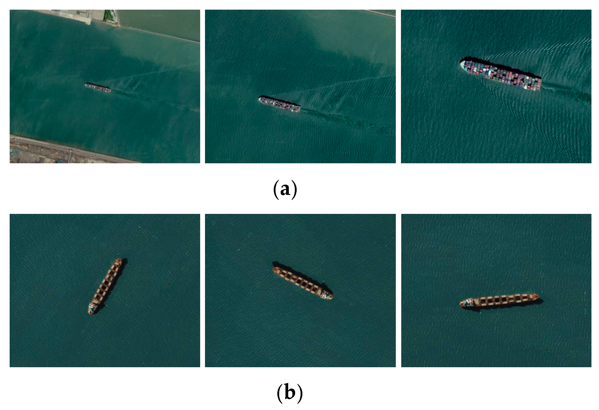
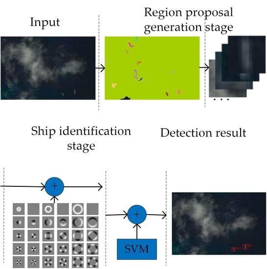
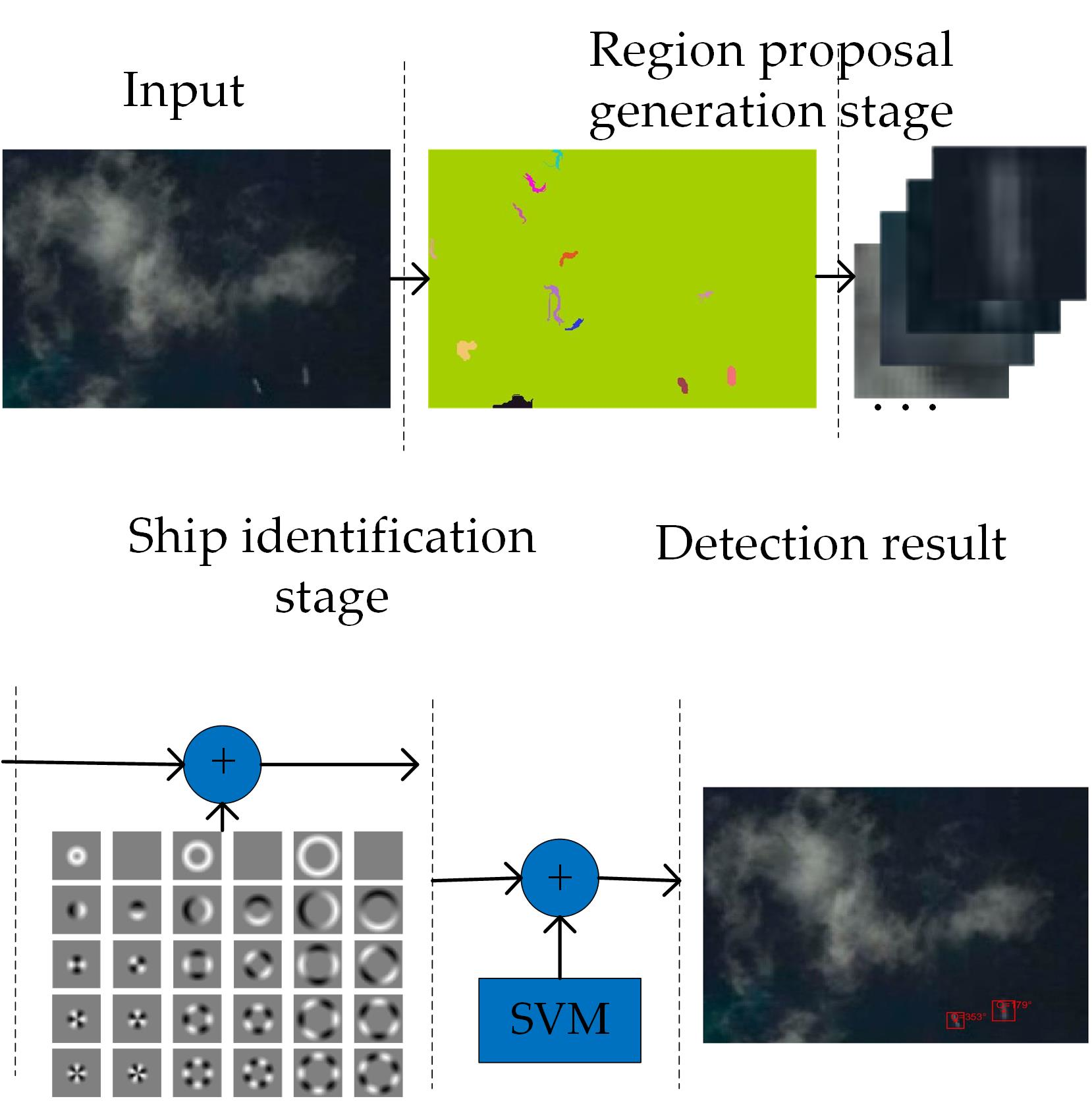
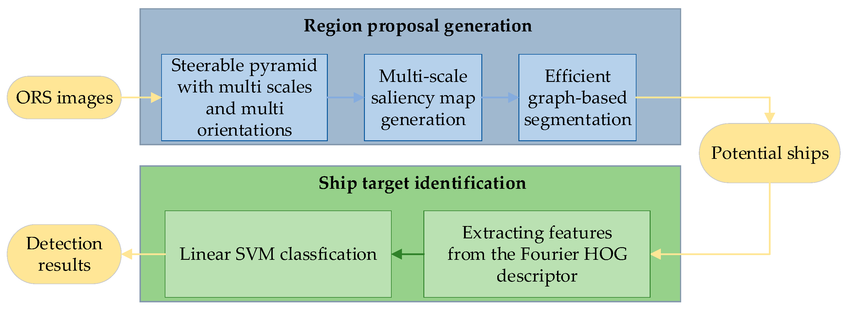
There are two typical challenges for ship detection in ORS images. They are scale and rotation, as illustrated in Figure 1. To overcome these two issues, a robust and practical multi-stage ship detection algorithm is presented in this paper. Figure 2 shows the flow chart of the proposed detection scheme.

The scheme contains two stages: region proposal and ship target identification. In the region proposal stage, the luminance channel is decomposed using a steerable pyramid [29] with six orientations and five scales. The difference between the maximum and minimum output of each filter is used as a criterion for the efficiency of the generated saliency map. Then, some saliency maps that may be related to the direction of sea clutter are removed. Unlike other threshold-based methods, the graph segmentation algorithm [30] based on multi-scale saliency maps is constructed to overcome the problem of ship scale change and accurately locate candidate regions. In addition, by selecting efficient saliency maps, the region proposal algorithm can suppress the sea clutter to some extent. In the ship identification stage, the rotation-invariant HOG descriptor [31], using Fourier analysis in polar coordinates, is investigated to distinguish between the targets and the false alarms. Meanwhile, the main direction of the ship can also be estimated in this phase. The proposed detection framework achieves a good detection rate of ship targets in cluttered scenes. In general, our overall detection algorithm may become an effective contributor for improving the performance of the ship detection system.

The remainder of this paper is organized as follows: we state the framework of our candidate region generation algorithm in detail in Section 2. Section 3 introduces the techniques of building the rotation-invariant Fourier HOG descriptor. We demonstrate our experimental results based on the ORS image dataset and compare the results with other detection methods in Section 4. The final Section concludes the paper by summarizing our findings.

2. Region Proposal Algorithm Based on Multi-Scale Analysis

Ship objects in ORS images often appear at very different scales and have large size differences. Besides, they usually have great intensity fluctuations and obvious edges. Based on the above analysis, we can conclude that both the multi-scale decomposition and the differential algorithm are powerful tools for capturing ship characteristics from ORS images. The Steerable Pyramid (SP), which can combine the pyramid decomposition and the derivative operation into a single operation, is introduced to design our region proposal algorithm. In comparison with orthonormal wavelet transform, the SP has some advantages (for example, steerable orientation decomposition; aliasing is eliminated) and is more suitable for detecting targets with different scales and orientations in the cluttered scenes. The SP is an overcomplete, linear, multi-scale, and multi-orientation image decomposition whose filters are derivative operators with different support and orientations. The SP transform is implemented as a filter bank consisting of polar-separable filters in the Fourier domain, to form a tight frame and to prevent spatial aliasing. For simplicity, we describe these filters in the frequency domain. 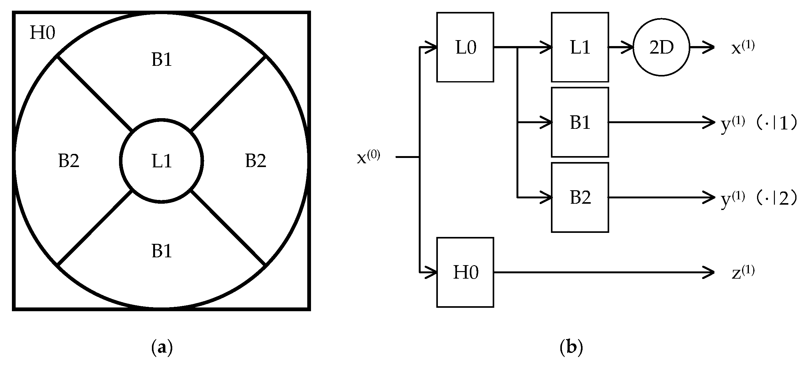Figure 3 shows the frequency tiling of the first level SP decomposition for the case of two orientation bands (i.e., P = 2) and the corresponding diagram. As illustrated in Figure 3a, the frequency plane can be divided into three parts: a low-pass band denoted as L1, two oriented band-pass components denoted as B1 and B2, respectively, and a high-pass band denoted as H0. Figure 3b shows the system diagram for the steerable pyramid. Firstly, the signal x⁽⁰⁾ is pre-separated into the low-pass component by the filter L0 and the high-pass component by the filter H0. The high-pass signal is presented as z⁽¹⁾. The low-pass component is then divided into a set of P oriented detail images y⁽¹⁾(·|p), p = 1,…,P and one approximation signal x⁽¹⁾. The oriented detail images are generated by using the band-pass filters B1,…, BP, while the approximation signal is generated by using the low-pass filter H1 and a dyadic down-sampling process. The approximation signal x^(s−1) can be decomposed into the s-scale oriented images and approximation image.

For a given ORS image, we firstly transform it to the corresponding gray image I⁽⁰⁾ and then define the multi-scale, multi-orientation SP decomposition as follows:

$$\left[I^{(s)}\left\{f_{p,p=1,\dots P}^{(s)}\right\}\right]=SP(I^{(s-1)})s=1,\dots ,S$$

(1)

where s is the decomposition level index, and $s\in \left\{1,\dots ,S\right\}$. The maximum level S used in decomposition is given by $S={\log }_{2}D$ for the input image I⁽⁰⁾ whose largest dimension is size D. p denotes the orientation index, and $p\in \left(1,\dots ,P\right)$. To get more details about the oriented maps, we set P = 6 in this paper. The SP provides a direct representation of the local gradient of the image at different scales. The approximation image I^(s) and the oriented detail image $f_p^{(s)}$ are generated from the s-th level SP decomposition. Note that the filters must satisfy specific radial and angular frequency constraints [29]. After the SP decomposition, the feature map $f_p^{(s)}$ at the S scale and the P orientation is obtained. Let n denote the pixel index in the feature map, and $n\in \left(1,\dots ,N\right)$. N presents the total pixels in the image. We can define our saliency model as:

$$s{c}_p^s(n)=\frac{G_{\sigma }(n)\ast \exp \left(\left|f_p^s(n)\right|\right)}{\frac{1}{N}{\displaystyle \sum _{n=1}^N{G}_{\sigma }(n)\ast \exp \left(\left|f_p^s(n)\right|\right)}}$$

(2)

where $\sigma$ is the standard deviation of the Gaussian filter, and $s{c}_p^s(n)$ denotes the saliency score of pixel n at scale s and orientation p. The current existing ship detection algorithms based on saliency are more effective in quiet sea conditions, and they perform poorly when the scenes include strong sea clutter interferences. It is observed that the sea clutter in an image has the same orientation, and the saliency maps generated by the SP can reflect the orientation information. Based on the above analysis, we design a selection mechanism to eliminate the interference of the sea clutter. According to the selection mechanism, the oriented saliency maps related to the sea clutter are removed, and the remaining saliency maps are used for the subsequent processing. 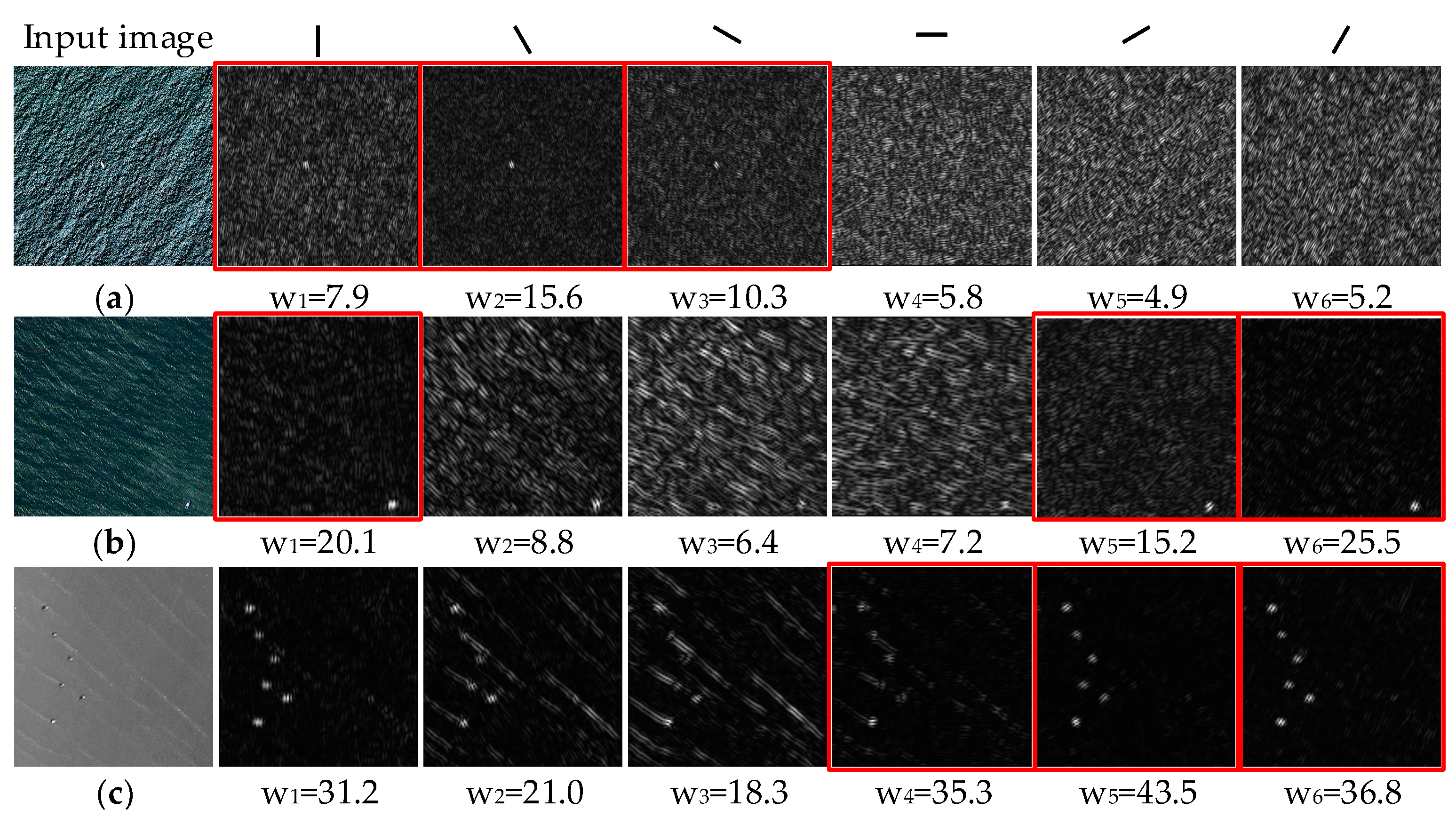Figure 4 shows the generated saliency maps based on the 3-level SP decomposition. The first column presents the test ORS images with strong sea clutter. The remaining columns present their corresponding orientation saliency maps. An efficiency weight $w_p^s$ is calculated for each saliency map $s{c}_p^s$, which is estimated by the difference between the maximum and minimum values of $s{c}_p^s$:

$$w_p^s=\max (s{c}_p^s)-\min (s{c}_p^s)$$

(3)

If the orientation parameter p is consistent with the direction of the sea clutter, the corresponding efficiency weight $w_p^s$ is lower compared to the weights of other orientation saliency maps. Given a set of orientation saliency maps with fixed scale s, we rank them in descending order according to their weights and then preserve the first three saliency maps denoted as $s{c}_{p,p=1,2,3}^{\prime s}$ for subsequent segmentation and region extraction. The remaining saliency maps are marked with red boxes, as shown in Figure 4. These saliency maps can detect the ship targets accurately, even in a highly cluttered background.

In order to extract candidate regions, most existing methods adopt the Otsu segmentation algorithm. The saliency map is binarized by setting any pixels larger than the optimal threshold generated by the Otsu algorithm to one and the rest of pixels to zero. According to the binary map, the regions covered by the bounding rectangles of each connected area are defined as the suspected target regions. However, the threshold segmentation algorithm has two main drawbacks:

• Due to the lack of the spatial structure information, it may introduce the inner holes and could not maintain the integrity for targets.
• There may not be any object of interest present in the target image, so the threshold segmentation may lead to false alarms for such images.

In consideration of these drawbacks, we modify the graph-based segmentation [30] to extract the ship candidates. The proposed graph-based segmentation algorithm can accurately separate the ship targets and backgrounds. Moreover, it can generate a rather smaller set of candidates in comparison with other region proposal algorithms. We describe the modified segmentation algorithm in detail.

Firstly, let G = (V, E) be an undirected graph with vertices $v_i\in V$, the set of elements to be segmented, and edges $\left(v_i,v_j\right)\in E$ corresponding to pairs of neighboring vertices. We define a corresponding weight $w\left(v_i,v_j\right)$ for each edge, which represents the dissimilarity between $v_i$ and $v_j$. In the case of the saliency map segmentation, the set V denotes all the pixels in the saliency map. Let us define the dissimilarity of $v_i$ and $v_j$ as:

$$w\left(v_i,v_j\right)=\sqrt{{\displaystyle \sum _{s=1}^S{\displaystyle \sum _{p=1}^3{\left(s{c}_p^{\prime s}(v_i)-s{c}_p^{\prime s}(v_j)\right)}^2}}}$$

(4)

Note that the saliency map at each scale is resized to the scale of the original image. The more similar the salient values of the two pixels are, the more likely they are to be segmented into the same component. The internal difference of component C is defined as the largest weight in the minimum spanning tree of the component and is denoted as D_int(C). The difference between two components, C and C’, is the minimum weight edge connecting the two components and is denoted as D_ext (C,C’). Besides, the minimum internal difference, MD_int (C,C’), is defined as:

$$M{D}_{\mathrm{int}}\left(C,C^{\prime }\right)=\min \left(D_{\mathrm{int}}\left(C\right)+\frac{k}{\left|C\right|},D_{\mathrm{int}}\left(C^{\prime }\right)+\frac{k}{\left|C^{\prime }\right|}\right)$$

(5)

where $\left|\mathrm{C}\right|$ is the size of component C and $\left|{\mathrm{C}}^{\prime }\right|$ is the size of component C’. k is the constant parameter. Generally speaking, too small k value may cause the over-segmentation. We empirically set k = 800 based on the analysis of [30]. To determine whether C and C1 should be merged into one component, a threshold function is defined as:

$$DT\left(C,C^{\prime }\right)=\{\begin{array}{ll}1& if D_{ext}\left(C,C^{\prime }\right)<M{D}_{\mathrm{int}}\left(C,C^{\prime }\right)\\ 0& otherwise\end{array}$$

(6)

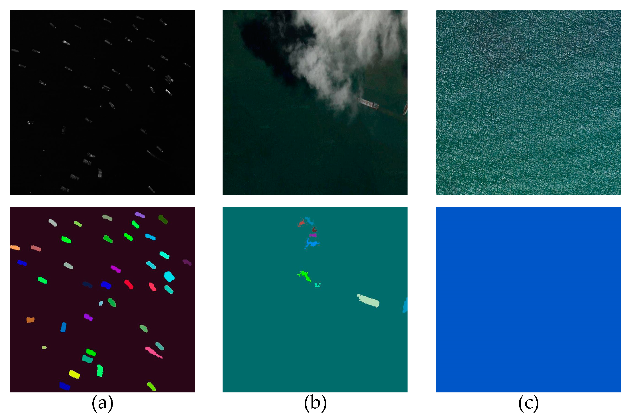
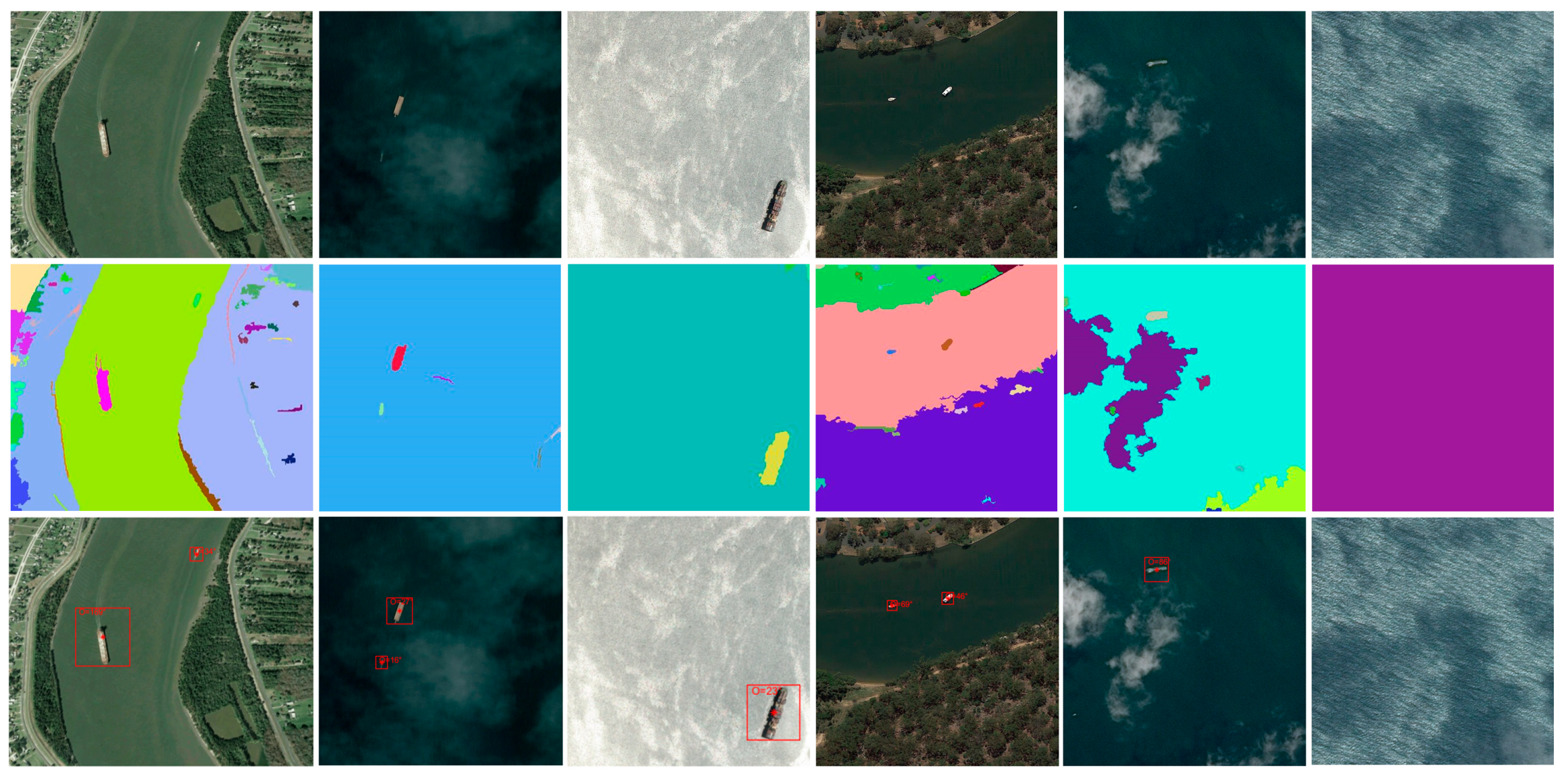
If $DT\left(C,C^{\prime }\right)=1$, then the component C and C’ are merged into one component. By performing this strategy, the segmentation is neither too coarse nor too fine. Since the ship region accounts for a small proportion of the ORS image, we regard the segmented component whose size accounts for more than 40% of the image as the background. As shown in the first column of Figure 5, given the ship targets with uneven brightness and low contrast, the segmentation results can still maintain the integrity for the ships. The second column shows that the proposed region proposal algorithm can detect all ship targets accurately, even under the cloud disturbance. In addition, the algorithm can suppress false alarms to some extent when there is only a quiet sea background and no ship targets in the ORS image, as shown in the last column. To sum up, the modified graph-based segmentation algorithm based on the multi-scale saliency maps can overcome the shortcomings of the low target integrity, the missed detection, and the high false alarm rate. However, due to the lack of prior information in the region proposal algorithm, we need to design the target identification algorithm, which can further remove the false alarms, such as clouds, islands, and strong sea clutters.

3. Rotation-Invariant Feature Extraction Using Fourier Analysis

After performing the region proposal algorithm, the candidate regions can be obtained. They fall into two categories: real ships and false alarms. The aim of the discrimination stage is to distinguish between the real targets and false alarms. Since ship candidates appear in very different directions, we use a rotation-invariant gradient descriptor based on Fourier analysis combined with linear SVM classifier to identify ship targets at arbitrary orientations. This descriptor treats the orientation histograms as continuous functions defined on a circle and uses the Fourier analysis [31] to represent them. Besides, according to the Fourier smoothing histogram, the main orientation of the ship can also be obtained.

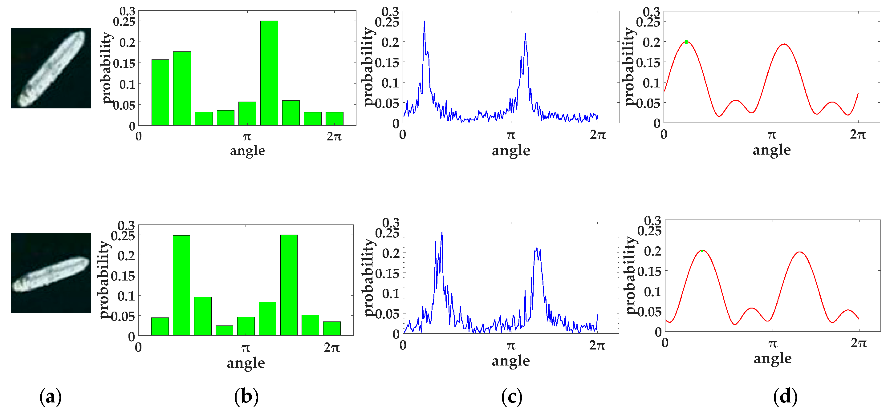
Simply, the HOG feature uses a discrete orientation histogram of an image to describe the shape of the object. In order to obtain the discrete orientation histogram, the gradient magnitude and orientation of each pixel in the image are calculated. Then, the $0-2\pi$ angle range is quantified into several angle intervals. According to the gradient orientation of the pixel, the sum of gradient magnitude of all the pixels falling in the angle interval is counted. Finally, a discrete magnitude-weighted orientation histogram is formed to describe the approximate shape of an object. However, when the image patch rotates, the discrete orientation histogram changes in a complex manner (Figure 6b). Since the continuous orientation histogram $h\left(\xi \right)$ is a period of orientation with a period of $2\pi$, $h\left(\xi \right)$ can be expressed by using its Fourier series coefficients:

$$h\left(\xi \right)={\displaystyle \sum _{m=-\infty }^{\infty }{c}_m{e}^{im\xi }}$$

(7)

with coefficients $c_m=\langle h,e^{im\xi }\rangle =\frac{1}{2\pi }{\displaystyle {\int }_0^{2\pi }h\left(\xi \right)}{e}^{-im\xi }d\xi$, where $m\in \mathbb{Z}$. Let the gradient estimated for each pixel x in the candidate image $I$ be $g\left(x\right)\in {ℝ}^2$, then the gradient distribution function of angle $\xi$ for this pixel can be expressed as a Dirac function with magnitude $\Vert g\left(x\right)\Vert$ and orientation $\angle g\left(x\right)$. According to Equation (7), the Fourier coefficients for $h\left(x,\xi \right)$ read as

$$c_m\left(x\right)=\langle h\left(x,\xi \right),e^{im\xi }\rangle =\Vert g\left(x\right)\Vert e^{-im\angle g\left(x\right)}$$

(8)

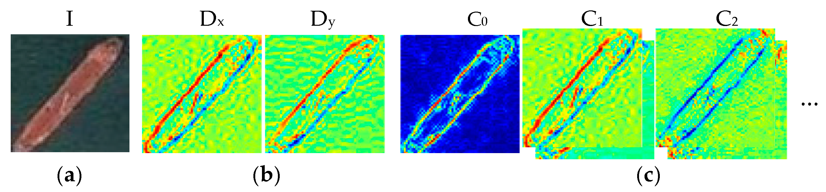
where $m\in {\mathbb{Z}}_{0,M}$, M is the largest order used to describe the image gradient. According to the gradient images, a set of complex-valued coefficient images $\left\{C_m\right\}$ is produced. An example of this expansion is shown in Figure 7.

In practice, the maximum frequency order M is limited to represent the gradient function more smoothly, which can improve the robustness of the gradient histogram when the appearance of the target changes. The orientation histogram of the images can be obtained by summing the orientation histograms of all the individual pixels in the images. Due to the linearity of the Fourier series representation, this can be achieved directly by accumulating coefficients on each extended coefficient image. That is to say, by limiting the value of M, we can get the smoothed orientation histogram $h^{\prime }\left(\xi \right)$, which is defined as follows:

$$h^{\prime }\left(\xi \right)={\displaystyle \sum _{x\in I}{\displaystyle \sum _{m=0}^M{c}_m\left(x\right)}}{e}^{im\xi }$$

(9)

In our implementation, we set M = 4. The vertical direction is defined as zero degrees, and the orientation range is [0,360]. Then, the Fourier smoothing histogram can be obtained, as shown in Figure 6d. Then, the main direction ${\xi }_{main}$ can be estimated as:

$${\xi }_{main}=\underset{{\xi }_n\in \left[0^{\circ },1^{\circ },\dots ,{360}^{\circ }\right]}{\arg \max }{h}^{\prime }\left({\xi }_n\right)$$

(10)

If the discrete gradient histogram is used to calculate the main direction, only the approximate angle interval of the main direction can be obtained (as shown in Figure 6b). If the continuous gradient histogram is directly used to calculate the main direction, the results are easily disturbed by noise and small deformation (as shown in Figure 6c). Some degree of smoothing is beneficial because it increases the robustness of the description to small changes in appearance. Therefore, the smoothed orientation histogram is employed to estimate the main orientation of the ship, which makes the result more stable and accurate (as shown in Figure 6d).

In order to obtain more abundant representations of a circular coefficient image patch, it is integrated against different circular basis functions. Then, the rotation invariance analysis is carried out to extract the final rotation-invariant features.

Since the polar coordinates can separate the angular part from the radial part, which is naturally invariant to rotations, we use polar coordinates to represent each pixel in the image to ensure that the spatial aggregation process is rotation-invariant. Let r denote radial coordinate, let $\theta$ denote angular coordinate; thus, the Fourier coefficient image can be denoted as $C_m\left(r,\theta \right)$. For simplicity, we set the center of the image as the origin of polar coordinates. The basis function $u\left(r,\theta \right)$ is the product of an arbitrary radial profile and a Fourier series basis. The general form is as follows:

$$u_{j,k}\left(r,\theta \right)=p_j\left(r\right)e^{ik\theta }$$

(11)

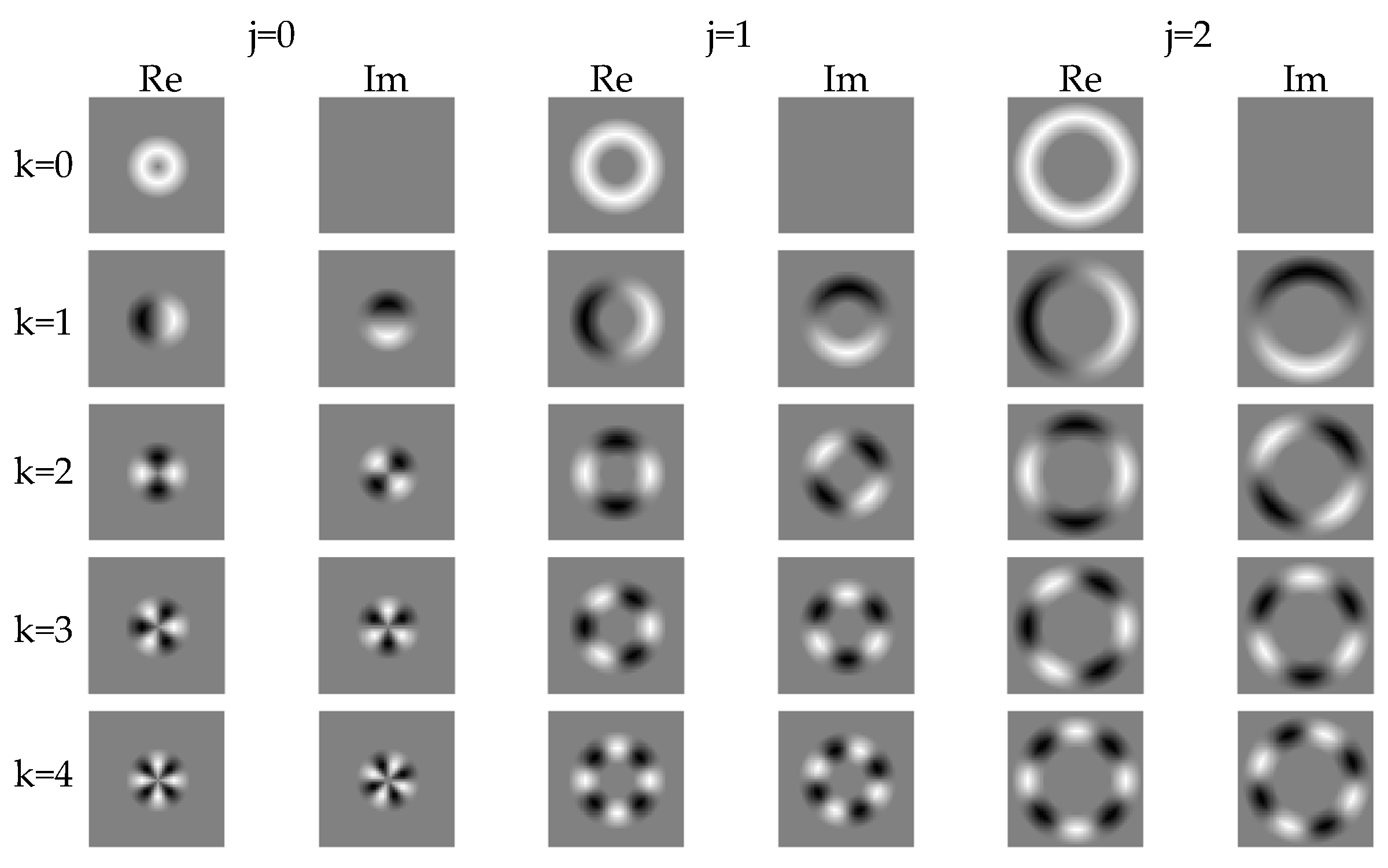
where the integer k denotes the rotation order of the basis function, $k\in \left[-K,K\right]$. The integer j denotes the index of the triangular profile, $j\in \left[0,J-1\right]$. Let R denote the largest radius of basis function, let J denote the number of different profiles, then a set of J profile is defined by:

$$p_j\left(r\right)=\max \left(1-\frac{\left|r-j\sigma \right|}{\sigma },0\right),\sigma =\frac{R}{J}$$

(12)

A set of the circular basis functions is created by using different profiles and Fourier series, an example set of rotation-invariant basis functions with J = 3 and K = 4 is shown in Figure 8.

Next, each basis function $u_{j,k}\left(x\right)$ is convolved with the Fourier coefficient images $c_m\left(x\right)$. The result of convolution can be expressed as:

$$f_{j,k,m}\left(x\right)=u_{j,k}\left(x\right)\ast c_m\left(x\right)$$

(13)

In practice, only the feature set $f_{j,k,m}\left(x_0\right)$ of the center point $x_0$ in the candidate region need to be extracted for further classification. When the underlying image patch rotates by an angle $\varphi$, the resulting complex feature value undergoes a phase shift of $\stackrel{\wedge }{k}\varphi$, where the feature rotation order $\stackrel{\wedge }{k}=k-m$. Consequently, the complex magnitudes of these complex feature values are rotation-invariant. Note that for m = 0, $c_0\left(x\right)$ is a real-valued quantity, $f_{j,k,0}=\overline{f_{j,-k,0}}$ and, therefore, only the basic functions with $k\ge 0$ are adopted to avoid redundancy in the feature set. The final rotation invariant feature vector consists of four parts: the real and imaginary parts of complex features where $\stackrel{\wedge }{k}=0$ and $m\ne 0$, the purely real features with m = k = 0, the magnitude of all other features $\stackrel{\wedge }{k}\ne 0$, and the derived features created by coupling the raw features to give quantities that encode relative phase information [31]. Note that only the lower degrees $-4\le \stackrel{\wedge }{k}\le 4$ are considered. In our experiment, we set the training set patch size to 63✕63, $M=4,K=4,J=3$. 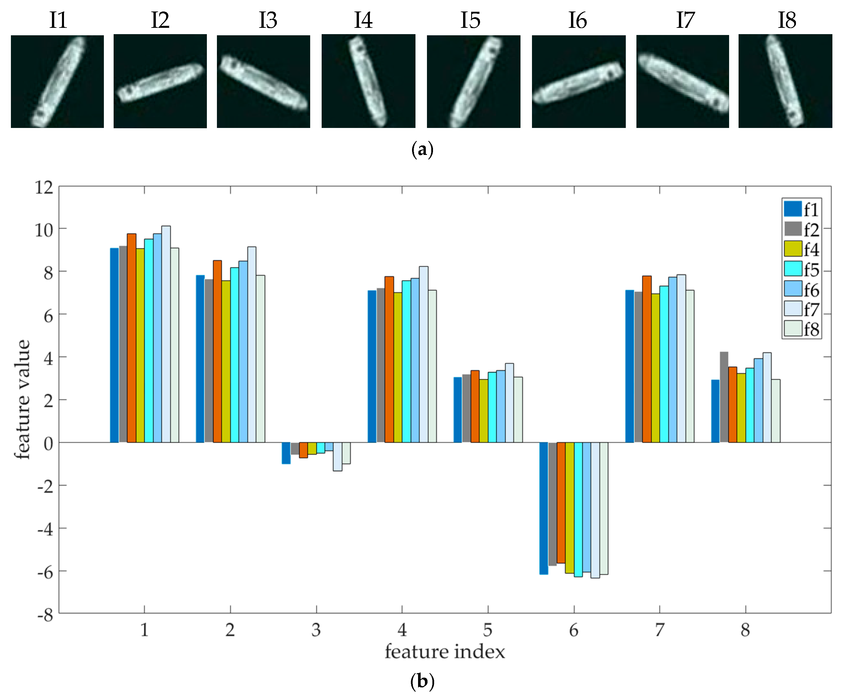Figure 9 demonstrates the effectiveness and robustness of the extracted rotation-invariant feature vector.

After extracting the rotation-invariant feature vector of the candidate image, a linear SVM classifier [31] is adapted to determine whether the candidate region is a ship or a false alarm. To work with the linear SVM, each feature dimension is normalized into the range [−1,1].

4. Experimental Results and Discussion

Firstly, we compare our saliency model with state-of-the-art methods. In addition, we compute the receiver operating characteristic (ROC) area under the curve (AUC) metric to quantitatively evaluate the performance. Next, the effectiveness of the rotation-invariant feature built by the Fourier analysis is validated. Finally, some experiments are conducted to further demonstrate the effectiveness and robustness of our overall detection system.

4.1. Data Set Description

In experiments, we applied the ORS images collected from Google Earth to test the performance of the proposed offshore ship detection scheme. The dataset was carefully selected to mostly cover all possible image conditions, for example, different illumination, scales, and backgrounds, such as quiet sea surface, clouds, fog, strong sea clutters, etc. It had 625 ORS images containing 1248 ships. We randomly divided 625 images into two groups. The first group contained 500 ORS images. They were used for candidate region generation by performing our region proposal algorithms. The second group consisted of 125 ORS images. They were used for testing the overall ship detection scheme. A total of 1248 ships were manually annotated with bounding boxes. Besides, the binary images were also provided for saliency model validation. Some typical ORS images in the dataset are shown in Figure 10.

4.2. Qualitative and Quantitative Saliency Model Evaluation

This section evaluates the performance of our saliency model. Figure 10 and Figure 11 compare our results with the RARE2012 model [32] and the spectral residual (SR) model [33] in various types of sea backgrounds. The RARE2012 model contains three main steps. First, the low-level color and medium-level orientation features are extracted by using a set of Gabor filters. Second, a multi-scale rarity mechanism is designed. Finally, the rarity maps are fused into a single saliency map. The SR model computes the saliency map in the frequency domain; thus, it is independent of any feature. In this method, the image Fourier spectrum is computed firstly. Then, the log-spectrum of the Fourier spectrum map can be obtained. The spectral residual map is obtained by subtracting the log-spectrum map and its smooth version. The final saliency map is generated by Fourier transform inversion. To compare with the two models mentioned above, we used the sum of the multi-scale saliency maps generated by the SP decomposition as the saliency map of our model. We present the results of the three saliency approaches in the case of the quiet sea, the cloudy sea, and the strong sea clutters. The generated saliency maps are shown in Figure 10.

We can draw the conclusion that all saliency models can accurately extract ROIs in the quiet sea background, which verifies the effectiveness of the saliency models in extracting ROIs from the ORS images. When the background becomes complex (such as clouds, strong sea clutters, etc.), as shown in Figure 10b,c, the accuracy of all the saliency models in predicting the locations of the salient targets decreases. Nevertheless, our model has better robustness than the other two saliency models. It can be observed from Figure 11 that the RARE2012 model and the SR model ignore the finer details of the salient region, as both the methods calculate the saliency by adjusting the size of the original image. In addition, when the targets are close to each other, the two models merge different targets together, so that the accurate locations of the different targets cannot be obtained. Besides, compared with our saliency model and SR model, RARE2012 model performs poorly in suppressing the complex background. In general, our saliency model has the following advantages:

• Our saliency model highlights the salient regions along with the fine details effectively and can accurately locate the regions of interest.
• It has a strong ability to suppress complex background and is robust to the interference of the various sea background.
• It can uniformly highlight all the objects in the ORS images, even though some of them have very low contrast.

In quantitative evaluation, we plot the ROC curve and calculate the AUC value in Figure 11a,b, respectively. The saliency maps are binarized at each threshold within the range [0,255], the true positive rate (TPR) and the false positive rate (FPR) are computed with respect to the ground truth data. In the ROC graph, the TPR is plotted on the Y-axis, and the FPR is plotted on the X-axis. The AUC indicates how well the saliency map predicts the locations of the targets. The larger the AUC value is, the more accurate the prediction result is. Note that the proposed saliency model achieves the highest ROC-AUC performance. It can be concluded that our saliency model is more accurate than other methods.

4.3. Discrimination Results

After performing the saliency detection and the graph-based segmentation, a total of 7324 candidate regions are obtained. It contains 991 ship targets, and the rest are false alarms. Since these false alarms will be removed in the discrimination step, the high number of false alarms is not a serious issue. We randomly selected 1141 false alarms as negative samples for feature extraction and classification. The real ship targets and the selected false alarms are used to verify the discrimination algorithm. Figure 12 shows some examples of the generated candidate regions. Note that the sizes of all candidate ships are adjusted to 63 × 63 for feature extraction.

To demonstrate the feasibility of the Fourier HOG feature, it is compared with the HOG feature and another rotation-invariant feature used in method [17]. Specifically, the HOG feature characterizes the shape information by using histograms of orientation gradient. The rotation-invariant feature proposed by the method [17] describes the objects in terms of the shape and texture information. The three different features are combined with the linear SVM classifier and use the same dataset for training and testing. We employ the precision-recall (PR) curve and the classification accuracy to quantitatively measure the performance. The classification accuracy is defined as the ratio of the number of correctly classified samples to the total number of tested samples. A comparison of the PR curve is shown in Figure 13a, and the classification accuracy is presented in Figure 13b.

The reason for the poor performance of the HOG feature is that most of the ships in the ORS images have various orientations, and the HOG feature is sensitive to the target orientation. Compared with the feature used in method [17], the Fourier HOG feature transforms the gradient information into the frequency domain. It can be concluded that the Fourier HOG feature has more powerful description ability in terms of the PR curve and the classification accuracy. It is feasible to apply the Fourier HOG feature to the ship target description.

4.4. Validation of Overall Detection Performance

In experiments, we apply the remaining 125 ORS images containing 252 real ships to test the performance of the proposed ship detection scheme. The accuracy ratio $Ar$ and the false ratio $Fr$ are employed as performance metrics, defined as:

$$Ar=\frac{Nd}{Nts}\times 100\%$$

(14)

$$Fr=\frac{Nfa}{Nd+Nfa}\times 100\%$$

(15)

where $Nd$ is the number of correctly detected ships. $Nts$ is the total number of real ships. $Nfa$ is the number of false alarms. The overall detection algorithm is divided into two stages. The results of the candidate region extraction stage and the target identification stage are shown in

Table 1. Detection results of the proposed ship detection scheme.

Stage	$\mathit{N}\mathit{d}$	$\mathit{N}\mathit{t}\mathit{s}$	$\mathit{N}\mathit{f}\mathit{a}$	$\mathit{A}\mathit{r}$	$\mathit{F}\mathit{r}$
1	245	252	1646	97%	87%
2	235	252	11	93%	4%

.

According to the detection results of the first stage, although our region proposal algorithm achieves high false ratio, it guarantees the detection accuracy. Next, after the target identification stage, a large number of false alarm targets are removed, and real ship targets are retained. Some typical detection results are displayed in Figure 14. The detected ships are marked with the red boxes.

As shown in Figure 14, our algorithm can accurately detect ship targets, effectively remove false alarms, and estimate the orientation of the ship. The experimental results show the effectiveness and superiority of our detection algorithm. However, there are still a small number of false alarms and missing targets, as shown in Figure 15. One possible reason for missing detection is that the target is too small and the resolution is too low, which is not conducive to extracting stable Fourier HOG features. Besides, when the shape of the false alarm is similar to that of the real ship, it may cause false detection.

5. Conclusions

In this paper, we have proposed a two-stage ship detection algorithm, which solves two typical problems of scale and rotation change in complex background. Firstly, in the region proposal stage, the multi-scale and multi-orientation steerable pyramid is employed to generate a set of saliency maps. Then, the set of saliency maps is used for constructing the graph-based segmentation. Compared with the threshold segmentation algorithm, the graph-based segmentation can extract candidate regions more completely and accurately. This stage achieves 97% accuracy ratio, which demonstrates the stability and superiority of the region extraction algorithm. Secondly, in the false alarm rejection stage, the Fourier HOG feature and linear SVM classifier are combined to further eliminate the false alarms and retain the real ships. In addition, the main orientation of the ship can also be estimated. The overall detection scheme achieves 93% accuracy ratio and 4% false ratio. In conclusion, the proposed ship detection algorithm may become an effective contributor to improving the performance of the ship detection system.

It is observed that our model identifies the ship and its wake as a whole. In our future work, we plan to design an effective segmentation algorithm to separate the ship hull from its wake, which will obtain a more accurate target location.

References

1. Zhu, C.R.; Zhou, H.; Wang, R.S.; Guo, J. A Novel Hierarchical Method of Ship Detection from Spaceborne Optical Image Based on Shape and Texture Features. IEEE Trans. Geosci. Remote Sens. 2010, 48, 3446–3456. [Google Scholar] [CrossRef]
2. Leng, X.G.; Ji, K.F.; Xing, X.W.; Zhou, S.L.; Zou, H.X. Area Ratio Invariant Feature Group for Ship Detection in SAR Imagery. IEEE J. STARS 2018, 11, 2376–2388. [Google Scholar] [CrossRef]
3. Zhou, H.T.; Zhuang, Y.; Chen, L.; Shi, H. Signal and Information Processing, Networking and Computers, 3rd ed.; Springer: Singapore City, Singapore, 2018; pp. 164–171. [Google Scholar]
4. Itti, L.; Koch, C.; Niebur, E. A model of saliency-based visual attention for rapid scene analysis. IEEE Trans. Pattern Anal. Mach. Intell. 1998, 20, 1254–1259. [Google Scholar] [CrossRef] [Green Version]
5. Borji, A.; Cheng, M.M.; Jiang, H.Z.; Li, J. Salient Object Detection: A Benchmark. IEEE Trans. Image Process. 2015, 24, 5706–5722. [Google Scholar] [CrossRef] [PubMed] [Green Version]
6. Zhuang, Y.; Qi, B.G.; Chen, H.; Bi, F.K.; Li, L.L.; Xie, Y.Z. Locally Oriented Scene Complexity Analysis Real-Time Ocean Ship Detection from Optical Remote Sensing Images. Sensors 2018, 18, 3799. [Google Scholar] [CrossRef] [PubMed]
7. Zhang, L.B.; Sun, Q.Y. Saliency detection and region of interest extraction based on multi-image common saliency analysis in satellite images. Neurocomputing 2018, 283, 150–165. [Google Scholar] [CrossRef]
8. Xu, F.; Liu, J.H.; Dong, C.; Wang, X. Ship Detection in Optical Remote Sensing Images Based on Wavelet Transform and Multi-Level False Alarm Identification. Remote Sens. 2017, 9, 985. [Google Scholar] [CrossRef]
9. Dalal, N.; Triggs, B. Histograms of Oriented Gradients for Human Detection. In Proceedings of the IEEE Computer Society Conference on Computer Vision and Pattern Recognition, San Diego, CA, USA, 20–25 June 2005; pp. 886–893. [Google Scholar]
10. Yao, Y.; Jiang, Z.G.; Zhang, H.P.; Wang, M.F.; Meng, G. Ship detection in panchromatic images: A new method and its DSP implementation. In Proceedings of the ISPRS International Conference on Computer Vision in Remote Sensing, Xiamen, China, 28–30 April 2015; pp. 1–5. [Google Scholar]
11. Shi, Z.W.; Yu, X.R.; Jiang, Z.G.; Li, B. Ship Detection in High-Resolution Optical Imagery Based on Anomaly Detector and Local Shape Feature. IEEE Trans. Geosci. Remote Sens. 2014, 52, 4511–4523. [Google Scholar]
12. Yang, F.; Xu, Q.Z.; Li, B.; Ji, Y. Ship Detection from Thermal Remote Sensing Imagery through Region-Based Deep Forest. IEEE Geosci. Remote Sens. Lett. 2018, 15, 449–453. [Google Scholar] [CrossRef]
13. Shi, H.; Zhang, Q.J.; Bian, M.M.; Wang, H.Y.; Wang, Z.R.; Chen, L.; Yang, J. A Novel Ship Detection Method Based on Gradient and Integral Feature for Single-Polarization Synthetic Aperture Radar Imagery. Sensors 2018, 18, 563. [Google Scholar] [CrossRef]
14. Qi, S.X.; Ma, J.; Lin, J.; Li, Y.S.; Tian, J.W. Unsupervised Ship Detection Based on Saliency and S-HOG Descriptor from Optical Satellite Images. IEEE Geosci. Remote Sens. Lett. 2015, 12, 1451–1455. [Google Scholar]
15. Zhang, S.; Wu, R.; Xu, K.; Wang, J.; Sun, W. R-CNN-Based Ship Detection from High Resolution Remote Sensing Imagery. Remote Sens. 2019, 11, 631. [Google Scholar] [CrossRef]
16. Wang, G.L.; Wang, X.C.; Fan, B.; Pan, C.H. Feature Extraction by Rotation-Invariant Matrix Representation for Object Detection in Aerial Image. IEEE Geosci. Remote Sens. Lett. 2017, 14, 851–855. [Google Scholar] [CrossRef]
17. Dong, C.; Liu, J.H.; Xu, F. Ship Detection in Optical Remote Sensing Images Based on Saliency and a Rotation-Invariant Descriptor. Remote Sens. 2018, 10, 400. [Google Scholar] [CrossRef]
18. Xu, F.; Liu, J.H.; Sun, M.C.; Zeng, D.D.; Wang, X. A Hierarchical Maritime Target Detection Method for Optical Remote Sensing Imagery. Remote Sens. 2017, 9, 280. [Google Scholar] [CrossRef]
19. Wu, F.; Zhou, Z.Q.; Wang, B.; Ma, J.L. Inshore Ship Detection Based on Convolutional Neural Network in Optical Satellite Images. IEEE J. STARS 2018, 11, 4005–4015. [Google Scholar] [CrossRef]
20. Wang, R.F.; Li, J.; Duan, Y.P.; Cao, H.J.; Zhao, Y.J. Study on the Combined Application of CFAR and Deep Learning in Ship Detection. J. Indian Soc. Remote Sens. 2018, 46, 1413–1421. [Google Scholar] [CrossRef] [Green Version]
21. Cheng, G.; Zhou, P.C.; Han, J.W. Learning Rotation-Invariant Convolutional Neural Networks for Object Detection in VHR Optical Remote Sensing Images. IEEE Trans. Geosci. Remote Sens. 2016, 54, 7405–7415. [Google Scholar] [CrossRef]
22. Gallego, A.J.; Pertusa, A.; Gil, P. Automatic Ship Classification from Optical Aerial Images with Convolutional Neural Networks. Remote Sens. 2018, 10, 511. [Google Scholar] [CrossRef]
23. Zhang, X.; Zhu, K.; Chen, G.; Tan, X.; Zhang, L.; Dai, F.; Liao, P.; Gong, Y. Geospatial Object Detection on High Resolution Remote Sensing Imagery Based on Double Multi-Scale Feature Pyramid Network. Remote Sens. 2019, 11, 755. [Google Scholar] [CrossRef]
24. Li, Q.P.; Mou, L.C.; Liu, Q.J.; Wang, Y.H.; Zhu, X.X. HSF-Net: Multiscale Deep Feature Embedding for Ship Detection in Optical Remote Sensing Imagery. IEEE Trans. Geosci. Remote Sens. 2018, 56, 7147–7161. [Google Scholar] [CrossRef]
25. Ren, S.Q.; He, K.M.; Girshick, R.; Sun, J. Faster R-CNN: Towards Real-Time Object Detection with Region Proposal Networks. IEEE Trans. Pattern Anal. Mach. Intell. 2017, 39, 1137–1149. [Google Scholar] [CrossRef] [PubMed] [Green Version]
26. Liu, W.C.; Ma, L.; Chen, H. Arbitrary-Oriented Ship Detection Framework in Optical Remote-Sensing Images. IEEE Geosci. Remote Sens. Lett. 2018, 15, 937–941. [Google Scholar] [CrossRef]
27. Redmon, J.; Farhadi, A. YOLO9000: Better, Faster, Stronger. In Proceedings of the IEEE Conference on Computer Vision and Pattern Recognition, Honolulu, HI, USA, 21–26 July 2017; pp. 6517–6525. [Google Scholar]
28. Liu, B.Z.; Wu, H.; Su, W.H.; Zhang, W.C.; Sun, J.G. Rotation-invariant object detection using Sector-ring HOG and boosted random ferns. Vis. Comput. 2018, 34, 707–719. [Google Scholar] [CrossRef]
29. Simoncelli, E.P.; Freeman, W.T. The steerable pyramid: A flexible architecture for multi-scale derivative computation. In Proceedings of the International Conference on Image Processing, Washington, DC, USA, 23–26 October 1995; pp. 444–447. [Google Scholar]
30. Felzenszwalb, P.F.; Huttenlocher, D.P. Efficient Graph-Based Image Segmentation. Int. J. Comput. Vis. 2004, 59, 167–181. [Google Scholar] [CrossRef]
31. Liu, K.; Skibbe, H.; Schmidt, T.; Blein, T.; Palme, K.; Brox, T.; Ronneberger, O. Rotation-Invariant HOG Descriptors Using Fourier Analysis in Polar and Spherical Coordinates. Int. J. Comput. Vis. 2014, 106, 342–364. [Google Scholar] [CrossRef]
32. Riche, N.; Mancas, M.; Duvinage, M.; Dutoit, T. RARE2012: A multi-scale rarity-based saliency detection with its comparative statistical analysis. Signal Process. Image Commun. 2013, 28, 642–658. [Google Scholar] [CrossRef]
33. Hou, X.D.; Zhang, L.Q. Saliency Detection: A Spectral Residual Approach. In Proceedings of the IEEE Conference on Computer Vision and Pattern Recognition, Minneapolis, MN, USA, 17–22 June 2007; pp. 2280–2287. [Google Scholar]
Figure 1. Two typical challenges for ship detection in optical remote sensing (ORS) images. (a) Three different scales. The scale change increases the difficulty of the candidate region extraction. (b) Three different rotations. The rotation change increases the difficulty of feature extraction.
Remotesensing 11 01529 g001
Figure 2. Flow chart of the proposed multi-stage detection scheme. The region proposal stage contains the saliency map generation and the graph-based segmentation. The ship identification stage consists of rotation-invariant feature extraction and the candidate classification. ORS: optical remote sensing; SVM: support vector machine; HOG: histogram of oriented gradients.
Remotesensing 11 01529 g002
Figure 3. Frequency tiling and the corresponding system diagram. (a) Frequency tiling after the first level decomposition with P = 2. (b) The corresponding steerable transform. The frequency plane has been decomposed into three parts: a low-pass band, a high-pass band, and two oriented band-pass components. After the Steerable Pyramid (SP) decomposition, the approximation signal x(1), the high-pass signal z(1), and the band-pass signal y(1)(·|p) are obtained.
Remotesensing 11 01529 g003
Figure 4. The generated saliency maps based on the 3-level Steerable Pyramid (SP) decomposition. The first column presents the test optical remote sensing (ORS) images with strong sea clutter. The remaining columns present their corresponding orientation saliency maps. Besides, wp (p = 1,2,..,6) denotes the efficiency weight of the p-th orientation saliency map. A selection strategy is performed to suppress the strong sea clutter. The remaining saliency maps are marked with red boxes.
Remotesensing 11 01529 g004
Figure 5. The optical remote sensing (ORS) images and the corresponding segmentation results. (a) Ship targets with uneven brightness and low contrast. (b) Ship targets disturbed by the clouds. (c) No target in the ORS image.
Remotesensing 11 01529 g005
Figure 6. Different types of gradient histograms. (a) Input image patches with different angles. (b) The discrete gradient histograms. (c) The continuous gradient histograms. (d) The Fourier smoothing gradient histograms with M = 4. The angle value corresponding to the green point is the main direction of the target. The discrete gradient histogram has poor orientation behavior while continuous Fourier smoothing histogram simply shifts cyclically.
Remotesensing 11 01529 g006
Figure 7. The expansion process from the gradient images to the Fourier coefficient images. (a) Input image. (b) Gradient images. (c) The Fourier coefficient images. Note that the real and imaginary parts of the Fourier series are shown separately.
Remotesensing 11 01529 g007
Figure 8. The circular basis functions with J = 3, K = 4(only k 0 displayed).
Remotesensing 11 01529 g008
Figure 9. The demonstration of rotation-invariant features of the ship targets. (a) A series of patches with different angles denoted as Ik (k = 1,..,8). (b) Their corresponding output feature vectors fk. Note that only the first eight feature dimensions are shown in the bar chart.
Remotesensing 11 01529 g009
Figure 10. Qualitative comparison of the saliency models in different types of backgrounds. (a) The calm sea. (b) The cloud cover. (c) The strong sea clutters. SR: spectral residual.
Remotesensing 11 01529 g010aRemotesensing 11 01529 g010b
Figure 11. The receiver operating characteristic- area under the curve (ROC-AUC) performance of the saliency models. (a) ROC curve. (b) AUC value.
Remotesensing 11 01529 g011
Figure 12. Examples of the candidate regions. The real ship targets are presented in the first row. The false alarms are presented in the second row.
Remotesensing 11 01529 g012
Figure 13. PR (precision-recall) curve and classification accuracy for different types of feature. (a) Precision-recall curve. (b) Classification accuracy.
Remotesensing 11 01529 g013
Figure 14. The detection results of our overall detection algorithm. The first row corresponds to the input image. The second row presents the result of the segmentation. The last row is the final detection result after false alarm rejection. Besides, the main orientation of the target is also estimated.
Remotesensing 11 01529 g014
Figure 15. Two failed detection examples. Due to the small target size and low resolution of the ship, missed detection marked with the green box occurs in the first row. In the second row, due to the shape of the island similar to that of the ship, false detection marked with the green box occurs.
Remotesensing 11 01529 g015