Sensitivity Analysis and Minimal Measurement Geometry for the Target-Based Calibration of High-End Panoramic Terrestrial Laser Scanners

Abstract

Target-based calibration is the most widely used calibration procedure for terrestrial laser scanners. Nevertheless, the current implementations of this procedure are suboptimal due to the high complexity of their calibration fields. Therefore, designing calibration fields, by selecting optimal target locations with respect to the instrument, is a pending research question. Answering this question would lead to a more efficient and user-friendly calibration, as well as improved calibration results. Herein, we conduct a detailed analysis of the most sensitive target-to-instrument measurement configuration to estimate individual calibration parameters. Based on this analysis, we derive a minimal measurement geometry, sensitive to all mechanical misalignments, relevant for high-end panoramic terrestrial laser scanners. We support our sensitivity analysis by a simulation and empirical experiments followed by a discussion about the advantages and shortcomings of the proposed minimal measurement geometry.

1. Introduction

Calibration of terrestrial laser scanners (TLSs) is necessary to assure sufficient measurement quality for tasks demanding high accuracy, such as deformation monitoring and reverse engineering [1,2]. Despite the manufacturers’ efforts, the assembly of TLSs is not faultless, and the relations of the internal mechanical components can change over time due to long-term utilization or suffered stress. The resulting mechanical misalignments cause systematic displacements of the measured points, reducing the quality of the point cloud. Hence, these misalignments should be mathematically modeled.

In the last two decades, multiple calibration approaches have been developed using different objects in the instrument’s surroundings, such as cylinders [3], planes [4], paraboloids [5], or specialized targets, either intensity-based black and white planar targets [6], monochrome planar targets [7] or spherical targets [8], to aid in the estimation of calibration parameters. Additionally, automatic feature-based calibration approaches, either relying on 2D image features [9] or on 3D geometrical features [10], were recently introduced, while in the future, the use of learned 3D geometrical features is to be expected, as they are already successfully used for point cloud registration [11]. The improvement of the measurement quality with instrument calibration strongly varies in the literature due to the large variety of calibration approaches and investigated instruments. Typically, the calibration introduces significant improvements of 30% to 80% for the accuracy of range, and horizontal and vertical angular measurements [12].

Target-based self-calibration is the most studied and well accepted of these calibration approaches. It was used in multiple experiments and lead to successful in-situ instrument calibrations [12,13,14,15]. However, all of the experiments described in praxis rely on heavily redundant networks of observations, comprising dozens or hundreds of targets and multiple scanner stations [16]. Although assuring the high quality of the estimated calibration parameters, such approaches lack cost-efficiency in the areas of calibration field assembly, measurement acquisition, and processing. Therefore, the optimization of target-based self-calibration leading to a more cost-efficient and user-friendly calibration is an active research topic.

The documented studies focused on manually reducing the number of targets within empirical experiments [14] or simulation experiments [17]. So far, using automatic data-driven optimization algorithms with clearly defined score functions is not possible due to the high complexity of the problem. To compare, multiple studies were published, focusing on the viewpoint planning of optimal TLS stations with respect to the measured object. These studies tend to simplify the problem in order to reduce computational complexity, mostly by reducing the whole problem from 3D to 2D [18,19,20]. However, such an approach is not suited for TLS calibration since the vertical position of the targets is of high importance.

In order to solve the problem of the optimal design of the TLS calibration field, several steps need to be solved [21]. First, the correct functional model describing the genuine mechanical misalignments and TLS measurements [22,23] must be defined. Second, the stochastic model describing the true measurement uncertainty needs to be known [24]. Without fulfilling the latter two conditions, the solutions of the optimization algorithms aiming at optimizing the measurement configuration (i.e., the optimization of geodetic networks) are biased and lead to wrong conclusions [25]. The third step is adequate problem simplification, which would lead to reduced computational complexity leading to a solvable optimization problem, while the final step is optimization algorithm implementation with carefully selected score functions.

This study presents the third step towards the solution of the problem—a problem simplification. Herein, we conduct a sensitivity analysis of each mechanical misalignment separately. Sensitivity analyses are regularly used to analyze the sensitivity of the measurement geometry with different aims in mind [26,27,28]. Our sensitivity analysis investigates the most suited measurement geometry for estimating each calibration parameter. Two similar analyses were already published, one aiming at improving the measurement geometry for the plane-based [29], and one on the target-based TLS calibration [30]. Our analysis shares the same goal with the latter one. However, the latter analysis focused on a reference field of targets with limited dimensions (4 x 4 m), which was realized with an instrument of superior accuracy in laboratory conditions. Instead, we aim at cost-efficient self-calibration. Hence, we aim to find a solution without any reference information. Although we consider realistic dimensional limitations, we also investigate all possible positions of targets in the instrument’s field of view.

Additionally, to prove the potential of such an analysis, we derived the minimal measurement geometry sensitive enough to reveal all relevant calibration parameters. Such geometry perfectly underlines the difference between a typical calibration field relying on a heavy redundancy and a necessary minimum of carefully selected target locations. We discuss the relevance of the derived measurement geometry with respect to the TLS test-fields proposed in the literature [31,32,33]. Namely, they share a common goal of reaching a high sensitivity towards mechanical misalignments in a cost-efficient manner.

We focus on the calibration of a specific line of instruments—the high-end panoramic TLS Leica ScanStation P-series, more precisely Leica ScanStation P20. By high-end, we mean instruments having high-quality components, including angular encoders with multiple reading heads, which eliminate a considerable amount of overall possible TLS misalignments [22,34]. Therefore, we rely on the functional and stochastic models relevant to the instrument under investigation. We focus on this type of instrument as it is the most often used for tasks demanding high accuracy. The transferability of our results to other TLSs is additionally discussed.

We start from the point of view that it is important to have a measurement configuration that is sensitive to all relevant mechanical misalignments due to two main reasons. First, ignoring some parameters (for which we know they exist in physical reality) by not including them in the functional model can lead to biased parameter estimates. This phenomenon is due to unavoidably high correlations between the calibration parameters [9,35,36]. Additionally, this bias will not be reflected in the covariance matrix of the estimated parameters. Hence, the whole analysis of the parameter quality will be false. Second, although some parameters typically have a small impact on the point cloud quality, a comprehensive calibration should not exclude the possibility that these parameters have an untypically high magnitude in certain cases. Therefore, within this work, we treat all of the parameters as equally important and present the detailed sensitivity analysis for all of them.

To summarize, the two main goals of this study are:

• To find the most sensitive measurement geometry for estimating each individual mechanical misalignment for the instrument under investigation and
• to prove the practicality of the conducted sensitivity analysis by deriving the minimal measurement geometry sensitive to all relevant mechanical misalignments.

The results of this analysis provide a step forward to the design of the optimal TLS calibration field, which will be in the focus of our following publications. This work is structured as follows. The problem statement, a review of the state-of-the-art, and the aims of the study are presented in this section. Section 2 presents the theoretical background of our investigation. Section 3 explains the concept of the conducted sensitivity analysis and provides the solution for each of the mechanical misalignments. Section 4 introduces the minimal measurement geometry and provides both simulated and empirical experiments used for validation and the corresponding discussion. Finally, in Section 5, the main conclusions are drawn.

2. Theoretical Background

This section explains the working principle of panoramic TLSs (Section 2.1), extended with a short explanation of relevant mechanical misalignments (Section 2.2). Afterwards, the functional (Section 2.3) and stochastic (Section 2.4) model of the TLS target-based self-calibration are discussed in detail, as they are used both in the following sensitivity analysis, as well as the experimental validation of the results.

2.1. Instrument Geometry and Angular Parameterization

Panoramic TLSs have three main axes (vertical or standing, horizontal or trunnion, and the collimation axis), which are supposed to be orthogonal in the perfect case (Figure 1a). The main components are the horizontal and vertical angular encoders, the rotating mirror and the electronic distance measurement unit (EDM unit or rangefinder). The EDM unit nearly continuously transmits the laser beams, which are deflected from the 45° inclined rotating mirror and reflected to the sampled points enclosing right angles. The mirror rotates around the horizontal axis and the whole instrument rotates around the vertical axis while the angular encoders record these rotational steps (Figure 1b). These polar measurements (ranges, horizontal, and vertical angles) are automatically recalculated to Cartesian coordinates of the local scanner coordinate system (Figure 1a) [37]. The main distinguishing characteristic of panoramic TLSs in comparison to other TLS types (hybrid and camera TLSs) is their wide field-of-view, which covers the whole 3D volume except a small conical area underneath the instrument [38].

After half of the rotation around the vertical axis, the whole 3D environment is captured in a way that part of the environment is measured from the front side and part from the back side of the instrument. If the instrument’s rotation continues to finish the full circle around the vertical axis, the same scenery is measured again and the parts of the environment measured from the front and from the back are swapped. This measurement principle is called two-face measurements, and it can reveal multiple systematic errors, what is commonly used in the geodetic community for the calibration of total stations, which share similar architecture with TLSs [39].

For the TLS calibration, it is necessary to recalculate the Cartesian coordinates $x_j^i, y_j^i, z_j^i$ back to the ranges, horizontal and vertical angles $r_j^i$, ${\phi }_j^i$, ${\theta }_j^i$ mimicking the original measurements:

$$\begin{gathered} r_j^i=\sqrt{x_j^i{}^2+y_j^i{}^2+z_j^i{}^2} \\ {\phi }_j^i=arctan(\frac{x_j^i}{y_j^i}) \\ {\theta }_j^i=arccos(\frac{z_j^i}{r_j^i}) \end{gathered}$$

(1)

where i denotes the measured point and j denotes the scanner station. The horizontal angles are corrected for quadrants by adding 180° or 360° when required, and the vertical angles are corrected by subtracting the calculated value from 360°, where required. This is only one of the several functional descriptions used in the literature [22,40], where both the horizontal and vertical measurements have values from 0° to 360° [23]. The 0° direction of the horizontal angles is arbitrarily defined on each scanner station, while the 0° direction of the vertical angles coincides with the positive direction of z-axis of the local scanner coordinate system (Figure 1). It should be noted that in the case of the vertical angles, there is a measurement gap in the area underneath the instrument (135°–225°).

2.2. Calibration Parameters

The mechanical misalignments causing systematic errors in TLS measurements can be divided into tilts (rotations) and offsets (translations) of the main instrument components with respect to the ideal case. The tilts have a higher impact on measurement quality because the magnitude of the related systematic errors grows with the distance. On the other hand, the systematic errors of the offsets are constant with respect to the distance and are usually small in magnitude. In the case of the high-end panoramic TLSs, there are 10 relevant mechanical misalignments that can be unbiasedly mathematically modeled with 11 calibration parameters (CPs) [23]:

$$\Delta r_j^i=x_2\sin ({\theta }_j^i)+x_{10}+v_{r_j^i}$$

(2)

$$\Delta {\phi }_j^i=\frac{x_{1z}}{r_j^{i}tan({\theta }_j^i)}+\frac{x_3}{r_j^{i}sin({\theta }_j^i)}+\frac{x_{5z-7}}{tan({\theta }_j^i)}+\frac{2x_6}{sin({\theta }_j^i)}+\frac{x_{1n}}{r_j^i}+v_{{\phi }_j^i}$$

(3)

$$\Delta {\theta }_j^i=\frac{x_{1n+2}cos({\theta }_j^i)}{r_j^i}+x_4+x_{5n}\cos ({\theta }_j^i)-\frac{x_{1z}sin({\theta }_j^i)}{r_j^i}-x_{5z}sin({\theta }_j^i)+v_{{\theta }_j^i}$$

(4)

where $\Delta r_j^i,\Delta {\phi }_j^i,\Delta {\theta }_j^i$ are the measurement errors decomposed on the random noise $v_{r_j^i}$, $v_{{\phi }_j^i},v_{{\theta }_j^i}$ and the calibration parameters (

Table 1. The list of mechanical misalignments relevant for high-end TLSs.

Parameter	Description
x1n	Horizontal beam offset
x1z	Vertical beam offset
x2	Horizontal axis offset
x3	Mirror offset
x4	Vertical index offset (tilt)
x5n	Horizontal beam tilt
x5z	Vertical beam tilt
x6	Mirror tilt
x7	Horizontal axis error (tilt)
x10	Rangefinder offset

). Figure 2 depicts the latter misalignments excluding the commonly known vertical index offset and rangefinder offset. The parameter nomenclature is adopted from the American National Institute of Standards and Technology (NIST), who originally derived the parametrization and proved it as valid in the run-off experiment, where several leading manufacturers were involved [41]. The readers are referred to Muralikrishnan et al. 2015 [22] for more details. In this work, we do not focus on the comprehensive rangefinder calibration (e.g., scale and cyclic errors), as it is best resolved with different calibration approaches [42,43].

2.3. Functional Model of the Target-Based Self-Calibration

The target-based TLS calibration implemented herein is based on the algorithm described in [15], which was originally derived from the photogrammetric bundle adjustment [13]. In short, multiple local coordinate systems associated with each scanner station are simultaneously transformed (registered) in the reference system of choice using a sufficient number of corresponding targets observed from each station:

$${\mathit{f}}_{\mathit{j}}^{\mathit{i}}={\mathit{R}}_{(k,\varphi ,\omega )}^i\mathit{x}\mathit{y}{\mathit{z}}_j^i+{\mathit{T}}_{(X,Y,Z)}^i-\mathit{X}\mathit{Y}{\mathit{Z}}_j^{ref.}=\mathbf{0}$$

(5)

The estimated parameters are separated in the rotation matrix ${\mathit{R}}_{(k,\varphi ,\omega )}^i$ defined with Euler angles $(k,\varphi ,\omega ),$ the translation vector ${\mathit{T}}_{(X,Y,Z)}^i$, the vector of Cartesian coordinates of targets in the reference system $\mathit{X}\mathit{Y}{\mathit{Z}}_j^{ref.}$, and the calibration parameters. The measurement vector from the scanner station i to the target j equals:

$$\mathit{x}\mathit{y}{\mathit{z}}_{\mathit{j}}^{\mathit{i}}=\left[\begin{array}{c}{x}_j^i\\ y_j^i\\ z_j^i\end{array}\right]=\left[\begin{array}{c}(r_j^i+\Delta r_j^i)\sin ({\theta }_j^i+\Delta {\theta }_j^i)\sin ({\phi }_j^i+\Delta {\phi }_j^i)\\ (r_j^i+\Delta r_j^i)\sin ({\theta }_j^i+\Delta {\theta }_j^i)\cos ({\phi }_j^i+\Delta {\phi }_j^i)\\ (r_j^i+\Delta r_j^i)\cos ({\theta }_j^i+\Delta {\theta }_j^i)\end{array}\right].$$

(6)

where the polar measurements $r_j^i$, ${\phi }_j^i$, ${\theta }_j^i$ are treated as observations. In order to estimate the calibration parameters, the errors of the transformation process, $\Delta r_j^i,\Delta {\phi }_j^i,\Delta {\theta }_j^i$, are decomposed on the random part described by the adjustment residuals and the systematic part described by the CPs (Equations (2)–(4)). The algorithm is realized as a least squares adjustment based on the rigorous Gauss–Helmert Model.

If the TLS is equipped with an on-board compensator used to level the scans with respect to the local instrument’s horizon, the direct observations of the rotation angles $k$ and $\varphi$ can be additionally included in the calibration adjustment in the form of the constraints [13]:

$$\begin{gathered} k=k_{\mathrm{observed}}\pm {\sigma }_k, \\ \varphi ={\varphi }_{\mathrm{observed}}\pm {\sigma }_{\varphi } \end{gathered}$$

(7)

where ${\sigma }_k$ and ${\sigma }_{\varphi }$ denote the uncertainty of the compensator measurements.

2.4. Stochastic Model

The stochastic model used herein to describe the measurement uncertainty of the instrument under investigation is derived empirically as described in Medic et al. 2019 [24]. In short, multiple targets are repeatedly observed (10 times each) at different distances (from 1 to 100 m) and with different angles of incidence (from 0° to 45°). Afterward, the measurement uncertainty is derived as the standard deviation of the repeatedly estimated target centers. The derived values for the Leica ScanStation P20 are presented in Figure 3. The instrument’s settings, the selected target type, and the target center estimation algorithm correspond to the ones described in the empirical experiment in Section 4.2.

The calculated standard deviations are expressed as a polar measurement (${\sigma }_r, {\sigma }_{\phi }, {\sigma }_{\theta }$), as they are used as the observations in the calibration adjustment. The standard deviations of horizontal and vertical angle measurements are combined because no significant difference between them was observed. Additionally, the values for different angles of incidence are averaged and combined, as no notable difference was observed. This is opposite to the expectations based on the known uncertainty behavior of the rangefinder measurements [44,45] and contrary to the results from Medic et al. 2019 [24]. However, this result is in accordance with the values presented in Janßen et al. 2019 [46], and the reason this result lies in the improved target design of the newly developed BOTA8 targets used herein [46]. The input values for the stochastic model are linearly interpolated with respect to the TLS-to-target distance from the values given in the figure. For the compensator measurement uncertainty, we rely on the values given in the manufacturer’s specifications (${\sigma }_k={\sigma }_{\varphi }=1^{″}$) [47].

We would like to point out two additional uncertainty sources that are considered for the sensitivity analysis described in Section 3 and which are not considered by the implemented stochastic model. Namely, the implemented stochastic model reflects the instrument’s measurement precision, while the following uncertainties are systematic and can be avoided by a plausible measurement configuration.

First, the range measurements in proximity to the instrument are systematically biased, which is presented in Figure 4. In one of our experiments, we compared the relative TLS range measurements (i.e., the differences between two consecutive range measurements ($\Delta d_{TLS}$)) against a reference instrument ($\Delta d_{ref.}$), a more precisely interferometric displacement sensor, on the comparator track. Such a procedure is a common practice for the calibration and testing of EDM instruments [48], and similar procedures were already used in the case of TLSs [43]. Here, we observed repeatable inconsistencies on the order of several millimeters with respect to the reference, which can be traced up to a distance of three meters from the instrument. Similar results were observed for other instruments (Leica HDS6000 and Z+F Profiler 9012 A [49]), but with different magnitudes and spatial extent.

Second, we observed that the measurements of the points located on the edges of black and white regions on the intensity-based black and white targets are systematically displaced (Figure 5). This systematic displacement can bias the target center estimation procedure and should be considered for tasks demanding high measurement accuracy, such as TLS calibration. Figure 5 shows the systematic point displacement of approximately 5 mm in each direction for a target at a distance of 2.5 m. This effect is strongest in the proximity to the instrument and diminishes with distance. The probable explanation lies in the fact that the manufacturers apply an intensity related range measurement correction to account for known systematic errors in range measurements [50]. This way, it is assured that measurements sampling the white and the black surface of a target fall on the same plane in space. However, if the laser beam footprint partially covers the black and the white surface, the applied correction is inadequate.

Therefore, to mitigate the effect of both the mentioned near-field uncertainty sources, we avoid measurements at distances shorter than three meters in the following experiments.

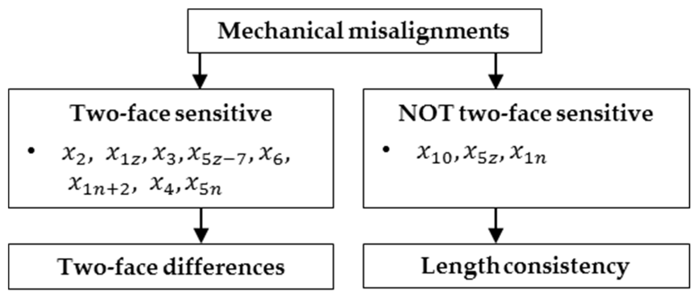
3. Sensitivity Analysis

Concept

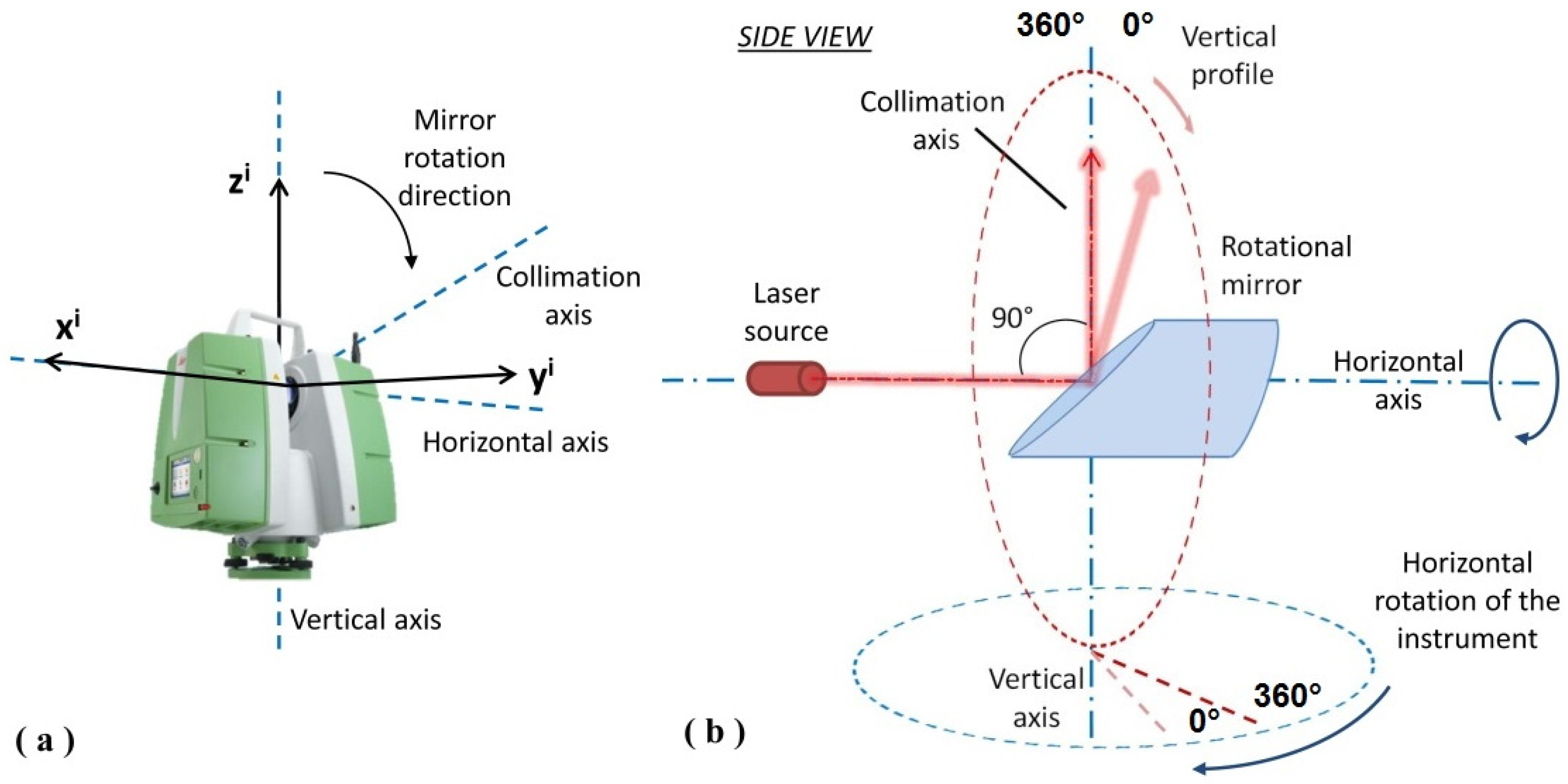
In case of the target-based calibration, there are three main information sources for the detection of systematic measurement errors caused by mechanical misalignments:

• An absolute displacement of a single target (a spatial vector in arbitrary direction within a well-defined coordinate system);
• A length consistency of a test-length (distance change between two targets);
• A difference of two-face measurements of a single target (a vector in the direction of range, horizontal or vertical angle measurements).

From this logic, three different adjustment algorithms for the target-based TLS self-calibration were derived in the literature. Namely, the network-method, the length consistency method, and the two-face method [51].

When conducting the sensitivity analysis, we needed to answer the question: Where should the target or targets be placed in the instrument’s field-of-view so that the misalignment under investigation causes the maximal change? From the difference between the displaced coordinates or deformed length and the reference values, we can calculate the calibration parameter.

The change caused by the misalignment can be considered as a signal, while the uncertainty of estimating the change represents a noise. We need to find relative target(s)-to-TLS positions in which the signal to noise ratio (SNR) is the highest, and, hence, the uncertainty of the estimated calibration parameters is the lowest. Therefore, for the sensitivity analysis, we calculated the mentioned SNR for all possible target-to-TLS positions for each calibration parameter separately. Based on the highest SNR, we discuss the best possible target placement to lead the design of the calibration field. For the analysis, we rely on an accurate functional model of calibration parameters (Section 2.3) and a realistic empirically derived stochastic model of target centroids (Section 2.4).

• The absolute target displacement is the most commonly used information source for TLS calibration in the literature [16,52]. For tracking the spatial target displacement, it is necessary to have the reference target coordinates in a well-defined reference coordinate frame, i.e., it is necessary to define a reference datum. Defining a reference frame requires tremendous effort and can be realized in two different ways: by the bundle adjustment with a strong network of observations or by reference measurements with an instrument of higher accuracy. As we aim at cost-efficient TLS calibration, this information source will not be discussed in more detail.
• Length consistency requires observing a distance between two targets in an arbitrary coordinate system. Hence, it has the potential for a cost-efficient solution. The reference value of a length-test can be realized either with the reference instrument or with an appropriate measurement strategy. Namely, the reference value does not need to reflect the accurate length between two targets. It is sufficient that the length is observed from two TLS positions in the following way: From one position, the misalignment under investigation deforms the length as much as possible, and, from the other position, it deforms it as little as possible. From comparing these two values, it is possible to derive the calibration parameter. The problem of a length test is that a part of the misalignment’s influence can cause a translation or a rotation of the test-length instead of a length change. It is hard to avoid this phenomenon completely. As we do not rely on the known coordinates in a reference coordinate system, the rotation and translation of a length in space cannot be assessed and used for the calibration. Therefore, in many cases, we lose a part of the signal, which impacts the SNR and ultimately the sensitivity of the selected measurement geometry. To calculate the noise, we apply the variance propagation from the target centroid uncertainty to the estimated length of a test-length.
• The last information source, two-face differences, can only be used for estimating two-face sensitive calibration parameters (Figure 6). A misalignment corresponding to such a CP causes a target displacement in a measurement direction that changes its direction if the target is observed on the front side (front face) or the back side (back face) of the instrument, while the magnitude remains the same. Two-face sensitivity depends on a functional connection between the misalignment and the measurements (Equations (2)–(4)). In the case of the ranges and horizontal angles, the CP should switch the sign (due to sine or tangents functions), while in the case of the vertical angles, the sign should remain the same (due to cosines or no function). This rule stems from the way of building two-face differences, which is different for each measurement group [39].

Here, by observing only a single target from a single scanner station, we can detect the doubled value of the signal with comparably low noise—only the TLS measurement’s uncertainty from observing one target. The reference value is simply retrieved as an average of these two observations. The additional advantage is that systematic effects (e.g., incidence angle and refraction) influence both measurements used to form the two-face difference identically (same sign and magnitude). Hence, the difference itself is free of any eventual external systematic effect that could impact the TLS measurements and bias the calibration results.

Fortunately, the majority of the relevant CPs are two-face sensitive. Therefore, for the sake of cost-efficiency, our sensitivity analysis focuses on two information sources that do not require a burdensome definition for the reference frame, i.e., datum-free information sources: the two-face differences for all two-face sensitive parameters and the length-consistency tests for the remaining CPs (Figure 6).

In the following sections, the sensitivity of each calibration parameter relevant for the instrument under investigation is analyzed and the transferability to the other instruments is discussed. Although we consider all possible measurement configurations, we additionally discuss the solutions that are constrained based on the dimensions of the facility that we have at hand for the empirical experiment in Section 4.2 (70 m × 25 m × 9 m).

Realization

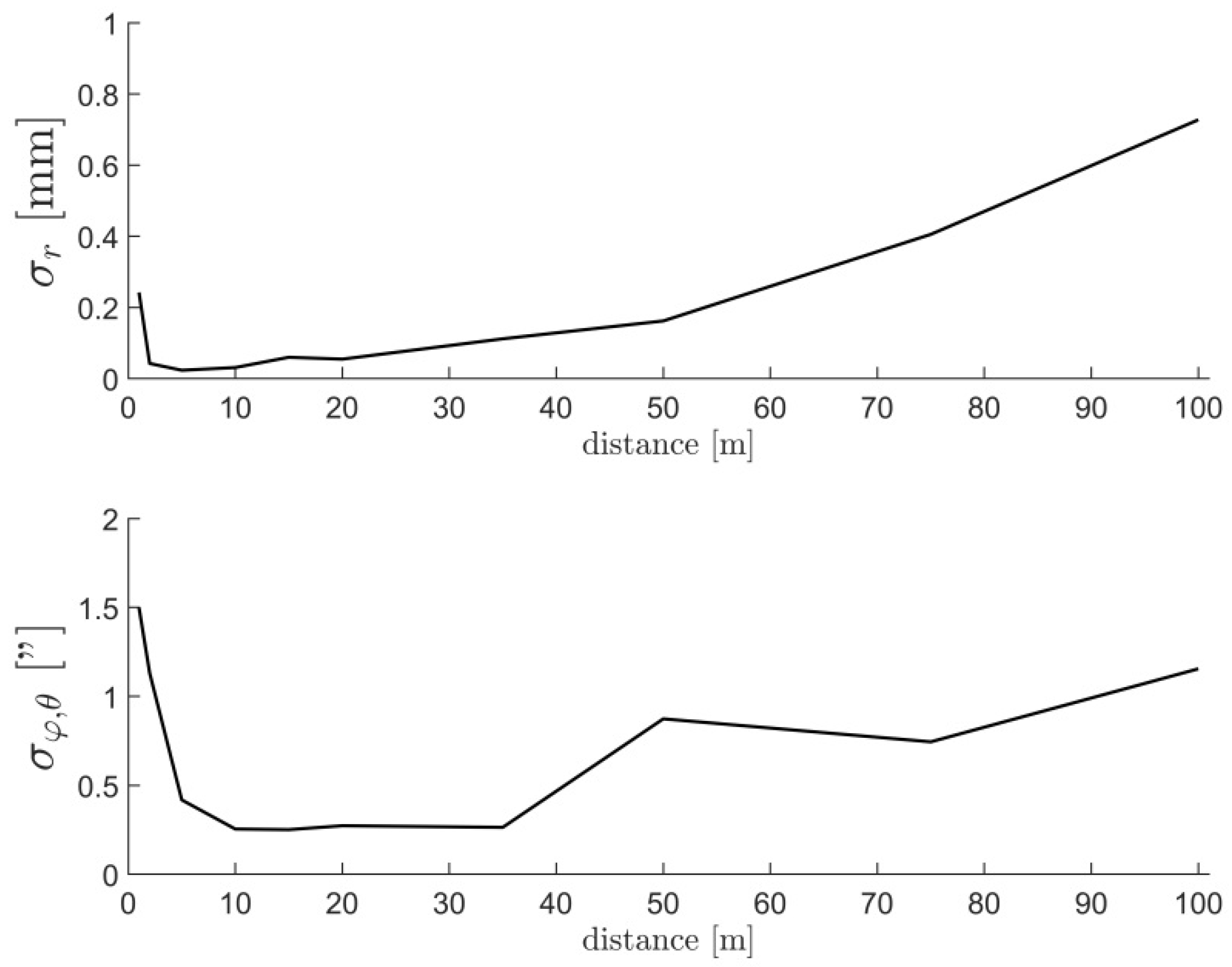
The sensitivity analysis is realized by simulating different target(s)–to–TLS measurement configurations and analyzing the resulting SNR. We made a discretization of all possible target locations within the instrument’s field-of-view. We created a 3D grid of points in the local scanner coordinate system with a resolution of one meter and an extent of 50 m in each direction. We initially selected an extent of 100 m, which is approximately the limit of the successful target center estimation (Section 2.4). However, we reduced this value due to the generally low SNR for locations far away from the instrument. Additionally, we reduced the problem from 3D space to 2D space, where applicable. Sensitivity analysis for some parameters is invariant with respect to the horizontal or vertical position, which simplifies both the computation and visualization of the results.

Finally, we removed all unrealistic measurement configurations. Namely, the measurements with vertical angles between 135° and 225° (around nadir) are impossible due to the limited field-of-view underneath the tripod. Additionally, the measurements with vertical angles between +5° and −5° (around zenith) are again removed due to physical limitations. Namely, because of the target size, it is not possible to place it so close to the zenith while ensuring that the target is not scanned at the same time, both from the front and from the back of the scanner.

The signal to noise ratio is derived as a ratio between the target displacement or the length change in mm and the measurement uncertainty of the target center or estimated length also in mm, and, therefore, it is dimensionless. For generating the signal, i.e., simulating the influence of the mechanical misalignment (Table 1), an impact of 1 arc second for all tilt parameters and 0.1 mm for all offset parameters is used. Therefore, only the SNR within the group (offsets or tilts) are directly comparable, but not between the groups.

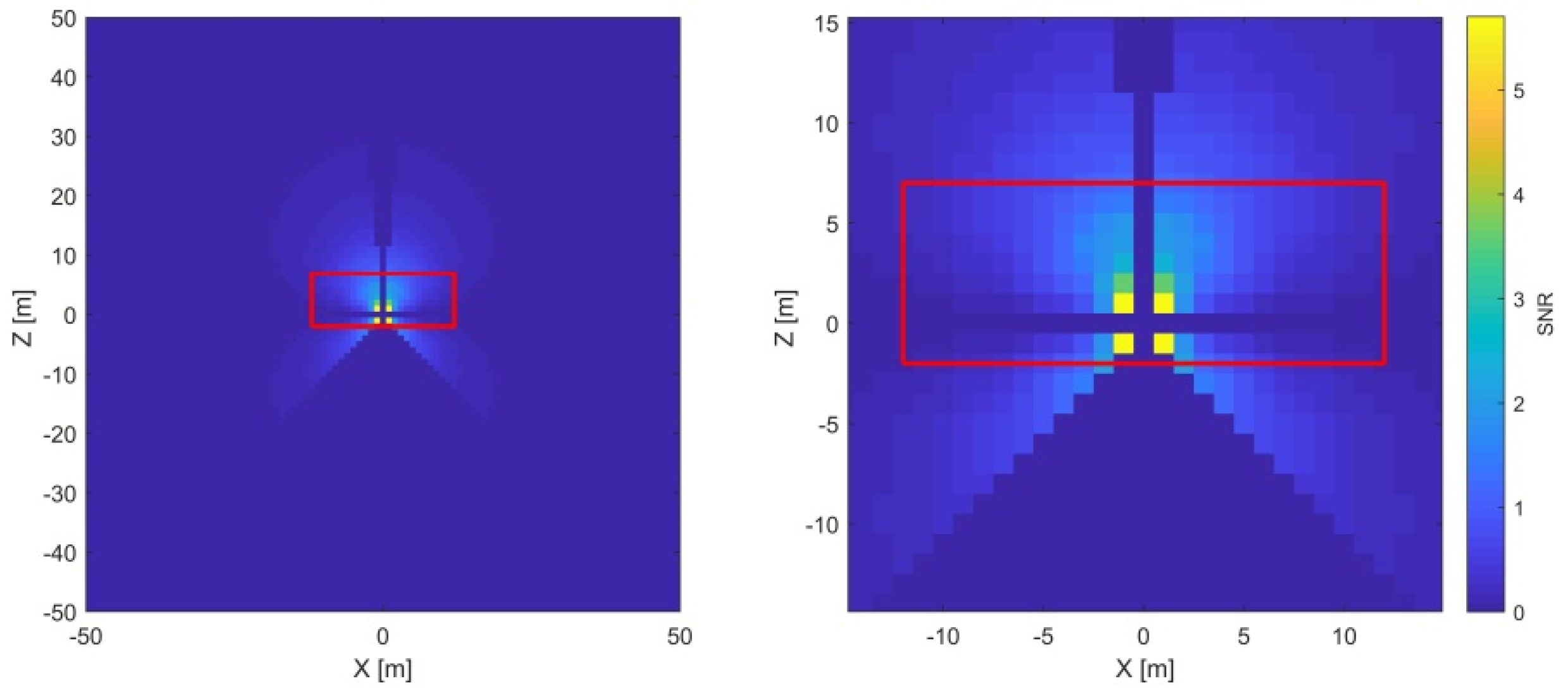
3.1. Sensitivity Analysis of Two-Face Differences

The CPs are ordered by the simplicity of the analysis. The sensitivity analysis of two-face differences is reduced to a 2D case and presented in a vertical plane passing through the origin of the local scanner coordinate system (Figure 7, Figure 8, Figure 9, Figure 10, Figure 11 and Figure 12: X = 0, Z = 0). Namely, the signal of all two-face sensitive mechanical misalignments is invariant to the horizontal angle due to a functional connection with the measurements (Equations (2)–(4)). Each pixel in the following figures represents the target location in the instrument’s field-of-view.

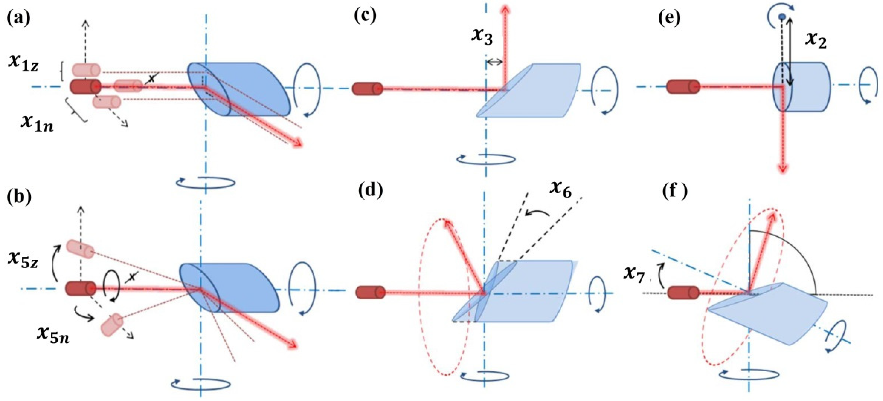
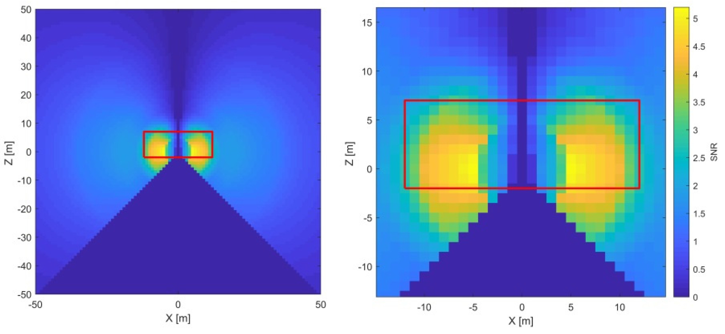
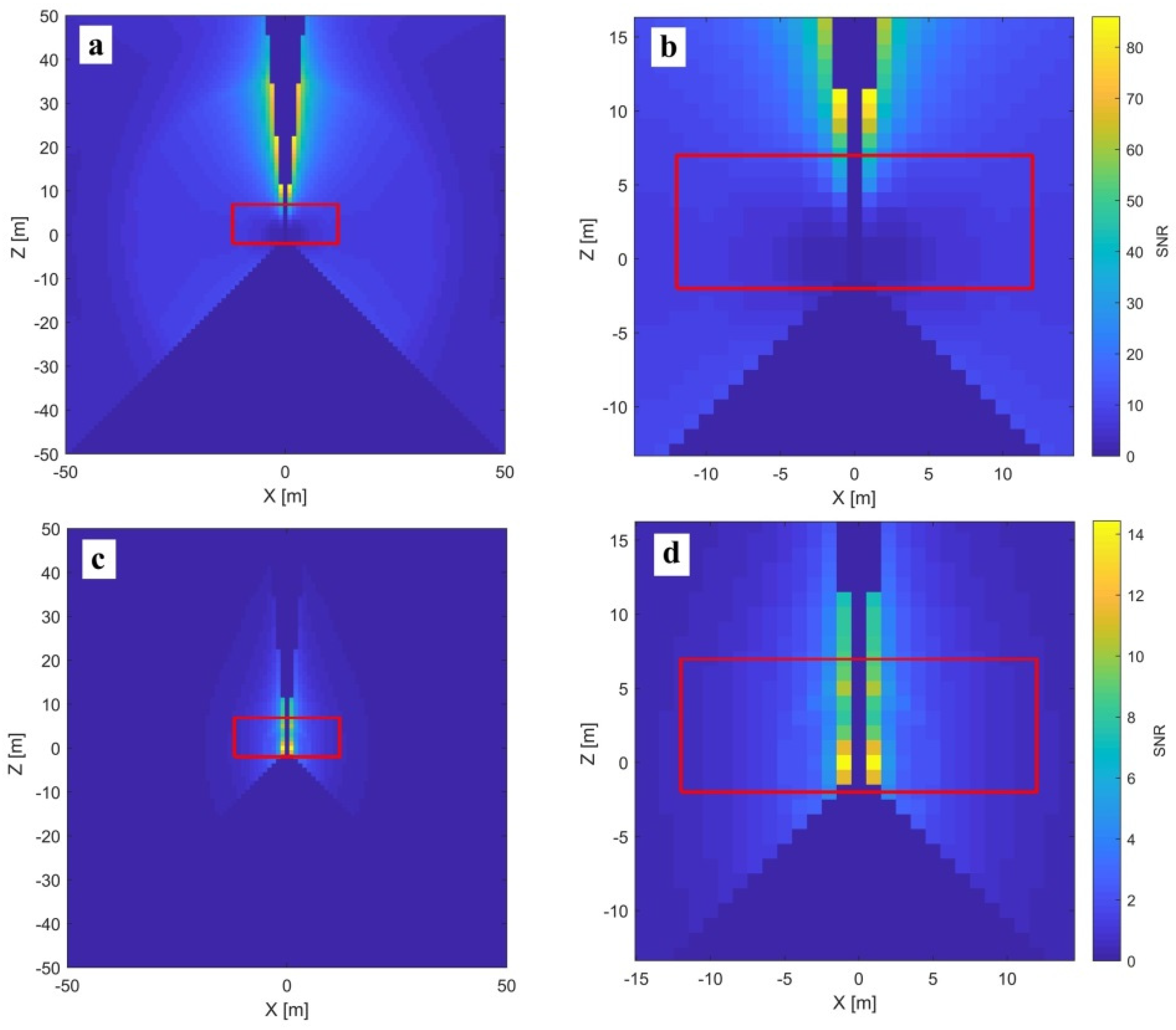
3.1.1. $x_2$—Horizontal Axis Offset

Horizontal axis offset ($x_2$) impacts the range and the vertical angle measurements (Equations (2) and (4)). In both cases, it is a two-face sensitive parameter. However, in the case of the vertical angles, it is perfectly coupled with the horizontal beam offset ($x_{1n}$) due to its identical functional description. Hence, its impact on the vertical angles will be discussed in one of the following sections as $x_{1n+2}$. Here, we concentrate on $x_2$ as a stand-alone parameter and its impact on the range measurements.

As the x₂ is an offset parameter, the impact of the misalignment (signal) is constant with the distance and changes only with respect to the vertical angle. From Figure 7, it is apparent that the highest SNR is achieved in the horizontal plane of the instrument, where the signal is the highest ($x·\sin {90}^{°}=x$) and decreases with the sine function both in the directions of the zenith and nadir. Based on the stochastic model in Figure 3, the range measurement noise grows with the distance, except for an increased value in the proximity of the instrument (the first few meters). Additionally, it is advisable to avoid distances smaller than three meters due to unmodeled near-field systematic errors (Section 2.4). Hence, this parameter is the best estimated by the two-face measurements of a target in the instrument’s horizon at a distance of approximately three meters. With this measurement configuration, no other parameter impacts the two-face difference in the range direction, and the $x_2$ estimate is completely de-coupled from the other CPs.

The red rectangle (Figure 7) represents the dimensional limitations of one vertical cross-section of the facility used in the empirical experiment (25 m × 9 m). In this particular case, it poses no constraint, and the most sensitive measurement configuration can be easily implemented within the facility.

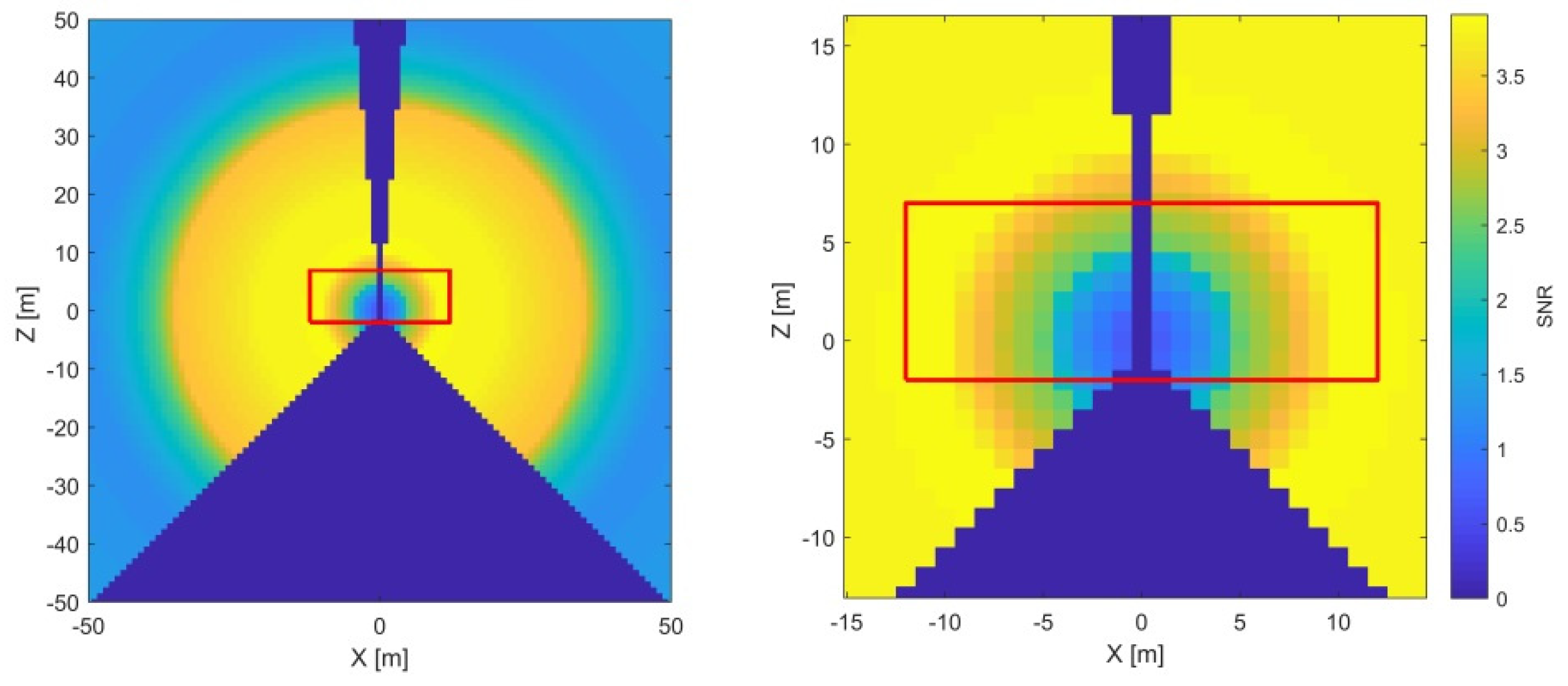
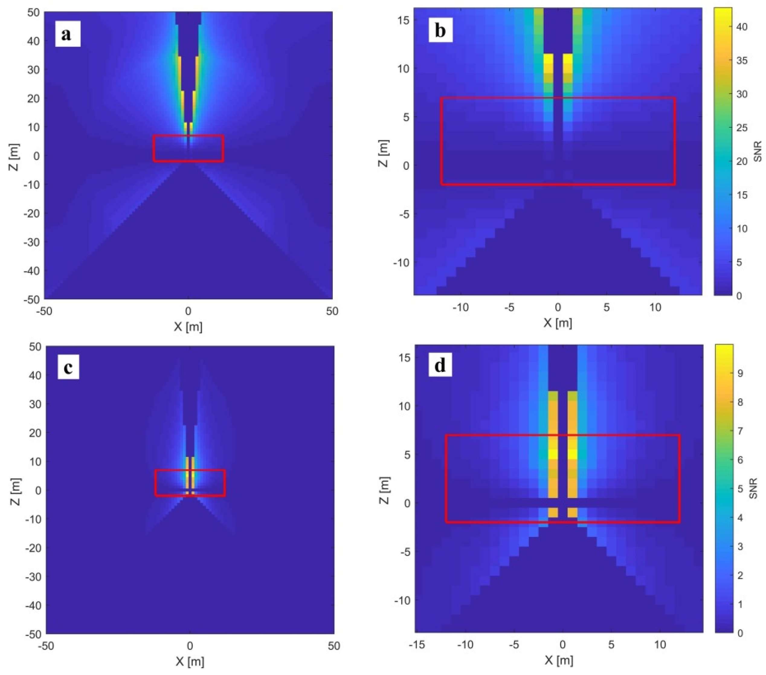
3.1.2. $x_4$—Vertical Index Offset

The vertical index offset ($x_4$) causes a systematic error in vertical angles (Equation (4)). The related point displacement (signal) grows proportionally with the distance. Additionally, the signal is constant with respect to both horizontal and vertical angle measurements. The corresponding SNR analysis is presented in Figure 8 (left).

The only misalignments that additionally influence the two-face differences of the vertical angles change with the cosine of the vertical angles ($x_{5n}$ and $x_{1n+2}$, Equation (4)). Hence, their signal is zero in the instrument’s horizon ($\cos {\theta }_{{90}^{°}/{270}^{°}}=0$) and, here, the $x_4$ estimate is completely de-coupled from the other CPs. The measurement’s uncertainty in the direction of the vertical angles is the lowest at distances from 10 to 20 m (Figure 3), and, consequently, the SNR ratio is the highest. Hence, this parameter is best estimated by two-face measurements of a target in the instrument’s horizon at a 10 to 20 m distance. As in the previous case, the physical limitations of our facility do not pose a problem in achieving this measurement configuration (Figure 8, right).

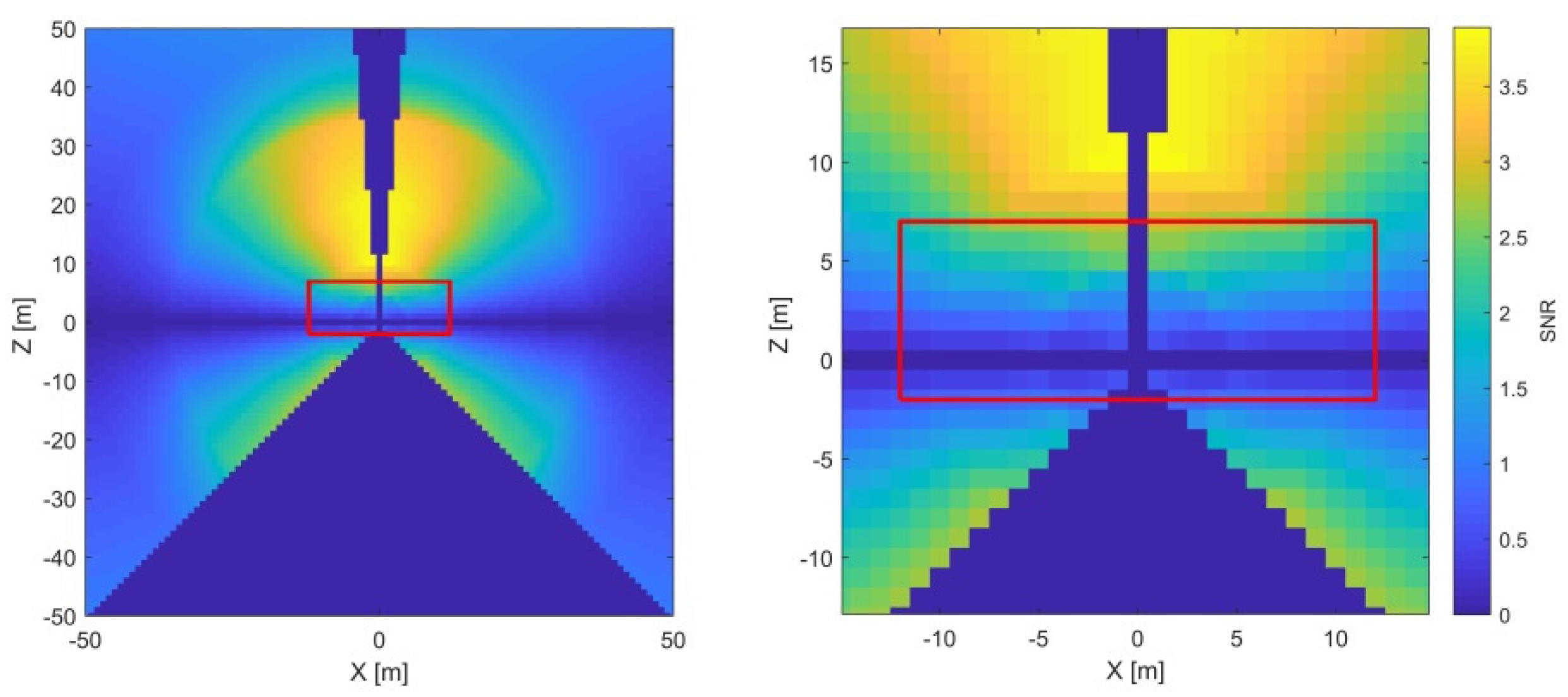
3.1.3. $x_{5n}$—Horizontal Beam Tilt and $x_{1n+2}$—Horizontal Beam and Horizontal Axis Offsets

The horizontal beam tilt ($x_{5n}$) impacts the vertical angle measurements (Equation (4)). Its signal proportionally grows with the distance and decreases with the cosine of the vertical angle. Hence, due to the unmeasurable conical area underneath the instrument, its signal is the highest in the proximity of the local zenith (Figure 9, left). In this constellation, its signal is coupled with the signal of $x_4$ (overlapping yellow regions in Figure 8 and Figure 9). Therefore, to estimate $x_{5n}$, it is mandatory to have at least one additional target at the instrument’s horizon to estimate and eliminate the effect of $x_4$. In the ideal case, this parameter is best estimated by observing a target at a distance of 10 to 20 m in the zenith direction (the highest SNR). However, this constellation is hard to achieve in reality due to the usual limitations of both indoor and outdoor facilities. Hence, there is often a compromise between the length and the inclination (slope) of the line-of-sight. In general, for indoor calibration fields, the SNR is directly dependent on the ceiling height and is expected to be sub-optimal (Figure 9, right). Hence, the target should be placed as high as possible, and preferably more than one target should be used to improve the quality of the estimated parameter. This fact has to be considered during the selection of the appropriate calibration facility, where facilities with higher ceilings are preferred.

One target near the zenith is insufficient for the unbiased estimation of $x_{5n}$. Namely, this constellation leads to the perfect coupling with the parameter $x_{1n+2}$, which shares an almost identical functional description (Equation (4)).

Parameter $x_{1n+2}$ combines the effect of the horizontal beam and the horizontal axis offset, and it impacts the vertical angle measurements. Its signal is constant with the distance and decreases with the cosine of the vertical angle. Based on the SNR analysis in Figure 10 (left), the best constellation is realized by placing a target as close as possible to the zenith in the proximity to the scanner (without disregarding the near field considerations given in Section 2.4). In general, in order to de-couple $x_{1n+2}$ and $x_{5n}$, it is necessary to have at least two elevated targets at different distances, with respect to the instrument. The bigger the difference in distances between these two targets, the better the parameter de-coupling.

Due to the highest SNR, in the best-case scenario, both targets are placed in the proximity of the local zenith at different distances (10–20 and 3 m). Unfortunately, this is hard to implement in a typical indoor environment. An alternative possibility for a good measurement configuration for estimating $x_{1n+2}$ is placing a target on the floor next to the instrument, as close as possible to the nadir direction (Figure 10, right). However, for this alternative, the near field problems should be resolved.

3.1.4. $x_6$—Mirror Tilt and $x_3$—Mirror Offset

The mirror tilt ($x_6$) and offset ($x_3$) influence the horizontal angle measurements with the signal increasing with the reciprocal sine of the vertical angles and reaching infinity in the zenith (Equation (3)). The difference between them is that the signal of the $x_6$ increases according to distance with respect to the instrument (Figure 11a,b), while the signal of $x_3$ is constant (Figure 11c,d). To estimate these parameters separately, at least two targets at different distances are necessary.

In general, for both parameters, similar conclusions apply, like for the previous pair of CPs ($x_{5n}$ and $x_{1n+2}$). The main difference is that these parameters can be estimated in the instrument’s local horizon ($\frac{x_3}{\sin {90}^{°}/{270}^{°}}=x_3$), which produces some important advantages and one disadvantage. The advantages are that the parameters in this constellation are de-coupled from the rest of the two-face sensitive parameters, influencing the horizontal angle measurements ($x_{5z-7}$ and $x_{1z}$); the target mounting is simple; and achieving longer distances is manageable in the indoor facilities (Figure 11c). The disadvantage is that the SNR ratio is comparably low with respect to the maximal achievable value. However, even with this reduced SNR, the parameters can be estimated with uncertainty below the single point measurement noise. Therefore, considering all the advantages and disadvantages, a cost-efficient measurement configuration consists of two targets placed in the local horizon, one in proximity to the scanner (e.g., at 3 m) and one at a distance of 10–20 m.

3.1.5. $x_{5z-7}$—Vertical Beam Tilt and Horizontal Axis Tilt and $x_{1z}$—Vertical Beam Offset

The parameters $x_{5z-7}$ and $x_3$ are similar to the parameters explained in the previous section. They are the corresponding tilt and offset parameters that cannot be estimated separately. These parameters impact the horizontal angle measurements, and their signal grows with the reciprocal tangents of the vertical angle. Moreover, they have no signal in the instrument’s horizon ($\frac{x_{5z-7}}{\tan {90}^{°}/{270}^{°}}=0$). Above the horizontal plane, they are perfectly coupled with the parameters $x_6$ and $x_3$. Hence, the latter two parameters need to be estimated a priori, or at least two targets in the horizontal plane are additionally required when considering the measurement configuration for the $x_{5z-7}$ and $x_{1z}$.

The highest SNR for both parameters is achieved near the local zenith, where, for the tilt parameter, it is at a 10–20 m distance from the scanner (or maximum ceiling height indoors), while, for the other, it is in the scanner’s proximity. Again, there is an alternative for the tilt parameter in sense of placing the target on the floor as close as possible to the instrument (Figure 12d), if the near-field problems indicated in Section 2.4 are resolved.

It should be noted that although the parameters $x_{5z-7}$ and $x_{1z}$ are perfectly coupled with the parameters $x_6$ and $x_3$ when all targets are placed above the instrument’s horizon, they are decoupled if the targets are evenly distributed above and below the horizon. Namely, the parameters $x_{5z-7}$ and $x_{1z}$ retain the same sign both above and below due to the tangent function, while the parameters $x_6$ and $x_3$ change the sign. This makes both groups separable. However, this brings little to no benefit for the estimation of tilt parameters in the typical indoor environment. Namely, the preferred distances of 10 to 20 m from the scanner are impossible to achieve below the horizon without using some highly elevated platform. This leads to a low SNR for all target constellations underneath the instrument’s horizon (Figure 11b and Figure 12b).

3.2. Sensitivity Analysis of the Length-Consistency Tests

There is one general point that needs to be considered for length-consistency tests—the angle between the line-of-sight and the test-length is important. In the case of angular measurements, if the line-of-sight forms a right angle with the test-length, the full impact of the misalignment will cause length deformation, so the signal will be high. In contrast, if the test-length and the line-of-sight are parallel, the complete impact of the misalignment will cause length rotation, and the signal will be null. The case is opposite for the range measurements. This phenomenon stems from the simple geometrical relationships of the observed quantities and will be used as a main guiding principle in deriving and understanding the most sensitive length-tests. As in the case of the two-face differences, we additionally need to aim for the highest influence of the misalignments with respect to range and angular measurements, as well as the minimum measurement uncertainty with respect to the stochastic model (Section 2.4).

As it was previously stated, our goal is to observe two targets from two TLS stations, where from one of them the length is maximally deformed, and from the other, it is minimally deformed. In the optimal case, the observations from the first station would cause the length deformation (e.g., extension), while they would cause no deformation from the second station or a deformation with the opposite sign (e.g., contraction). Therefore, to be able to derive the most sensitive configuration for both cases, we use the signed signal for the SNR analysis in this section. The positive sign corresponds to the length extension, while the negative one corresponds to the length contraction. The most sensitive length-consistency tests for the parameters not sensitive to two-face differences (Figure 6) are derived in the following sections.

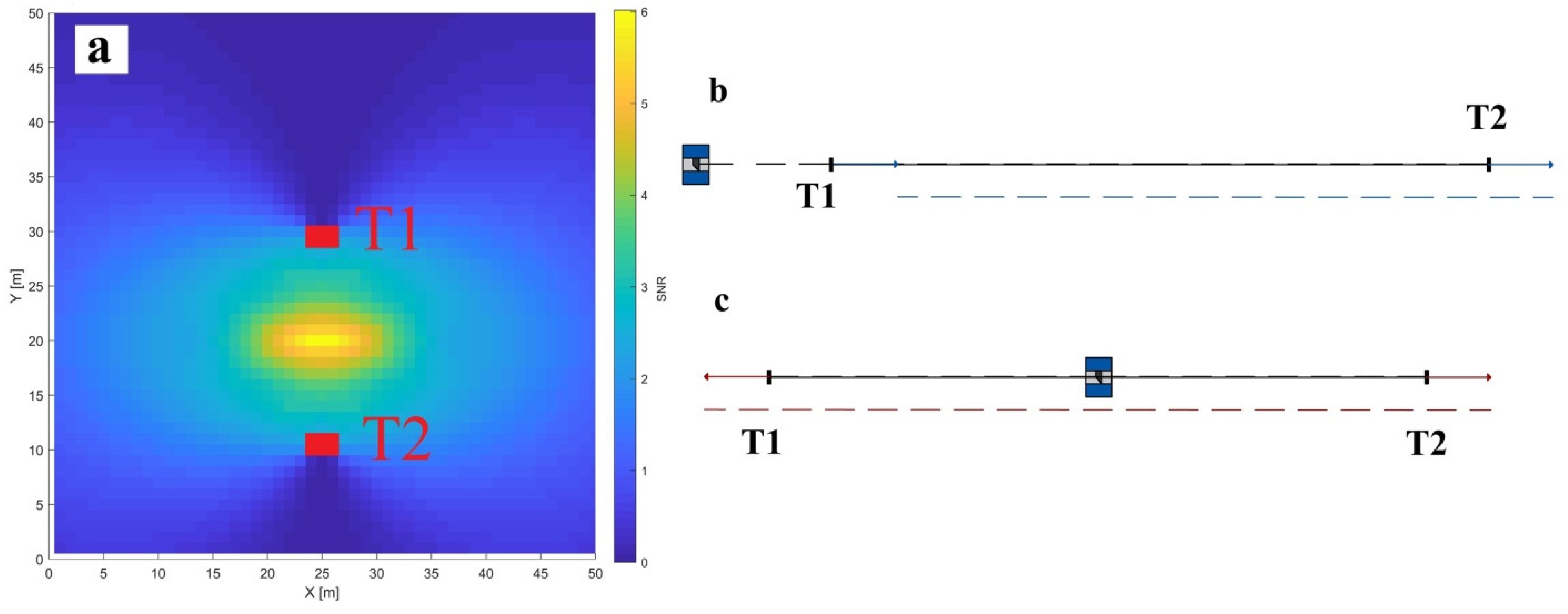
3.2.1. $x_{10}$—Rangefinder Offset

As the impact of the rangefinder offset ($x_{10}$) is constant with respect to the range measurements, the relative distance between two targets used for the length test is of less importance. Hence, we selected a constant distance of 20 m between targets T1 and T2, and we simulated all possible instrument positions with respect to the test-length $\overline{T1T2}$. Additionally, as this parameter is invariant to the vertical angles, we reduced the sensitivity analysis to the 2D analysis in the instrument’s local horizon (Figure 13a). In this simulation, the origin of the 2D coordinate system is arbitrarily defined in space, and every pixel in the image represents the instrument’s position with respect to the observed targets (T1 and T2).

The highest SNR is realized when the instrument is placed in-line and in-between the targets where the whole impact of the misalignment is transferred to a length change (extension). In contrast, the lowest SNR is realized when it is placed in-line and aside from the targets, where the whole misalignment impact causes length translation in space. These two positions together form the inside-out test (Figure 13c as inside and Figure 13b as outside), which is the most sensitive selection of target–to–TLS positions for the estimation of the rangefinder offset and is often used for the calibration of laser trackers [53]. This test has the unavoidable problem that one of the targets, i.e., one point in space, needs to be observed from two sides (Figure 13—target T1). This issue poses difficulties for adequate target construction that would allow the accurate transfer of measurements from both sides and guarantee sufficient accuracy for the calibration.

If adequate targets are not available, the best alternative based on this sensitivity analysis is to place the instrument once in the middle, in-line with targets, and once in the middle (equidistant), but away from both targets (e.g., in Figure 13a: X = 0, Y = 20). Then, in the latter case, most of the misalignment’s impact will be transferred to the translation of the length test in space. It is worth noting that the target center in the direction of range measurements is best estimated at shorter distances from the instrument (Figure 3), if we disregard the near-field problems. Hence, it is beneficial to keep the overall test length dimensions smaller.

3.2.2. $x_{1\mathrm{n}}$—Horizontal Beam Offset

Horizontal beam offset ($x_{1\mathrm{n}}$), as a stand-alone parameter (without perfect coupling with $x_2$), impacts the horizontal angles and is not estimable using two-face differences. Therefore, the length consistency test is discussed in detail. Alternatively, $x_{1\mathrm{n}}$ can be indirectly estimated by subtracting the parameter $x_2$ (Equation (2)) from $x_{1\mathrm{n}+2}$ (Equation (4)) if both CPs are estimated with sufficient accuracy [23].

The signal of $x_{1\mathrm{n}}$ has a constant value with respect to all TLS measurements, which allows us to simulate a length-test with fixed dimensions in the instrument’s horizon, in the same manner as it was realized for $x_{10}$ (Figure 13a and Figure 14a).

It is prominent that the most sensitive positions are next to the test-length $\overline{T1T2}$, as close as possible to one of the targets, with the line-of-sight aiming at the nearby target that is perpendicular to the test-length. On the contrary, most insensitive positions are in-line and in between the targets. Namely, from the latter position, the impact of $x_{1\mathrm{n}}$ is completely transferred to the length rotation (Figure 14b). It is observable that the impact of $x_{1\mathrm{n}}$ changes its sign when the instrument is placed from the right (Figure 14c), causing length extension, and when it is placed from the left (Figure 14d), it causes length contraction. Hence, for the self-calibration, any combination of measurement configurations, b and c (or b and d), or a combination of c and d, can be used (Figure 14b–d). The latter combination doubled the value of the SNR. Thus, it is more sensitive. However, it also requires a special target design allowing the measurement of the same point in space from both sides, as discussed for $x_{10}$.

The closer we place the instrument to the target, the more sensitive the test is. However, the near-field problems should not be overlooked. The simple possibility to find a compromise in this particular case is to transfer this length-test from a 2D to 3D case. Namely, if we place one of the targets highly above the TLS, e.g., on the ceiling near the zenith, the distance to the target will be sufficiently long while the test sensitivity will remain the same. This holds true because $x_{1\mathrm{n}}$ is invariant to the vertical angle measurements (i.e., the target’s height), and, therefore, only the 2D projection of this 3D test-length is relevant.

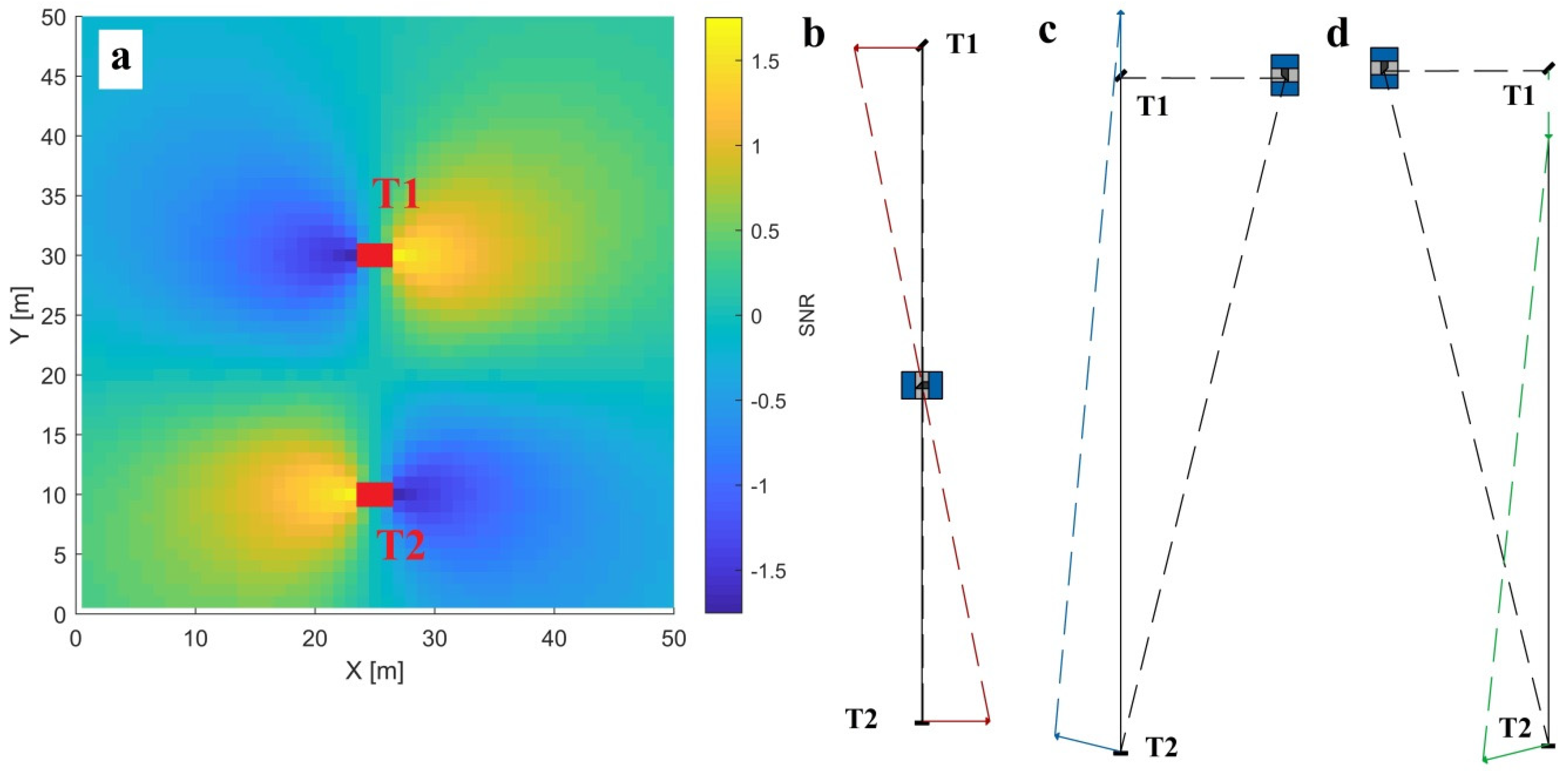
3.2.3. $x_{5\mathrm{z}}$—Vertical Beam Tilt

The impact of vertical beam tilt ($x_{5\mathrm{z}}$) on the horizontal angle measurements is perfectly coupled with $x_7$ and, therefore, it is treated as a separate CP—$x_{5\mathrm{z}+7}$ (Equation (3)). As a stand-alone CP, vertical beam tilt impacts the vertical angles (Equation (4)) and its impact grows proportionally with the distance and sine of the vertical angles and reaches the highest value at the instrument’s horizon. Vertical beam tilt is highly correlated with $x_{1\mathrm{z}}$, which shares a similar functional connection with the vertical angles (Equation (4)). Therefore, it is necessary to estimate $x_{1\mathrm{z}}$ either a priori or at the same time, e.g., by utilizing the two-face differences described in Section 3.1.5.

The sensitivity analysis can be reduced to a 2D problem in a vertical plane passing through the origin of the TLS local coordinate system (as in Figure 7, Figure 8, Figure 9, Figure 10, Figure 11 and Figure 12). Namely, this parameter is invariant to horizontal angles and causes target displacement within the latter vertical plane. Hence, it will achieve the highest signal if both targets and the TLS are within one vertical plane. If the test length is placed further away from the TLS, i.e., in a vertical plane not passing through the origin of the local TLS coordinate system, the impact of $x_{5\mathrm{z}}$ will be transferred to a length translation and not the length change. We will demonstrate this in the following paragraphs based on an example.

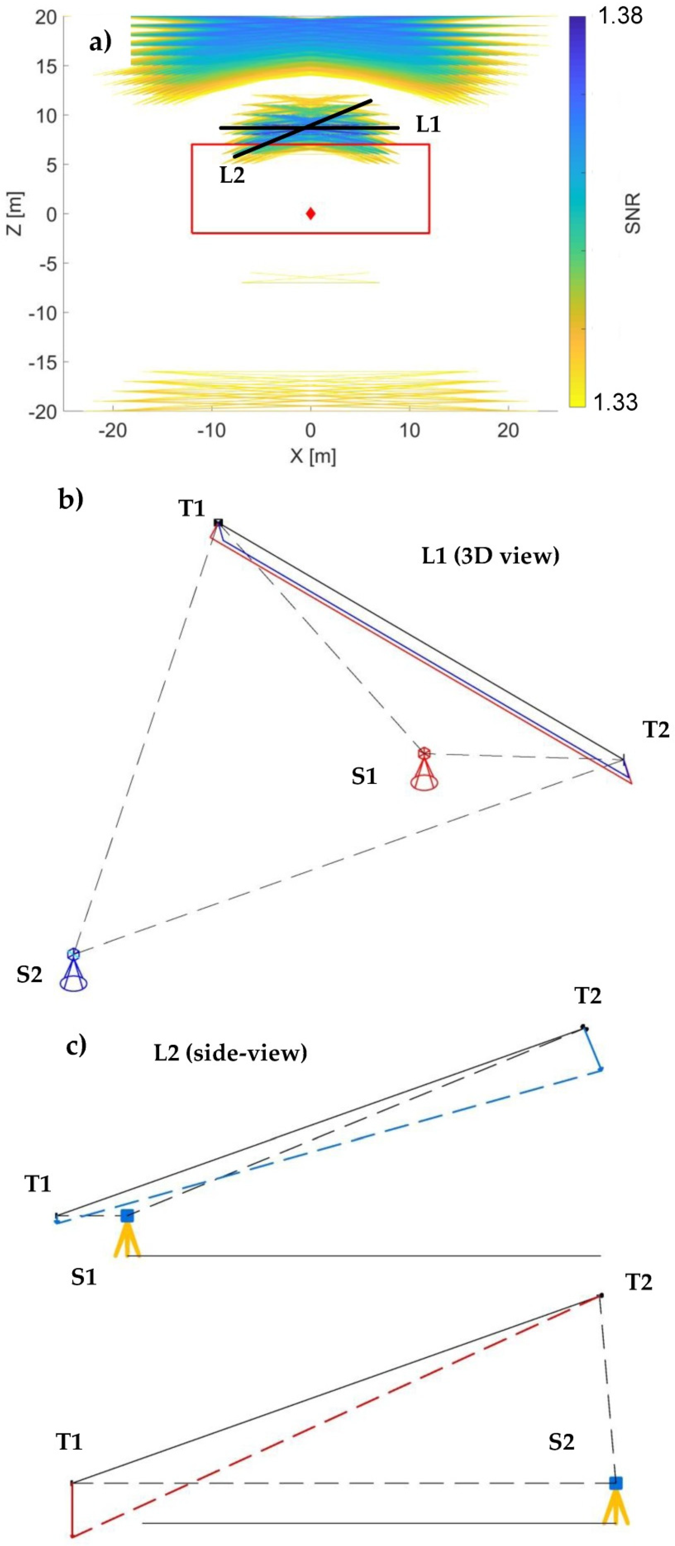
We simulated all possible positions for the length-test, as a combination of two targets (T1 and T2) within the scanners field-of-view. As the effective visualization of all theoretical solutions is not possible, in Figure 15a we present only 1% of the solutions with the highest SNR.

The instrument’s location is presented with the red rhomboid, the red rectangle represents the spatial limitations of the indoor facility used in the empirical experiment, and the colored lines represent the sensitive positions of the test-lengths, with blue as the most sensitive and yellow as the least sensitive (from the most sensitive 1%). The first apparent point is that all of the sensitive positions are quite similar. From all presented possibilities, we highlighted the two most different ones (black lines L1 and L2), as the others are generally somewhere in between.

The first and the most sensitive position is if we place the length-test symmetrically above the scanner so that the TLS–to–target distances are approximately 10 m and the vertical angles to the targets are in between 50–60°/300°-310° (Figure 15a, line L1). The latter condition is important because, if the vertical angles are closer to 0°/360°, the signal of $x_{5\mathrm{z}}$ will be lower (due to the sine function). Additionally, if the targets are placed close to the instrument’s horizon (90°/270°), $x_{5\mathrm{z}}$ will cause a translation of the test-length in the z-axis direction instead of the length change. A similar sensitivity is achieved for different elevations of the length-test and changes only with respect to the expected noise of the angular measurements (Section 2.4).

The second sensitive measurement configuration is when the length-test is realized as a vertical diagonal in space (Figure 15a, line L2), so that one point is placed directly above the instrument (near the zenith) and the other point is placed towards the instrument’s horizon.

If we relate the maximum achievable value of the SNR for $x_{5\mathrm{z}}$ with other angular CPs (Figure 8, Figure 9, Figure 10b and Figure 12b), it is comparably low. Hence, successful estimation of $x_{5\mathrm{z}}$ poses a special challenge. Therefore, we explain, in detail, both realizations (L1 and L2) of the most sensitive length-consistency tests (Figure 15b,c).

Length Consistency Test L1

Figure 15b presents the realization of this length consistency test in 3D, from both the most (S1) and the least (S2) sensitive scanner stations, with respect to the test-length $\overline{T1T2}$. From station S1, the targets are symmetrically placed above the scanner based on the most sensitive position indicated in Figure 15a. The impact of the parameter causes the length extension indicated with a red line. From Figure 15a, it is observable that the main constraint with respect to the sensitivity of this test-length in typical indoor environments is the ceiling height. Hence, the test should be realized as high as possible.

To obtain a reference value for $\overline{T1T2}$ (with the length minimally deformed), the instrument should be placed away of the test-length (S2). With this constellation, $x_{5\mathrm{z}}$ mostly causes a length translation in the downwards direction (indicated in blue). The TLS should not be placed too far off $\overline{T1T2}$, as this leads to a higher measurement uncertainty and, hence, the uncertainty of estimating the reference value of $\overline{T1T2}$.

Length Consistency Test L2

Figure 15c presents this length consistency test in 2D, both for the most (S2) and the least (S1) sensitive TLS–to–target configuration. There are two important guidelines to increase the sensitivity of this test.

One guideline is that the test-length needs to be placed as much as possible perpendicular to the line-of-sight when observing to the target T1 from the station S2. In this case, the full impact of $x_{5\mathrm{z}}$ will cause a length change. The other guideline is that the target T1 needs to be placed far from the instrument on station S2, because the impact grows linearly with the distance, without disregarding the increase of the measurement noise with the distance.

Both guidelines are directly dependent on the maximum achievable height of target T2. Hence, in the case of the indoor calibration, they depend on the ceiling height. Namely, if target T1 is placed further away from the scanner, the elevation of target T2 has to be adjusted to have perpendicular line-of-sight with respect to the test-length. Otherwise, the impact of $x_{5\mathrm{z}}$ will increase due to the longer TLS–to–target distance, but at the same time, it will decrease due to worse line-of-sight vs. test-length configuration. Hence, without increasing the elevation of target T2, no gain with respect to SNR can be achieved.

To retrieve the non-deformed reference for $\overline{T1T2}$, the TLS needs to be placed as close as possible to target T1 (Figure 15c, S1). Here, T1 is minimally displaced due to a small TLS–to–target distance, while the displacement of the target T2 causes only the rotation of $\overline{T1T2}$ in space.

Because, in general case, it is easier to assemble the second measurement configuration (L2), this configuration is used as a part of the manufacturer’s on-site calibration approach—Leica Check and Adjust [54]. As both presented length-tests exhibit lower SNR in comparison to the other tests, several repetitions are recommended for a successful parameter estimate.

3.3. Discussion of Sensitivity Analysis

Apart from the most sensitive measurement configurations for estimating each CP, there are several take-away messages that should be highlighted.

The main point is that the dimensions of the facility used for the TLS calibration are important, especially the ceiling height. The perfect calibration facility would have a cubical shape with dimensions between 20 × 20 × 20 and 10 × 10 × 10 m. Rooms with notably smaller dimensions can hardly be used for cost-efficient TLS calibration (cost-efficient in a sense of a reduced target number). Namely, they hinder using sufficiently sensitive measurement configurations, and they do not allow adequate dispersion of targets necessary to de-couple functionally similar tilt and offset parameters. Hence, considerably smaller facilities can only be used for the full-blown target-based self-calibration with dozens of targets, as was demonstrated in multiple experiments in the past.

In most cases of the indoor TLS calibration, the limiting factor is the ceiling height, and this should be the main guideline when selecting an appropriate facility. In order to increase the sensitivity in a room with limited dimensions, two modifications can be applied—short tripods, allowing the instrument placement only several centimeters above the ground, and mirrors placed on the ceiling, artificially extending the steep lines-of-sight, as already suggested in [41].

Facilities with larger dimensions than suggested can be utilized. However, they would not provide additional benefits in the sense of improved CP estimates. The conducted sensitivity analysis reveals that it is not necessary to observe targets evenly distributed within the full instrument’s field of view and with the full working range of 1–100 m. The benefit of targets below the instrument’s horizon, as well as at distances smaller than 3 m and higher than 20 m, is minimal. This directly stems from the uncertainty of estimated target centers (Figure 3). Additionally, all sensitive measurement configurations can be realized by placing targets within one vertical and one horizontal plane. This point can be used to significantly reduce the computational problem of the optimization algorithms when the optimal solutions for different instruments and specific facilities are searched.

Although the conducted sensitivity analysis aims at target-based self-calibration, the derived sensitive measurement configurations can be also considered for other state-of-the-art calibration methods (Section 1). The uncertainty of the target centers in the range direction (Figure 3), and, hence, the positions with the highest SNR can be directly transferred to the plane-based self-calibration approach. For example, in order to estimate the parameter $x_2$ (Section 3.1.1), the target from the sensitivity analysis can simply be substituted with any planar surface, and the results will be equivalent. Similarly, other sensitive measurement configurations can be transferred to the instrument-to-cylinder or –plane configurations. For example, the CP $x_{5z}$ (Section 3.1.5) could also be estimated according to the measurement configuration presented in Figure 15c, if targets T1 and T2 are substituted with cylinders perpendicular to the line connecting stations S1 and S2. The only difference between the targets and other geometric primitives lies in degrees of freedom (DoF), i.e., the number of sensitive directions. Namely, the movement of the target center can be detected in any direction (3 DoF), while the movement of the plane can only be detected in the direction of the plane normal (1 DoF), and the movement of the cylinder can be detected in all directions except in the direction of the cylinder’s axis (2 DoF).

The conducted sensitivity analysis additionally proved that all CPs can be estimated using only TLS measurements without reference values realized with the instrument of superior accuracy, which only confirms the proceeding studies on the topic.

The derived sensitive measurement configurations can be used to calibrate all TLSs of a panoramic type described in Section 2.1. The only problem could be software limitations because some manufacturers do not enable the two-face measurements principle by default. To acquire the most sensitive measurement configuration for a specific instrument, the stochastic model used to calculate the noise level in the SNR analysis should be adjusted accordingly. This can lead to somewhat different optimal TLS-to-target(s) distances. However, the recommended measurement configurations will remain the same. The conducted sensitivity analysis is not directly transferable to hybrid and camera type TLSs, as they generally have different measurement mechanisms and, hence, different misalignments that need to be modeled. Additionally, their field-of-view is different, which introduces different measurement limitations.

The main deficiency of the conducted sensitivity analysis is that it does not address the problems of calibrating the angular encoders, as well as the comprehensive calibration of the rangefinder. These additional calibration steps are necessary if the instruments do not use multiple reading heads and if there are additional rangefinder related systematic errors influencing measurements (e.g., cyclic and scale error). In such cases, parameter estimates based on the presented measurement configurations are still valid, but not necessarily unbiased.

4. Minimal Measurement Geometry

In this section, we demonstrate how the presented sensitivity analysis can be used for designing the calibration field. The intention of this section is not to derive the optimal calibration field implementation for the instrument under investigation. This will be a focus of further study. Rather, the main aim is to present how calibration field complexity (the number of targets and scanner stations) can be effectively reduced if the sensitivity of estimating individual calibration parameters is considered. Section 4.1 introduces a design with minimal measurement geometry; Section 4.2 presents a simulation experiment that proves the theoretical possibility of the suggested minimal geometry to reveal all of the relevant CPs, Section 4.3 concentrates on an empirical experiment analyzing the applicability of the proposed geometry in reality, and Section 4.4 shortly underlines the main takeaway message of the presented results.

4.1. Design of Minimal Measurement Geometry

Based on the sensitivity analysis, we derived the minimal number of targets and scanner stations necessary for revealing all calibration parameters from Equations (2)–(4). Namely, we need:

• Two-face differences for 1 target on the instrument’s horizon at a short distance to estimate $x_2$ and $x_3$ and 1 target at a long distance to estimate $x_4$ and $x_6$;
• Two-face differences for 1 elevated target at a short distance to estimate $x_{1n+2}$ and $x_{1z}$ and 1 elevated target at a long distance to estimate $x_{5n}$ and $x_{5z+7}$;
• Length consistency tests for $x_{1n}$, $x_{5z}$, and $x_{10}$.

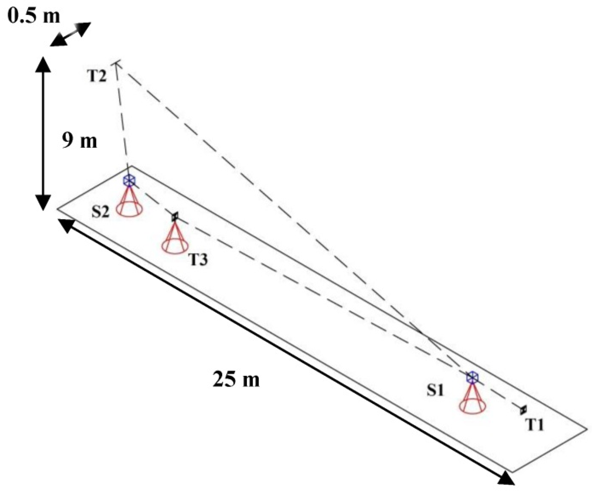
The minimal measurement geometry that incorporates all the above-mentioned criteria is presented in Figure 16. We simulated the target and scanner station locations based on the dimensions of the facility that is used in the empirical experiment in Section 4.2.

Only three targets measured from two stations using two-face measurements are sufficient if the targets are placed on the predefined locations. Target T1 and scanner stations S1 and S2 are approximately within 1 line and at the same height. Target T3 is placed slightly aside, only enough to allow clear line-of-sight between S2 and T1. Finally, target T2 is placed 0.5 m aside from the line S1–S2–T1 on the highest possible elevation. The shortest lines-of-sight are always higher than 3 m, while the longest ones are lower than 20 m.

Target T1 fulfils the requirements of the first bullet point (a short distance from S1 and a long distance from S2). Target T2 fulfils the requirements of the second bullet point (a short distance from S2 and a long distance from S1). The length $\overline{T1T2}$ is simultaneously sensitive for estimating $x_{1n}$ and $x_{5z}$. Namely, as T2 is placed next to the scanner station S2, from this position, this setup imitates the measurement configuration from Figure 14c, while from S1, it imitates the configuration from Figure 14b. Additionally, the achieved measurement configuration allows an estimation of $x_{5z}$ based on the length-consistency test described in Figure 15c. The inside-out test for estimating $x_{10}$ requires an additional target (T3) in-between the scanner stations S1 and S2 (Figure 13a,b). If the rangefinder offset is estimated a priori, only targets T1 and T2 would be necessary for revealing all of the remaining calibration parameters.

4.2. Simulation Experiment

The values of the simulated mechanical misalignments are given in

Table 2. The results of the simulation experiment: CP values (simulated and estimated) and standard deviation.

Par.	${\mathit{x}}_{\mathit{t}\mathit{r}\mathit{u}\mathit{e}}$	$\widehat{\mathit{x}}$	${\mathit{\sigma }}_{\mathit{x}}$
${\mathit{x}}_{\mathbf{10}}$ [mm]	−2.00	−1.98	0.04
${\mathit{x}}_{\mathbf{2}}$ [mm]	−0.20	−0.23	0.02
${\mathit{x}}_{\mathbf{1}\mathbf{z}}$ [mm]	−0.20	−0.24	0.03
${\mathit{x}}_{\mathbf{3}}$ [mm]	−0.20	−0.20	0.01
${\mathit{x}}_{\mathbf{5}\mathbf{z}+\mathbf{7}} \left[″\right]$	−16.00	−14.74	1.04
${\mathit{x}}_{\mathbf{6}}$$\left[″\right]$	−8.00	−7.99	0.09
${\mathit{x}}_{\mathbf{1}n}$ [mm]	−0.20	−0.21	0.01
${\mathit{x}}_{\mathbf{4}}$$\left[″\right]$	−8.00	−8.06	0.13
${\mathit{x}}_{\mathbf{5}\mathbf{n}}\left[″\right]$	−8.00	−8.48	1.05
${\mathit{x}}_{\mathbf{5}z}$$\left[″\right]$	−8.00	−7.89	0.62
${\mathit{x}}_{\mathbf{1}n+\mathbf{2}}$ [mm]	−0.40	−0.36	0.03

. We selected these magnitudes as realistic ones based on the experience from previous experiments [23]. The measurements are simulated with measurement noise based on the stochastic model in Section 2.4. We additionally analyzed the standard deviations of the estimated CPs. We included the compensator measurements, as they are used in the empirical experiment. The adjustment is realized based on the functional and stochastic models presented in Section 2.3 and Section 2.4.

The estimated CPs fit very closely to the true values without any bias. All of the offset parameters are estimated with an accuracy of several tenths of the millimeter. In the case of the tilt parameters, the ones that are estimated using the targets on the horizon are estimated with a standard deviation of 0.1” ($x_6$ and $x_3$), while the rest ($x_{5z}$, $x_{5z-7}$, and $x_{5n}$) are estimated with a standard deviation of within 1”.

The correlations between CPs and other unknowns are not presented and analyzed in detail. They are, as expected, extremely high (nearly 100% in most cases), as much more complex measurement geometry is necessary to decouple such a high number of functionally similar CPs. To conclude, this simulation experiment confirmed that it is theoretically possible to estimate all relevant CPs with a minimum of three targets observed from two scanner stations.

4.3. Empirical Experiments

The measurement setup used in the empirical experiment is described in Section 4.3.1. The calibration adjustment was conducted twice. The first time, we tried to estimate all relevant CPs to have a direct comparison with the simulation experiment. In Section 4.3.2, we present the results and discuss them with respect to the TLS test-fields defined in ISO (International Organization for Standardization) norms [32]. Thereafter, we discuss the relation of the derived minimal measurement geometry with the manufacturer’s in-situ calibration approach (Leica Check and Adjust [54]), which aims at estimating a selected subset of CPs. The results of this partial TLS calibration are given in Section 4.3.3, together with the corresponding discussion.

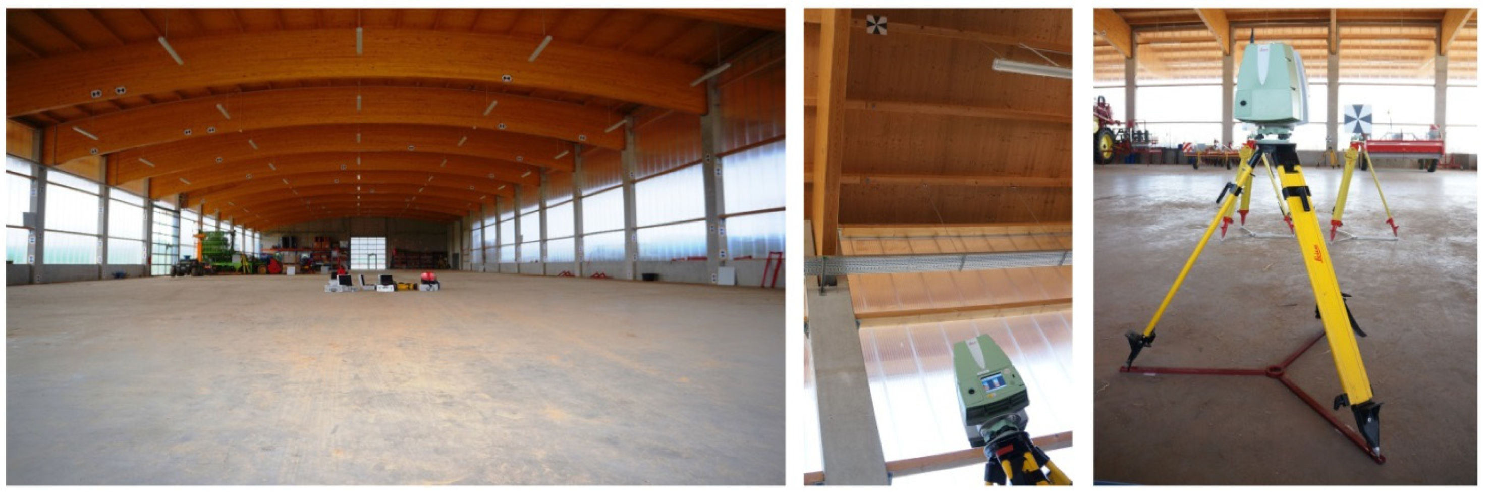
4.3.1. Measurement Setup

We implemented the measurement configuration from Figure 16 in the facility that we have at hand for the calibration of TLSs with approximate dimensions of 33 × 75 × 9 m (Figure 17). The targets used were black and white BOTA8 targets, which assure high precision of the target center estimation [46]. The target centers were estimated using the algorithm based on the template matching described by Janßen et al. 2019 [46]. From each scanner station, two-face measurements were made and the compensator was turned on. We selected the second highest measurement resolution, as it was demonstrated that there was no loss in the target center’s precision with a four times shorter measurement time [24]. Additionally, a quality level 1, without range measurement averaging, was used [55].

The described measurements were repeated four times within two days (two repetitions per day). Before each calibration attempt, the instrument was warmed-up for one hour. Each of the repetitions required approximately 1 h. During the measurements, the atmospheric conditions were monitored and were stable during each day (1st day: 29 °C, 990 hPa, 40% humidity; 2nd day: 27.5 °C, 991 hPa, 55% humidity). As all range measurements were short (<20 m), no atmospheric correction was used.

For estimating the rangefinder offset ($x_{10}$), it is necessary to observe a single target from two opposite directions (Figure 16—T3). To achieve this, we used a two-sided target with a known thickness (measured with sub-millimeter accurate calipers). In order to avoid an eventual bias in the remaining CPs due to lateral shifts between the target centers, we de-weighted the angular measurements towards this target in the calibration adjustment.

4.3.2. Experiment Results With Relation to TLS Test-Fields

The CPs are estimated using the calibration adjustment described in Section 2.3 and Section 2.4. The calibration results are given in

Table 3. Attempt of estimating all parameters: CP values (repetitions 1–4, mean), standard deviation out of 4 repetitions, and correlations with all unknowns and only between the CPs.

Par.	${\widehat{\mathit{x}}}_1$	${\widehat{\mathit{x}}}_2$	${\widehat{\mathit{x}}}_3$	${\widehat{\mathit{x}}}_4$	${\widehat{\mathit{x}}}_{\mathit{m}\mathit{e}\mathit{a}\mathit{n}}$	${\mathit{\sigma }}_{\mathit{x}}$	${\mathit{\rho }}_{\mathit{x}}$	With	${\mathit{\rho }}_{\mathit{x}}$	With
${\mathit{x}}_{\mathbf{10}}$ [mm]	4.20	5.06	4.82	4.61	4.67	0.36	0.71	T3	0.24	$x_{5\mathrm{z}}$
${\mathit{x}}_{\mathbf{2}}$ [mm]	−0.07	−0.03	−0.07	−0.07	−0.06	0.02	0.00	$x_3$	0.00	$x_3$
${\mathit{x}}_{\mathbf{1}z}$ [mm]	−0.15	−0.34	0.18	−0.09	−0.10	0.21	−0.97	$x_{5\mathrm{z}-7}$	−0.97	$x_{5\mathrm{z}-7}$
${\mathit{x}}_{\mathbf{3}}$ [mm]	−0.04	0.01	−0.03	−0.05	−0.03	0.03	−0.69	$x_6$	−0.69	$x_6$
${\mathit{x}}_{\mathbf{5}z+\mathbf{7}} \left[″\right]$	−1.55	5.77	−17.89	−9.38	−5.76	10.18	−0.97	$x_{1\mathrm{z}}$	−0.97	$x_{1\mathrm{z}}$
${\mathit{x}}_{\mathbf{6}}$$\left[″\right]$	2.32	0.71	2.40	2.71	2.04	0.90	0.70	$x_{1\mathrm{z}}$	0.70	$x_{1\mathrm{z}}$
${\mathit{x}}_{\mathbf{1}n}$ [mm]	6.91	−8.12	8.80	9.39	4.25	8.31	0.99	T1	−0.09	x10
${\mathit{x}}_{\mathbf{4}}$$\left[″\right]$	−7.70	−6.54	−7.41	−6.98	−7.16	0.51	−0.65	$x_{5\mathrm{n}}$	−0.65	x5n
${\mathit{x}}_{\mathbf{5}n}\left[″\right]$	−21.11	−29.87	−11.98	−14.93	−19.47	7.91	−0.96	$x_{1\mathrm{n}+2}$	−0.96	$x_{1\mathrm{n}+2}$
${\mathit{x}}_{\mathbf{5}z}$$\left[″\right]$	4.72	8.45	3.69	2.22	4.77	2.66	0.76	T2	−0.25	$x_{1\mathrm{z}}$
${\mathit{x}}_{\mathbf{1}n+\mathbf{2}}$ [mm]	0.15	0.36	−0.19	−0.07	0.06	0.24	−0.96	$x_{5\mathrm{n}}$	−0.96	$x_{5\mathrm{n}}$

, together with the mean values from four repetitions, the empirical standard deviation, and the parameter correlations (once with respect to all unknowns and once only between CPs).

The majority of the estimated CPs were not consistent between repetitions (they were expected to be constant within several arc seconds and several tenths of a millimeter within this short time interval). Additionally, they exhibited high standard deviations, which was not in accordance with the results of the simulation experiment. This could be due to partial deficiencies of the stochastic model or due to undetected outliers in the observations. Namely, such a minimal measurement configuration lacks reliability, i.e., sensitivity to detect eventual outliers. However, investigating this phenomenon is out of the scope of this work.

Additionally, extremely high correlations between CPs cause a cascade-like transfer of low parameter precision. Namely, if only 1 CP is estimated with low precision, it directly influences other CP estimates and reduces their precision. Hence, for this particular measurement geometry, which does not allow precise estimates of all CPs, the high correlations pose a significant problem.

To conclude, such a minimal geometry cannot be readily used to estimate all relevant CPs. Either the geometry should be more complex, to allow more precise estimation of all CPs, or the parameters that cannot be estimated with sufficient precision should be removed from the adjustment. The latter approach is tested and discussed in the following section.

The solution of the calibration adjustment is not rank deficient, and the proposed network geometry can also deliver estimates of all CPs in reality. This indicates that the conducted sensitivity analysis can, indeed, be used to derive a measurement geometry that is sensitive to all mechanical misalignments. We compared the derived minimal geometry with the recommended geometry for the test-fields used to test if the TLSs are working within the specified accuracy (ISO and DVW - Der Deutsche Verein für Vermessungswesen) recommendations [31,32]), and they are nearly identical. The only difference is that our measurement geometry has one fewer target. Therefore, our results confirm that the existing test-fields are well designed and can detect the influence of all relevant mechanical misalignments.

The main difference between our results and the established test-field design is in the recommended size of the test field. Namely, it is recommended that the test-field size should be adjusted based on the size of a subject of following measurements. However, our sensitivity analysis indicates that there is an optimal size based on the stochastic behavior of the estimated target centers (Section 3.3), and deviation from this size can negatively influence of on the results of the test procedure.

4.3.3. Experiment Results with Relation to Leica Check and Adjust

The manufacturer of the instrument under investigation provides an on-site field procedure for the target-based self-calibration of TLSs. It is called Leica Check and Adjust and is available for all instruments of the Leica P-series [54]. It requires placement of five targets on predefined locations, and the resulting measurement geometry strongly resembles both the derived minimal measurement geometry and the geometry of the TLS test-fields [32,54].

Within this calibration procedure, the manufacturer aims at calibrating only a selected subset of CPs ($x_4, x_{5n}, x_{5z}, x_{5z-7}, x_6,$). We presume that the reason for selecting these parameters is two-fold. First, all selected CPs are tilt parameters, and their influence grows with distance. Hence, they highly influence the point cloud’s quality. Second, we presume that these parameters can be estimated with sufficient accuracy using the recommended measurement geometry.

We tested if the selected subset of CPs could be estimated using the minimal measurement geometry derived herein. The results are presented in

Table 4. Estimating a subset of parameters: CP values (repetitions 1–4, mean), standard deviation out of 4 repetitions, correlations with all unknowns and only between the CPs.

Par.	${\mathit{x}}_{\mathit{t}\mathit{r}\mathit{u}\mathit{e}}$	${\widehat{\mathit{x}}}_1$	${\widehat{\mathit{x}}}_2$	${\widehat{\mathit{x}}}_3$	${\widehat{\mathit{x}}}_4$	${\widehat{\mathit{x}}}_{\mathit{m}\mathit{e}\mathit{a}\mathit{n}}$	${\mathit{\sigma }}_{\mathit{x}}$	${\mathit{\rho }}_{\mathit{x}}$	With	${\mathit{\rho }}_{\mathit{x}}$	With
${\mathit{x}}_{\mathbf{5}z-\mathbf{7}} \left[″\right]$	−8.40	−7.51	−6.34	−12.36	−13.59	−9.95	3.56	−0.98	$x_6$	−0.98	$x_6$
${\mathit{x}}_{\mathbf{6}}$$\left[″\right]$	1.56	2.38	1.33	1.95	2.63	2.07	0.57	−0.98	$x_{5\mathrm{z}-7}$	−0.98	$x_{5\mathrm{z}-7}$
${\mathit{x}}_{\mathbf{4}}$$\left[″\right]$	−6.21	−8.11	−7.53	−6.90	−6.79	−7.33	0.61	−0.67	$x_{5\mathrm{n}}$	−0.67	$x_{5\mathrm{n}}$
${\mathit{x}}_{\mathbf{5}n}\left[″\right]$	−15.21	−16.25	−17.80	−18.08	−17.21	−17.34	0.81	−0.67	$x_4$	−0.67	$x_4$
${\mathit{x}}_{\mathbf{5}z}$$\left[″\right]$	-	−12.25	−11.53	−14.01	−16.01	−13.45	2.00	0.93	T2	0.00	$x_{5\mathrm{n}}$

. Two scans of the third repetition were already used for the calibration of the two-face sensitive parameters in Medic et al. 2019 [9]. The results of this calibration were thoroughly investigated, and the calibration was proven successful. Hence, we compare the results of the present experiment with the latter ones, where the latter ones are treated as true values.

These results are close to true values and repeatable. The parameters are estimated with a low standard deviation (several arc seconds or better), which confirms that it is possible to estimate a subset of all relevant CPs for high-end panoramic TLSs using only 3 targets measured from two scanner stations. However, it should be noted that disregarding the remaining parameters, which are functionally similar to the estimated ones, can induce an undetected bias of unknown magnitude. Therefore, such a calibration should only be used as an ad-hoc solution.

These results, at the same time, help us to get a better understanding of the on-site calibration approach provided by the manufacturer and confirm that the TLS test-fields can also provide a temporary calibration solution if the test results indicate significant systematic errors in the measurements. In this case, the measurement procedure should be repeated several times due to the limited reliability of the measurement configuration.

4.4. General Considerations about Minimal Measurement Geometry

In general, this minimal measurement geometry demonstrated that the sensitivity analysis provided in Section 3 can be efficiently used to design cost-efficient TLS calibration fields. Namely, the typical measurement geometry for TLS calibration derived by Chow et al. 2013 [16] consists of 120 targets observed from two scanner stations. Hence, appreciating the most sensitive target locations for estimating mechanical misalignments allowed a reduction of the required number of targets. Such minimal measurement geometry does not allow for an accurate estimation of all CPs and suffers from low reliability and high parameter correlations. Hence, it provides only a starting point for future designs of the optimal and cost-efficient TLS calibration fields.

Although our evaluation of the minimal measurement geometry relies on target-based self-calibration based on the network method, equivalent solutions are obtainable if the two-face sensitive CPs are estimated with the two-face method, while the rest is estimated using the length-consistency method. This is due to the fact that the solutions of all calibration algorithm implementations rely on the same set of observations. Hence, they use identical information to estimate the CPs.

5. Conclusions

Within this study, we conducted a comprehensive sensitivity analysis for defining the best target-to-TLS measurement geometry for the successful estimation of each individual mechanical misalignment in TLSs. The conducted analysis provides necessary information for the stepwise design of a high-end panoramic TLS calibration field based on known and well defined functional and stochastic models of the instrument under investigation. This information can be used to reduce the degrees of freedom of numerical optimization algorithms from the currently unsolvable number of possible solutions to the optimal combination of the building blocks derived herein.

Additionally, the sensitivity analysis revealed two important points. First, it is not necessary to have targets within the instrument’s full field-of-view and full working range to estimate all calibration parameters. Second, there is an optimal size of the calibration field, which rests upon the measurement uncertainty of the instrument under investigation.

To demonstrate the plausibility of such an analysis, we derived the minimal measurement geometry sensitive for all misalignments of high-end panoramic TLSs. Only three targets measured from two scanner stations using two-face measurements are required to achieve the sensitivity for all relevant calibration parameters. These results are in strong contrast with the typical calibration fields comprising dozens or hundreds of targets.

Both the simulation and empirical results show that estimating all relevant calibration parameters is possible with the proposed measurement geometry. However, several issues should be additionally addressed when designing the calibration fields to allow accurate and unbiased estimates of all relevant calibration parameters—namely, low precision and high correlations of the estimated calibration parameters, as well as low reliability of the measurement geometry towards detecting outliers.

The derived minimal measurement geometry validates the results of our sensitivity analysis and provides a good starting point for future designs of cost-efficient calibration fields for the target-based self-calibration of TLSs. Additionally, it serves as a justification of the existing TLS test-procedures and a proof that these test procedures could also be used for a partial in-situ calibration if an ad-hoc and simple solution with limited equipment is required.

In our future work, we will concentrate on the development of the locally optimal calibration field for our calibration facility to assure more accurate and reliable calibration results.