Inland Waters Suspended Solids Concentration Retrieval Based on PSO-LSSVM for UAV-Borne Hyperspectral Remote Sensing Imagery

Abstract

Suspended solids concentration (SSC) is an important indicator of the degree of water pollution. However, when using an empirical or semi-empirical model adapted to some of the inland waters to estimate SSC on unmanned aerial vehicle (UAV)-borne hyperspectral images, the accuracy is often not sufficient. Thus, in this study, we attempted to use the particle swarm optimization (PSO) algorithm to find the optimal parameters of the least-squares support vector machine (LSSVM) model for the quantitative inversion of SSC. A reservoir and a polluted riverway were selected as the study areas. The spectral data of the 36-point and 29-point 400–900 nm wavelength range on the UAV-borne images were extracted. Compared with the semi-empirical model, the random forest (RF) algorithm and the competitive adaptive reweighted sampling (CARS) algorithm combined with partial least squares (PLS), the accuracy of the PSO-LSSVM algorithm in predicting the SSC was significantly improved. The training samples had a coefficient of determination ($R^2$) of 0.98, a root mean square error (RMSE) of 0.68 mg/L, and a mean absolute percentage error (MAPE) of 12.66% at the reservoir. For the polluted riverway, PSO-LSSVM also performed well. Finally, the established SSC inversion model was applied to UAV-borne hyperspectral remote sensing (HRS) images. The results confirmed that the distribution of the predicted SSC was consistent with the observed results in the field, which proves that PSO-LSSVM is a feasible approach for the SSC inversion of UAV-borne HRS images.

1. Introduction

Certain water quality parameters (WQPs) in a water body can cause changes in the optical properties of the water surface. Remote sensing spectral signals can detect this change, so WQPs can be measured by remote sensing technology [1,2].

There are two main ways to estimate the suspended solids concentration (SSC) by spectroscopy. One is space-borne optical remote sensing, and the other is field-measured spectroscopy [3,4,5]. Space-borne remote sensing has the characteristic of a wide monitoring range, but the spectral resolution is insufficient. The band selection and quantitative inversion modeling for the inversion of WQPs of Case-2 waters also have strong spatiotemporal restrictions. Ground-based hyperspectral data have the advantages of a large number of bands, a large amount of information, and strong quantitative inversion flexibility. However, it is difficult to estimate the distribution of the WQPs of an entire reservoir from point to surface relying solely on the ground-measured spectra.

With the continuous emergence of new sensors with small size, light weight, and high detection accuracy, the performance of unmanned aerial vehicle (UAV)-borne remote sensing is constantly improving, and it is gradually becoming an effective supplementary means of remote sensing, in addition to space-borne remote sensing, manned aerial remote sensing, and ground-based remote sensing [6,7]. Therefore, UAV-borne hyperspectral remote sensing (HRS) images have the potential to be used for the remote sensing inversion of WQPs.

From the development history of the inversion of WQPs based on measured hyperspectral data, the inversion models can be summarized as empirical models, semi-empirical models, and semi-analytical models. Based on the method of the optimal band selection or band combination, the empirical models use mathematical statistics to extrapolate the water quality parameter content, which lacks a certain physical basis [8]. A summary of the empirical approaches and semi-empirical approaches for use in lakes can be found in Giardino et al. [9]. The semi-empirical approach describes the functional relationship between remote sensing data and the WQPs through statistical regression, and it is a common way to achieve a high inversion accuracy in certain problems. Härmä et al. [10] used a regression analysis method to verify a semi-empirical algorithm based on simulated satellite data. The analysis included interpretation for chlorophyll a, suspended solids, turbidity, and Secchi disk depth. However, in real life, the water environment is complex and varied, and the application of empirical approaches or semi-empirical approaches is bound to result in inconsistent models and parameters in the inversion. Ahn et al. [11] noted that the use of a single band is better than the band ratio when inverting SSC, and that 625 nm is the best band for inverting SSC. Gitelson et al. [12] concluded that the 500–600 nm band is suitable for monitoring suspended solids, the reflectivity in the 700–900 nm band is sensitive to changes in SSC, and the 700–900 nm band is the optimal range for estimating SSC by remote sensing.

The traditional empirical or semi-empirical models are less versatile in dealing with complex and variable inland water environments. The semi-analytical methods combine the absorption and scattering characteristics of water-based substances based on the mechanism of water color remote sensing. However, due to the lack of observational means for the inherent optical properties of the lake water on which it depends, these methods have not been well developed [8].

On the other hand, with the introduction of artificial intelligence technology in recent years, machine learning has been widely used in the estimation of the WQPs of surface water due to its excellent learning and reasoning abilities. Wang et al. used iterative stepwise elimination partial least squares (ISE-PLS) regression to retrieve chlorophyll-a and total suspended solids [13], and the approach achieved good results. For Case-2 water, Hafeez et al. compared the effect of several machine learning techniques, including artificial neural network (ANN), random forest (RF), cubist regression (CB), and support vector regression (SVR), on the retrieval of concentrations of chlorophyll-a, suspended solids, and turbidity [14]. Singh et al. [15] established a support vector machine (SVM) classification and regression model, which was used for surface water quality monitoring. Although these inversion methods still lack a certain physical meaning, the automatic prediction ability based on a complex model can often guarantee the accuracy of the remote sensing inversion of WQPs, so it is still an important research direction.

In this study, based on the development prospects of UAV-borne HRS images for water environment monitoring and the ability of machine learning to automate prediction in regression modeling, a M600 Pro UAV manufactured by DJI Lnc. (Shenzhen, China) and provided by Xingbo Keyi Co., Ltd (Guangzhou, China) was used as an airborne platform, equipped with a miniature hyperspectral camera, to obtain HRS images. Due to the high spatial resolution of the images, its strip width cannot be too wide. The image size is limited, and the number of samples collected is limited. In order to improve the adaptability of the approach and reduce the number of samples, the least-squares support vector machine (LSSVM) was selected in this study. Combined with ground-measured spectra, the particle swarm optimization (PSO) algorithm, which features high precision and fast convergence, was used to determine the parameters of LSSVM. LSSVM is a simple SVM model that transforms the traditional inequality constraint problem into an equality constraint problem, while retaining the characteristics of SVM, i.e., a small sample size and stable operation, and improving the prediction accuracy and computational efficiency. LSSVM was used to predict the SSC of the Beigong Reservoir (BR) in Liuzhou and a polluted riverway named Shahu Port (SP) in Wuhan, China. Based on the established LSSVM estimation model, the SSC was inverted by using the entire image to analyze its concentration distribution. This paper aims to provide a feasible reference for the estimation of SSC in inland waters by UAV-borne HRS images combined with a machine learning algorithm.

2. Materials and Methods

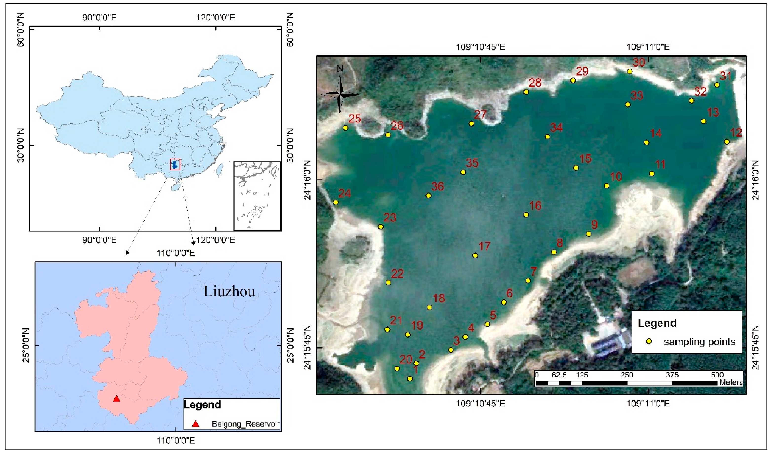
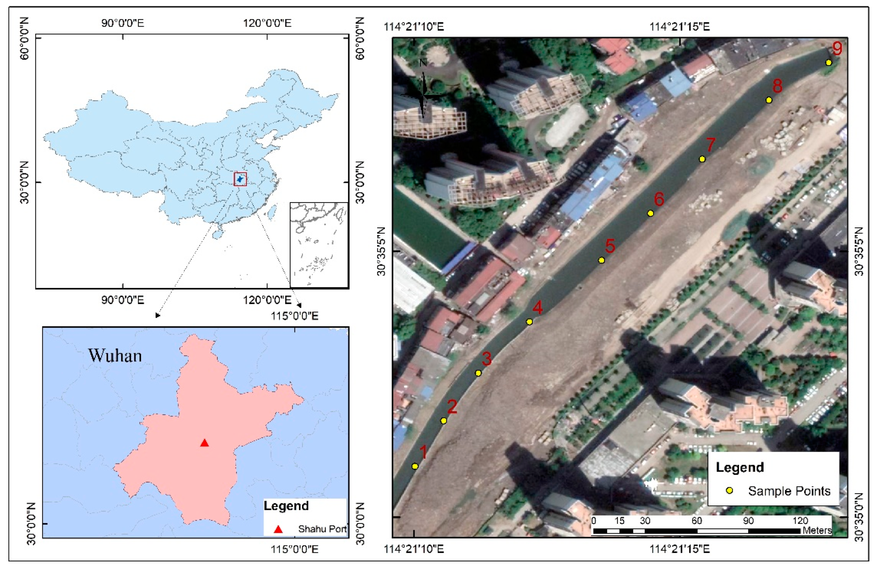
2.1. Study Area

Beigong Reservoir is 16 km away from the county town of Labao in Liuzhou and covers more than 270 Mu. The coordinates are 109°10′E and 24°15′N. The reservoir is surrounded by mountains. Due to its beautiful scenery, the reservoir is known as “Southern Tianchi” and was selected as the most beautiful scenery shooting spot in nine western provinces. As a Case-2 water, it is said to be one of the local drinking water sources and has extremely important research significance.

Shahu Port is located between Shahu in Wuchang District and Donghu Port in Qingshan District. It is a well-known “stinky water port” in Wuhan. The coordinates are 114°21′14.15″E and 30°35′5.52″N. The riverway is under treatment and the pollution level is lower than before. Still, the odor could be smelled, and the water was still muddy by visual observation. We intercepted a section of riverway from Xudong Street to Tieji Road in SP, and evenly laid out nine sampling points.

2.2. Data Collection

On 9–10 September 2018, 36 sampling points were selected, evenly distributed in BR, as shown in Figure 1. Based on the objective external conditions of the field data collection, only 23 of the 36 sampling points were selected for spectral acquisition. On 15 and 16 July 2018, nine sampling points were laid out in SP and the UAV-borne HRS data were collected. Nine ground control points were used for hyperspectral UAV-borne image correction. The distribution of sample points is shown in Figure 2. In addition, 20 water samples and ground spectra were collected in East Lake and Yangtze River in Hankou Beach.

The experimental data acquisition process consisted of three parts: spectral measurement of the water surface, collection and assay of the water samples, and simultaneous acquisition of aerial remote sensing images. The measurement of the water surface spectrum was based on the “above-water method” [16]. This approach was used as the main method for the field measurements by Watanabe et al. [17] and Chen et al. [18]. The acquisition device was an American ASD FieldSpec 3 field portable spectrometer (wavelength range of 350–2500 nm) manufactured by ASD Lnc. (Boulder, Colorado, U.S.A) and provided by China University of Geosciences (Wuhan, China). In addition, auxiliary information, such as latitude/longitude and surface temperature, were also recorded.

The eight-rotor DJ M600 Pro UAV was selected as the airborne platform, and the sensor mounted on it was a Headwall NANO-Hyperspec manufactured by Headwall Photonics Lnc. (Fitchburg, Massachusetts, USA) and provided by Xingbo Keyi Co., Ltd (Guangzhou, China) ultra-micro airborne hyperspectral imaging spectrometer. This unit includes a complete data acquisition storage module and a global positioning system/inertial measurement unit (GPS/IMU) navigation system. The integrated data acquisition system has Gig-E connection, which allows the data to be downloaded during flight. The synchronously acquired global positioning system/inertial navigation system (GPS/INS) data facilitate the subsequent geometric correction. Furthermore, the weight of the spectrometer is only 0.5 kg, which significantly reduces the burden on the UAV. The technical parameters are shown in

Table 1. Headwall NANO-Hyperspec technical parameters.

Class	Parameter			Class	Parameter
Wavelength range	400–1000 nm			Field of view	33	22	16
Number of spectral channels	270			IFOV single pixel spatial resolution	0.9	0.61	0.43
Number of spatial channels	640			Instrument power consumption	<13 W
Spectral sampling interval	2.2 nm/pixel			Bit depth	12 bit
Spectral resolution	6 nm @ 20 µm			Storage	480 GB
Secondary sequence filter	Yes			Cell size	7.4 µm
Numerical aperture	F/2.5			Camera type	COMS
Light path design	Coaxial reflection imaging spectrometer			Maximum frame rate	300 fps
Slit width	20 µm			Weight	<0.6 kg (no lens)
Lens focal length	8 mm	12 mm	17 mm	Operating temperature	0–50 °C

. At BR, the wavelength range is 400–1000 nm and the spatial resolution is 0.173 m. The numbers of spectral channels and spatial channels are 270 and 640, respectively. During the actual flight of the UAV at BR, the flight height relative to the ground was 400 m, and the heading overlap was 80%. Wind speed of 5.2 m/s meets the flight requirements of the UAV. Since the reservoir is surrounded by mountains, considering the flight safety and image width, 10 flight strips were designed to cover the entire lake. During the actual flight of the UAV at SP, the flight height relative to the ground was 100 m, the spatial resolution is 0.044 m, and four flight strips were designed to cover the riverway. Wind speed of 4 m/s meets the flight requirements of UAV. At two study areas, a 17 mm lens with a field of view angle of 16° was selected.

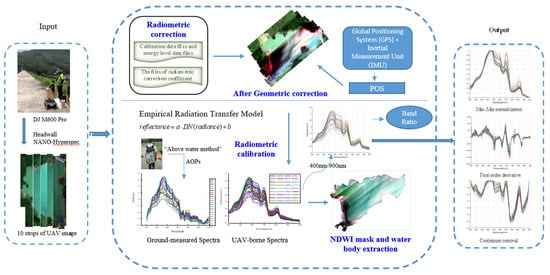
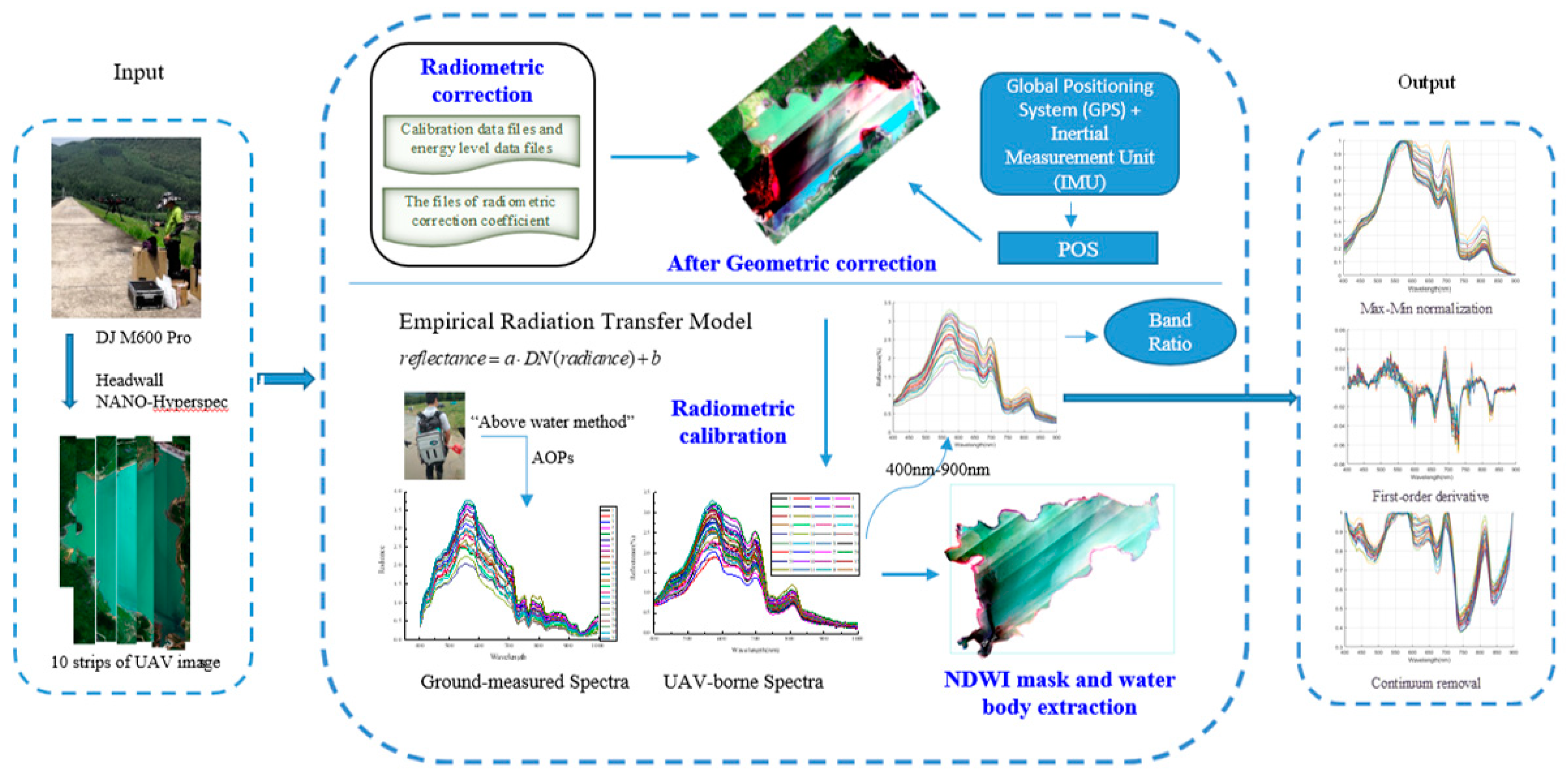
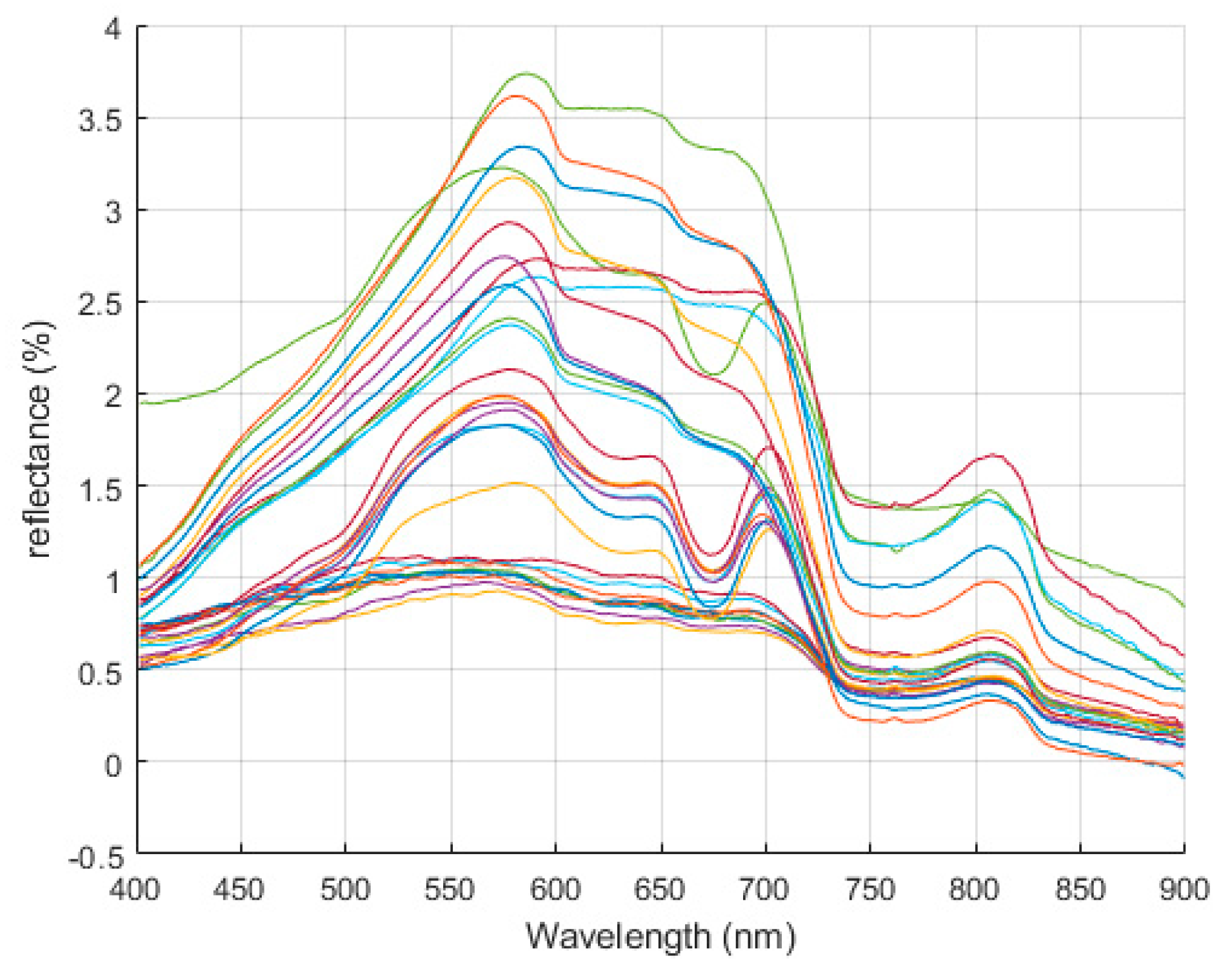
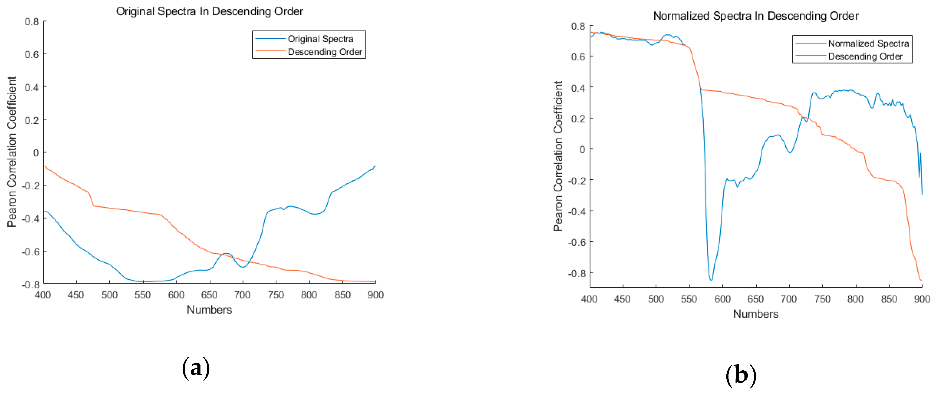
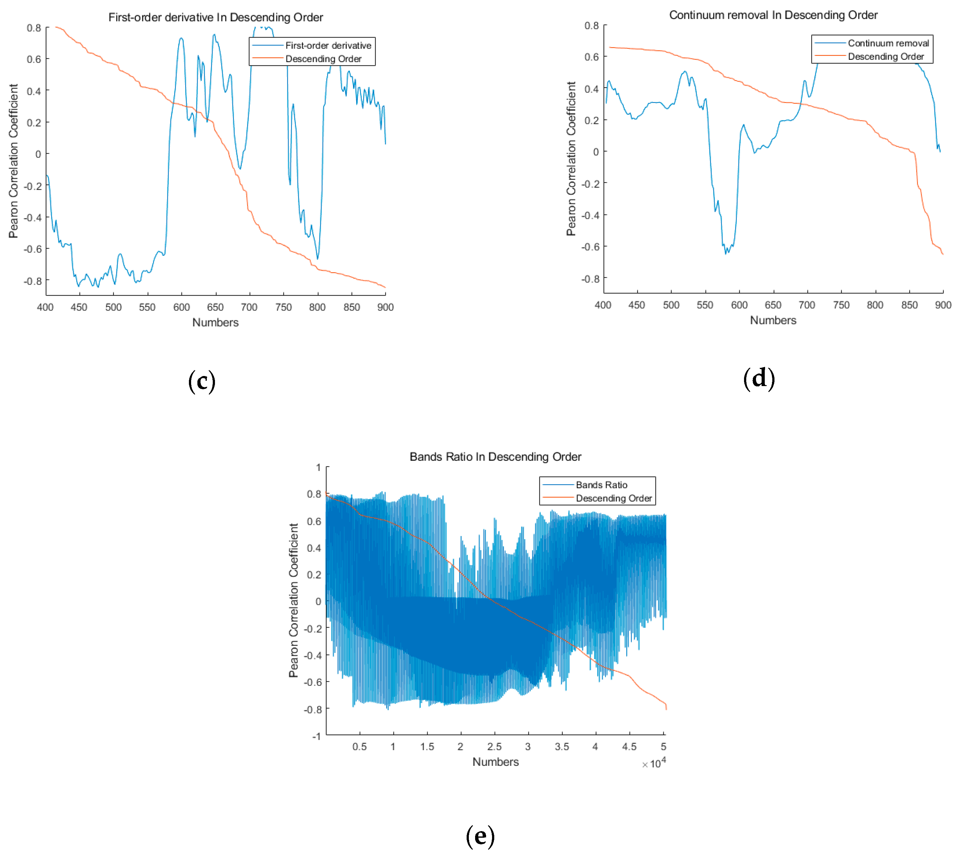
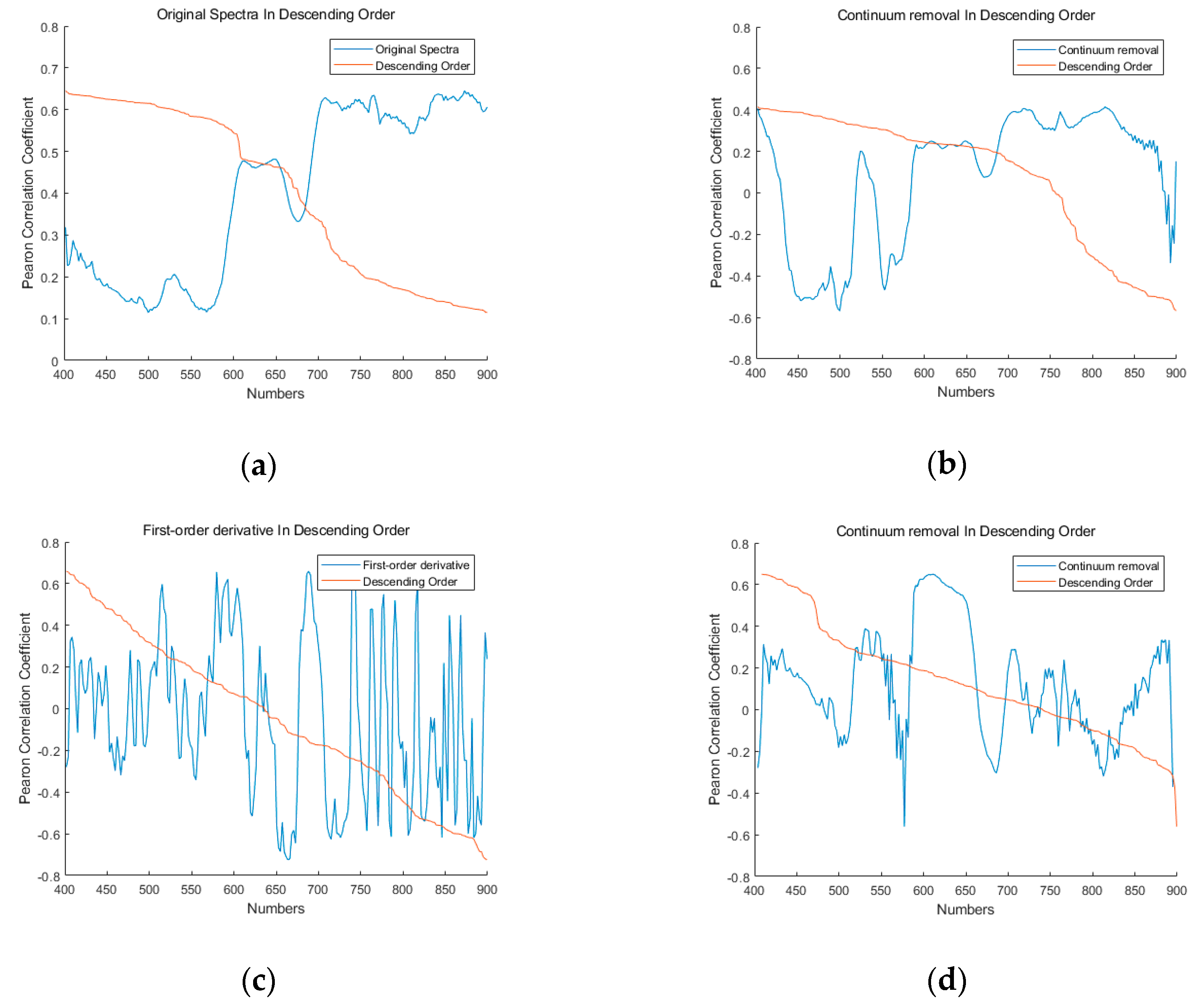
2.3. Preprocessing of the UAV Images and Spectra

In view of the hardware conditions and the experimental requirements, the UAV-borne HRS images were preprocessed as follows: radiometric correction, geometric correction, filtering, masking and water extraction, and spectral extraction of the sample points, as shown in Figure 3. Among these processes, radiometric correction and geometric correction are common processes in remote sensing image processing. Due to the low flying altitude of the UAV, the complex atmospheric effects can be ignored in the radiation calibration in flight. The method is described as follows:

1. The first step was laboratory calibration of the sensor, which involved converting the output signal of each sensor unit to an accurate radiance value.

2. The NANO-Hyperspec hyperspectral imaging spectrometer integrates the sensors and the position and orientation system (POS) by combining differential GPS technology with IMU technology. For geometric correction, the POS data and HRS image data were first matched, and then the coordinate system was transformed to establish the correspondence between the image pixels and the coordinates of the ground control points around the reservoir. Finally, re-sampling was used to establish the corrected images.

3. The next step was radiometric calibration. By obtaining the water-leaving reflectance of the ground sampling points and the pixel spectra of the HRS images after geometric correction, the linear relationship (Equation (1)) between the UAV-borne spectral radiance and the ground-based spectral reflectance was constructed to realize radiometric calibration of the UAV-borne images:

$$reflectance=a\cdot DN(radiance)+b$$

(1)

Since only 23 ground spectra were collected at BR, 23 corresponding spectra on UAV-borne images were obtained for linear fitting. At SP, all ground spectra were applied for radiometric calibration. The calibration program was written by IDL/ENVI, and the linear function fitted by ground spectrum and UAV spectra were applied to the radiation calibration of the whole UAV-borne images.

4. The outputs include the max-min normalization, the first-order differential, the continuum removal, and the band ratio of the original spectra. Later, these datasets will be analyzed through experiments, and appropriate data sets will be extracted for SSC inversion.

The formula for the water-leaving reflectance is as follows [16]:

$$L_w=L_{sw}-r{L}_{sky}$$

(2)

$$E_d(0^{+})=L_p\frac{\pi }{{\rho }_p}$$

(3)

$$R_{rs}=\frac{L_w}{E_d(0^{+})}=\frac{(L_{sw}-r{L}_{sky})}{\pi L_p}{\rho }_p$$

(4)

where $L_w$ is the water-leaving radiance, $L_{sw}$ is the total radiance received by the spectrometer, and $L_{\mathrm{sky}}$ is the sky radiance value. Here, the influence of atmospheric scattering and direct reflection of sunlight is ignored by the certain observation geometry. $E_d(0^{+})$ is the total incident irradiance on the water surface. ${\rho }_p$ is the standard reference plate reflectivity. A reference plate with a reflectivity of nearly 1 was selected in this study. $L_p$ is a signal that is converted to a 100% reference plate. $R_{rs}$ is the water-leaving reflectance.

Spectral normalization reduces the effects of weather conditions and measurement angles on reflectivity, making it convenient to compare measured results from different locations and different times [19,20]. The first-order differential model can remove the influence of semi-linear or near-linear background and noise on the target spectrum [21]. The continuum removal method is a relatively common method in mineral analysis, which makes it possible to compare the absorption characteristics of the reflectance spectrum on a common baseline [22]. The band ratio model not only partially compensates for atmospheric effects, but it also eliminates the interference of water surface roughness and ambient noise [23]. Therefore, based on the influence of the above spectral pretreatment methods on the content of the subsequent SSC inversion, after extracting the spectra of the 32 reflectance curves in the UAV imagery with the wavelength range of 400–900 nm, the pretreatment included normalization, first-order differential pretreatment, and continuum removal. The different pretreatment methods were compared to evaluate their impact on the experimental data.

2.4. Methods

2.4.1. Support Vector Machine and Least Squares Support Vector Machine

Cortes and Vapnik [24] first proposed the concept of SVM in 1995. SVM is based on the Vapnik-Chervonenkis dimension theory of statistical learning and the principle of structural risk minimization. When solving the problems of small sample size, nonlinear, and high-dimensional pattern recognition, it has its own unique advantages. The SVM kernel is now embedded in many machine learning toolkits, including LIBSVM, MATLAB, SAS, SVMlight, Scikit-Learn, OpenCV, etc., so it is easy to carry out the related algorithms and theoretical research.

Mapping samples from the original space to a higher-dimensional feature space by the kernel, therefore, if the choice of kernel is not suitable, this means that mapping the sample from the original space to an unsuitable feature space will directly lead to poor performance of the algorithm.

At present, the commonly used kernels are as follows:

1. Linear kernel:

$$K(x_i,x_j)=x_i{}^T\cdot x_j$$

(5)

The linear kernel function is the simplest kernel function, and it represents the dot product of any two sample points in the space after the expansion.

2. Polynomial kernel:

$$K(x_i,x_j)={(x_i{}^T\cdot x_j)}^d$$

(6)

where $d\ge 1$ is the degree of the polynomial. When $d=1$, it degenerates into a linear kernel.

3. Radial basis function (RBF) kernel:

$$K(x_i,x_j)=\exp (-\frac{{\Vert x_i-x_j\Vert }^2}{2{\sigma }^2})$$

(7)

where $\sigma >0$ is the bandwidth of the Gaussian kernel.

Suppose there is a sample $\left(x_1,y_1\right),\left(x_2,y_2\right),\dots ,\left(x_n,y_n\right)\in R^n\times R$. Firstly, the sample is mapped from a low-dimensional space Rⁿ to a high-dimensional space $\Psi \left(x\right)=(\phi (x_1),\phi (x_2),\dots \phi (x_3))$ through a nonlinear mapping $\Psi \left(x\right)$. In this high-dimensional feature space, the best decision function is constructed as follows:

$$y(x)=w\cdot \phi (x)+b$$

(8)

Support vector machine regression can be seen as the use of a hyperplane to fit the sample data, using the principle of structural risk minimization, to find the appropriate w and b under the constraints of inequality, so that the decision function is minimized:

$$\min :J(w,\xi )=\frac{1}{2}{\Vert w\Vert }^2+c{\displaystyle \sum _{i=1}^N{\xi }_i{}^2}$$

(9)

$$y_i[w\cdot \phi (x_i)+b]\ge 1-{\xi }_i,i=1,\dots ,N$$

(10)

$${\xi }_i\ge 0,i=1,\dots ,N$$

(11)

The first term in Equation (9) is the objective function, which controls the complexity of the model. The second term is the function of the control error, where ${\xi }_i$ is the slack variable and c is the penalty coefficient that minimizes the error.

In 1999, Suykens [25] proposed a new SVM model known as the least-squares support vector machine (LSSVM) model. LSSVM uses a least-squares linear system as the loss function, instead of the quadratic regression method used in the traditional SVM. This conversion greatly simplifies the problem, making the solution process have linearly provided features or, rather, the Karush–Kuhn–Tucker (KKT) linear system [26]. The optimization goal of LSSVM becomes an equality constraint from the inequality constraint problem, so the optimization problem becomes different from that of the SVM:

$$\min :J(w,\xi )=\frac{1}{2}{\Vert w\Vert }^2+\frac{\gamma }{2}{\displaystyle \sum _{i=1}^N{\xi }_i{}^2}$$

(12)

$$s\cdot t:y_i=\phi (x_i)\cdot w+b+{\xi }_i,i=1,\dots ,N$$

(13)

where $\gamma$ is the regularization parameter and ${\xi }_i$ is the slack variable. The Lagrange optimization method and KKT are used to solve Equations (12) and (13) to obtain the nonlinear equation:

$$f(x)={\displaystyle \sum _{i=1}^N{a}_{i}K(x_i,y_i)+b}$$

(14)

where $a$ and $b$ are the solutions of the linear equations in the process of solving Equation (14). $K(x_i,y_i)$ is the selected kernel function.

Since the least-squares method is used in the process of the solution, the new SVM model is called LSSVM. Compared to the standard SVM, LSSVM uses the least-squares method, which is faster and consumes less resources [27]. However, the LSSVM regression process is similar to that of SVM. It is especially important to choose the appropriate regularization parameter $\gamma$ and kernel function parameter. The larger the value of $\gamma$, the larger the loss function will be. This means that the model is reluctant to give up further outliers, which would generate more support vectors and directly lead to the hyperplane becoming too complicated and over-fitted. In contrast, if $\gamma$ is too small, the under-fitting phenomenon can easily occur. Therefore, if $\gamma$ is too large or too small, the fitting accuracy is lowered. In this paper, RBF is chosen as the kernel function, and the Gaussian kernel bandwidth $\sigma$ has a great influence on the model. Parameter $\sigma$ represents the effect of a single sample on the entire hyperplane. When $\sigma$ is too small, a single sample has a large influence on the hyperplane, and then more samples are selected as support vectors. When $\sigma$ is too large, the model will be too constrained to fit the complex shape of the data. Therefore, in this paper, PSO is selected to optimize the regularization parameter $\gamma$ and Gaussian kernel bandwidth $\sigma$ of the LSSVM model, to reduce the inaccuracy and excessive time required when manually selecting the best parameters.

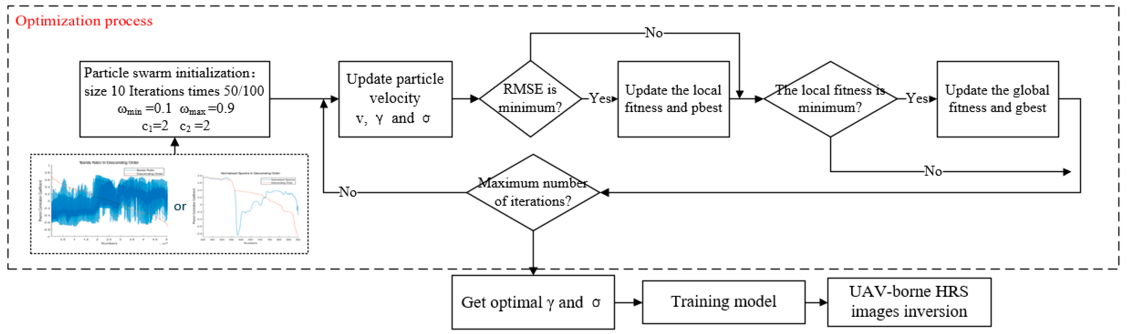
2.4.2. Particle Swarm Optimization Algorithm

Particle swarm optimization (PSO) is a new evolutionary algorithm (EA) developed by Kennedy and Eberhart [28] in 1995. After, researchers repeated experiments to eliminate irrelevant parameters and obtained the initial PSO model [29]. Then, in 1998, the concept of adding inertia weights to the PSO algorithm was first published [30], where the formulas of the velocity and position of the particle are obtained as follows:

$$V_{id}=\omega V_{id}+C_{1}random(0,1)(pbes{t}_{id}-X_{id})+C_{2}random(0,1)(gbes{t}_{id}-X_{id})$$

(15)

$$X_{id}=X_{id}+V_{id}$$

(16)

Equation (15) represents the d-dimensional velocity update formula of particle i. The first item indicates the previous speed of the particle. The second part shows the distance between the current position of particle i and its best position. The third part shows the distance between the current position of particle i and the best position of the group. Equation (16) represents the d-dimensional position update formula of particle i. $V_{id}$ indicates the speed of the particle. $random(0,1)$ is a random number between [0, 1]. $pbes{t}_{id}$ represents the local optimal position of the i-th particle in the d-th dimension. $gbes{t}_{id}$ represents the global optimal position in the d-th dimension.

Before the particle swarm algorithm is executed, the initial particle swarm state needs to be set in advance. The group size is usually 20–40, but for complex problems it can be 100–200. The maximum number of iterations (stopping criterion) specifies when the inertia factor stops in the iterative optimization. Acceleration constants $c_1$ and $c_2$ adjust the maximum step size of the learning, and generally $c_1=c_2\in (0,4]$. The inertia factor $\omega$ is non-negative. When the model is large, the global optimization ability of the model is strong, and the approximate position of the optimal solution can be determined quickly, but the local optimization ability of the model is weak. As $\omega$ decreases, the particle velocity slows down, resulting in a strong local optimization ability for the model, which can be finely localized in the local region, thus accelerating the convergence speed [31].

Since the concept of the PSO algorithm was first proposed, as the scope of the application continues to expand, PSO algorithms have been developed with different development directions in different application fields. Kumar and Janga Reddy added a new strategy mechanism (elitist mutation) to improve the performance of the standard PSO algorithm, which was applied to the Bhadra Reservoir system providing irrigation and hydropower in India [32]. Sedki and Ouazar combined PSO and differential evolution (DE) methods for the design of water distribution systems, to reduce costs [33]. Based on the above theory and application practices, LSSVM has been confirmed to have the ability to solve problems of small sample size and nonlinear regression, and it has the advantages of a strong generalization ability, fast convergence, and low resource consumption. Considering the advantages of particle swarm optimization, including the simple and easy operation, fast convergence, and less setting of parameters in the parameter optimization, we decided to use the PSO algorithm for the optimization of the regularization parameters and the Gaussian kernel bandwidth of the LSSVM model, to solve the problem of the inversion accuracy of SSC not being high for BR.

2.4.3. Statistical Analysis

In this study, a variety of models were used to invert the WQPs. Since the modeling process was implemented in two editing environments, MATLAB and Python, and the library functions used were different, there will be some differences in the accuracy evaluation. Therefore, the accuracy of the inversion results was unified by the coefficient of determination ($R^2$), the root mean square error (RMSE) [34], and the mean absolute percentage error (MAPE).

The coefficient of determination ($R^2$):

$$\overline{y}=\frac{1}{n}{\displaystyle \sum _{i=1}^n{y}_i}$$

(17)

$$S{S}_{tot}={{\displaystyle \sum _i(y_i-\overline{y})}}^2$$

(18)

$$S{S}_{reg}={{\displaystyle \sum _i(f_i-\overline{y})}}^2$$

(19)

$$S{S}_{res}={{\displaystyle \sum _i(y_i-f_i)}}^2={\displaystyle \sum _i{e}_i^2}$$

(20)

$$R^2=1-\frac{S{S}_{res}}{S{S}_{tot}}=\frac{S{S}_{reg}}{S{S}_{tot}}$$

(21)

where $S{S}_{tot}$ is the sum of squares for the total (SST), $S{S}_{reg}$ is the sum of squares for the regression (SSR), and $S{S}_{res}$ is the sum of squares for the error (SSE). $R^2$ ranges from [0, 1]. The greater the model’s goodness of fit, the higher the degree of interpretation of the dependent variable by the independent variable, the denser the observation points are near the regression line, and the closer the $R^2$ value is to 1.

RMSE, MAPE: in the case of one predictor variable, RMSE and MAPE are defined as:

$$RMSE=\sqrt{\frac{1}{N}{\displaystyle \sum _{i=1}^N{(X_{Obs,i}-X_{Est,i})}^2}}$$

(22)

$$MAPE=\frac{1}{N}{\displaystyle \sum _i^N\frac{\left|X_{Est,i}-X_{Obs,i}\right|}{X_{Obs,i}}}\times 100\%$$

(23)

where N is the total number of observations in the dataset, $X_{Obs,i}$ is the observed in situ value, and $X_{Est,i}$, i is the estimated value.

RMSE is sensitive to outliers, but it can truly reflect the deviation between the quantitative inversion results of suspended solids concentration and the discrete sampling results in the field, which enables the analysis of accuracy improvement available through the use of UAV-borne spectral data. In order to further consider the ratio between the error and the true value, the quantitative performance index MAPE was used. $R^2$ can reflect the fitting degree of spectrum to water quality parameters well. The higher $R^2$ is, the more intensive the prediction results and ground samples are near the regression line, and the more intuitive the fitting degree is.

Correlation is a very important part of the modeling process, so in order to avoid any difference in correlation coefficients due to the different modeling environments, Pearson’s correlation coefficients were uniformly used.

3. Experiments and Analysis

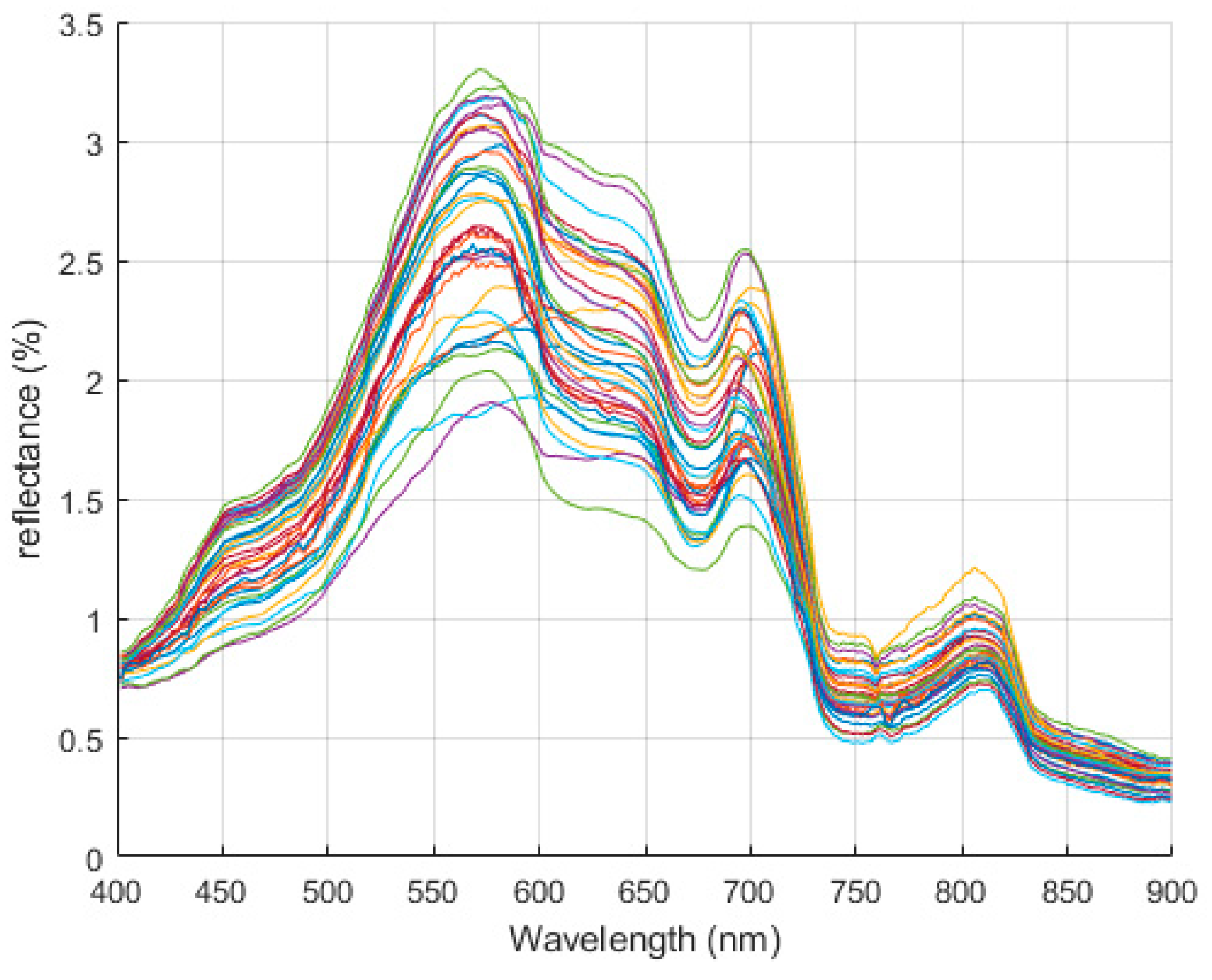
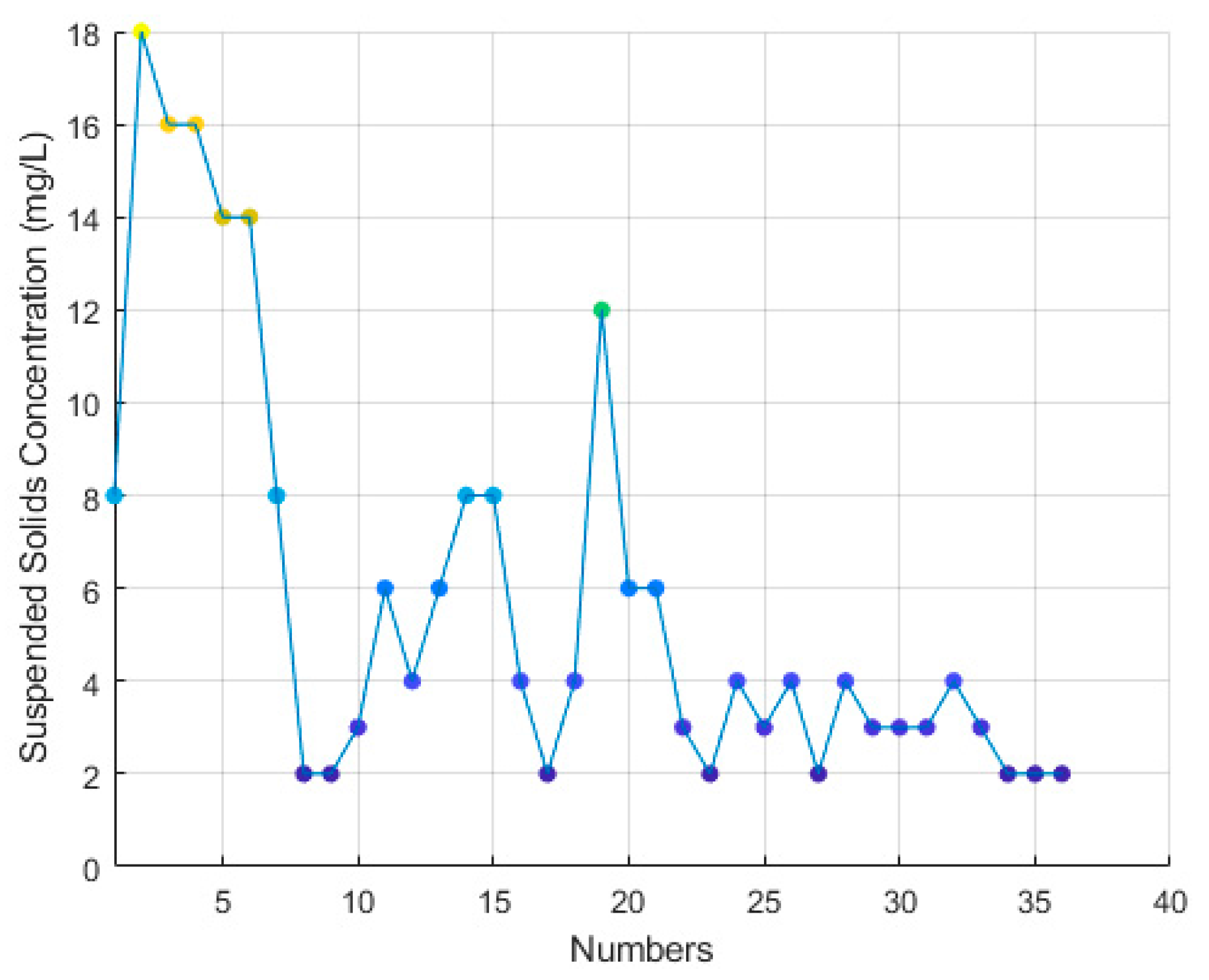
3.1. Data Analysis of Beigong Reservoir Samples

According to the GPS locations of the 36 sample points, after the preprocessing of the UAV-borne HRS images, the spectral curves of the remote sensing reflectance obtained from the images are shown in Figure 4. Distinct bimodal characteristics are apparent in the reflectance curves. The main reflection peak appears in the wavelength range of 560–590 nm, and the secondary reflection peak is located in the infrared band between 790 nm and 900 nm. Since the overall SSC in the reservoir is low, the first peak is formed above the second peak. A reflection peak appears at a wavelength of 700 nm. When the SSC increases, the reflection peak moves toward the long wave direction (“red shift”) [35]. Therefore, the curves of the remote sensing reflectance have the obvious spectral characteristics of suspended solids and can be used for the study of SSC inversion.

The 36 water samples were tested in the laboratory, and a line chart of the SSC is shown in Figure 5. The SSC values of samples 1–6 and 19 were high, generally exceeding 10 mg/L. Sample 2 had the highest concentration of 18 mg/L. Conversely, the test results of samples 22–36 were at a lower level. When combined with Figure 1, it is further found that the turbid area is generally concentrated in the west bank of the reservoir, especially in the southwest direction near the shore, while the SSC at the north bank is at a medium level.

Table 2. Descriptive statistics for the SSC of the water samples from BR dataset.

n	Max $(\mathbf{m}\mathbf{g}\cdot {\mathbf{L}}^{-1})$	Min $(\mathbf{m}\mathbf{g}\cdot {\mathbf{L}}^{-1})$	Mean $(\mathbf{m}\mathbf{g}\cdot {\mathbf{L}}^{-1})$	SD $(\mathbf{m}\mathbf{g}\cdot {\mathbf{L}}^{-1})$	CV
36	18.00	2.00	5.86	4.61	0.79

lists the descriptive statistical information of the SSC, including the number of samples, the minimum (Min), the Maximum (Max), the mean, the standard deviation (SD) and the coefficient of variation (CV). The SSC is low overall (Min = 2 mg/L, Max = 18 mg/L, mean = 5.86 mg/L, SD = 4.61 mg/L, CV = 0.79), which is in line with the actual water quality conditions of a drinking water source. The standard deviation is 4.61 mg/L, which is slightly less than the mean value, and the degree of data variation is not large. Therefore, it can be preliminarily judged that there are no abnormal sample points, and that the test results of the 36 samples can be used for the SSC estimation.

After the spectral curves of the remote sensing reflectance extracted from the UAV-borne HRS images were preprocessed by maximum and minimum normalization, first-order differential pretreatment, continuum removal, and the band ratio model, Pearson’s correlation analysis was performed between the spectral curves and the WQPs (such as SSC). The results of the correlation coefficients in descending order are shown in Figure 6. The maximum positive correlation coefficient between the original remote sensing reflectance and SSC is 0.65 (Figure 6a). There are 58 spectral correlation coefficients higher than 0.6, which are mainly concentrated in the 700–900 nm band, indicating that the reflectivity of this band range is sensitive to changes in SSC. Gitelson [12] stated that the 700–900 nm band is the best band for remote sensing inversion of SSC. Compared with the original spectra, the correlation coefficient of the max-min normalization (Figure 6b) decreases in the maximum positive correlation, the largest negative correlation increases to −0.57, and the overall correlation increases insignificantly. The correlation coefficient of the first-order differential pretreatment (Figure 6c) shows no significant change in the maximum positive correlation, but the largest negative correlation of −0.73 appears near the 660 nm band. The continuum removal (Figure 6d) result shows high correlation in the 600–650 nm band, but the overall improvement is not obvious compared to the original remote sensing reflectance.

The band ratio model can eliminate the interference of water surface roughness and background noise, and is thus a commonly used contrast enhancement operation in remote sensing quantitative inversion. The exhaustive method was used to calculate the band ratio. By calculating the ratio of the 225 bands with each other, 50,400 characteristic variables were obtained. The Pearson’s correlation coefficients of each characteristic variable with SSC were then calculated, and are arranged in descending order in Figure 6e. The results show that the maximum correlation coefficient is 0.73, the correlation coefficient of 135 characteristic variables is greater than 0.7, and the maximum negative correlation is −0.72. Compared with the other spectral pretreatments, the correlation of the band ratio model result is increased significantly. Therefore, the band ratio model is suitable for the study of SSC inversion modeling.

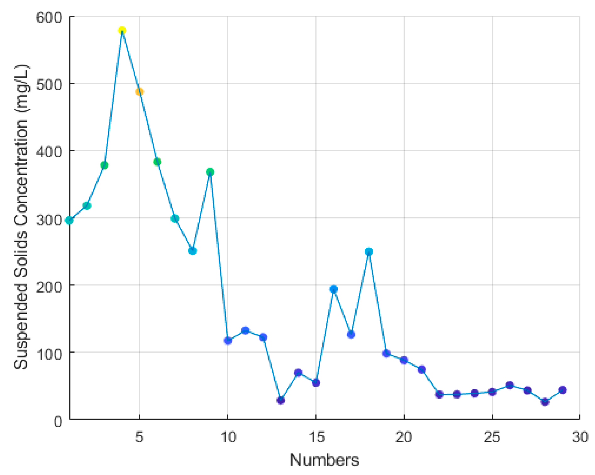
3.2. Data Analysis of Shahu Port Samples

The spectral waveform (Figure 7) collected in the study area is similar to that in the first study area, but the spectral reflectance (near 1%) of the polluted riverway is lower than East Lake and the Yangtze River. This is due to the comprehensive effect of various WQPs such as water-insoluble particulate matter, colored dissolved organic matter (CDOM), and chlorophyll-a (Chl-a) [36,37]. The absorption coefficient of CDOM in polluted water is high, while the backscattering of water is controlled by inorganic particulate matter. The common contribution of various factors results in “low scattering and high absorption” of the riverway. The quantitative inversion method based on statistical methods explores the relationship between a single water quality index and the spectra above the water surface without considering the complex underwater optical field. This is significant for the discussion of quantitative inversion technology based on UAV hyperspectral data.

A total of 29 bottles of water samples were collected from SP, East Lake, and the Yangtze River. The concentration curve of suspended solids in laboratory tests is shown in Figure 8. Sample points 1–9 came from SP, and the SSC was above 200 mg/L, while SSC in East Lake and the Yangtze River was relatively low. According to the descriptive statistics (

Table 3. Descriptive statistics for the SSC of the water samples from the SP dataset.

n	Max $(\mathbf{m}\mathbf{g}\cdot {\mathbf{L}}^{-1})$	Min $(\mathbf{m}\mathbf{g}\cdot {\mathbf{L}}^{-1})$	Mean $(\mathbf{m}\mathbf{g}\cdot {\mathbf{L}}^{-1})$	SD $(\mathbf{m}\mathbf{g}\cdot {\mathbf{L}}^{-1})$	CV
36	578.00	26.64	173.74	154.64	0.89

), the overall SSC in the second study area (Min = 26.64 mg/L, Max = 578 mg/L, mean = 173.74 mg/L, SD = 154.64 mg/L, CV = 0.89) is higher than in BR, which involves different water quality conditions in different waters.

The Pearson correlation coefficients between the spectra of the second study area images after preprocessing and suspended matter concentration are shown in Figure 9. There was no positive correlation between original remote sensing reflectance (Figure 9a) and SSC, and the maximum negative correlation of −0.789 appears near the 557 nm band. After normalization (Figure 9b), the correlation between spectra and SSC increased significantly. The correlation between 400–552 nm is greater than 0.6, and the maximum negative correlation of −0.85 appears near the 581 nm band. Compared with the correlation of the original spectra with the WQPs (such as SSC), the first order differential (Figure 9c), the continuum removal (Figure 9d) and the band ratio (Figure 9e) have improved, but they have little change compared with the normalization. In addition, considering the influence of spectral normalization on eliminating the differences caused by different observation environments and the difficulty of UAV image processing, the normalized spectra were selected as the input variables of LSSVM.

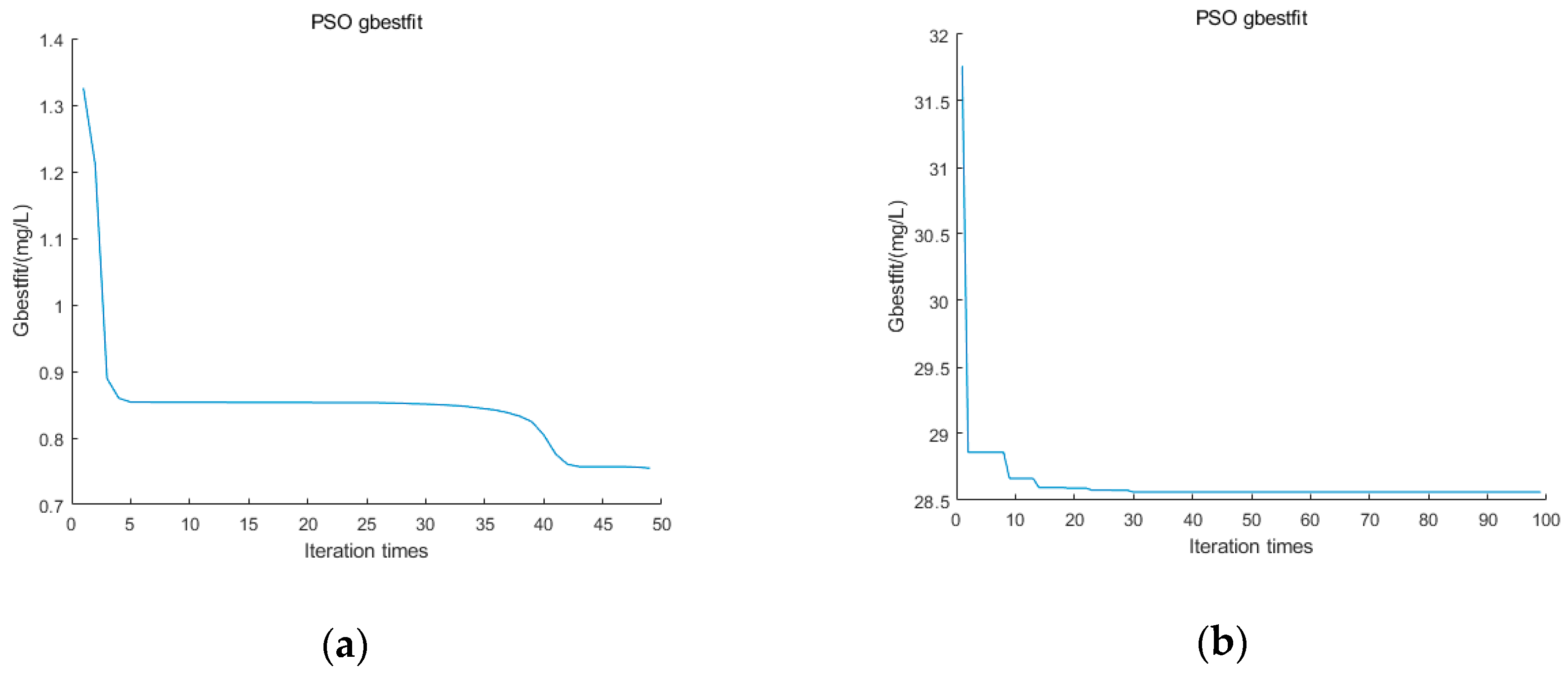
3.3. Particle Swarm Optimization-based Least Squares Support Vector Machine Modeling

The training samples were uniformly selected in the study area, and the PSO-LSSVM algorithm was used to model the SSC inversion, as shown in Figure 10. For BR dataset, the ratio models whose correlation coefficient with SSC was greater than 0.7 were selected as the input variable of the PSO-LSSVM model, and the predicted SSC was used as the output variable.

Firstly, the initial state of the particle swarm needed to be set before undertaking the PSO optimization. The default values were used except for the particle size (5, 10, 15, 20…) and the maximum iteration (50, 100, 150, 200, …). We attempted different particle sizes and maximum iterations by enumeration to prevent the LSSVM model from over-fitting. Finally, for the BP dataset, we confirmed the particle size = 10, maximum iteration = 50, extreme value of inertia factor (${\omega }_{\min }$ = 0.1, ${\omega }_{\max }$ = 0.9), and acceleration constant ($c_1$ = 2, $c_2$ = 2). The initial values of the particle velocity and position were calculated based on the initial state of the particle swarm. For the SP dataset, the maximum iteration = 100, and the other parameters were the same.

During the iteration, the RMSE of the predicted result was calculated each time, as well as the current local and global fitness of the particle, i.e., pbest and gbest. At the same time, the inertia factor $\omega$ was calculated according to the formula $\omega ={\omega }_{\max }-(ite{r}_i-1)\cdot ({\omega }_{\max }-{\omega }_{\min })/iter$, where iter represents the number of iterations.

When entering the next iteration, pbest and gbest were used to update the current particle velocity and position. This method was iterated sequentially until the maximum number of iterations was reached. If the stopping condition was not met, the speed and position of the particle were continued to be updated. After stopping the iteration, the LSSVM model was trained according to the currently obtained optimal parameters. Due to PSO, one of optimization methods, it is not necessary to directly tune LSSVM parameters. After iteration, PSO calculated a and b (Equation (13)) at the minimum fitness. Finally, the UAV-borne HRS image inversion was performed using this model.

Figure 11 shows the fitness curve of the PSO optimization process. For BR, it can be seen that the PSO quickly converges at the beginning of the optimization process, where the fitness value decreases significantly, and then remains at 0.85 mg/L. When iterating nearly 40 times, the fitness decreases slightly to 0.75 mg/L and then remains stable again. At this time, $R^2$ (0.98), RMSE (0.68 mg/L), and MAPE (12.66%) values remain at a good level. When the data of the second study area were used as input variables, the root mean square error decreased from 32.18 mg/L to 28.56 mg/L, and it did not change after 20 iterations.

To verify the validity of the model, the remaining samples were used as test samples to estimate the SSC. The inversion results of the training set and test dataset are shown in Figure 12. The predicted values and the true values of all the samples are evenly distributed on the diagonal, indicating that the inversion results are good, and that the model can be used for the inversion of SSC.

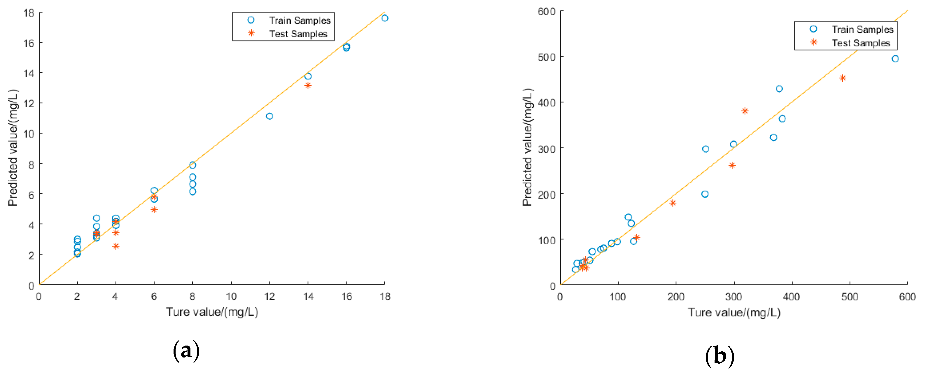
3.4. Accuracy Evaluation of the PSO-LSSVM and Other Models

The SSC inversion of inland waters is still a popular and difficult problem. Scholars have proposed a large number of classical algorithm models for the modeling and prediction of WQPs. Doxaran et al. [38] proposed the use of the sensitivity of the near-infrared band to SSC for the Gironde estuary in France, and modeled the SSC using the band ratio model. Therefore, in this study, we attempted to use the band ratio model to predict the SSC in a variety of common remote sensing inversion models, including exponential function (EF), logarithmic function (LogF), quadratic polynomial (QP), linear function (LinF), and power function (PF) models, to explore whether the traditional empirical or semi-empirical methods were suitable for the inversion of the WQPs of inland waters. For BR, the correlation coefficient between the ratio of the remote sensing reflectance ($R_{595}/R_{499}$) and SSC reached a maximum of 0.733. The ratio ($R_{595}/R_{499}$) was used as the input variable of the above five empirical models, and SSC was used as the output variable. The inversion accuracy results are listed in

Table 4. Comparison of the different methods used to build the models for BR dataset.

Modeling Method	Independent Variables	Mathematical Model	Training Data			Test Data
			R2	RMSE $(\mathbf{m}\mathbf{g}\cdot {\mathbf{L}}^{-1})$	MAPE	R2	RMSE $(\mathbf{m}\mathbf{g}\cdot {\mathbf{L}}^{-1})$	MAPE
PSO-LSSVM	135(number)	—	0.980	0.68	12.66%	0.950	0.75	13.38%
Cars-PLS	135(number)	—	0.522	3.33	58.93%	0.580	2.19	47.44%
RF	135(number)	—	0.799	2.16	43.16%	0.888	1.13	17.56%
EF	$R_{595}/R_{499}$	$a\cdot \exp (b\cdot x)$	0.586	3.10	52.38%	0.791	1.55	31.94%
LogF	$R_{595}/R_{499}$	$a\cdot \log (x)+b$	0.508	3.38	61.85%	0.650	2.01	44.68%
QP	$R_{595}/R_{499}$	$a\cdot x^2+b\cdot x+c$	0.596	3.06	53.77%	0.804	1.50	27.50%
LinF	$R_{595}/R_{499}$	$a\cdot x+b$	0.517	3.35	60.66%	0.665	1.96	43.90%
PF	$R_{595}/R_{499}$	$a\cdot x^b$	0.586	3.10	51.51%	0.780	1.59	33.31%

. For second study area SP, after normalization, the band ($R_{581}$) with the highest correlation with SSC was selected as the input variable of five semi-empirical models. The retrieval results are shown in

Table 5. Comparison of the different methods used to build the models for SP dataset.

Modeling Method	Independent Variables	Mathematical Model	Training Data			Test Data
			R2	RMSE $(\mathbf{m}\mathbf{g}\cdot {\mathbf{L}}^{-1})$	MAPE	R2	RMSE $(\mathbf{m}\mathbf{g}\cdot {\mathbf{L}}^{-1})$	MAPE
PSO-LSSVM	225(number)	—	0.957	31.63	17.96%	0.964	28.56	13.12%
Cars-PLS	225 (number)	—	0.557	101.31	87.06%	0.609	94.63	101.2%
RF	225 (number)	—	0.810	66.38	41.87%	0.740	77.21	47.30%
EF	$R_{581}$	$a\cdot \exp (b\cdot x)$	0.640	91.36	98.48%	0.489	108.16	99.30%
LogF	$R_{581}$	$a\cdot \log (x)+b$	0.743	77.22	59.71%	0.661	88.08	45.96%
QP	$R_{581}$	$a\cdot x^2+b\cdot x+c$	0.748	76.48	59.32%	0.709	81.67	38.98%
LinF	$R_{581}$	$a\cdot x+b$	0.743	77.10	59.61%	0.666	87.51	45.14%
PF	$R_{581}$	$a\cdot x^b$	0.655	89.35	81.70%	0.489	108.13	84.57%

.

In addition, the competitive adaptive reweighted sampling (CARS) algorithm combined with partial least squares (PLS) and RF regression models was also in the comparison experiments (Table 4 and Table 5).

Information redundancy is sometimes caused by too many feature variables, and some useless information may be mixed, which, in turn, reduces the inversion accuracy. The CARS algorithm can solve such a problem. CARS selects the wavelengths with large absolute values of regression coefficients in the PLS model through adaptive reweighted sampling (ARS) technology, and removes the wavelengths with low weights, thus playing the role of characteristic band selection. PLS has the advantages of the three analytical methods of principal component analysis, canonical correlation analysis, and multiple linear regression analysis. PLS is, thus, widely used in water quality parameter inversion. The fitting process of PLS does not involve parameter adjustment. However, before fitting, the CARS algorithm should be applied to select effective characteristics. The number of Monte Carlo sampling runs selected was 50.

The RF algorithm is one of the most commonly used algorithms at present, and its training speed and precision are high, making it popular with many researchers. Even if the algorithm is based on no parameter adjustment, as long as enough trees are used, the predicted results of the model will not show too much offset. Therefore, the RF algorithm was also introduced as a comparison to verify its practicability in predicting SSC. For BR dataset, the maximum number of features used by a single decision tree (MNF = 3) and number of subtrees established (NS = 5) is simply adjusted. When MNF and NS continued to increase, over-fitting was unavoidable, and the accuracy of test data no longer increased. For SP dataset, we tried several different values of MNF (1, 2, 3, 4, 5, …, 10) and NS (5, 10, 20, 30, …, 100), and confirmed MNF = 2 and NS = 6. Other parameters are default values and not adjusted.

In Table 4, comparing the inversion results of all the models, PSO-LSSVM shows the best effect in predicting SSC. Although the prediction accuracy of the test dataset ($R^2$ = 0.95, RMSE = 0.75 mg/L, MAPE = 13.38%) is lower than the prediction accuracy of the training set ($R^2$ = 0.98, RMSE = 0.68 mg/L, MAPE = 12.66%), based on the fact that the minimum value of the actual measured SSC is only 2 mg/L, the inversion result is very good. In addition, the RF regression model also shows good performance ($R^2$ = 0.888, RMSE = 1.13 mg/L, MAPE = 17.56%) in estimating the SSC of the training data, and the inversion accuracy is only slightly lower than that of PSO-LSSVM. Therefore, the RF algorithm could also be used as a research direction for water quality parameter inversion, providing more reference for water quality monitoring methods. However, compared with the RF and PSO-LSSVM models, the prediction effect of the other models is far from ideal. The $R^2$ values of the training data are always less than 0.6, and the RMSE is generally above 3 mg/L. The effectiveness of the prediction results cannot be guaranteed at this low concentration of suspended solids. One difference with PSO-LSSVM is that the test data of the other models predict better results than the training data. The prediction accuracy of the verification data of the quadratic polynomial is very good ($R^2$ = 0.804, RMSE = 1.5 mg/L, MAPE = 27.5%), and the prediction ability is second only to the RF algorithm.

In Table 5, similarly, PSO-LSSVM is the best approach to retrieve SSC. The fitting accuracy of validated data ($R^2$ = 0.964, RMSE = 28.56 mg/L, MAPE = 13.12%) is slightly better than that of the training data ($R^2$ = 0.957, RMSE = 31.63 mg/L, MAPE = 17.96%). RF has good performance both in training data fitting ($R^2$ = 0.810, RMSE = 66.38 mg/L, MAPE = 41.87%) and test data retrieval ($R^2$ = 0.740, RMSE = 77.21 mg/L, MAPE = 47.30%). Compared with BR, the five semi-empirical models in SP all perform well, especially LogF, QP, and LinF, whose accuracy of training data are close to 0.75, which is much better than the semi-empirical model in BR. It is speculated that this may be related to the high correlation between the input variables of modeling and the retrieved WQPs.

In summary, regarding the SSC inversion based on UAV-borne HRS images, several inversion models were compared for two study areas. In the areas, the overall performance of multiple models is generally consistent. We found that PSO-LSSVM is better than other classical models. When the input variables are the same, RMSE shows the advantages and disadvantages of the inversion results of different models. The output of LSSVM model is closer to the fitting curve. Then, comparing the inversion results of different study areas by using the determinant coefficients and MAPE, PSO-LSSVM performed well in both areas, which proved that the model was suitable for the current datasets. In addition, we also found that Random forest had a good performance both in the simplicity of super-parameters adjustment and inversion accuracy, and this model can be studied in the future. The fitting results of semi-empirical model are stable. Comparing the two study areas, it is found that higher the correlation between water quality parameters and input variables is, higher the inversion accuracy of semi-empirical models. However, the PLS method with feature extraction is not suitable for the current datasets.

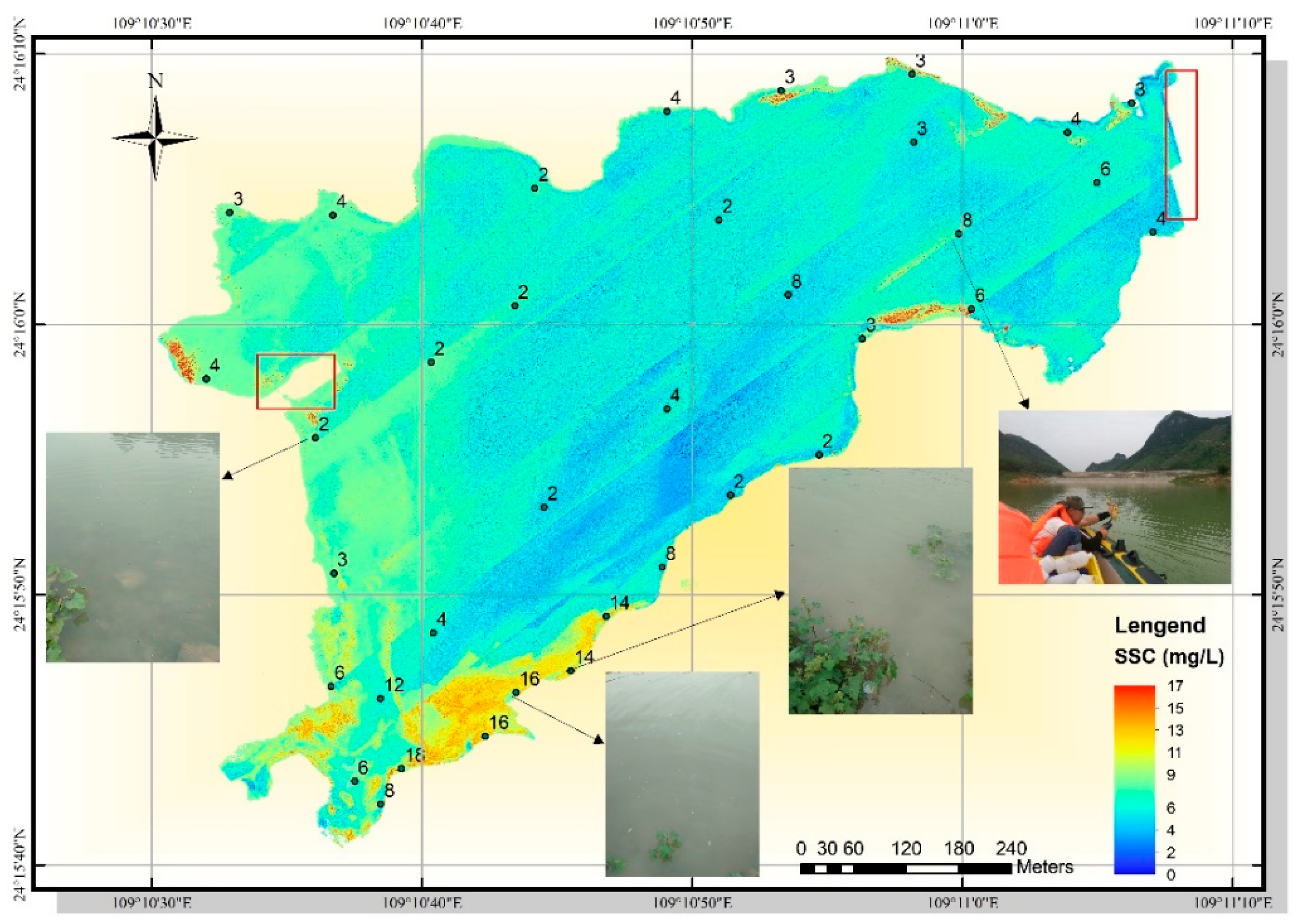
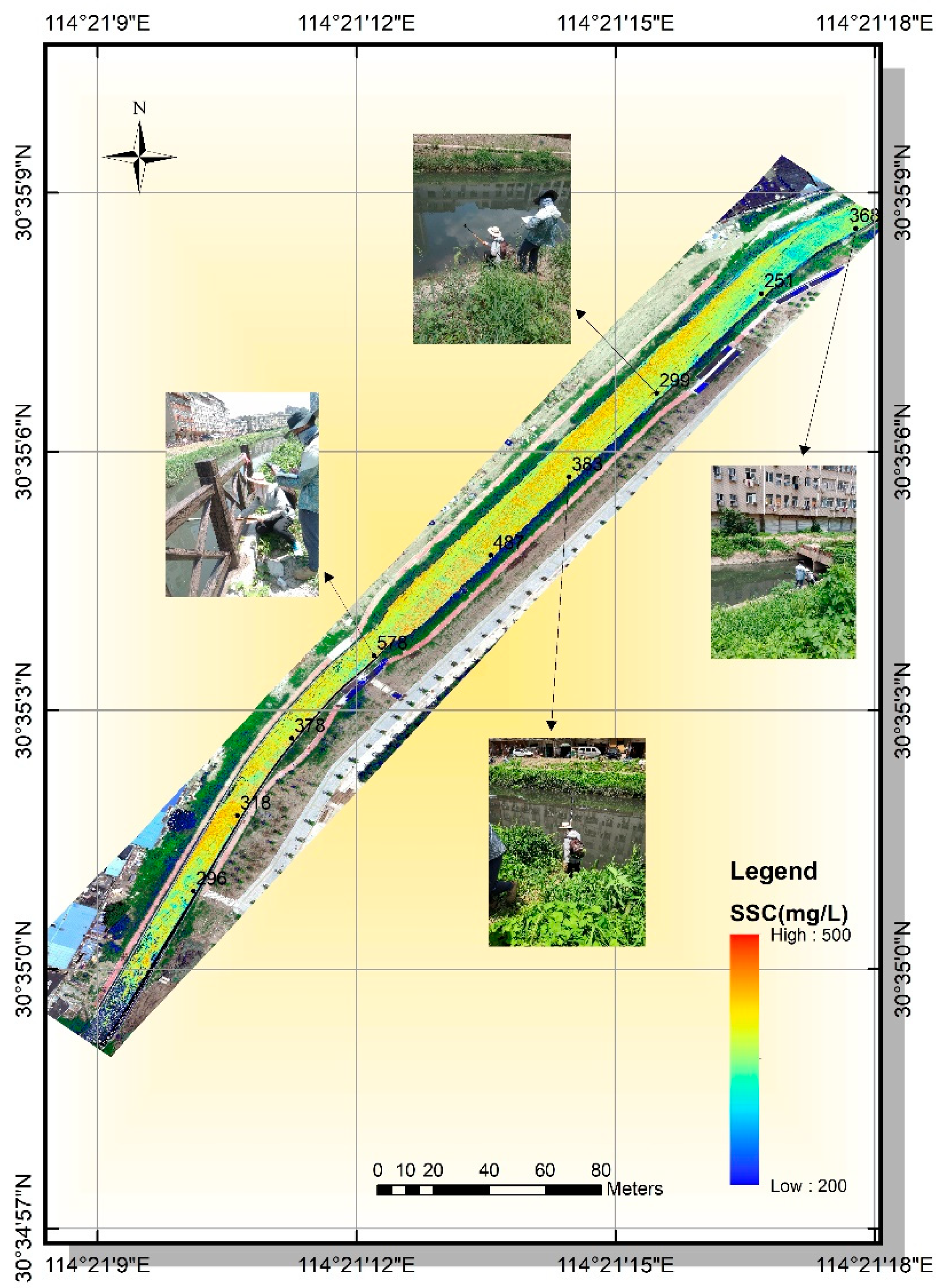
3.5. UAV Image Inversion Based on PSO-LSSVM

Figure 13 shows the results of the inversion of SSC for the UAV-borne HRS images using the PSO-LSSVM algorithm. Due to some problems with the GPS information of the ground control points, some of the edge regions of the spliced image after the geometric correction still cannot be completely overlapped (the area of the red frame). However, the site radiation correction was based on the average position of the 5 × 5 window spectra extracted from the empirical position, so as to minimize the influence of positional deviation between the aerial double-high image pixels and the ground-measured points. In addition, there is a noticeable strip-like chromatic aberration on the image, which is due to the splicing of multiple UAV-borne strip images. Therefore, the inversion results shown only reflect the trend of the SSC distribution in the reservoir, and the prediction results at individual pixel points are not considered here.

According to the inversion results, the maximum SSC in the reservoir is 16.92 mg/L, and the lowest is 0.81 mg/L, which is consistent with the laboratory test results ($SS{C}_{\max }$ = 18 mg/L, $SS{C}_{\min }$ = 2 mg/L). The points marked on Figure 13 are the actual values of SSC at the sampling points.

Further observations are shown in Figure 13. The predicted SSC for the remote sensing imagery is consistent with the observed results in the field. The suspended solids in the southwest part of BR are regionally clustered, and the overall color is close to red. The predicted concentration of suspended solids is above 14 mg/L in this area, which is the highest in the whole reservoir. From Figure 1 (sampling distribution map), the samples collected in the red area are samples 2–6, which are completely consistent with the results shown in Figure 5 (actual measured SSC curve). The measured concentration in this area is 14–18 mg/L. During the field sampling, it was found that a large amount of white foam floated on the surface of the water where the water pollution was serious.

In addition, the inversion image shows that the SSC near the shore is generally high, at about 8 mg/L. In particular, many areas near the shore in the eastern part of the reservoir appear as small-scale red areas. The SSC toward the center of the lake decreases significantly, and is mostly around 2 mg/L. This is due to the human and animal activities along the shore, which result in increased turbidity near the shore. However, the area near the lake center is quiet, with few external disturbances, resulting in low SSC.

In the second experiment, we used the established model to retrieve the UAV-borne HRS images from a riverway in SP, as shown in Figure 14. The points marked on the figure are the actual values of SSC at the sampling points. According to the legend, there is higher SSC in the first half of the riverway, i.e., sampling points 1–5. The average laboratory concentration reaches 411.4 mg/L. The SSC in the second half of the riverway is around 300 mg/L, which is consistent with the laboratory test results of the sample points. It is speculated that the difference of SSC distribution in the riverway may be caused by the different flow direction and width of the riverway. The water flowed from the southwest to the northeast. The initial point passed through a polluted area, which led to increased SSC. Later, due to the widening of the riverway and the precipitation of particulate matter insoluble in water, SSC in the later section decreases. In addition, a clear black area is visible on the edge of the channel on the image. Compared with the original image, it is found that the area is extracted by NDWI and is indeed the water. However, due to the sun’s oblique illumination, the edge of the water is covered by the shadow, and the remote sensing reflectance is low. Therefore, when the experimenter collects the ground-measured spectra, it should try to avoid the shadow area. The gray at the beginning of the river is due to the serious exposure caused by UAV photography, which results in the image masking effect.

4. Conclusions

In this paper, we have described the experimental process of inverting SSC in a water source based on UAV-borne HRS images. Compared with the traditional exponential model, linear model, and the widely used RF algorithm, the estimation accuracy is significantly improved after optimizing the LSSVM model through the widely used PSO algorithm. Moreover, the results of the UAV-borne image inversion were very good. Especially on the HRS images of BR, the distribution of the suspended solids was basically the same as the actual situation, i.e., high concentrations near the shore, low concentrations in the center of the lake, and regional accumulation of suspended solids.

At present, there are few applications in the field of inland water monitoring using UAV-borne hyperspectral data. It is also important to choose the right algorithm for inland water quality monitoring research. It is hoped that the experimental process described in this paper will provide some reference for future research. However, there is still some room for improvement. Although random selection for prediction can achieve a very high modeling and verification accuracy, most of the time not every model that is randomly selected for a sample can perform very well. Therefore, in the future, we will attempt to apply more efficient and stable machine learning algorithms for the quality inspection of inland water environments (suspension, chlorophyll a, heavy metals, etc.). The application of UAV-borne HRS images to water environment research will be a promising development direction in the future. Furthermore, achieving a complete process of automated preprocessing of the UAV-borne images will have far-reaching implications.

References

1. AL-Fahdawi, A.A.H.; Rabee, A.M.; Al-Hirmizy, S.M. Water quality monitoring of Al-Habbaniyah Lake using remote sensing and in situ measurements. Environ. Monit. Assess. 2015, 187, 367. [Google Scholar] [CrossRef] [PubMed]
2. Lei, G.; Zhang, Y.; Pan, D.; Wang, D.; Fu, D. Parameter selection and model research on remote sensing evaluation for nearshore water quality. Acta Oceanol. Sin. 2016, 35, 114–117. [Google Scholar] [CrossRef]
3. Doxaran, D.; Lamquin, N.; Park, Y.-J.; Mazeran, C.; Ryu, J.-H.; Wang, M.; Poteau, A. Retrieval of the seawater reflectance for suspended solids monitoring in the East China Sea using MODIS, MERIS and GOCI satellite data. Remote Sens. Environ. 2014, 146, 36–48. [Google Scholar] [CrossRef]
4. Volpe, V.; Silvestri, S.; Marani, M. Remote sensing retrieval of suspended sediment concentration in shallow waters. Remote Sens. Environ. 2011, 115, 44–54. [Google Scholar] [CrossRef]
5. Giardino, C.; Oggioni, A.; Bresciani, M.; Yan, H. Remote Sensing of Suspended Particulate Matter in Himalayan Lakes: A Case Study of Alpine Lakes in the Mount Everest Region. Mt. Res. Dev. 2010, 30, 157–168. [Google Scholar] [CrossRef]
6. Li, D.; Li, M. Research Advance and Application Prospect of Unmanned Aerial Vehicle Remote Sensing System. Geomat. Inf. Sci. Wuhan Univ. 2014, 39, 505–513. [Google Scholar]
7. Zhong, Y.; Wang, X.; Xu, Y.; Wang, S.; Zhang, L. Mini-UAV-Borne Hyperspectral Remote Sensing: From Observation and Processing to Applications. IEEE Geosci. Remote Sens. Mag. 2018, 6, 46–62. [Google Scholar] [CrossRef]
8. Ma, R.; Duan, H.; Tang, J.; Chen, Z. Remote Sensing of Lake Water Environment, 1st ed.; Science Press: Beijing, China, 2010; ISBN 978-7-03-028776-2. [Google Scholar]
9. Giardino, C.; Brando, V.E.; Dekker, A.G.; Strömbeck, N.; Candiani, G. Assessment of water quality in Lake Garda (Italy) using Hyperion. Remote Sens. Environ. 2007, 109, 183–195. [Google Scholar] [CrossRef]
10. Härmä, P.; Vepsäläinen, J.; Hannonen, T.; Pyhälahti, T.; Kämäri, J.; Kallio, K.; Eloheimo, K.; Koponen, S. Detection of water quality using simulated satellite data and semi-empirical algorithms in Finland. Sci. Total Environ. 2001, 268, 107–121. [Google Scholar] [CrossRef]
11. Ahn, Y.H.; Moon, J.E.; Gallegos, S. Development of Suspended Particulate Matter Algorithms for Ocean Color Remote Sensing. Korean J. Remote Sens. 2001, 17, 285–295. [Google Scholar]
12. Gitelson, A.; Garbuzov, G.; Szilagyi, F.; Mittenzwey, K.H.; Karnieli, A.; Kaiser, A. Quantitative remote sensing methods for real-time monitoring of inland waters quality. Int. J. Remote Sens. 1993, 14, 1269–1295. [Google Scholar] [CrossRef]
13. Wang, Z.; Kawamura, K.; Sakuno, Y.; Fan, X.; Gong, Z.; Lim, J. Retrieval of Chlorophyll-a and Total Suspended Solids Using Iterative Stepwise Elimination Partial Least Squares (ISE-PLS) Regression Based on Field Hyperspectral Measurements in Irrigation Ponds in Higashihiroshima, Japan. Remote Sens. 2017, 9, 264. [Google Scholar] [CrossRef]
14. Hafeez, S.; Wong, M.; Ho, H.; Nazeer, M.; Nichol, J.; Abbas, S.; Tang, D.; Lee, K.; Pun, L. Comparison of Machine Learning Algorithms for Retrieval of Water Quality Indicators in Case-II Waters: A Case Study of Hong Kong. Remote Sens. 2019, 11, 617. [Google Scholar] [CrossRef]
15. Singh, K.P.; Basant, N.; Gupta, S. Support vector machines in water quality management. Anal. Chim. Acta 2012, 703, 152–162. [Google Scholar] [CrossRef] [PubMed]
16. Mueller, J.L.; Fargion, G.S.; McClain, C.R.; Mueller, J.L.; Morel, A.; Frouin, R.; Davis, C.; Arnone, R.; Carder, K.; Steward, R.G.; et al. Ocean Optics Protocols for Satellite Ocean Color Sensor Validation, 4th ed.; Radiometric Measurements and Data Analysis Protocols; Goddard Space Flight Space Center: Greenbelt, MD, USA, 2003; Volume III.
17. Watanabe, F.; Alcântara, E.; Rodrigues, T.; Imai, N.; Barbosa, C.; Rotta, L. Estimation of Chlorophyll-a Concentration and the Trophic State of the Barra Bonita Hydroelectric Reservoir Using OLI/Landsat-8 Images. Int. J. Environ. Res. Public Health 2015, 12, 10391–10417. [Google Scholar] [CrossRef] [PubMed]
18. Chen, S.; Han, L.; Chen, X.; Li, D.; Sun, L.; Li, Y. Estimating wide range Total Suspended Solids concentrations from MODIS 250-m imageries: An improved method. ISPRS J. Photogramm. Remote Sens. 2015, 99, 58–69. [Google Scholar] [CrossRef]
19. Gong, C.L.; Yin, Q.; Kuang, D.B. Correlations Between Water Quality Indexes and Reflectance Spectra of Huangpujiang River. J. Remote Sens. 2006, 10, 910–916. [Google Scholar]
20. Rinnan, Å.; Berg, F.V.D.; Engelsen, S.B. Review of the most common pre-processing techniques for near-infrared spectra. Trends Anal. Chem. 2009, 28, 1201–1222. [Google Scholar] [CrossRef]
21. Rundquist, D.C.; Han, L.; Schalles, J.F.; Peake, J.S. Remote Measurement of Algal Chlorophyll in Surface Waters: The Case for the First Derivative of Reflectance Near 690 nm. Photogramm. Eng. Remote Sens. 1996, 62, 195–200. [Google Scholar]
22. Zhang, M. Spectral indices for estimating ecological indicators of karst rocky desertification. Int. J. Remote Sens. 2010, 31, 2115–2122. [Google Scholar]
23. Pulliainen, J.; Kallio, K.; Eloheimo, K.; Koponen, S.; Servomaa, H.; Hannonen, T.; Tauriainen, S.; Hallikainen, M. A semi-operative approach to lake water quality retrieval from remote sensing data. Sci. Total Environ. 2001, 268, 79–93. [Google Scholar] [CrossRef]
24. Cortes, C.; Vapnik, V. Support-vector networks. Mach. Learn. 1995, 20, 273–297. [Google Scholar] [CrossRef]
25. Suykens, J.; Vandewalle, J. Least Squares Support Vector Machine Classifiers. Neural Process. Lett. 1999, 9, 293–300. [Google Scholar] [CrossRef]
26. Ismail, S.; Shabri, A.; Samsudin, R. A hybrid model of self-organizing maps (SOM) and least square support vector machine (LSSVM) for time-series forecasting. Expert Syst. Appl. 2011, 38, 10574–10578. [Google Scholar] [CrossRef]
27. Yan, Z.G. The PSO-LSSVM model for predicting the failure depth of coal seam floor. In Proceedings of the Intelligent Control & Automation, Beijing, China, 6 July 2012. [Google Scholar]
28. Kennedy, J.; Eberhart, R. Particle swarm optimization. Proc. IEEE Int. Conf. Neural. Netw. Piscataway. IEEE Serv. Cent. 1995, 12, 1941–1948. [Google Scholar]
29. Eberhart, R.C.; Shi, Y. Particle swarm optimization: Developments, applications and resources. In Proceedings of the Congress on Evolutionary Computation, Wellington, New Zealand, 10 June 2002. [Google Scholar]
30. Eberhart, R.C.; Shi, Y. Comparison between genetic algorithms and particle swarm optimization. In Proceedings of the International Conference on Evolutionary Programming, Berlin, Germany, 1998. [Google Scholar]
31. Zhu, X.L.; Xiong, W.L.; Xu, B.G. A Particle Swarm Optimization Algorithm Based on Dynamic Intertia Weight. Comput. Simul. 2007, 24, 154–157. [Google Scholar]
32. Kumar, D.N.; Janga Reddy, M. Multipurpose Reservoir Operation Using Particle Swarm Optimization. J. Water Resour. Plan. Manag. 2007, 133, 192–201. [Google Scholar]
33. Sedki, A.; Ouazar, D. Hybrid particle swarm optimization and differential evolution for optimal design of water distribution systems. Adv. Eng. Inform. 2012, 26, 582–591. [Google Scholar] [CrossRef]
34. Kallio, K.; Koponen, S.; Ylöstalo, P.; Kervinen, M.; Pyhälahti, T.; Attila, J. Validation of MERIS spectral inversion processors using reflectance, IOP and water quality measurements in boreal lakes. Remote Sens. Environ. 2015, 157, 147–157. [Google Scholar] [CrossRef]
35. Han, L.; Rundquist, D.C. The response of both surface reflectance and the underwater light field to various levels of suspended sediments: Preliminary results. Photogramm. Eng. Remote Sens. 1994, 60, 1463–1471. [Google Scholar]
36. Berthon, J.F.; Zibordi, G. Optically black waters in the northern Baltic Sea. Geophys. Res. Lett. 2010, 37, 232–256. [Google Scholar] [CrossRef]
37. Duan, H.; Ma, R.; Loiselle, S.A.; Shen, Q.; Yin, H.; Zhang, Y. Optical characterization of black water blooms in eutrophic waters. Sci. Total Environ. 2014, 482–483, 174–183. [Google Scholar] [CrossRef] [PubMed]
38. Doxaran, D.; Froidefond, J.M.; Lavender, S.; Castaing, P. Spectral signature of highly turbid waters: Application with SPOT data to quantify suspended particulate matter concentrations. Remote Sens. Environ. 2002, 81, 149–161. [Google Scholar] [CrossRef]
Figure 1. Sampling sites at Beigong Reservoir (BR) in Liuzhou.
Remotesensing 11 01455 g001
Figure 2. Sampling sites at the polluted riverway Shahu Port (SP) in Wuhan.
Remotesensing 11 01455 g002
Figure 3. Preprocessing of the UAV-borne HRS images and extracted hyperspectral data.
Remotesensing 11 01455 g003
Figure 4. The 36 spectral curves extracted from the UAV-borne HRS images after the preprocessing.
Remotesensing 11 01455 g004
Figure 5. Results of the SSC laboratory testing.
Remotesensing 11 01455 g005
Figure 6. Pearson’s correlation coefficients with suspended solids concentration: (a) Original spectra. (b) Max-min normalization result. (c) First-order derivative result. (d) Continuum removal result. (e) Band ratio result.
Remotesensing 11 01455 g006aRemotesensing 11 01455 g006b
Figure 7. The 29 spectral curves extracted from the UAV-borne HRS images after the preprocessing.
Remotesensing 11 01455 g007
Figure 8. Results of the SSC laboratory testing.
Remotesensing 11 01455 g008
Figure 9. Pearson’s correlation coefficients with suspended solids concentration: (a) Original spectra. (b) Max-Min normalization result. (c) First-order derivative result. (d) Continuum removal result. (e) Band ratio result.
Remotesensing 11 01455 g009aRemotesensing 11 01455 g009b
Figure 10. Flow diagram of PSO-LSSVM for the inversion of suspended solids concentration.
Remotesensing 11 01455 g010
Figure 11. Fitness curve of PSO optimization: (a) BR; and (b) SP.
Remotesensing 11 01455 g011
Figure 12. Relationship between the predicted and measured values of suspended solids concentration: (a) BR; and (b) SP.
Remotesensing 11 01455 g012
Figure 13. Inversion results of SSC for the UAV-borne HRS images for the BR dataset.
Remotesensing 11 01455 g013
Figure 14. Inversion results of SSC for the UAV-borne HRS images for the SP dataset.
Remotesensing 11 01455 g014