Article

The Comparison of Fusion Methods for HSRRSI Considering the Effectiveness of Land Cover (Features) Object Recognition Based on Deep Learning

1
School of Geomatics and Urban Spatial Information, Beijing University of Civil Engineering and Architecture, Beijing 100044, China
2
Key Laboratory for Urban Geomatics of National Administration of Surveying, Mapping and Geoinformation, Beijing 100044, China
*
Author to whom correspondence should be addressed.
Remote Sens. 2019, 11(12), 1435; https://doi.org/10.3390/rs11121435
Submission received: 21 May 2019 / Revised: 11 June 2019 / Accepted: 13 June 2019 / Published: 17 June 2019
(This article belongs to the Special Issue Remote Sensing based Building Extraction)

Abstract

:
The efficient and accurate application of deep learning in the remote sensing field largely depends on the pre-processing technology of remote sensing images. Particularly, image fusion is the essential way to achieve the complementarity of the panchromatic band and multispectral bands in high spatial resolution remote sensing images. In this paper, we not only pay attention to the visual effect of fused images, but also focus on the subsequent application effectiveness of information extraction and feature recognition based on fused images. Based on the WorldView-3 images of Tongzhou District of Beijing, we apply the fusion results to conduct the experiments of object recognition of typical urban features based on deep learning. Furthermore, we perform a quantitative analysis for the existing pixel-based mainstream fusion methods of IHS (Intensity-Hue Saturation), PCS (Principal Component Substitution), GS (Gram Schmidt), ELS (Ehlers), HPF (High-Pass Filtering), and HCS (Hyper spherical Color Space) from the perspectives of spectrum, geometric features, and recognition accuracy. The results show that there are apparent differences in visual effect and quantitative index among different fusion methods, and the PCS fusion method has the most satisfying comprehensive effectiveness in the object recognition of land cover (features) based on deep learning.

Graphical Abstract

1. Introduction

With the development of earth observation technology, a large number of remote sensing satellites have been launched, which further improves the acquisition ability of high spatial resolution and high spectral resolution imagery, and provides extensive data sources for applications [1]. Object recognition of urban typical land features from High Spatial Resolution Remote Sensing Imagery (HSRRSI) is an active and important research task driven by many practical applications. Traditional methods are based on hand-crafted or shallow-learning-based features with limited representation power [2].
In recent years, the application of deep learning in the field of remote sensing has become more and more extensive, and its progress has solved many problems, especially in target detection [3], target recognition [4], and semantic segmentation [5], which has taken the current research to a new height. High spatial resolution remotely sensed imagery often contains multiple types of land-cover with distinct spatial, spectral, and geometric characteristics, and the manual labeling sample is not enough, which limits the applications of deep learning in object recognition from HSRRSI [6].
Over the last decades, a number of relevant methods have been proposed by combining the spatial and the spectral information to extract spatial–spectral features [7,8,9,10,11,12,13,14,15,16,17,18,19]. In a recent study, Cheng propose a unified metric learning-based framework to alternately learn discriminative spectral-spatial features; they further designed a new objective function that explicitly embeds a metric learning regularization term into SVM (Support Vector Machine) training, which is used to learn a powerful spatial–spectral feature representation by fusing spectral features and deep spatial features, and achieved state-of-the-art results [20]. It is now commonly accepted that spatial–spectral-based methods can significantly improve the classification performance, which also reflects the importance of spatial and spectral features of image data in application-level in deep learning. However, the number of labeled samples in HSRRSI is quite limited because of the high expense of manually labeling, and even the available labels are not always reliable. Making full use of HSRRSI to produce high-quality training data will be a challenge.
The Worldview-3 images used in this study are composed of the panchromatic band and multispectral bands. The former has high spatial resolution and the latter has high spectral resolution. The questions remains of how to effectively utilize these remote sensing image data and take them as a whole to the greatest extent for comprehensive analysis and application. Spatial–spectral fusion can solve the constraints between spatial resolution and spectral resolution. In the processing stage, remote sensing images with different spatial and spectral resolutions in the same region are fused to obtain images with both high spatial resolution and high spectral resolution. Panchromatic-multispectral fusion is the most classical method of spatial–spectral fusion and the first choice for various applications. The fusion technology originated in the 1980s [21,22,23]. Since the SPOT-1 satellite system first provided panchromatic and multispectral images simultaneously in 1986, panchromatic-multispectral fusion technology has developed rapidly; a lot of methods have been proposed [24,25,26].
In general, the existing mainstream panchromatic and multispectral fusion methods can be divided into four categories: component substitution-based fusion [27,28], multi-resolution analysis-based fusion [29,30], model optimization-based fusion [31,32], and sparse expression-based fusion methods [33]. Although there are many existing fusion methods, it is still challenging to find a suitable image fusion method for specific data sources and specific application scenarios.
In this study, six traditional spatial–spectral fusion methods are selected for panchromatic and multispectral bands in the study area to generate remote sensing images with both high spatial resolution and high spectral resolution. Then, we apply image fusion results to conduct the experiments of land cover (features) object recognition for remote sensing images based on Mask R-CNN [34]. The experimental results demonstrate the effectiveness of the proposed method and reveal the potential application of image fusion technology in target recognition and feature-oriented primitive processing, analysis, and understanding. By comparing the recognition results of different fusion methods, we obtain a fusion image that is more suitable for network generalization ability. It also verifies that a fusion image with high spatial resolution and high spectral resolution achieves better recognition effect.

2. Methodology

2.1. Image Fusion Methods

In order to improve the quality of remote sensing image data, such as resolution, contrast, integrity, and other indicators, various fusion methods have been developed. The common methods are IHS (Intensity-Hue Saturation), PCS (Principal Component Substitution), ELS (Ehlers) [35,36], GS (Gram Schmidt), HPF (High-Pass Filtering) [21], and HCS (Hyper spherical Color Space). In this study, we use these six methods to evaluate the adaptability of six fusion methods to high-resolution imagery and their effectiveness of land cover (features) object recognition based on deep learning.
IHS transformation can effectively separate spatial (intensity) and spectral (hue and saturation) information from a standard Red-Green-Blue (RGB) image [37]. First, the IHS method transforms an RGB image into the IHS image space. The IHS color space is represented by Intensity (I), Hue (H), and Saturation (S). The effect of this representation of remote sensing images aligns better with human visual habits, making the image objects look more similar to the color changes of real objects, and closer to the human perception mechanism of color. Next, the intensity component (I) is replaced by the panchromatic image. Then, an inverse IHS transformation is performed to obtain a fused image that has high spatial resolution and hyperspectral resolution. The specific process is shown in Figure 1. The fused image obtained by transformation, substitution, and inverse transformation not only has the advantage of high resolution of panchromatic image, but also maintains the hue and saturation of the multispectral image. These characteristics will be beneficial to the subsequent deep learning models to capture the fine features of the complex land-use images used for generalization.
Compared with IHS transformation, the Principal Component Substitution (PCS) technique uses Principal Component Transformation (PCT), with which number of input bands is not limited to three. PCS is a multi-dimensional linear transformation fusion based on image statistical features, which can concentrate variance information and compress data. When using the PCT in image fusion, the first component of the low spatial resolution images is replaced by the high spatial resolution images. The fused images are obtained by applying an inverse PCT on the new set of components [38,39]. This fusion method has a wide range of applications, and the image after inverse transformation of principal components is clearer and richer. It can more accurately reveal the internal structure of multi band remote sensing information data, thereby reducing the difficulty and complexity of the subsequent deep learning feature extraction model. The specific process is shown in Figure 2.
GS fusion method mainly uses Gram–Schmidt Transformation in mathematics, which can effectively eliminate the correlation between multi-spectral bands. It is similar to the Principal Component Transform (PCA) method and is commonly used in mathematics. GS fusion firstly obtains a low-resolution panchromatic image from a multi-spectral image and uses the image as the first band of multi-spectral image to recombine with the original multi-spectral image. Then, GS transformation is applied to the reconstructed multi-band image. Equation (1) is the concrete equation of the GS transformation. The panchromatic image is used to replace the first band of the image after GS transformation. Lastly, the fused image is obtained by GS inverse transformation. GS transformation gives the image higher contrast, and can better maintain the spectral information of the original image with less information distortion. This algorithm can weaken the correlation between multispectral bands, thus reducing information redundancy, highlighting more useful or discriminative information in the data itself, thus increasing the effectiveness of land cover (features) object recognition based on deep learning.
G S T ( i , j ) = ( B T ( i , j ) µ T ) i = 1 T 1 ( ( B T , G S i ) × G S i ( i , j ) µ T = j = 1 N i = 1 M B T ( i , j ) M × N ( B T , G S i ) = [ δ ( B T , G S i ) δ ( G S i , G S i ) 2 ] }
In Equation (1), G S T denotes the T orthogonal component after GS transformation; B T represents the T band of the original low spatial resolution remote sensing image; M and N represent the total number of rows and columns of the image; i and j represent the rows and columns of the original low spatial resolution image, respectively; µ T is the mean of the gray value of pixels in the T band of the original low spatial resolution remote sensing image; ( B T , G S i ) is the covariance between the T band of the original low spatial resolution image and G S i .
The difference between GS and PCA is that the information contained in the PCA is mainly in the first component with the most information, and its information decreases in turn in the remaining color components, while the components transformed by Gram-Schmidt are only orthogonal, and the amount of information contained in each component is not significantly different [40]. Therefore, the GS transform can preserve the spectral information of original multispectral images and the spatial texture features of panchromatic images to the greatest extent, so as to solve the problem of excessive concentration of the first component in PCT. However, the GS transformation is relatively complex and unsuitable for large-scale image fusion.
Both IHS and PCS fusion methods pertain to component substitution methods, which are remarkable image fusion techniques that are able to meet user’s needs in most application scenarios. Insufficiently, the computational complexity of these methods is too high to merge massive volumes of data from new satellite images quickly and effectively. For that reason, many research studies have been carried out to develop an advanced image fusion method with a fast computing capability and to preserve the high spatial and spectral quality [41]. One of the improved standard data fusion techniques is the Ehlers fusion method. The Ehlers fusion algorithm was founded by Professor Manfred Ehlers of the University of Osnabluk. The basic principle of the Ehlers fusion algorithm is to sharpen the panchromatic band by using Fast Fourier Transform (FFT filtering), and then use the IHS transform for image fusion. The advantage of this algorithm is that it provides three preset filtering models for different regional images, which are urban, suburban, and suburban mixed areas, respectively. This feature preserves the same spatial characteristics of the fused image as the original image. The specific process of the ELS fusion method are shown in Figure 3.
High-Pass Filtering is often used in image texture and detailed processing to improve the high-frequency details of images, and highlight the linear features and edge information of images. For a remote sensing image, the spectral information of the image is included in the low-frequency part, and the details, edges, and textures of the image are included in the high-frequency part. The basic principle of High-Pass Filtering (HPF) fusion is to extract the high-frequency part of the image and apply it to the low-resolution image (multi-spectral image) to form the high-frequency feature prominent fusion image [42], which can improve the application accuracy of image target recognition. Equation (1) is the concrete equation of the GS transformation.
H P i = ( W a × M S I i L P ) + ( W b × P A N H P ) ,
In Equation (2), W a and W b are weighted, respectively, and added to 1; M S I i L P represents the result of low-pass filtering of low-resolution image (multi-spectral image) in band i, P A N H P represents the result of high-pass filtering of high-resolution image (panchromatic image), and H P i represents the fusion image of original multi-spectral image in band i after the above processing. This method not only effectively reduces the low-frequency noise in high-resolution images, but also can be used in all multi-spectral bands after filtering.
Hyper spherical Color Sharpening (HCS) is a fusion method suitable for multi-band images. For a remote sensing image with N bands, it is shown as a strength I component and N-1 angle component on the hypersphere. The mathematical function of the fusion of HCS method is shown in Equation (3), in which x i is the i component of the original color space.
I = x 1 2 + x 2 2 + x 3 2 + x n 2 φ 1 = a r c t a n ( x n 2 + x n 1 2 + x n 2 2 + x 2 2 x 1 ) φ n 2 = a r c t a n ( x n 2 + x n 1 2 x n 2 ) φ n = a r c t a n ( x n x n 1 ) }
This method converts multi-band remote sensing data into the hyper spherical color space by constructing models and simulating the panchromatic band I component, so as to obtain a sharpened panchromatic band I component, and finally to reverse the data to obtain the fusion image. The fusion image of this method highlights the edge contour of the object, improves the utilization rate of image information, improves the accuracy and reliability of subsequent computer interpretation, and is conducive to feature extraction and classification recognition of a subsequent deep learning model.
The aforementioned six methods extract the most valuable information from the original image according to their own characteristics and fuse it into high-quality images, which can improve the spatial resolution and spectral resolution of the original image. In the subsequent experiments, for the optimal fusion results, we demonstrate the effectiveness and practicability of the image in land cover (features) object recognition based on deep learning.

2.2. Object Recognition Method based Mask R-CNN

2.2.1. Mask R-CNN Network Architecture

In recent years, deep learning has been applied to remote sensing measurements in replacement of the empirical feature design process by automatically learning multi-level representations [43]. Since 2012, Convolutional Neural Networks (CNN) have been widely used in image classification. Novel CNN structures, such as AlexNet [4], VGGNet [44], GoogLeNet [45], and ResNet [46], have been shown to be remarkable.
Since 2015, a special CNN structure, known as region-based models, which detects objects by predicting a bounding box of each object, have been developed for pixel-wise semantic segmentation and object detection [43]. For example, these region-based models include R-CNN [47], Fast R-CNN [48], Faster R-CNN [49], and Mask R-CNN [34]. In this paper, the most representative Mask R-CNN in the current field is used as the basic model.
Mask R-CNN is a two-stage framework (Figure 4). The first stage scans the image and generates proposals. The second stage classifies proposals and generates bounding boxes and masks. The backbone network of Mask R-CNN is ResNet101 and FPN (Feature Pyramid Networks). ResNet is the champion of the classification task of the ImageNet competition in 2015, which can increase the network depth to hundreds of layers and has excellent performance. FPN utilizes the feature pyramid generated by ResNet to fully fuse the high-resolution and high-semantic information of low-level features of the image and generates feature maps of different scales into RPN (Region Proposal Networks) and ROI (Region of Interest) Align layers by top-down up sampling and horizontal connection processes. RPN is a lightweight neural network that scans images with sliding windows and searches for areas where objects exist. ROI Align is a regional feature aggregation method proposed by Mask-RCNN, which solves the problem of misalignment caused by two quantifications in ROI Pooling operation. After using RoIAlign, the accuracy of the mask is improved from 10% to 50%. Another breakthrough of the model is the introduction of semantic segmentation branch, which realizes the decoupling of the relationship between mask and class prediction. The mask branch only does semantic segmentation, and the task of type prediction is assigned to another branch.

2.2.2. Network Training

As an initial experiment, we trained a Mask R-CNN model on the RSSCN7 Dataset [50] and RSDataset [51]. The pixel resolution of the above dataset is 0.3m. We selected 996 images as training data and 200 images as testing data (Table 1). Several typical landmark, including buildings and water bodies, a=were selected as marking samples (Figure 5). All target objects in training and testing data sets were labeled manually, including attributes and masking information of objects. Figure 6 is the examples of training sample masks of Figure 5.
Based on Tensorflow, keras, and Anaconda deep learning libraries, we use NVIDIA GeForce GTX 1060 with a single GPU to train 996 training data samples (21,757 buildings, 216 water bodies) and generate a recognition model. The total training time is 58 hours. The main parameters of the Mask R-CNN model are set in Table 2. We use the trained model to recognize buildings and water bodies in 200 test data sets, including 3254 buildings and 185 water bodies. Figure 7 and Figure 8 are examples of recognition results of buildings and water bodies, respectively. Table 3 reflects the recognition accuracy. The precision and recall rate of building recognition reached 0.8275 and 0.7828, respectively, and the precision and recall rate of water body recognition reached 0.8529 and 0.9062, respectively, which confirm the availability of the model.

3. Experiment

3.1. Experimental Area

This study chooses the high-resolution remote sensing image data of Tongzhou New Town in Beijing City acquired by Digital globe’s WorldView-3 satellite on September 19, 2017, as the research area, including panchromatic and multispectral images (Figure 9). The longitude and latitude ranges are nwLat = 39°96′, nwLong = 116°63′, seLat = 39°84′, seLong = 116°78′. The image is geometrically corrected to ensure the effect of data fusion. Because cloud cover is only 0.004 when the image of the study area is acquired, there is no atmospheric correction operation. This area contains countryside, residential, cultural, and industrial areas. Various and versatile architecture types of Surface Coverage Elements with different color, size, and usage make it an ideal study area to evaluate the potential of a building extraction algorithm.
In this study, 800 pixels × 800 pixels were selected as the experimental area (Figure 10). The Mask R-CNN algorithm used in this experiment supports three-band images. Generally, the information content of the three bands is sufficient to support the research of land features (cover) recognition. In this study, a 0.3-m panchromatic image and the R, G, and B bands of a 1.24-m multispectral image are fused by six methods. Finally, a 0.3-m true color high resolution remote sensing image is obtained, which is conducive to subsequent artificial visual interpretation and qualitative and quantitative analysis. This experimental area contains trees, houses, roads, grasslands, and water bodies. The types of land cover are diverse to ensure the effectiveness of the experiment.

3.2. Experimental Method

In this study, the model based on Mask R-CNN is used to recognize the typical urban features from the fused high-resolution remote sensing images. This paper compares and evaluates the adaptability of IHS, PCS, GS, ELS, HPF, and HCS fusion methods to the object recognition of surface coverage (elements) based on deep learning from three aspects: visual effect, quantitative analysis, and object recognition accuracy.

3.3. Result and Discussion

3.3.1. Visual Assessment

The results of six fusion methods are shown in 
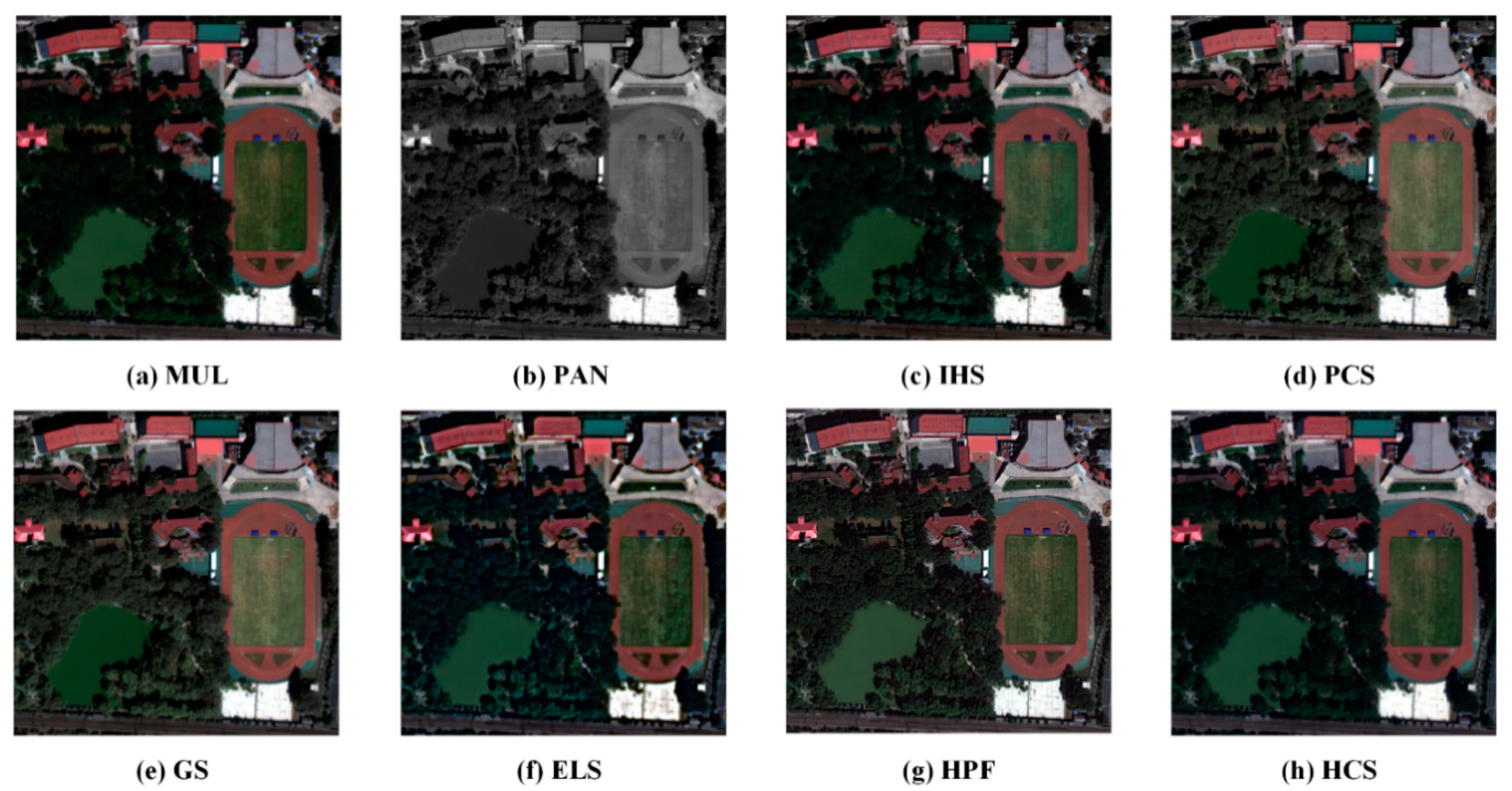
Figure 11. By checking whether the spectral resolution of the fused image is maintained and whether the spatial resolution is enhanced, the quality of the fused image and the adaptability of the method can be evaluated on the whole.
In order to achieve a more detailed visual interpretation effect, this study fuses the images of water, vegetation, roads, playgrounds, and bare land to establish the corresponding atlas (Table 4).
Firstly, we analyze the spectral feature preservation ability of fused images. Compared with the original multispectral image, the fused image basically maintains the spectral characteristics, but there are also significant differences in local color.
The overall color of IHS, PCS, and HCS fusion images is consistent with the original multi-spectral remote sensing image, and the color contrast is moderate. The color of construction land in the GS fusion image is brighter than that of original image combination, and the color of river water changes from grass green to dark green compared with original image combination. After ELS fusion, the brightness of the fused image is darker and the contrast of the image is reduced. After HPF fusion, the edge of the fused image is obvious and the sharpening effect is outstanding.
In terms of spatial information enhancement ability, by comparing the results of the six methods with panchromatic images, we can find that the linear objects, such as roads, water bodies, playgrounds, and residential contours, can be better distinguished and the texture structure of fused images becomes clearer.
PCS, GS, and HPF fusion images have better visual effects, with prominent edges and clear textures of residential areas, roads, playgrounds, water, and woodlands, which are easy to visually interpret. Compared with the three aforementioned methods, IHS and HCS fusion images have some deficiencies in texture clarity of woodland and water bodies, and the other features are very similar in both spectral and spatial characteristics. The ELS transform has serious duplication and blurring phenomena on the boundaries of roads, playgrounds, water, and woodland. In the interlaced area of woodland and architecture, the land features appear inconsistent.
By subjective evaluation of the color, texture structure, clarity, and spatial resolution of the fused image, the quality of the fused image and the superiority of the fusion method can be evaluated as a whole. However, the subtle differences of spectral and spatial characteristics of many fusion images cannot be well distinguished by visual assessment alone. It is necessary to use objective evaluation methods to quantitatively describe the differences between different algorithms.

3.3.2. Quantitative Assessment

This Quantitative evaluation of fusion effect is a complex problem. The objective evaluation method is to determine the statistical parameters of fused images. This method greatly improves the certainty and stability of evaluation.
In this paper, the mean value of each band of the fused image is used to reflect the overall brightness of the image. The main expression is as follows:
µ = 1 M × N i = 1 M j = 1 N F ( i , j ) ,
F (i, j) is the gray value of the fused image F at the pixels (i, j), M and N are the size of image F. The higher the mean value is, the brighter the overall brightness of the image is.
Standard deviation and information entropy are used as quantitative indicators to evaluate image information richness. The standard deviation is obtained indirectly from the mean value, which indicates the degree of dispersion between the gray value and the mean value of the image pixel. The expression of the standard deviation is as follows:
Std = 1 M × N i = 1 M j = 1 N ( F ( i , j ) µ ) 2 ,
The information entropy of fusion image can reflect the amount of image information. Generally, the larger the entropy of the fused image is, the better the fusion quality will be. The calculation equation is as follows:
Ce = i = 0 L P i l o g 2 P i ,
Ce is the information entropy; P i is the occurrence probability of the gray value i of the pixel in the image; L is the maximum gray level of the image.
The definition of the average gradient response image is used to reflect the contrast of minute details and texture transformation features in the image simultaneously. The main expression is as follows:
G = 1 M × N i = 1 M j = 1 N ( ( F ( i , j ) i ) 2 + ( F ( i , j ) j ) 2 ) / 2 ,
Spectral distortion degree is used to evaluate the spectral distortion degree of the fused image relative to the original image. The spectral distortion expression is defined as:
Warp = 1 W i j | V i , j V i , j | ,
W is the total number of pixels in the image, V i , j and V i , j are the gray values of the fused image and the original image (i, j).
The correlation coefficient with each band of the multispectral image and coefficient of correlation between each band of the fused image and panchromatic image are used as quantitative indicators to measure the spectral fidelity (i.e., the degree of preservation of the advantages of the original panchromatic band and the multispectral band in both geometric and spectral information). The related expression is as follows:
Cc = i = 1 M j = 1 N ( F ( i , j ) µ F ) ( A ( i , j ) µ A ) i = 1 M j = 1 N ( F ( i , j ) µ F ) 2 ( A ( i , j ) µ A ) 2 ,
where µ F and µ A represent the average gray level of fusion image and source image, respectively. The larger the correlation coefficient, the more information the fusion image gets from the source image, the better the fusion effect.
Table 5 shows the statistical analysis between different fusion methods. Comparing the brightness information of fused images, we find that PCS has the largest mean value in R and G bands. The values of the two bands are 322.45 and 396.63, respectively. ELS has the largest mean value in the B band with 397.25 values. The brightness information of GS(R band: 313.25; G band: 380.74; B band: 243.82), HPF(R band: 312.58; G band: 379.63; B band: 242.70,) and HCS(R band: 313.43; G band: 381.05; B band: 243.88) is not significantly different from that of the original multispectral image (R band: 313.08; G band: 380.13; B band: 243.20). Compared with other fusion methods, these three methods have more scene reductively.
Firstly, we can evaluate the spatial information of fused images by standard deviation. From the comparative analysis of standard deviation information, the values of PCS, HCS, HPF, and HCS are stable, which are close to or higher than the original multispectral images. It shows that the gray level distribution of the images is more discrete than the original ones, and the amount of image information has increased, among which PCS (R band: 95.694; G band: 167.71; B band: 173.94) has achieved the best results. The standard deviation of IHS (B band: 88.860) and ELS (B band: 82.816) in the B band is small, which indicates that the gray level distribution of the image is convergent and the amount of image information is reduced.
From the information entropy index, the information entropy of each fusion image is close to or higher than that of the original multi-spectral image. The increase of information entropy indicates that the information of each fusion image is richer than that of the pre-fusion image. In the R band, IHS and ELS reached 1.558 and 1.583 above average, respectively. PCS and HCS fusion methods achieve the overall optimal effect in the G (PCS: 1.328; IHS: 1.324) and B bands (PCS: 1.557; IHS: 1.558), indicating that the information richness of PCS and HCS fusion images are higher than that of other fusion images.
From the analysis of the definition (average gradient) of the fused images, the average gradient of the six fusion images in the G and B bands is close to or higher than that of the original multi-spectral images, except for the R band. This shows that the six fusion methods have been enhanced in spatial information, and the expression effect of detailed information is higher. The HPF fusion method performs best in image clarity.
Comparing the spatial correlation coefficients of six fused images with the original color images, we find that PCS(R band: 0.981; G band: 0.983; B band: 0.973) and GS(R band: 0.976; G band: 0.976; B band: 0.978) achieve better results, indicating that the geometric details of fused images are more abundant, and the spatial correlation between the PCS fusion image and the original image is the highest.
The correlation coefficients of images need to consider not only the ability of the processed image to retain the spatial texture details of the original high spatial resolution image, but also the ability of the image to retain spectral characteristics. Comparing the spectral correlation coefficients between the fused image and the original multi-spectral image, we find that the fused image of PCS, GS, HPF, and HCS has a high correlation with the original image, among which the HCS fusion method has the lowest change in spectral information and the strongest spectral fidelity.
From the analysis of spectral distortion degree, the distortion of IHS in the R band and B band is 105.40 and 96.95, respectively, and ELS (R band: 112.68; B band: 165.51) is much higher than other methods. However, in the G band, the distortion of IHS and ELS is 27.602 and 31.553, respectively, while PCS obtained the maximum distortion of all methods of 47.888, which shows that the performance of different methods in different bands is greatly different. Overall, the distortion degree of his (R band: 105.40; G band: 27.602; B band: 96.955), ELS (R band: 112.68; G band: 31.553; B band: 165.51), and PCS (R band: 27.949; G bands: 0.976; B band: 0.978) is too large, which indicates that the distortion degree of image spectra is greater. The spectral distortion of GS, HPF, and HCS fusion methods is small, which indicates that the spectral distortion of fusion images is low, among which HCS (R band: 0.946; G band: 0.973; B band: 0.988) achieves the best effect.

3.3.3. Accuracy Assessment of Objectification Recognition

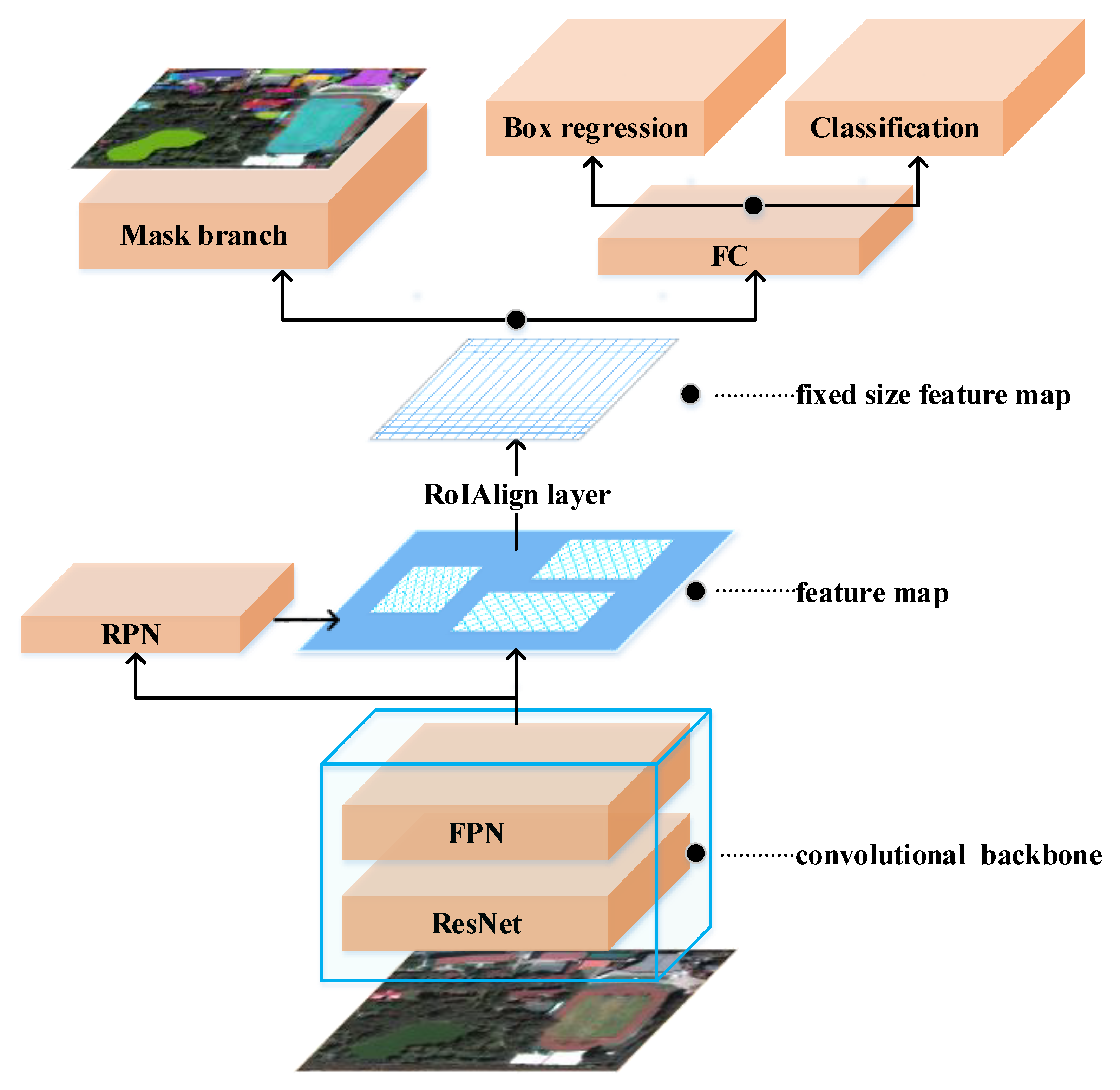
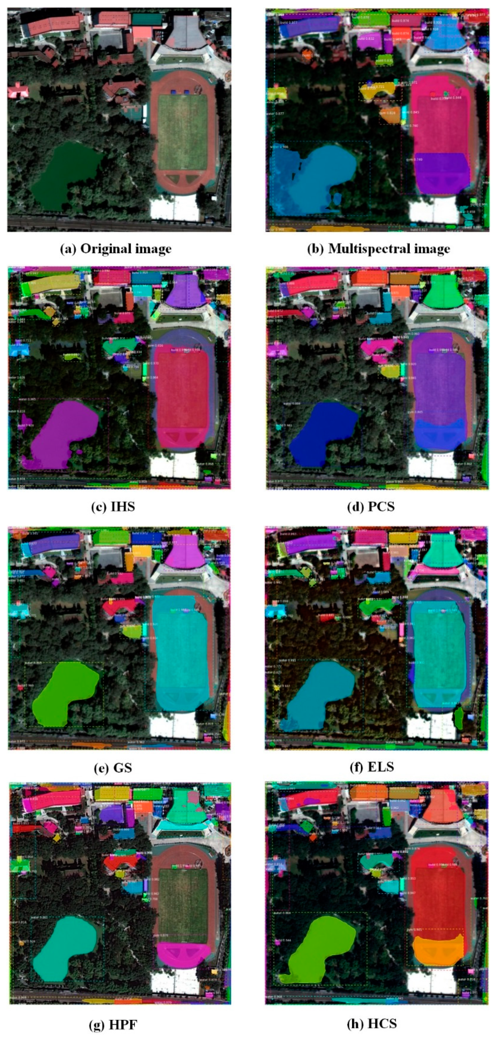
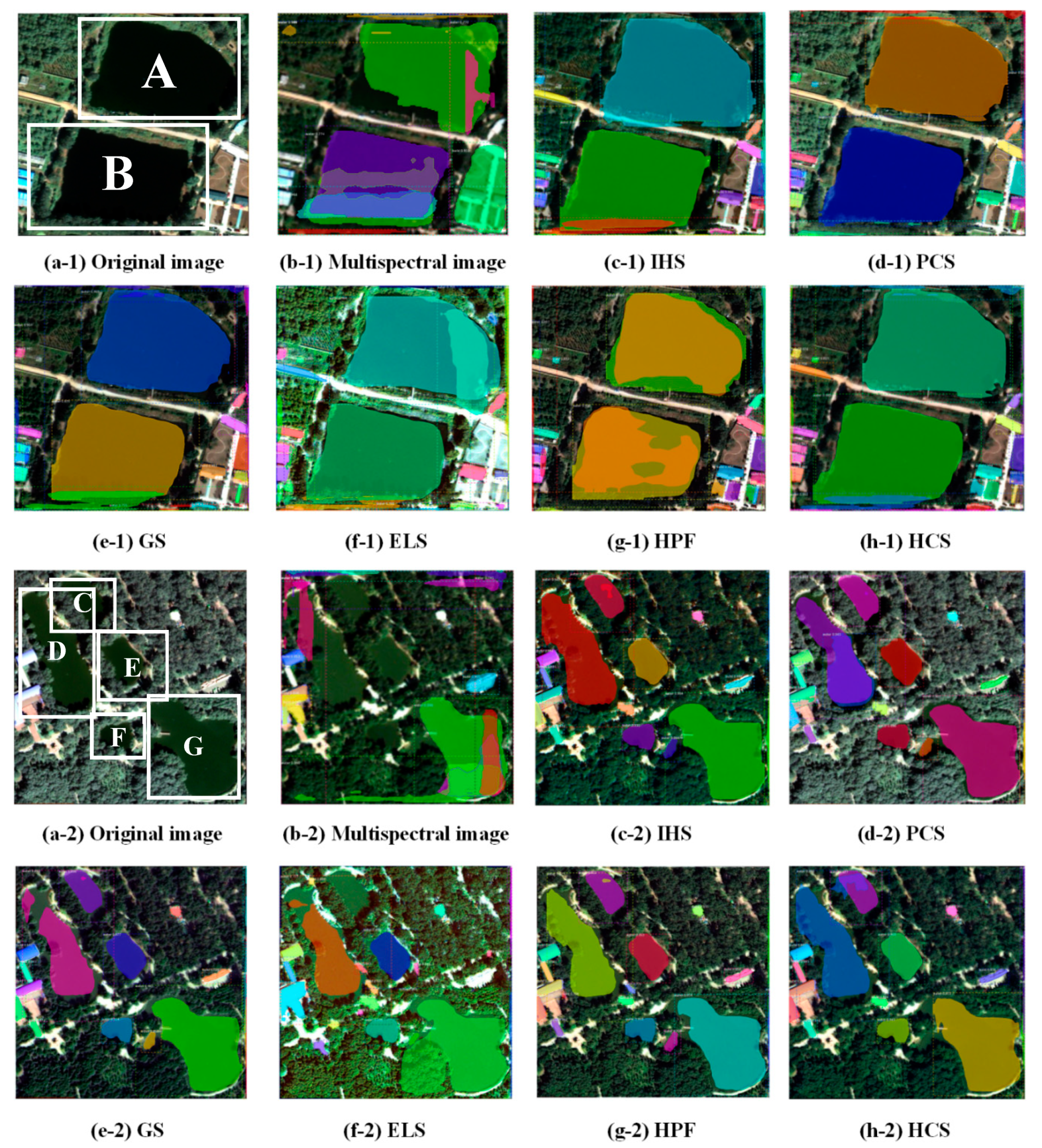
Figure 12 is the recognition result of six fusion methods using the Mask-RCNN model. In Figure 12c–h, the fusion images generated by different fusion methods have different recognition results for buildings, water bodies, and playgrounds. Among them, the overall recognition results obtained by GS and PCS are better, followed by HPF and HCS. The results for IHS and ELS have less satisfying effect.
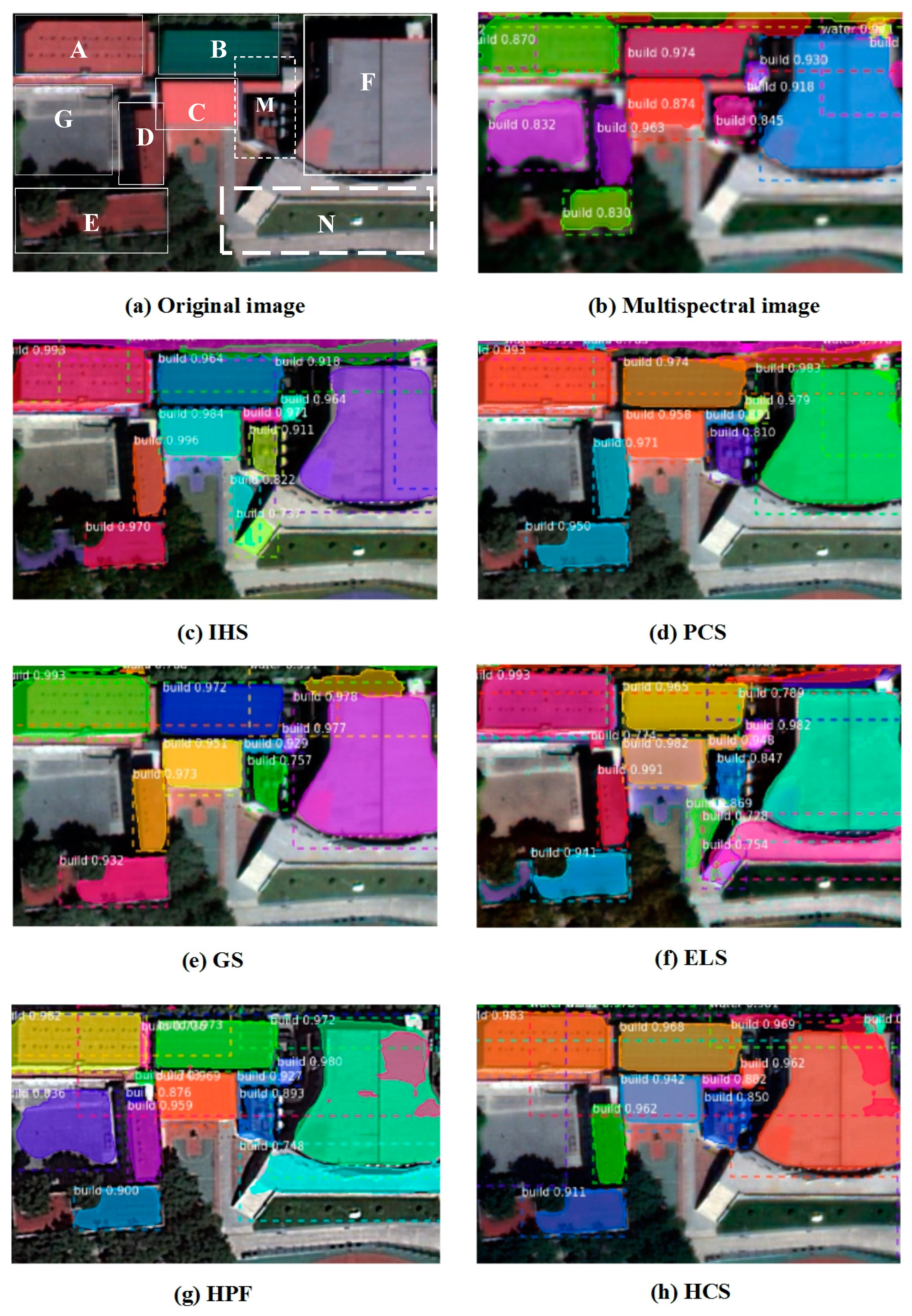
Figure 13 is the recognition result of typical buildings in the fusion image of six methods. The building recognition effect of the left-upper region (Building A, B, C, and D) and right-upper region (Building F), with obvious edge differences, achieves good performance, and almost all of them can be recognized correctly.
The confidence level of object recognition is shown in Table 6. The confidence of PCS in five buildings with clear outlines is the only one of the six methods where all values reach above 0.95. In building A, B, and F, the confidence of PCS is the highest, at 0.933, 0.974, and 0.983, respectively. In building C and D, the confidence of IHS is the highest, at 0.984 and 0.996, respectively. Building E in the lower left area interwoven with vegetation or shadows is shown to be partially unrecognizable. Among the recognition results of building E, the masks based on six fusion methods cannot clearly depict the edges of buildings. The confidence of the recognition results is the lowest among all building individuals. IHS achieves the highest value of 0.970, and PCS achieves confidence of 0.950.
The buildings with small building areas in the middle region (Area M) are easy to be missed due to the interference of spectral characteristics and shadows. Occasionally, buildings with prominent roof structures are misidentified as multiple buildings, resulting in repeated detection. Area N in Figure 13 is composed of stairs and lawns. Except for ELS and HPF, there is no misidentification in other methods. Area G is actually empty space. The HPF method misidentified area N as a building.
Considering the overall effect of building recognition, PCS is the best, achieving more accurate segmentation of building edges, followed by IHS, GS, and HCS, and lastly ELS and HPF, which have different degrees of omission and misidentification.
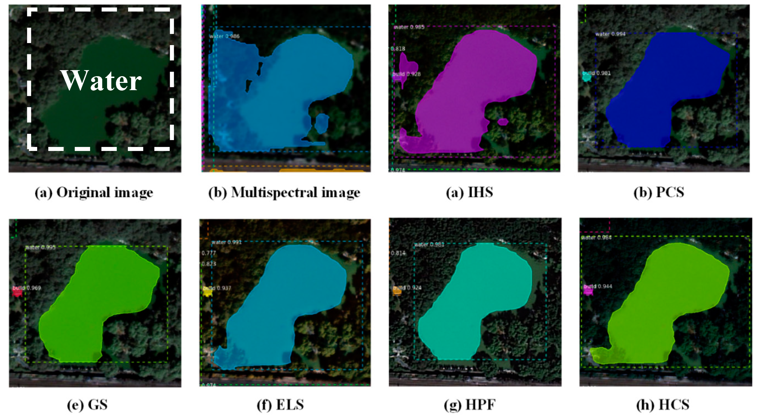
Figure 14 is the result of water body recognition in the fusion image of six methods. PCS, GS, and HPF have better segmentation effect. PCS and GS work better in segmentation of water body edges. The confidence of the two methods is 0.994 and 0.995 (Table 7), respectively. IHS, ELS, and HCS cannot distinguish the confusing parts of water bodies and vegetation shadows.
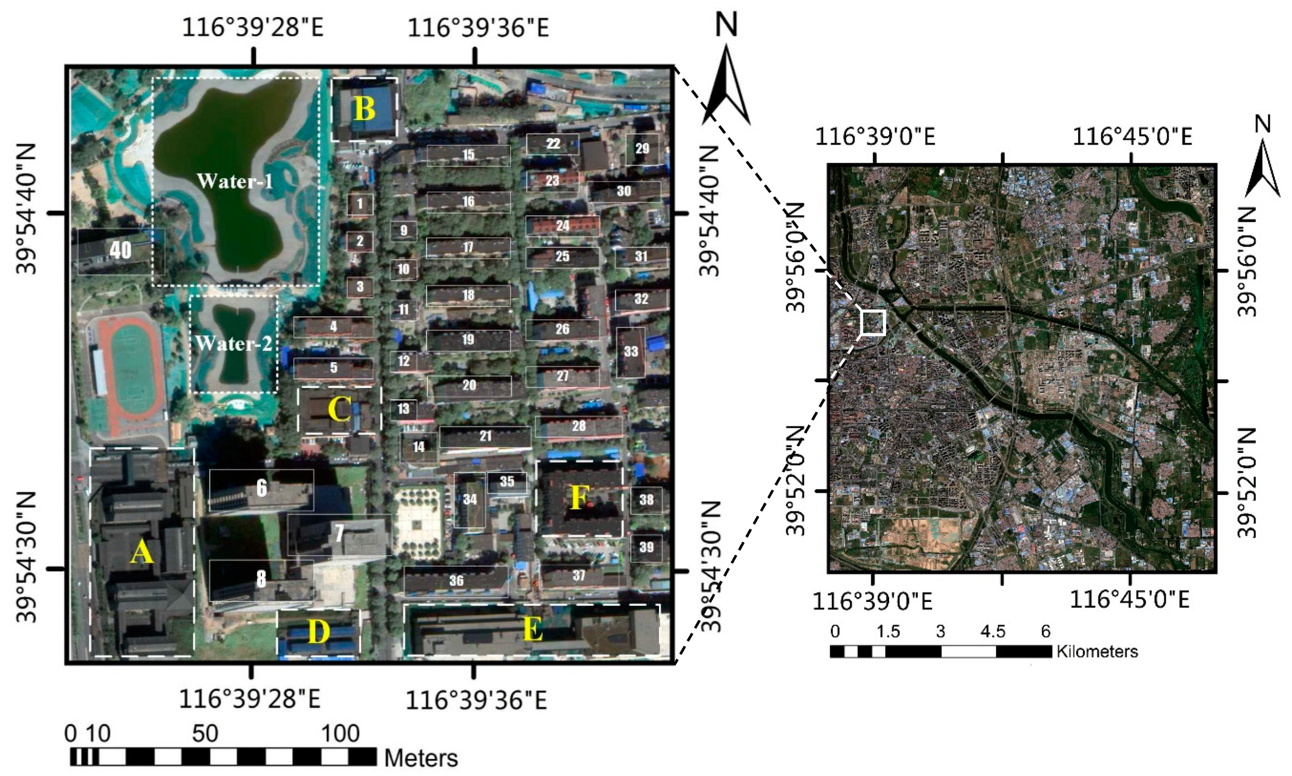
In order to further verify the land cover (features) object recognition efficiency of the model for buildings by using six fusion methods, we selected an experimental area with denser buildings and more building types for building recognition (Figure 15). In total, 50 single buildings in the experimental area were identified by visual interpretation, and six complex building areas were divided for overall analysis.
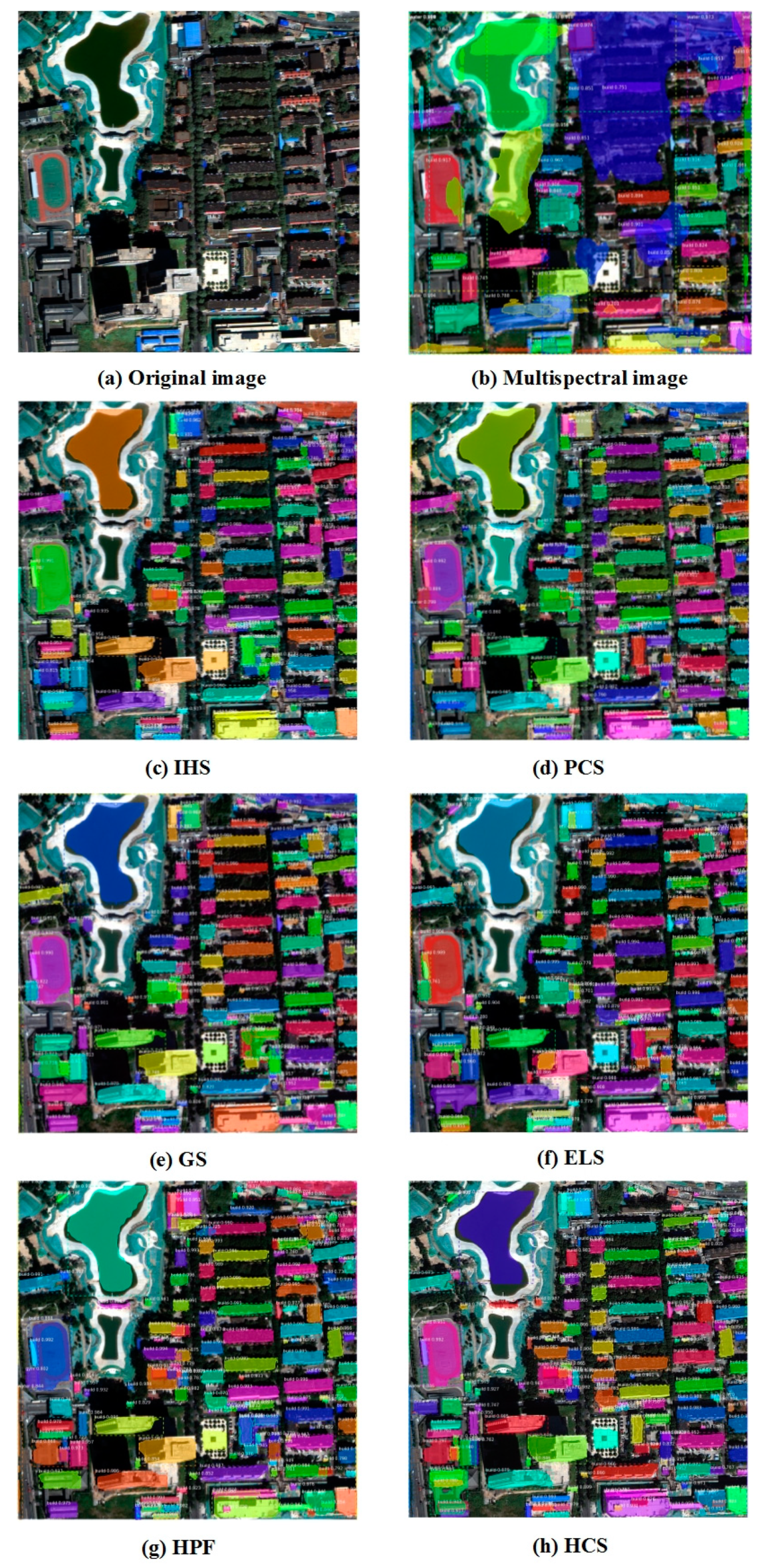
Through the recognition results in Figure 16, we find that the image recognition effect after fusion has been greatly improved. The recognition results of multi-spectral remote sensing images have significant instances of misidentification and omission.
The IHS fusion method missed three buildings, ELS and HPF methods have miss one building. And PCS, GS, and HCS miss no detection. The six methods have achieved effective case segmentation for 40 single buildings. Combined with the data comparison results of Table 8 for confidence level, PCS (0.973) > HCS (0.965) > GS (0.956) > ELS (0.948) > HPF (0.930) > IHS (0.929), we can conclude that the PCS method achieves the best results. Through the recognition results of complex building areas, we find that multi-spectral remote sensing images are recognized as blurred edge masks, which cannot distinguish building units. A–F regions are irregular composite buildings. The recognition results of six fusion images show different degrees of fragmentation, which also provides a breakthrough point for our subsequent training of neural networks and the transformation of the network structure.
In order to further quantitatively evaluate the recognition effect, we evaluate the detection accuracy of buildings in the experimental area by calculating precision and recall. Table 9 shows the results of six fusion methods and multispectral imagery. PCS achieves precision of 0.86 and recall of 0.80. These two indicators are the highest in the six methods. The precision of the multispectral image is only 0.48 and the recall is only 0.197, which also proves that image fusion can significantly improve the effectiveness of object recognition based on deep learning.
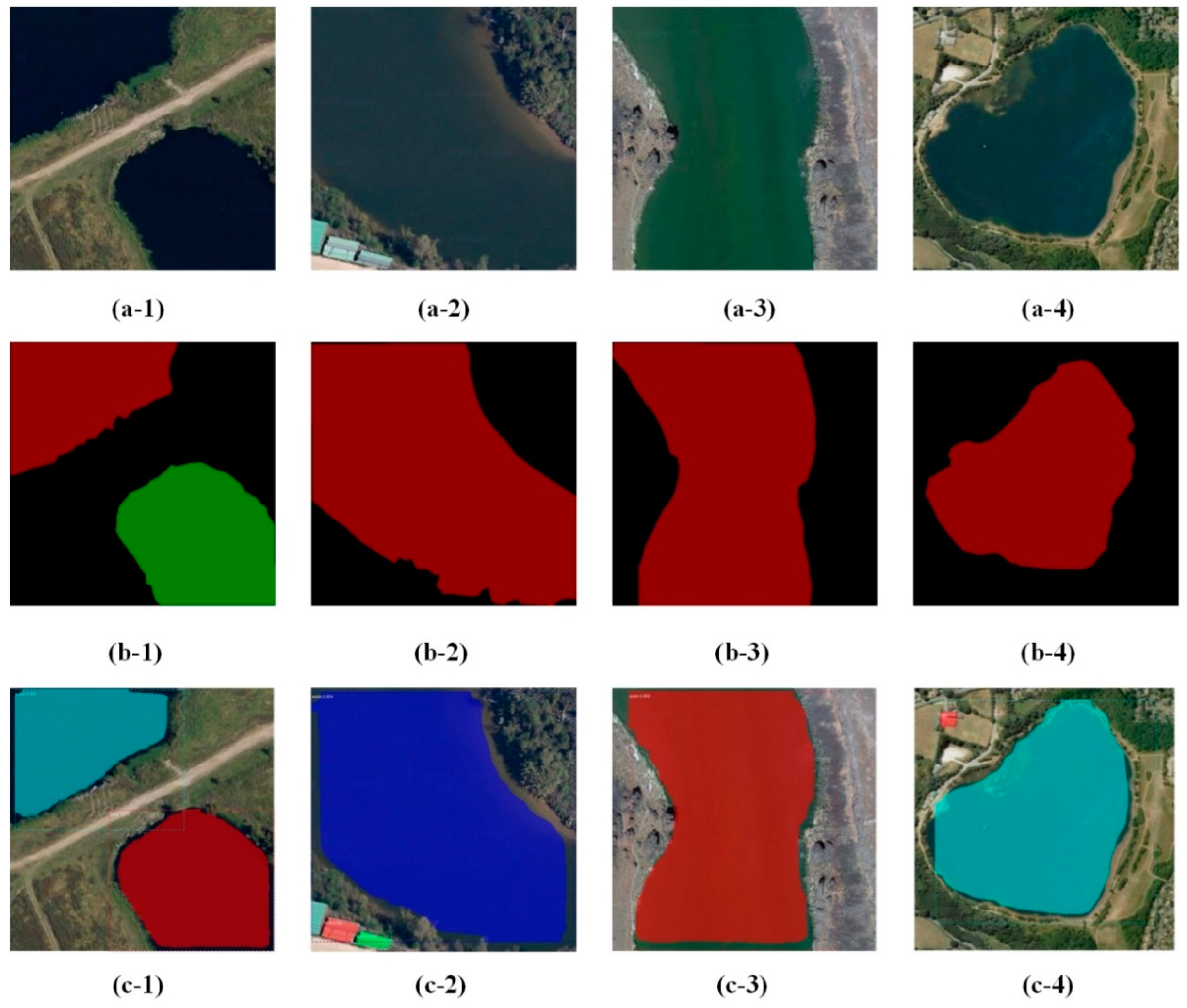
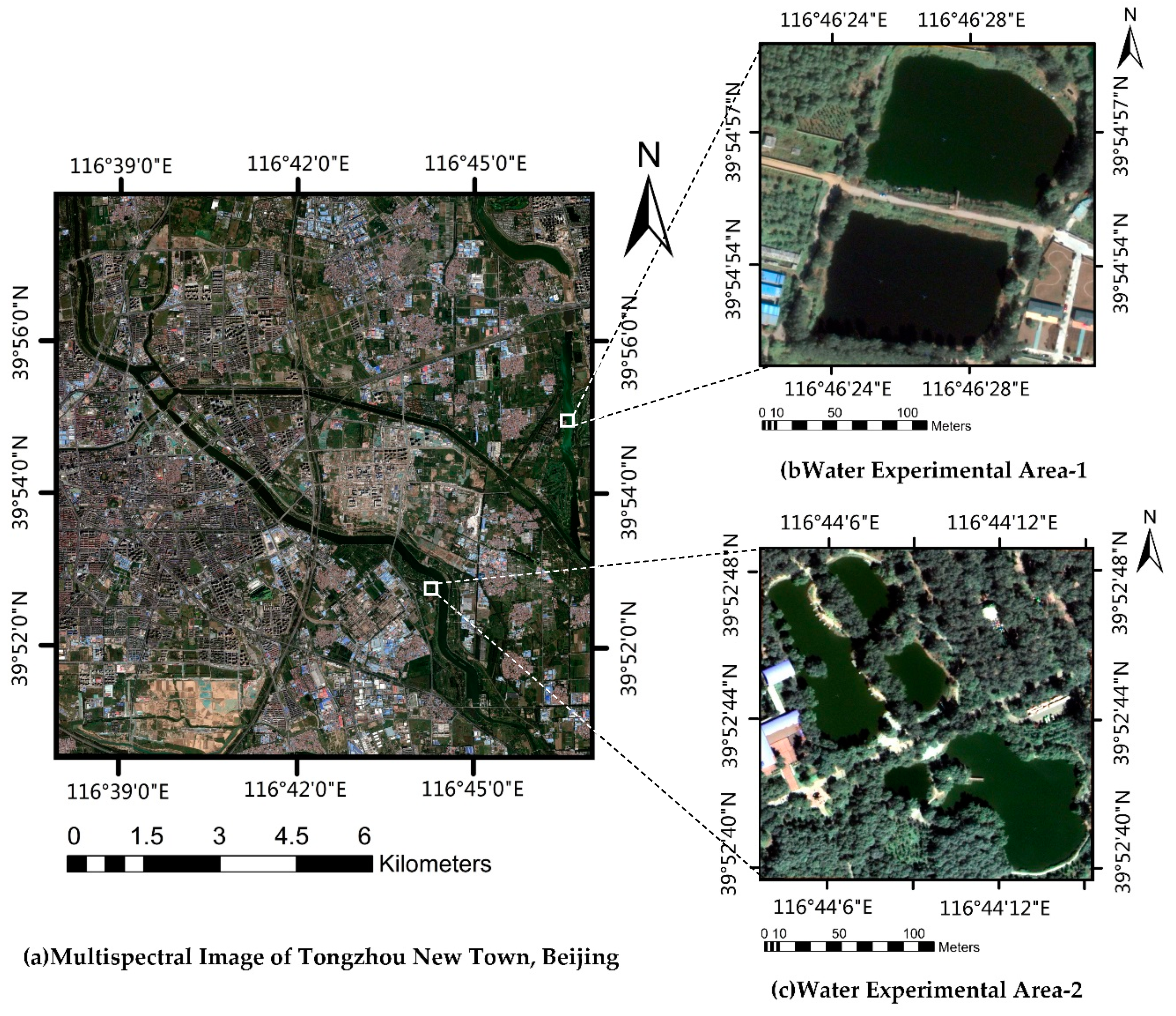
In addition, we selected two experimental areas (Figure 17) with similar and scattered water bodies to further verify the recognition efficiency of water bodies in the image generated by six fusion methods. The water bodies in the selected experimental area are different in size. Dense vegetation and shadows are interlaced with water bodies, which are liable to cause confusion.
Through the recognition results of Figure 18, we find that in the multispectral remote sensing image, the edges of water bodies in regions A and B are significantly confused with vegetation, and the green space is mistaken for a water body. There is a serious missing detection phenomenon in regions C–G. Compared with this, the recognition results of six fusion methods have been greatly improved. PCS can better distinguish the confusing parts of water bodies and vegetation shadows. PCS has the best edge segmentation effect. There is no large area of water missing or overflowing in the segmentation mask. Table 10 shows the data comparison of confidence level, PCS (0.982) > GS (0.944) > HCS (0.934) > IHS (0.931) > HPF (0.904) > ELS (0.767), combined with the water detection results of six fusion methods and multispectral imagery from Table 11, we conclude that PCS has the best effect.
Table 12 reports the computation times of our proposed methods on three experimental areas (experimental area-1, water experimental area-1 and area-2). Combined with detection results in Table 9 and Table 11, we can conclude that the computing time is proportional to detection of objects. How to achieve the balance of efficiency and effect through the improvement of the algorithm is the next important research direction.
From the above experiments, we can draw a conclusion that the object recognition method based on Mask-RCNN applied in this paper can recognize objects. The image recognition effect for two types of objects largely varies with different fusion methods, and the overall effect of PCS and GS is better. It is noteworthy that there is a common phenomenon in the results of object recognition. The segmentation effect of the edge of the mask is not satisfying, and the edge of the mask cannot be fully fitted to the object for segmentation. In the subsequent sample making and model improvement, the segmentation effect of the edge of the object needs to be further optimized.

4. Conclusions

Image fusion is the fundamental way to realize the complementary advantages between the high spatial resolution of the panchromatic band and the high spectral resolution of multispectral bands. In the pretreatment of model training data, we compared six fusion methods, IHS, PCS, GS, ELS, HPF, and HCS, by applying them to the same WorldView-3 satellite image. The results show that the fusion images obtained by different fusion methods are very different in visual effect and quantitative index.
Land cover (features) recognition effectiveness for buildings and water bodies using six fusion methods are notably different, and the recognition accuracy has been significantly improved compared with the original multi-spectral remote sensing images. Considering the subsequent segmentation and feature-oriented primitive processing, analysis, and understanding, PCS fusion method has the best comprehensive effect.
We use deep learning to perform typical object recognition of land cover (features) in remote sensing images, but there is still a long way to go to meet the standards of surveying and mapping products. Realizing the automation from remote sensing image to sematic vector map production is the ultimate goal. Compared with the object instance segmentation based on Mask-RCNN, the extraction of building vector contours based on instance segmentation will be more challenging in the current research field.

Author Contributions

The following contributions were given to this research effort: Conceptualization, S.S.; Methodology, S.S., and H.P.; Software, S.S.; Validation, S.S., Y.L. and H.P.; Formal analysis, S.S.; Investigation, H.P.; Resources, S.S.; Data curation, Y.L.; Writing—original draft preparation, S.S.; writing—review and editing, J.L.; Visualization, J.L.

Funding

This research is funded by National Natural Science Foundation of China (No. 41301489), Beijing Natural Science Foundation (No.4192018, No. 4142013), Outstanding Youth Teacher Program of Beijing Municipal Education Commission (No. YETP1647, No. 21147518608), Outstanding Youth Researcher Program of Beijing University of Civil Engineering and Architecture (No. 21082716012), and the Fundamental Research Funds for Beijing Universities (No. X18282).

Conflicts of Interest

The authors declare no conflict of interest.

References

  1. Zhang, L.P.; Shen, H.F. Progress and future of remote sensing data fusion. J. Remote Sens. 2016, 20, 1050–1061. [Google Scholar] [CrossRef]
  2. Deng, Z.; Sun, H.; Zhou, S.; Zhao, J.; Lei, L.; Zou, H. Multi-scale object detection in remote sensing imagery with convolutional neural networks. ISPRS J. Photogramm. Remote Sens. 2018, 145, 3–22. [Google Scholar] [CrossRef]
  3. Girshick, R.; Donahue, J.; Darrelland, T.; Malik, J. Rich feature hierarchies for object detection and semantic segmentation. In Proceedings of the Conference on Computer Vision and Pattern Recognition (IEEE 2014), Columbus, OH, USA, 23–28 June 2014. [Google Scholar] [CrossRef]
  4. Krizhevsky, A.; Sutskever, I.; Hinton, G. ImageNet Classification with Deep Convolutional Neural Networks. Adv. Neural Inf. Process. Syst. 2012, 25. [Google Scholar] [CrossRef]
  5. Long, J.; Shelhamer, E.; Darrell, T. Fully Convolutional Networks for Semantic Segmentation. IEEE Trans. Pattern Anal. Mach. Intell. 2014, 39, 640–651. [Google Scholar] [CrossRef]
  6. Bo, H.; Bei, Z.; Yimeng, S. Urban land-use mapping using a deep convolutional neural network with high spatial resolution multispectral remote sensing imagery. Remote Sens. Environ. 2018, 214, 73–86. [Google Scholar] [CrossRef]
  7. Zhou, P.; Han, J.; Cheng, G.; Zhang, B. Learning Compact and Discriminative Stacked Autoencoder for Hyperspectral Image Classification. IEEE Trans. Geosci. Remote Sens. 2019. [Google Scholar] [CrossRef]
  8. Cheng, G.; Zhou, P.; Han, J. Learning Rotation-Invariant Convolutional Neural Networks for Object Detection in VHR Optical Remote Sensing Images. IEEE Trans. Geosci. Remote Sens. 2016, 54, 7405–7415. [Google Scholar] [CrossRef]
  9. Zhong, Y.; Han, X.; Zhang, L. Multi-class geospatial object detection based on a position-sensitive balancing framework for high spatial resolution remote sensing imagery. ISPRS J. Photogramm. Remote Sens. 2018, 138, 281–294. [Google Scholar] [CrossRef]
  10. Cheng, G.; Han, J.; Zhou, P.; Guo, L. Multi-class geospatial object detection and geographic image classification based on collection of part detectors. ISPRS J. Photogramm. Remote Sens. 2014, 98, 119–132. [Google Scholar] [CrossRef]
  11. He, L.; Li, J.; Liu, C.; Li, S. Recent Advances on Spectral-Spatial Hyperspectral Image Classification: An Overview and New Guidelines. IEEE Trans. Geosci. Remote Sens. 2017, 56, 1579–1597. [Google Scholar] [CrossRef]
  12. Zhao, J.; Zhong, Y.; Jia, T.; Wang, X.; Xu, Y.; Shu, H.; Zhang, L. Spectral-spatial classification of hyperspectral imagery with cooperative game. ISPRS J. Photogramm. Remote Sens. 2018, 135, 31–42. [Google Scholar] [CrossRef]
  13. Peng, J.; Du, Q. Robust Joint Sparse Representation Based on Maximum Correntropy Criterion for Hyperspectral Image Classification. IEEE Trans. Geosci. Remote Sens. 2017, 55, 7152–7164. [Google Scholar] [CrossRef]
  14. Dong, Y.; Du, B.; Zhang, L.; Zhang, L. Dimensionality Reduction and Classification of Hyperspectral Images Using Ensemble Discriminative Local Metric Learning. IEEE Trans. Geosci. Remote Sens. 2017, 55, 2509–2524. [Google Scholar] [CrossRef]
  15. Liu, T.; Gu, Y.; Jia, X.; Benediktsson, J.A.; Chanussot, J. Class-Specific Sparse Multiple Kernel Learning for Spectral–Spatial Hyperspectral Image Classification. IEEE Trans. Geosci. Remote Sens. 2016, 54, 7351–7365. [Google Scholar] [CrossRef]
  16. Xu, X.; Li, J.; Huang, X.; Dalla Mura, M.; Plaza, A. Multiple Morphological Component Analysis Based Decomposition for Remote Sensing Image Classification. IEEE Trans. Geosci. Remote Sens. 2016, 54, 3083–3102. [Google Scholar] [CrossRef]
  17. Xiaoyong, B.; Chen, C.; Yan, X.; Du, Q. Robust Hyperspectral Image Classification by Multi-Layer Spatial-Spectral Sparse Representations. Remote Sens. 2016, 8, 985. [Google Scholar] [CrossRef]
  18. Li, J.; Huang, X.; Gamba, P.; Bioucas-Dias, J.M.; Zhang, L.; Benediktsson, J.A.; Plaza, A. Multiple Feature Learning for Hyperspectral Image Classification. IEEE Trans. Geosci. Remote Sens. 2015, 53, 1592–1606. [Google Scholar] [CrossRef]
  19. Chen, C.; Li, W.; Su, H.; Liu, K. Spectral-Spatial Classification of Hyperspectral Image Based on Kernel Extreme Learning Machine. Remote Sens. 2014, 6, 5795–5814. [Google Scholar] [CrossRef] [Green Version]
  20. Cheng, G.; Li, Z.; Han, J.; Yao, X.; Guo, L. Ecploring Hierchical Convolutional Features for Hyperspectral Image Classification. IEEE Trans. Geosci. Remote Sens. 2018, 56, 6712–6722. [Google Scholar] [CrossRef]
  21. Schowengerdt, R.A. Reconstruction of multispatial, multispectral image data using spatial frequency content. Photogramm. Eng. Remote Sens. 1980, 46, 1325–1334. [Google Scholar]
  22. Hallada, W.A.; Cox, S. Image sharpening for mixed spatial and spectral resolution satellite systems. In Proceedings of the International Symposium on Remote Sensing of the Environment, Ann Arbor, MI, USA, 9–13 May 1983. [Google Scholar]
  23. Cliche, G.; Bonn, F.; Teillet, P. Integration of the spot panchromatic channel into its multispectral mode for image sharpness enhancement. Photogramm. Eng. Remote Sens. 1985, 51, 311–316. [Google Scholar]
  24. Wang, Z.; Ziou, D.; Armenakis, C.; Li, D.; Li, Q. A comparative analysis of image fusion methods. IEEE Trans. Geosci. Remote Sens. 2005, 43, 1391–1402. [Google Scholar] [CrossRef]
  25. Thomas, C.; Ranchin, T.; Wald, L.; Chanussot, J. Synthesis of Multispectral Images to High Spatial Resolution: A Critical Review of Fusion Methods Based on Remote Sensing Physics. IEEE Trans. Geosci. Remote Sens. 2008, 46, 1301–1312. [Google Scholar] [CrossRef] [Green Version]
  26. Aiazzi, B.; Alparone, L.; Baronti, S.; Garzelli, A.; Selva, M. 25 years of pansharpening: A critical review and new developments. In Signal and Image Processing for Remote Sensing, 2nd ed.; CRC Press: Boca Raton, Fl, USA, 2012. [Google Scholar]
  27. Gillespie, A.R.; Kahle, A.B.; Walker, R.E. Color enhancement of highly correlated images. II. Channel ratio and “chromaticity” transformation techniques. Remote Sens. Environ. 1987, 22, 343–365. [Google Scholar] [CrossRef]
  28. Tu, T.M.; Su, S.C.; Shyu, H.C.; Huang, P.S. A new look at IHS-like image fusion methods. Inf. Fusion 2001, 2, 177–186. [Google Scholar] [CrossRef]
  29. Aiazzi, B.; Alparone, L.; Baronti, S.; Garzelli, A. Context-driven fusion of high spatial and spectral resolution images based on oversampled multiresolution analysis. IEEE Trans. Geosci. Remote Sens. 2002, 40, 2300–2312. [Google Scholar] [CrossRef]
  30. Otazu, X.; Gonzalez-Audicana, M.; Fors, O.; Núñez, J. Introduction of sensor spectral response into image fusion methods. Application to wavelet-based methods. IEEE Trans. Geosci. Remote Sens. 2005, 43, 2376–2385. [Google Scholar] [CrossRef] [Green Version]
  31. Zhang, L.; Shen, H.; Gong, W.; Zhang, H. Adjustable Model-Based Fusion Method for Multispectral and Panchromatic Images. IEEE Trans. Syst. Man Cybern. Part B Cybern. 2012, 42, 1693–1704. [Google Scholar] [CrossRef]
  32. Meng, X.C.; Shen, H.F.; Zhang, H.Y.; Zhang, L.; Li, H. Maximum a posteriori fusion method based on gradient consistency constraint for multispectral/panchromatic remote sensing images. Spectrosc. Spectr. Anal. 2014, 34, 1332–1337. [Google Scholar] [CrossRef]
  33. Jiang, C.; Zhang, H.; Shen, H.; Zhang, L. A Practical Compressed Sensing-Based Pan-Sharpening Method. IEEE Geosci. Remote Sens. Lett. 2012, 9, 629–633. [Google Scholar] [CrossRef]
  34. He, K.; Gkioxari, G.; Dollar, P.; Girshick, R. Mask R-CNN. In Proceedings of the 2017 IEEE International Conference on Computer Vision (ICCV), Venice, Italy, 22–29 October 2017. [Google Scholar] [CrossRef]
  35. Ehlers, M.; Ehlers, M.; Posa, F.; Kaufmann, H.J.; Michel, U.; De Carolis, G. Remote Sensing for Environmental Monitoring, GIS Applications, and Geology IV; Society of Photo Optical: Bellingham, WA, USA, 2004; Volume 5574, pp. 1–13. [Google Scholar] [CrossRef]
  36. Klonus, S.; Ehlers, M. Image Fusion Using the Ehlers Spectral Characteristics Preservation Algorithm. Gisci. Remote Sens. 2007, 44, 93–116. [Google Scholar] [CrossRef]
  37. Cetin, M.; Musaoglu, N. Merging hyperspectral and panchromatic image data: Qualitative and quantitative analysis. Int. J. Remote Sens. 2009, 30, 1779–1804. [Google Scholar] [CrossRef]
  38. Chavez, P.S.; Sides, S.C.; Anderson, J.A. Comparison of Three Different Methods to Merge Multiresolution and Multispectral Data: Landsat TM and SPOT Panchromatic. Photogramm. Eng. Remote Sens. 1991, 57, 265–303. [Google Scholar] [CrossRef]
  39. Vrabel, N. Multispectral Imagery Band Sharpening Study. Photogramm. Eng. Remote Sens. 1996, 62, 1075–1084. [Google Scholar]
  40. Jun, L.C.; Yun, L.L.; Hua, W.J.; Chao, W.R. Comparison of Two Methods of Fusing Remote Sensing Images with Fidelity of Spectral Information. J. Image Graph. 2004, 9, 1376–1385. [Google Scholar] [CrossRef]
  41. Choi, M. A new intensity-hue-saturation fusion approach to image fusion with a tradeoff parameter. IEEE Trans. Geosci. Remote Sens. 2006, 44, 1672–1682. [Google Scholar] [CrossRef] [Green Version]
  42. Yésou, H.; Besnus, Y.; Rolet, J. Extraction of spectral information from Landsat TM data and merger with SPOT panchromatic imagery—A contribution to the study of geological structures. ISPRS J. Photogramm. Remote Sens. 1993, 48, 23–36. [Google Scholar] [CrossRef]
  43. Ji, S.; Wei, S.; Lu, M. A scale robust convolutional neural network for automatic building extraction from aerial and satellite imagery. Int. J. Remote Sens. 2018. [Google Scholar] [CrossRef]
  44. Simonyan, K.; Zisserman, A. Very Deep Convolutional Networks for Large-Scale Image Recognition. arXiv 2014, arXiv:1409.1556. [Google Scholar]
  45. Szegedy, C.; Liu, W.; Jia, Y.; Sermanet, P.; Reed, S.; Anguelov, D.; Erhan, D.; Vanhoucke, V.; Rabinovich, A. Going Deeper with Convolutions. In Proceedings of the IEEE Conference on Computer Vision and Pattern Recognition, Boston, MA, USA, 8–10 June 2015. [Google Scholar] [CrossRef]
  46. He, K.; Zhang, X.; Ren, S.; Sun, J. Deep Residual Learning for Image Recognition. In Proceedings of the 2016 IEEE Conference on Computer Vision and Pattern Recognition (CVPR), Las Vegas, NV, USA, 27–30 June 2016. [Google Scholar] [CrossRef]
  47. Girshick, R. Fast R-CNN. In Proceedings of the 2015 IEEE International Conference on Computer Vision (ICCV), Las Condes, Chile, 7–13 December 2015. [Google Scholar] [CrossRef]
  48. Girshick, R.; Donahue, J.; Darrell, T.; Malik, J. Region-Based Convolutional Networks for Accurate Object Detection and Segmentation. IEEE Trans. Pattern Anal. Mach. Intell. 2016, 38. [Google Scholar] [CrossRef] [PubMed]
  49. Ren, S.; He, K.; Girshick, R.; Sun, J. Faster R-CNN: Towards Real-Time Object Detection with Region Proposal Networks. IEEE Trans. Pattern Anal. Mach. Intell 2015, 39. [Google Scholar] [CrossRef] [PubMed]
  50. Zou, Q.; Ni, L.; Zhang, T.; Wang, Q. Deep Learning Based Feature Selection for Remote Sensing Scene Classification. IEEE Geosci. Remote Sens. Lett. 2015, 12. [Google Scholar] [CrossRef]
  51. Yang, Y.; Newsam, S. Bag-of-visual-words and spatial extensions for land-use classification. In Proceedings of the 18th SIGSPATIAL International Conference on Advances in Geographic Information Systems, San Jose, CA, USA, 2–5 November 2010; p. 270. [Google Scholar] [CrossRef]
Figure 1. IHS (Intensity-Hue Saturation) fusion flow chart.
Remotesensing 11 01435 g001
Figure 2. Principal Component Transformation (PCT) fusion flow chart.
Remotesensing 11 01435 g002
Figure 3. The Ehler transformation flow chart.
Remotesensing 11 01435 g003
Figure 4. Mask R-CNN network architecture.
Remotesensing 11 01435 g004
Figure 5. Examples of training samples covering water bodies (a1a10) and buildings (b1b10). The pixel resolution of each sample is 0.3 m.
Remotesensing 11 01435 g005
Figure 6. Examples of training sample masks from Figure 5 (color = positive; black = negative).
Remotesensing 11 01435 g006
Figure 7. Examples of building recognition result for (a1a4) original image. (b1b4) Examples of test sample masks (color = positive; black = negative). (c1c4) Building recognition result (color mask is recognition mark).
Remotesensing 11 01435 g007
Figure 8. Examples of water recognition result for (a1a4) original image. (b1b4) Examples of test sample masks (color = positive; black = negative). (c1c4) Water recognition result (color mask is recognition mark).
Remotesensing 11 01435 g008
Figure 9. Study areas (a) and image data. (b) Multispectral image. (c) Panchromatic image, including the WorldView-3 images of Tongzhou new town.
Remotesensing 11 01435 g009
Figure 10. Image sample of experimental area-1.
Remotesensing 11 01435 g010
Figure 11. Comparison between the original images. (a) Multispectral image and (b) Panchromatic image and six methods (ch) for the WorldView-3 multispectral and pan images. Fused images from (c) Intensity-Hue Saturation (IHS), (d) Principal Component Substitution (PCS), (e) Gram-Schmidt Transformation (GST), (f) Ehlers Fusion (ELS), (g) High Pass Filter Resolution Merge (HPF), and (h) Hyper spherical Color Space (HCS) methods.
Remotesensing 11 01435 g011
Figure 12. Comparison of recognition effect between the (b) Multispectral image and six fusion methods (ch) for the WorldView-3 multispectral and pan images. Fused images from (c) Intensity-Hue Saturation (IHS), (d) Principal Component Substitution (PCS), (e) Gram-Schmidt Transformation (GST), (f) Ehlers Fusion (ELS), (g) High Pass Filter Resolution Merge (HPF), and (h) Hyper spherical Color Space (HCS) methods.
Remotesensing 11 01435 g012
Figure 13. Comparison of accuracy of building recognition between the (b) Multispectral image and six fusion methods (ch) for the WorldView-3 multispectral and pan images. Fused images from (c) Intensity Hue Saturation (IHS), (d) Principal Component Substitution (PCS), (e) Gram-Schmidt Transformation (GST), (f) Ehlers Fusion (ELS), (g) High Pass Filter Resolution Merge (HPF), and (h) Hyper spherical Color Space (HCS) methods.
Remotesensing 11 01435 g013
Figure 14. Comparison of accuracy of water recognition between the (b) Multispectral image and six fusion methods (ch) for the WorldView-3 multispectral and pan images. Fused images from (c) Intensity Hue Saturation (IHS), (d) Principal Component Substitution (PCS), (e) Gram-Schmidt Transformation (GST), (f) Ehlers Fusion (ELS), (g) High Pass Filter Resolution Merge (HPF), and (h) Hyper spherical Color Space (HCS) methods.
Remotesensing 11 01435 g014
Figure 15. Experimental Area-2. (150) A total of 50 single buildings. (AF) A total of six complex building areas.
Remotesensing 11 01435 g015
Figure 16. Comparison of accuracy of building recognition between the (b) Multispectral image and six fusion methods (ch) for the WorldView-3 multispectral and pan images. Fused images from (c) Intensity Hue Saturation (IHS), (d) Principal Component Substitution (PCS), (e) Gram-Schmidt Transformation (GST), (f) Ehlers Fusion (ELS), (g) High Pass Filter Resolution Merge (HPF), and (h) Hyper spherical Color Space (HCS) methods.
Remotesensing 11 01435 g016
Figure 17. Water experimental area.
Remotesensing 11 01435 g017
Figure 18. Comparison of Accuracy of Water Recognition between the (b-1, b-2) Multispectral image and six fusion methods (ch) for the WorldView-3 multispectral and pan images. Fused images from (c1, c2) Intensity-Hue Saturation (IHS), (d1, d2) Principal Component Substitution (PCS), (e1, e2) Gram-Schmidt Transformation (GST), (f1, f2) Ehlers Fusion (ELS), (g1, g2) High Pass Filter Resolution Merge (HPF), and (h1, h2) Hyper spherical Color Space (HCS) methods.
Remotesensing 11 01435 g018
Table 1. The strategy of training and testing division for different datasets.
ClassDatasetTrainingSamplesTestingSamples
BuildingRSSCN770819,1161002174
RSDataset98264125676
Total 80621,7571252850
WaterRSSCN71001175066
RSDataset90992530
Total 1902167596
Table 2. Main parameters information of model.
ParameterValuesParameterValues
GPU_COUNT1TRAIN_ROIS_PER_IMAG200
IMAGES_PER_GPU1MAX_GT_INSTANCES200
BACKBONEResNetDETECTION_MAX_INSTANCES200
BACKBONE_STRIDES[4, 8, 16, 32, 64]Batch Size1
NUM_CLASSES3Epochs30
RPN_ANCHOR_SCALES(32, 64, 128, 256, 512)LEARNING_RATE0.0001
RPN_ANCHOR_RATIOS[0.5, 1, 2]LEARNING_MOMENTUM0.9
RPN_NMS_THRESHOLD0.7WEIGHT_DECAY0.0001
Table 3. Accuracy evaluation of test dataset recognition results.
ClassActualDetectionMatchingPrecisionRecall
Buildings2850269622310.82750.7828
Water96102870.85290.9062
Table 4. Fusion effect of six fusion methods and multispectral image.
ImageWaterVegetationRoadRoofPlaygroundGreenspacePlayground
Runway
Methods
Pan Remotesensing 11 01435 i001 Remotesensing 11 01435 i002 Remotesensing 11 01435 i003 Remotesensing 11 01435 i004 Remotesensing 11 01435 i005 Remotesensing 11 01435 i006
Mul Remotesensing 11 01435 i007 Remotesensing 11 01435 i008 Remotesensing 11 01435 i009 Remotesensing 11 01435 i010 Remotesensing 11 01435 i011 Remotesensing 11 01435 i012
IHS Remotesensing 11 01435 i013 Remotesensing 11 01435 i014 Remotesensing 11 01435 i015 Remotesensing 11 01435 i016 Remotesensing 11 01435 i017 Remotesensing 11 01435 i018
PCS Remotesensing 11 01435 i019 Remotesensing 11 01435 i020 Remotesensing 11 01435 i021 Remotesensing 11 01435 i022 Remotesensing 11 01435 i023 Remotesensing 11 01435 i024
GS Remotesensing 11 01435 i025 Remotesensing 11 01435 i026 Remotesensing 11 01435 i027 Remotesensing 11 01435 i028 Remotesensing 11 01435 i029 Remotesensing 11 01435 i030
ELS Remotesensing 11 01435 i031 Remotesensing 11 01435 i032 Remotesensing 11 01435 i033 Remotesensing 11 01435 i034 Remotesensing 11 01435 i035 Remotesensing 11 01435 i036
HPF Remotesensing 11 01435 i037 Remotesensing 11 01435 i038 Remotesensing 11 01435 i039 Remotesensing 11 01435 i040 Remotesensing 11 01435 i041 Remotesensing 11 01435 i042
HCS Remotesensing 11 01435 i043 Remotesensing 11 01435 i044 Remotesensing 11 01435 i045 Remotesensing 11 01435 i046 Remotesensing 11 01435 i047 Remotesensing 11 01435 i048
Table 5. Statistical analysis between different fusion methods.
BandµStdCeGWarpSpectralSpatial
Method
Panchromatic287.77124.600.78813.0961.0
Multispectral (R)313.0890.5770.64915.0191.00.903
IHS241.94159.001.5589.5800105.400.8720.939
PCS322.4595.6940.6798.722927.9490.9410.981
GS313.2588.0270.5968.098024.9630.9420.976
ELS229.04159.711.58310.839 112.680.8870.929
HPF312.5890.5770.64411.95418.4650.9460.894
HCS313.4396.9290.68212.59716.7230.9460.895
Multispectral (G)380.13155.301.30727.2381.00.929
IHS377.14152.981.29112.88327.6020.9660.954
PCS396.63167.711.32815.22747.8880.9440.983
GS380.74154.661.24413.99942.3450.9440.976
ELS373.31157.021.28815.44331.5530.9540.917
HPF379.63155.301.301 20.63431.6490.9460.915
HCS381.05160.661.32415.78719.5390.9730.929
Multispectral (B)243.20158.381.55425.6651.00.941
IHS310.0688.8600.5729.782096.9550.9140.951
PCS259.94173.941.55715.32148.6050.9460.978
GS243.82160.021.49714.26643.3720.9440.978
ELS397.2582.8161.13110.366165.510.8520.881
HPF242.70158.371.51120.89232.5410.9460.927
HCS243.88160.531.55810.90712.6850.9880.944
Symbolic Meaning: µ = mean value; Stud = standard deviation; Ce = Information entropy; G = Mean gradient; Warp = Distortion degree; Spectral = Spectral correlation coefficient; Spatial = Spatial correlation coefficient.
Table 6. Comparison of building confidence level of six fusion methods and multispectral images.
MethodMULIHSPCSGSELSHPFHCS
Building
A0.8700.9930.9930.9930.9930.9820.983
B0.9140.9640.9740.9720.9650.9730.968
C0.8740.9840.9580.9510.9820.9690.942
D0.9630.9960.9710.9730.9910.9590.962
E0.8300.9700.9500.9320.9410.9000.911
F0.9300.9180.9830.9780.9820.9720.969
AVERAGE0.8970.9710.9720.9670.9770.9590.956
Max Number-4311--
Table 7. Comparison of water confidence level of six fusion methods and a multispectral image.
MethodMulIHSPCSGSELSHPFHCS
Category
Water0.9860.9850.9940.9950.9910.9810.984
Table 8. Comparison of Building Confidence level of six fusion methods and the multispectral image.
MethodMulIHSPCSGSELSHPFHCS
Building
10.8510.9940.9940.9900.9930.9830.993
2-0.9930.9900.9940.9900.9790.996
3-0.9910.9890.9900.9900.9850.991
40.9650.9900.9880.9810.9930.9740.993
5-0.8640.8290.8690.9320.8660.836
60.9060.9950.9940.9870.9950.9820.994
7--0.9070.8280.7790.9040.875
8-0.9780.9770.9780.9820.9820.982
90.8070.9950.9960.9940.9960.9850.995
100.8460.9780.9770.9790.9820.9780.987
110.7880.9830.9860.9780.9850.9790.985
12--0.9650.7350.9640.9040.725
13-0.9880.9930.9910.9920.9840.992
14-0.9920.9860.9900.9900.9770.989
15-0.9940.9900.9920.9960.9870.996
16-0.9860.9910.9920.9940.9870.992
17-0.9930.9940.9940.9950.9880.994
18-0.9910.9890.9830.9950.9910.991
19-0.8610.8910.9320.8790.7830.870
20-0.9880.9920.9840.9850.9770.99
21-0.9970.9970.9900.9950.9850.996
22-0.9940.9970.9940.9960.9920.996
23-0.9880.9940.9830.9920.9500.991
24-0.9960.9970.9930.9940.9900.996
250.8960.9600.9950.9910.9940.9820.994
260.9010.9930.9930.9930.9910.9670.993
27-0.9800.9890.9740.9780.8050.976
28-0.9850.9780.9760.9820.9150.984
29-0.9950.9960.9970.9960.9940.997
30-0.9870.9930.9940.9940.9900.995
31-0.9790.9790.9680.9870.9760.985
320.9160.9880.9900.9910.9900.9760.992
330.9510.9950.9930.9940.9930.9890.995
340.9510.9940.9960.9950.9960.9880.996
350.9530.9790.9720.9520.918-0.939
36-0.9870.9520.7440.9760.9350.939
37-0.8900.9080.8660.7760.8880.902
38-0.9860.9870.9830.9870.9720.984
39-0.9860.7940.738-0.7670.792
40-0.9850.9860.9820.9910.9730.991
AVERAGE-0.9290.9730.9560.9480.9300.965
MaxNumber-1117313112
Table 9. Comparison of building detection results of six fusion methods and the multispectral image.
MethodMulIHSPCSGSELSHPFHCS
Index
Detected objects28535751535255
Matched objects12454943424446
Precision0.4800.8490.8600.8430.7920.8460.836
Recall0.1970.7380.8030.7050.6890.7210.754
Table 10. Comparison of water confidence level of the six fusion methods and the multispectral image.
MethodMulIHSPCSGSELSHPFHCS
Water
A0.7700.9950.9940.9690.9840.9650.989
B0.7740.9860.9850.9700.8930.9360.985
C-0.7320.9820.898-0.8100.827
D-0.9410.9430.8910.7770.7730.861
E-0.9460.9930.9770.8370.9530.964
F-0.9310.9960.9240.8980.9190.941
G0.9460.9840.9840.9820.9840.9740.972
AVERAGE-0.9310.9820.9440.7670.9040.934
MaxNumber-25-1--
Table 11. Comparison of water detection results of the six fusion methods and the multispectral image.
MethodMulIHSPCSGSELSHPFHCS
Index
Detected objects8877888
Matched objects3777577
Precision0.4280.875110.6250.8750.875
Recall0.4281110.71411
Table 12. Computation time (second) comparison of the six different methods.
MethodMulIHSPCSGSELSHPFHCSAverage
(6 Methods)
Running Time
Building5.43016.3216.9515.3516.4615.5816.6516.218
Water-11.864.964.814.855.095.014.954.945
Water-24.515.134.954.985.015.155.085.050

