On the Automated Mapping of Snow Cover on Glaciers and Calculation of Snow Line Altitudes from Multi-Temporal Landsat Data

 , , , , ,
Abstract
1. Introduction
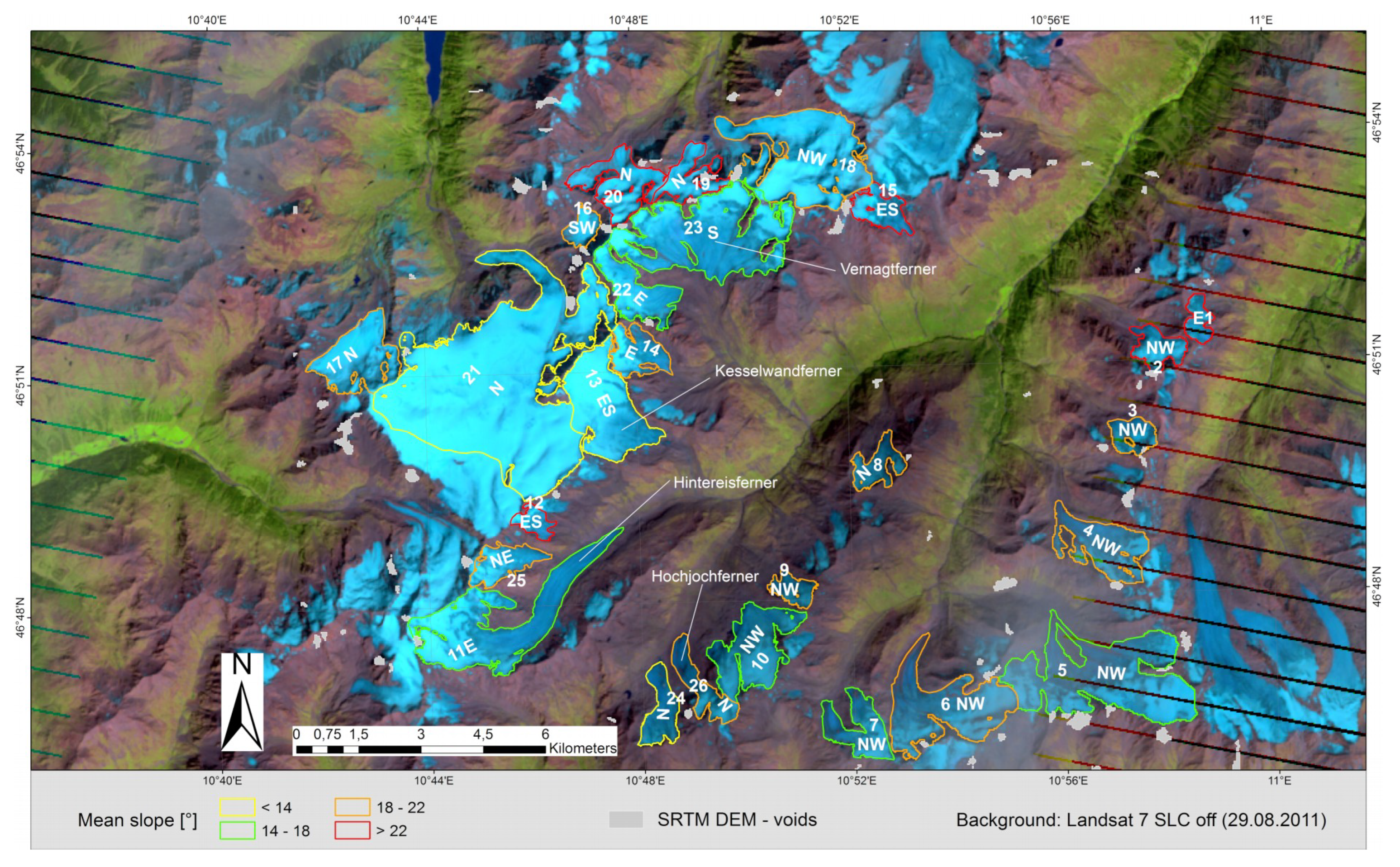
2. Study Region
3. Data and Data Preparation
3.1. Satellite Data
3.2. Digital Elevation Models
3.3. Glacier Outlines
3.4. Mass Balance Data
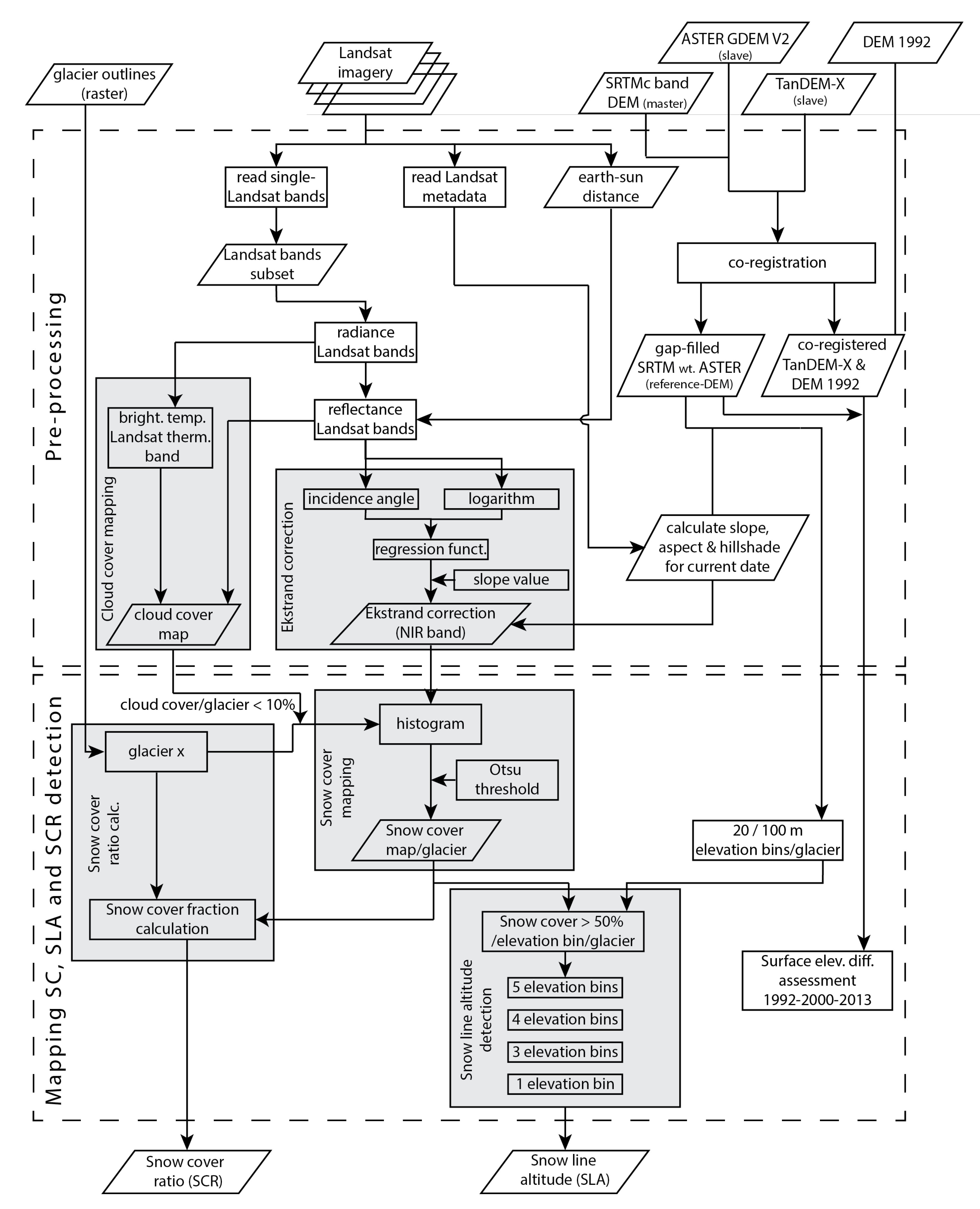
4. Methods (ASMAG Algorithm)
4.1. Data Pre-Processing
4.1.1. Import of Metadata and Landsat Image Sub-Setting
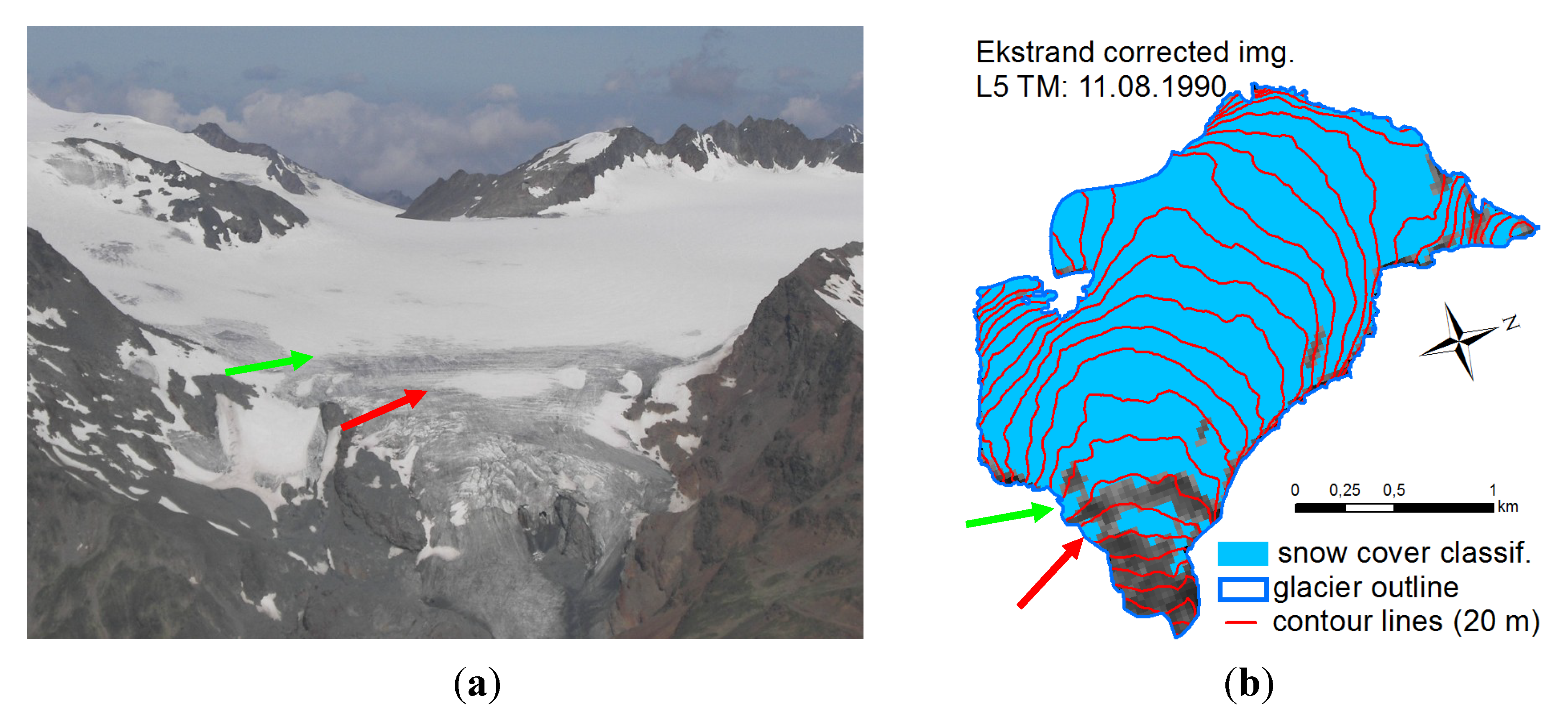
4.1.2. Topographic Normalization with the Ekstrand Correction
4.1.3. Cloud Cover Mapping
4.2. Snow Cover Mapping, Snow Line Altitude and Snow Cover Ratio Retrieval
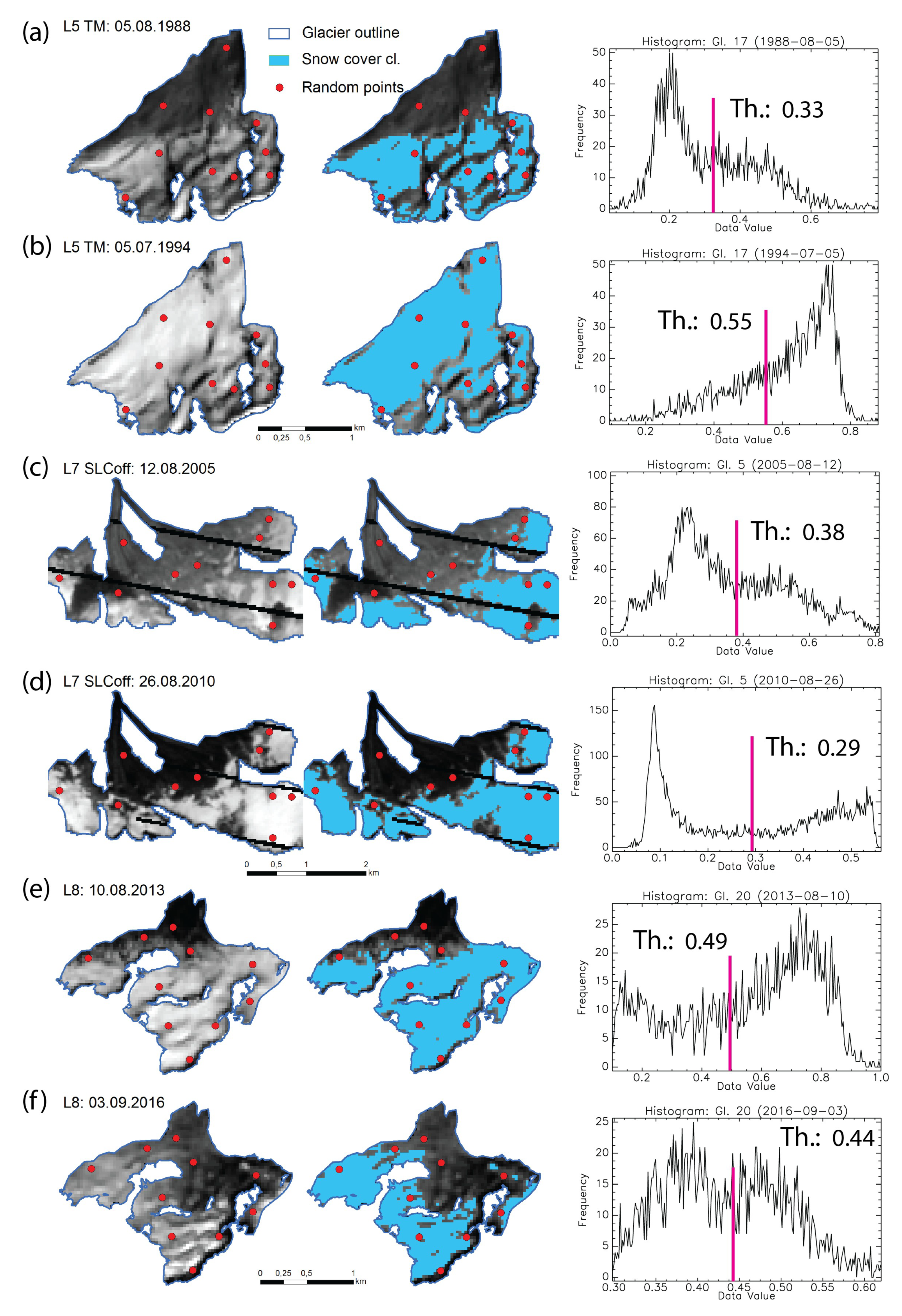
4.2.1. Snow Cover Mapping and the Snow Cover Ratio (SCR) for Individual Glaciers
4.2.2. Snow Line Altitude (SLA) Determination
4.3. Abramov Glacier (Kyrgyzstan) as an Independent Validation Region
4.4. Statistics
4.4.1. Snow Cover Mapping
4.4.2. Snow Line Altitude (SLA)
5. Results
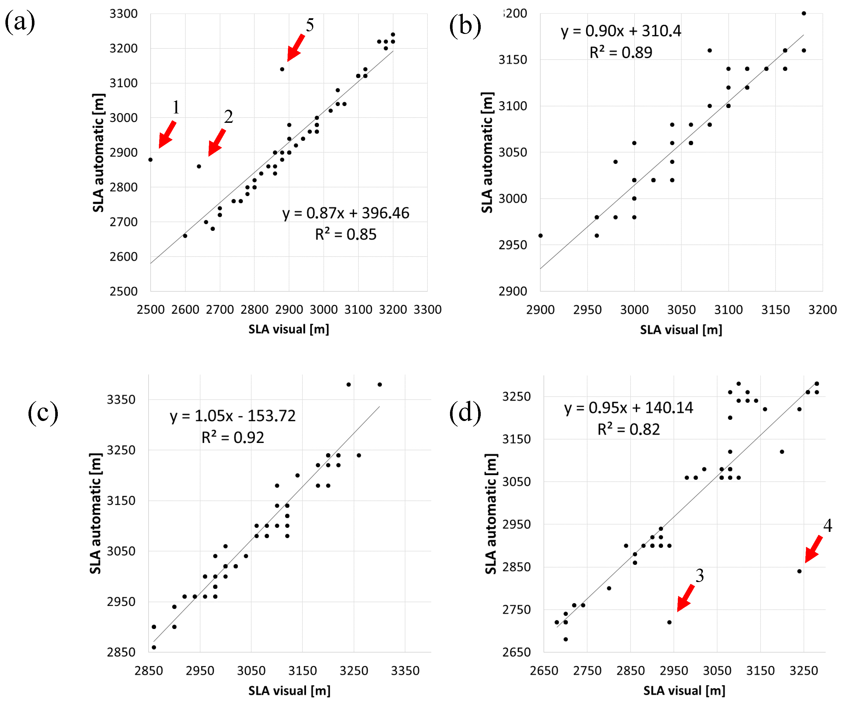
5.1. Performance of the Snow Cover Mapping and Snow Line Altitude Detection Method
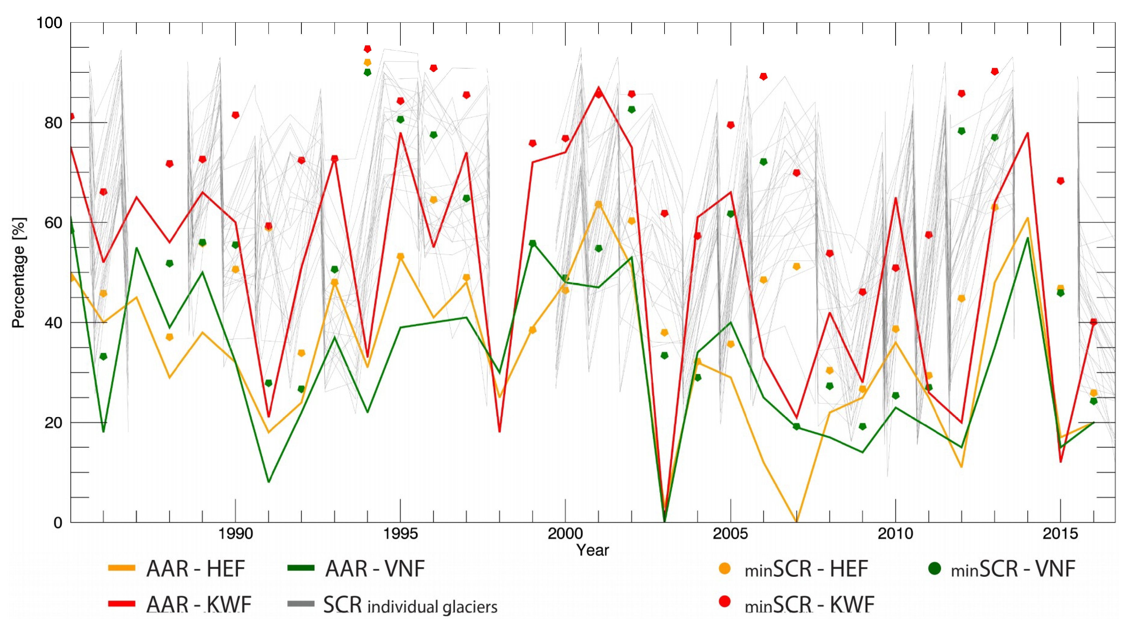
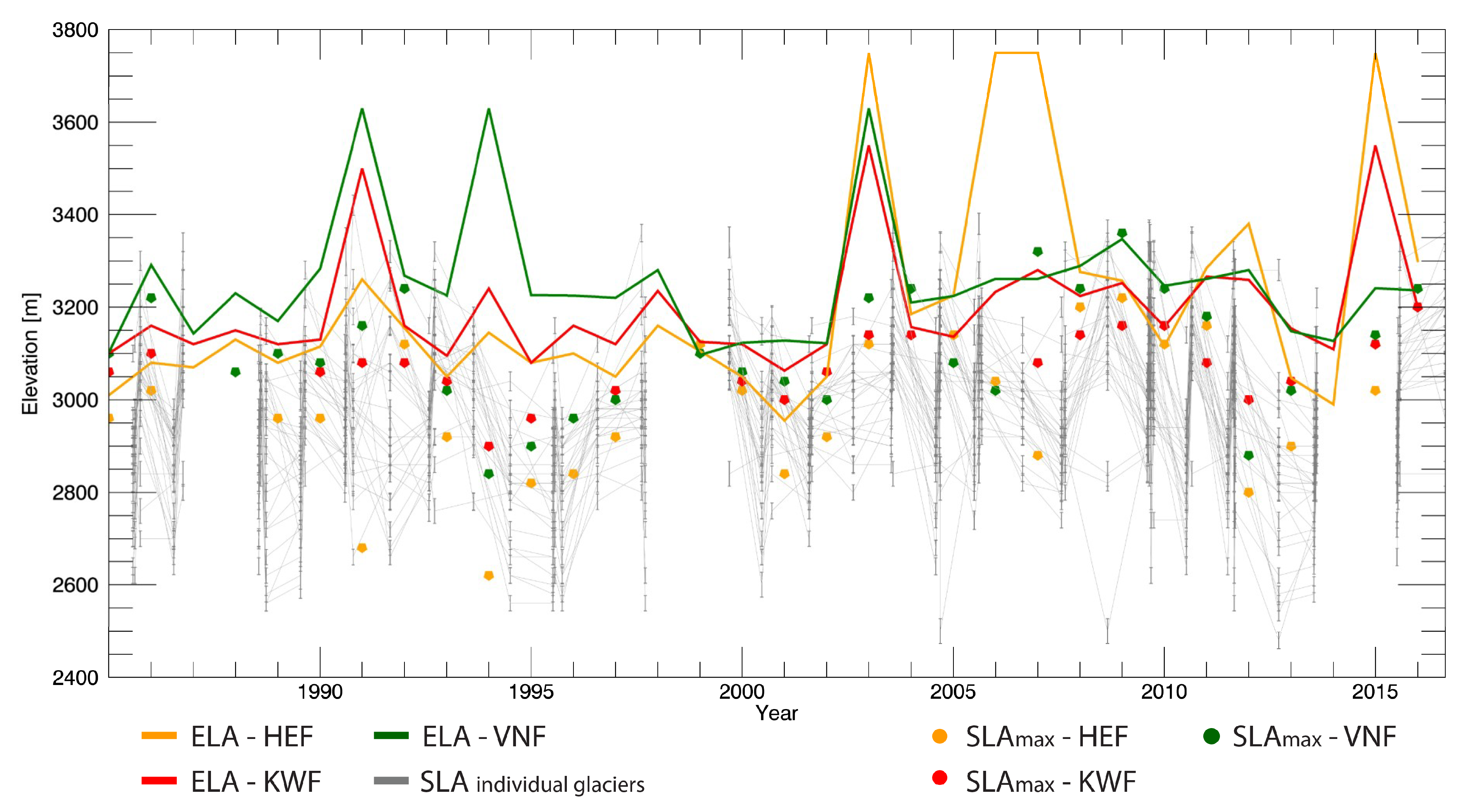
5.2. Snow Cover Ratio and Snow Line Altitude through Time
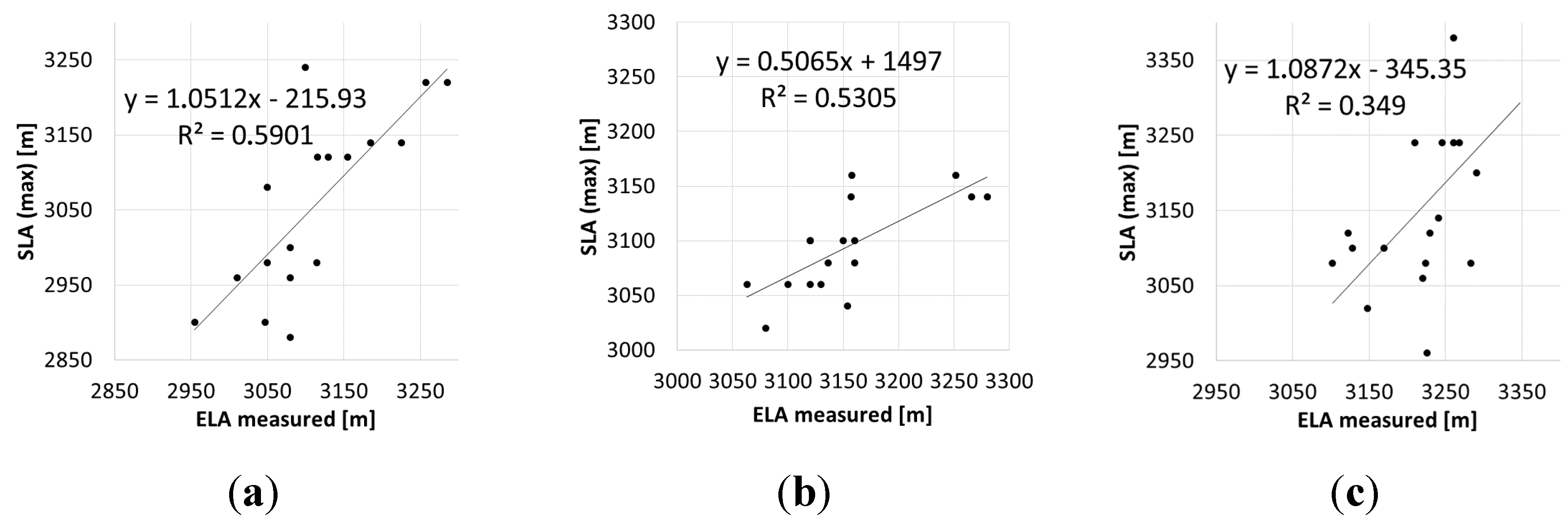
5.3. Maximum Snow Line Altitude Versus Equilibrium Line Altitude
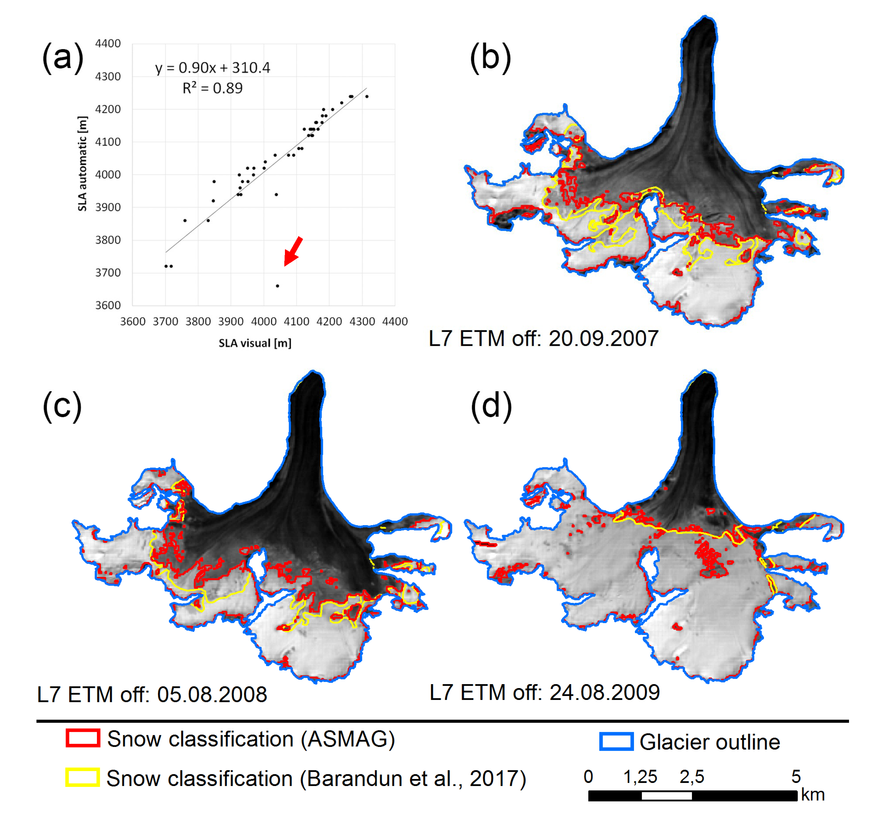
5.4. Abramov Glacier (Kyrgyzstan) SLA Results
6. Discussion
6.1. Results Obtained from ASMAG
6.1.1. Snow Cover Ratio SCR and AAR
6.1.2. Maximum SLA and ELA
6.1.3. Comparison to Other Studies
6.2. Data Constraints
6.2.1. Satellite Data
6.2.2. Digital Elevation Model
6.3. Methodological Constraints
7. Conclusions
Supplementary Materials
Author Contributions
Funding
Acknowledgments
Conflicts of Interest
Abbreviations
| AAR | Accumulation Area Ratio |
| ASMAG | Automated Snow Mapping on Glaciers |
| ASTER | Advanced Thermal Emission and Reflection Radiometer |
| DEM | Digital Elevation Model |
| DLR | Deutsches Forschungszentrum für Luft und Raumfahrt (German Aerospace Center) |
| DN | Digital Number |
| ELA | Equilibrium Line Altitude |
| ENVI | Environment for Visualizing Images (Geospatial Image Analysis Software) |
| ESA | European Space Agency |
| ETM+ | Enhanced Thematic Mapper + |
| GIS | Geographic Information System |
| HEF | Hintereisferner |
| HJF | Hochjochferner |
| IDL | Interactive Data Language |
| KWF | Kesselwandferner |
| L4/L5/L7/L8 | Landsat 4/5/7/8 |
| MODIS | Moderate-Resolution Imaging Spectroradiometer |
| MSI | Multispectral Instrument |
| MSS | MultiSpectral Scanner |
| NDSI | Normalised Difference Snow Index |
| NIR | Near Infrared |
| OLI | Operational Land Imager |
| SC | Snow Cover |
| SCA | Snow Cover Area |
| SCF | Snow Cover Fraction |
| SLA | Snow Line Altitude |
| SLC off | Scan Line Corrector; refers to all Landsat 7 images collected after May 31, 2003 |
| SPOT | Satellite Pour l’Observation de la Terre |
| SRTM | Shuttle Radar Topography Mission |
| STD | Standard Deviation |
| SWIR | Shortwave Infrared |
| TanDEM-X | Global TanDEM-X terrain model |
| TIRS | Thermal Infrared Sensor |
| TOAR | Top of Atmosphere Reflectance |
| TM | Thematic Mapper |
| USGS | United States Geological Survey |
| VNF | Vernagtferner |
References
- Kaser, G.; Grosshauser, M.; Marzeion, B. Contribution potential of glaciers to water availability in different climate regimes. Proc. Natl. Acad. Sci. USA 2010, 107, 20223–20227. [Google Scholar] [CrossRef] [PubMed]
- Huss, M.; Bookhagen, B.; Huggel, C.; Jacobsen, D.; Bradley, R.S.; Clague, J.J.; Vuille, M.; Buytaert, W.; Cayan, D.R.; Greenwood, G.; et al. Toward mountains without permanent snow and ice: Mountains without permanent snow and ice. Earth’s Future 2017, 5, 418–435. [Google Scholar] [CrossRef]
- Zemp, M.; Huss, M.; Thibert, E.; Eckert, N.; McNabb, R.; Huber, J.; Barandun, M.; Machguth, H.; Nussbaumer, S.U.; Gärtner-Roer, I.; et al. Global glacier mass changes and their contributions to sea-level rise from 1961 to 2016. Nature 2019, 568, 382–386. [Google Scholar] [CrossRef] [PubMed]
- Giesen, R.H.; Oerlemans, J. Climate-model induced differences in the 21st century global and regional glacier contributions to sea-level rise. Clim. Dyn. 2013, 7, 3283–3300. [Google Scholar] [CrossRef]
- Marzeion, B.; Champollion, N.; Haeberli, W.; Langley, K.; Leclercq, P.; Paul, F. Observation-based estimates of global glacier mass change and its contribution to sea-level change. Surv. Geophys. 2017, 38, 105–130. [Google Scholar] [CrossRef] [PubMed]
- Zemp, M.; Frey, H.; Gärtner-Roer, I.; Nussbaumer, S.U.; Hoelzle, M.; Paul, F.; Haeberli, W.; Denzinger, F.; Ahlstrøm, A.P.; Anderson, B.; et al. Historically unprecedented global glacier decline in the early 21st century. J. Glaciol. 2015, 61, 745–762. [Google Scholar] [CrossRef]
- Cogley, J.G. Geodetic and direct mass-balance measurements: Comparison and joint analysis. Ann. Glaciol. 2009, 50, 96–100. [Google Scholar] [CrossRef]
- Bolch, T. Climate change and glacier retreat in northern Tien Shan (Kazakhstan/Kyrgyzstan) using remote sensing data. Glob. Planet. Chang. 2007, 56, 1–12. [Google Scholar] [CrossRef]
- Rastner, P.; Joerg, P.C.; Huss, M.; Zemp, M. Historical analysis and visualization of the retreat of Findelengletscher, Switzerland, 1859–2010. Glob. Planet. Chang. 2016, 145, 67–77. [Google Scholar] [CrossRef]
- Peduzzi, P.; Herold, C.; Silverio, W. Assessing high altitude glacier thickness, volume and area changes using field, GIS and remote sensing techniques: The case of Nevado Coropuna (Peru). Cryosphere 2010, 4, 313–323. [Google Scholar] [CrossRef]
- Prinz, R.; Fischer, A.; Nicholson, L.; Kaser, G. Seventy-six years of mean mass balance rates derived from recent and re-evaluated ice volume measurements on tropical Lewis Glacier, Mount Kenya. Geophys. Res. Lett. 2011, 38. [Google Scholar] [CrossRef]
- Rabatel, A.; Bermejo, A.; Loarte, E.; Soruco, A.; Gomez, J.; Leonardini, G.; Vincent, C.; Sicart, J.E. Can the snowline be used as an indicator of the equilibrium line and mass balance for glaciers in the outer tropics? J. Glaciol. 2012, 58, 1027–1036. [Google Scholar] [CrossRef]
- Rabatel, A.; Dedieu, J.-P.; Vincent, C. Using remote-sensing data to determine equilibrium-line altitude and mass-balance time series: Validation on three French glaciers, 1994–2002. J. Glaciol. 2005, 51, 539–546. [Google Scholar] [CrossRef]
- Rabatel, A.; Letréguilly, A.; Dedieu, J.-P.; Eckert, N. Changes in glacier equilibrium-line altitude in the western Alps from 1984 to 2010: Evaluation by remote sensing and modeling of the morpho-topographic and climate controls. Cryosphere 2013, 7, 1455–1471. [Google Scholar] [CrossRef]
- Pelto, M. Utility of late summer transient snowline migration rate on Taku Glacier, Alaska. Cryosphere 2011, 5, 1127–1133. [Google Scholar] [CrossRef]
- Mathieu, R.; Chinn, T.; Fitzharris, B. Detecting the equilibrium-line altitudes of New Zealand glaciers using ASTER satellite images. N. Z. J. Geol. Geophys. 2009, 52, 209–222. [Google Scholar] [CrossRef]
- Cogley, J.G.; Hock, R.; Rasmussen, L.; Arendt, A.A.; Bauder, A.; Braithwaite, R.J.; Jansson, P.; Kaser, G.; Möller, M.; Nicholson, L. Glossary of glacier mass balance and related terms. IHP-VII Tech. Doc. Hydrol. 2011, 86, 1–124. [Google Scholar]
- Paul, F.; Escher-Vetter, H.; Machguth, H. Comparison of mass balances for Vernagtferner, Oetzal Alps, as obtained from direct measurements and distributed modeling. Ann. Glaciol. 2009, 50, 169–177. [Google Scholar] [CrossRef][Green Version]
- Hall, D.K.; Ormsby, J.P.; Bindschadler, R.A.; Siddalingaiah, H. Characterization of snow and ice reflectance zones on glaciers using Landsat Thematic Mapper data. Ann. Glaciol. 1987, 9, 104–108. [Google Scholar] [CrossRef]
- Paul, F.; Kääb, A. Perspectives on the production of a glacier inventory from multispectral satellite data in Arctic Canada: Cumberland Peninsula, Baffin Island. Ann. Glaciol. 2005, 42, 59–66. [Google Scholar] [CrossRef]
- Dozier, J. Spectral signature of alpine snow cover from the landsat thematic mapper. Remote Sens. Environ. 1989, 28, 9–22. [Google Scholar] [CrossRef]
- Østrem, G.; Haakensen, N.; Melander, O. Atlas over breer i Nord-Skandinavia. Glacier atlas of northern Scandinavia; Norges vassdrags- og elektrisitetsvesen: Oslo, Norway, 1973. [Google Scholar]
- Rott, H. Analyse der Schneeflächen auf Gletschern der Tiroler Zentralalpen aus Landsat-Bildern. Z. Gletsch. Glazialgeol. 1976, 12, 1–28. [Google Scholar]
- Shea, J.M.; Menounos, B.; Moore, R.D.; Tennant, C. An approach to derive regional snow lines and glacier mass change from MODIS imagery, western North America. Cryosphere 2013, 7, 667–680. [Google Scholar] [CrossRef]
- Brun, F.; Dumont, M.; Wagnon, P.; Berthier, E.; Azam, M.F.; Shea, J.M.; Sirguey, P.; Rabatel, A.; Ramanathan, A. Seasonal changes in surface albedo of Himalayan glaciers from MODIS data and links with the annual mass balance. Cryosphere 2015, 9, 341–355. [Google Scholar] [CrossRef]
- Williams, R.S.; Hall, D.; Benson, C.S. Analysis of glacier facies using satellite techniques. J. Glaciol. 1991, 37, 120–128. [Google Scholar] [CrossRef]
- Aniya, M.; Sato, H.; Naruse, R.; Skvarca, P.; Casassa, G. The use of satellite and airborne imagery to inventory outlet glaciers of the Southern Patagonia Icefield, South America. Photogramm. Eng. Remote Sens. 1996, 62, 1361–1369. [Google Scholar]
- Veettil, B.K.; Bremer, U.F.; de Souza, S.F.; Maier, É.L.B.; Simões, J.C. Variations in annual snowline and area of an ice-covered stratovolcano in the Cordillera Ampato, Peru, using remote sensing data (1986–2014). Geocarto Int. 2016, 31, 544–556. [Google Scholar] [CrossRef]
- Klein, A.G.; Isacks, B.L. Spectral mixture analysis of Landsat thematic mapper images applied to the detection of the transient snowline on tropical Andean glaciers. Glob. Planet. Chang. 1999, 22, 139–154. [Google Scholar] [CrossRef]
- Spiess, M.; Maussion, F.; Möller, M.; Scherer, D.; Schneider, C. Modis derived equilibrium line altitude estimates for purogangri ice cap, tibetan plateau, and their relation to climatic predictors (2001–2012). Geogr. Ann. Ser. APhysical Geogr. 2015, 97, 599–614. [Google Scholar] [CrossRef]
- Rabatel, A.; Dedieu, J.-P.; Thibert, E.; Letreguilly, A.; Vincent, C. 25 years (1981-2005) of equilibrium-line altitude and mass-balance reconstruction on Glacier Blanc, French Alps, using remote-sensing methods and meteorological data. J. Glaciol. 2008, 54, 307–314. [Google Scholar] [CrossRef]
- Barandun, M.; Huss, M.; Sold, L.; Farinotti, D.; Azisov, E.; Salzmann, N.; Usubaliev, R.; Merkushkin, A.; Hoelzle, M. Re-analysis of seasonal mass balance at Abramov glacier 1968–2014. J. Glaciol. 2015, 61, 1103–1117. [Google Scholar] [CrossRef]
- Mernild, S.H.; Pelto, M.; Malmros, J.K.; Yde, J.C.; Knudsen, N.T.; Hanna, E. Identification of snow ablation rate, ELA, AAR and net mass balance using transient snowline variations on two Arctic glaciers. J. Glaciol. 2013, 59, 649–659. [Google Scholar] [CrossRef]
- Klug, C.; Bollmann, E.; Galos, S.P.; Nicholson, L.; Prinz, R.; Rieg, L.; Sailer, R.; Stötter, J.; Kaser, G. A reanalysis of one decade of the mass balance series on Hintereisferner, Ötztal Alps, Austria: A detailed view into annual geodetic and glaciological observations. Cryosphere 2017, 1–38. [Google Scholar] [CrossRef]
- Kuhn, M. Fluctuations of climate and mass balance: Different responses of two adjacent glaciers. Z. Gletsch. Glazialgeol. 1985, 21, 409–416. [Google Scholar]
- Kuhn, M.; Dreiseitl, E.; Hofinger, S.; Markl, G.; Span, N.; Kaser, G. Measurements and models of the mass balance of Hintereisferner. Geogr. Annaler. Ser. A Physical Geogr. 1999, 81, 659–670. [Google Scholar] [CrossRef]
- Strasser, U.; Marke, T.; Braun, L.; Escher-Vetter, H.; Juen, I.; Kuhn, M.; Maussion, F.; Mayer, C.; Nicholson, L.; Niedertscheider, K.; et al. The Rofental: A high Alpine research basin (1890 m–3770 a.s.l.) in the Ötztal Alps (Austria) with over 150 years of hydro-meteorological and glaciological observations. Earth Syst. Sci. Data 2018, 10, 151–171. [Google Scholar] [CrossRef]
- Abermann, J.; Lambrecht, A.; Fischer, A.; Kuhn, M. Quantifying changes and trends in glacier area and volume in the Austrian Ötztal Alps (1969-1997-2006). Cryosphere 2009, 3, 205. [Google Scholar] [CrossRef]
- Rabatel, A.; Dedieu, J.P.; Vincent, C. Spatio-temporal changes in glacier-wide mass balance quantified by optical remote sensing on 30 glaciers in the French Alps for the period 1983–2014. J. Glaciol. 2016, 62, 1153–1166. [Google Scholar] [CrossRef]
- Bamler, R. The SRTM Mission: A world-wide 30 m resolution DEM from SAR interferometry in 11 days. In Proceedings of the Photogrammetric Week 99; Wichmann Verlag: Heidelberg, Germany; Stuttgart, Germany, 1999; pp. 145–154. [Google Scholar]
- Rodriguez, E.; Morris, C.S.; Belz, J.E. A global assessment of the SRTM performance. Photogramm. Eng. Remote Sens. 2006, 72, 249–260. [Google Scholar] [CrossRef]
- Fujisada, H.; Bailey, G.B.; Kelly, G.G.; Hara, S.; Abrams, M.J. ASTER DEM performance. IEEE Trans. Geosci. Remote Sens. 2005, 43, 2707–2714. [Google Scholar] [CrossRef]
- Rizzoli, P.; Martone, M.; Gonzalez, C.; Wecklich, C.; Borla Tridon, D.; Bräutigam, B.; Bachmann, M.; Schulze, D.; Fritz, T.; Huber, M.; et al. Generation and performance assessment of the global TanDEM-X digital elevation model. ISPRS J. Photogramm. Remote Sens. 2017, 132, 119–139. [Google Scholar] [CrossRef]
- Nuth, C.; Kääb, A. Co-registration and bias corrections of satellite elevation data sets for quantifying glacier thickness change. Cryosphere 2011, 5, 271–290. [Google Scholar] [CrossRef]
- Lambrecht, A.; Kuhn, M. Glacier changes in the Austrian Alps during the last three decades, derived from the new Austrian glacier inventory. Ann. Glaciol. 2007, 46, 177–184. [Google Scholar] [CrossRef]
- Chander, G.; Markham, B.L.; Helder, D.L. Summary of current radiometric calibration coefficients for Landsat MSS, TM, ETM+, and EO-1 ALI sensors. Remote Sens. Environ. 2009, 113, 893–903. [Google Scholar] [CrossRef]
- Landsat Project Science Office. Landsat 7 Science Data Users Handbook; Landsat Project Science Office: Greenbelt, MD, USA, 2006. [Google Scholar]
- Schmugge, T.; French, A.; Ritchie, J.C.; Rango, A.; Pelgrum, H. Temperature and emissivity separation from multispectral thermal infrared observations. Remote Sens. Environ. 2002, 79, 189–198. [Google Scholar] [CrossRef]
- Ekstrand, S. Landsat TM-based forest damage assessment: Correction for topographic effects. Photogramm. Eng. Remote Sens. 1996, 62, 151–162. [Google Scholar]
- Minnaert, M. The reciprocity principle in lunar photometry. Astrophys. J. 1941, 93, 403–410. [Google Scholar] [CrossRef]
- Teillet, P.M.; Guindon, B.; Goodenough, D.G. On the slope-aspect correction of multispectral scanner data. Can. J. Remote Sens. 1982, 8, 84–106. [Google Scholar] [CrossRef]
- Bippus, G. Characteristics of Summer Snow Areas on Glaciers Observed by Means of Landsat Data. Ph.D. Thesis, University of Innsbruck, Innsbruck, Austria, 2011. [Google Scholar]
- Irish, R.R. Landsat 7 automatic cloud cover assessment. In Proceedings of the AeroSense 2000; International Society for Optics and Photonics: Orlando, FL, USA, 2000; pp. 348–355. [Google Scholar]
- Yin, D.; Cao, X.; Chen, X.; Shao, Y.; Chen, J. Comparison of automatic thresholding methods for snow-cover mapping using Landsat TM imagery. Int. J. Remote Sens. 2013, 34, 6529–6538. [Google Scholar] [CrossRef]
- Otsu, N. A threshold selection method from gray-level histograms. IEEE Trans. Syst. Man. Cybern. 1979, 9, 62–66. [Google Scholar] [CrossRef]
- Härer, S.; Bernhardt, M.; Siebers, M.; Schulz, K. On the need for a time- and location-dependent estimation of the NDSI threshold value for reducing existing uncertainties in snow cover maps at different scales. Cryosphere 2018, 12, 1629–1642. [Google Scholar] [CrossRef]
- WMO, D.S. Seasonal Snow Cover. Available online: https://bit.ly/2XfsVpG (accessed on 13 June 2019).
- Fischer, A. Glaciers and climate change: Interpretation of 50 years of direct mass balance of Hintereisferner. Glob. Planet. Chang. 2010, 71, 13–26. [Google Scholar] [CrossRef]
- Barandun, M.; Huss, M.; Berthier, E.; Kääb, A.; Azisov, E.; Bolch, T.; Usubaliev, R.; Hoelzle, M. Multi-decadal mass balance series of three Kyrgyz glaciers inferred from transient snowline observations. Cryosphere 2017, 1–31. [Google Scholar] [CrossRef]
- Abermann, J. Glaciers in Austria; Past and Present: Innsbruck, Austria, 2011. [Google Scholar]
- Hantel, M.; Hirtl-Wielke, L.-M. Sensitivity of Alpine snow cover to European temperature. Int. J. Climatol. 2007, 27, 1265–1275. [Google Scholar] [CrossRef]
- Klein, G.; Vitasse, Y.; Rixen, C.; Marty, C.; Rebetez, M. Shorter snow cover duration since 1970 in the Swiss Alps due to earlier snowmelt more than to later snow onset. Clim. Chang. 2016, 139, 637–649. [Google Scholar] [CrossRef]
- Dumont, M.; Gardelle, J.; Sirguey, P.; Guillot, A.; Six, D.; Rabatel, A.; Arnaud, Y. Linking glacier annual mass balance and glacier albedo retrieved from MODIS data. Cryosphere 2012, 6, 1527–1539. [Google Scholar] [CrossRef]
- Greuell, W.; Kohler, J.; Obleitner, F.; Glowacki, P.; Melvold, K.; Bernsen, E.; Oerlemans, J. Assessment of interannual variations in the surface mass balance of 18 Svalbard glaciers from the Moderate Resolution Imaging Spectroradiometer/Terra albedo product. J. Geophys. Res. 2007, 112. [Google Scholar] [CrossRef]
- Sirguey, P.; Still, H.; Cullen, N.J.; Dumont, M.; Arnaud, Y.; Conway, J.P. Reconstructing the mass balance of Brewster Glacier, New Zealand, using MODIS-derived glacier-wide albedo. Cryosphere 2016, 10, 2465. [Google Scholar] [CrossRef]
- Paul, F.; Winsvold, S.; Kääb, A.; Nagler, T.; Schwaizer, G. Glacier remote sensing using Sentinel-2. Part II: Mapping glacier extents and surface facies, and comparison to Landsat 8. Remote Sens. 2016, 8, 575. [Google Scholar] [CrossRef]
- Gardelle, J.; Berthier, E.; Arnaud, Y. Slight mass gain of Karakoram glaciers in the early twenty-first century. Nat. Geosci. 2012, 5, 322–325. [Google Scholar] [CrossRef]
- Rignot, E.; Echelmeyer, K.; Krabill, W. Penetration depth of interferometric synthetic-aperture radar signals in snow and ice. Geophys. Res. Lett. 2001, 28, 3501–3504. [Google Scholar] [CrossRef]
- Mukherjee, S.; Joshi, P.K.; Mukherjee, S.; Ghosh, A.; Garg, R.D.; Mukhopadhyay, A. Evaluation of vertical accuracy of open source Digital Elevation Model (DEM). Int. J. Appl. Earth Obs. Geoinf. 2013, 21, 205–217. [Google Scholar] [CrossRef]
- Kääb, A.; Berthier, E.; Nuth, C.; Gardelle, J.; Arnaud, Y. Contrasting patterns of early twenty-first-century glacier mass change in the Himalayas. Nature 2012, 488, 495–498. [Google Scholar] [CrossRef] [PubMed]
- Scherler, D.; Wulf, H.; Gorelick, N. Global Assessment of Supraglacial Debris-Cover Extents. Geophys. Res. Lett. 2018, 45, 798–805. [Google Scholar] [CrossRef]


| Year | Scene Count | Year | Scene Count | Year | Scene Count | Year | Scene Count | Year | Scene Count | Year | Scene Count |
|---|---|---|---|---|---|---|---|---|---|---|---|
| 1985 | 3 | 1991 | 1 | 1996 | 1 | 2002 | 1 | 2007 | 2 | 2012 | 1 |
| 1986 | 2 | 1992 | 2 | 1997 | 2 | 2003 | 2 | 2008 | 1 | 2013 | 3 |
| 1988 | 3 | 1993 | 1 | 1999 | 1 | 2004 | 3 | 2009 | 6 | 2015 | 3 |
| 1989 | 2 | 1994 | 1 | 2000 | 2 | 2005 | 3 | 2010 | 2 | 2016 | 2 |
| 1990 | 3 | 1995 | 3 | 2001 | 2 | 2006 | 1 | 2011 | 4 | Total: | 63 |
| Spacecraft | Sensor/Operation Time | Image Bands | Spatial Resolution Optical/Thermal [m] | Radiometric Resolution [bit] | Scene Count |
|---|---|---|---|---|---|
| Landsat 4 | TM (1982–1993) | 7 | 30/120 | 8 | 2 |
| Landsat 5 | MSS (1984–2013) | 4 | 60/none | 8 | 1 |
| Landsat 5 | TM (1984–2013) | 7 | 30/120 | 8 | 39 |
| Landsat 7 | ETM SLC on (1999–2003) | 9 | 30/60 | 8 | 4 |
| Landsat 7 | ETM SLC off (2003–2016) | 9 | 30/60 | 8 | 13 |
| Landsat 8 | OLI TIRS (2013–2016) | 11 | 30/100 | 12 | 4 |
| Coreg. Parameters | TanDEM-X [m] | ASTER GDEM V2 [m] |
|---|---|---|
| before | −57.8 | 10.8 |
| STD before | 10.4 | 13.07 |
| ΔX | −31.7 | −32.5 |
| ΔY | −11 | −8 |
| ΔZ | −54.5 | −7.5 |
| after | 0.02 | −0.06 |
| STD after | 6.47 | 10.22 |
| Sensor | Date | Points (A/V) | Percent | Sensor | Date | Points (A/V) | Percent |
|---|---|---|---|---|---|---|---|
| ETM SLC on | 13.09.1999 | 5/6 | 83 | OLI | 10.08.2013 | 6/8 | 75 |
| ETM SLC on | 20.08.2002 | 4/6 | 67 | OLI | 03.09.2016 | 3/3 | 100 |
| ETM SLC off | 12.08.2005 | 3/3 | 100 | TM | 05.08.1988 | 6/6 | 100 |
| ETM SLC off | 26.08.2010 | 7/7 | 100 | TM | 05.07.1994 | 9/9 | 100 |
| 2500–2600 (m) | 2600–2700 (m) | 2700–2800 (m) | 2800–2900 (m) | |
|---|---|---|---|---|
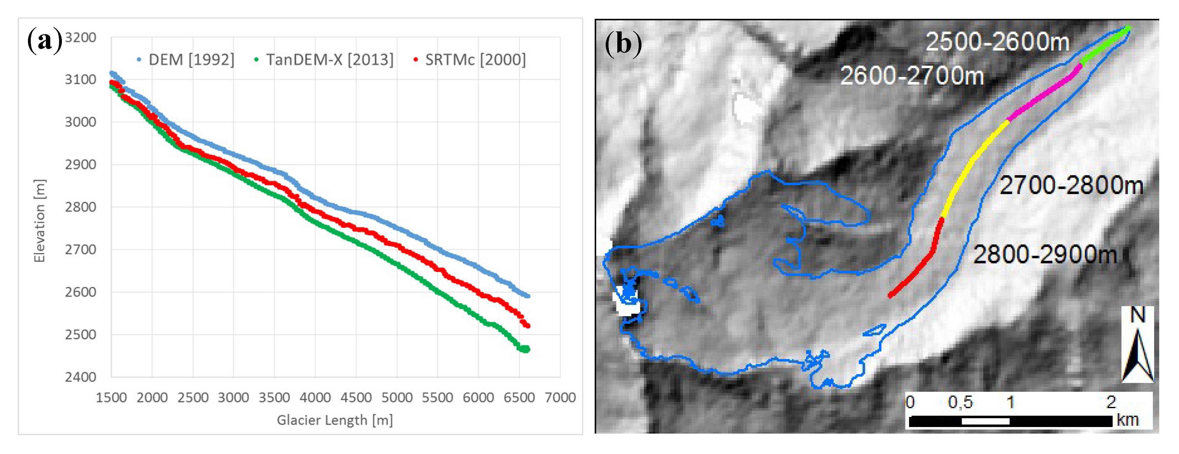
| 1992–2000 [m] | 64 | 54 | 40 | 32 |
| 2013–2000 [m] | −60 | −48 | −32 | −21 |
© 2019 by the authors. Licensee MDPI, Basel, Switzerland. This article is an open access article distributed under the terms and conditions of the Creative Commons Attribution (CC BY) license (http://creativecommons.org/licenses/by/4.0/).
Share and Cite
Rastner, P.; Prinz, R.; Notarnicola, C.; Nicholson, L.; Sailer, R.; Schwaizer, G.; Paul, F. On the Automated Mapping of Snow Cover on Glaciers and Calculation of Snow Line Altitudes from Multi-Temporal Landsat Data. Remote Sens. 2019, 11, 1410. https://doi.org/10.3390/rs11121410
Rastner P, Prinz R, Notarnicola C, Nicholson L, Sailer R, Schwaizer G, Paul F. On the Automated Mapping of Snow Cover on Glaciers and Calculation of Snow Line Altitudes from Multi-Temporal Landsat Data. Remote Sensing. 2019; 11(12):1410. https://doi.org/10.3390/rs11121410
Chicago/Turabian StyleRastner, Philipp, Rainer Prinz, Claudia Notarnicola, Lindsey Nicholson, Rudolf Sailer, Gabriele Schwaizer, and Frank Paul. 2019. "On the Automated Mapping of Snow Cover on Glaciers and Calculation of Snow Line Altitudes from Multi-Temporal Landsat Data" Remote Sensing 11, no. 12: 1410. https://doi.org/10.3390/rs11121410
APA StyleRastner, P., Prinz, R., Notarnicola, C., Nicholson, L., Sailer, R., Schwaizer, G., & Paul, F. (2019). On the Automated Mapping of Snow Cover on Glaciers and Calculation of Snow Line Altitudes from Multi-Temporal Landsat Data. Remote Sensing, 11(12), 1410. https://doi.org/10.3390/rs11121410