Performance Impact of Parameter Tuning on the CCSDS-123.0-B-2 Low-Complexity Lossless and Near-Lossless Multispectral and Hyperspectral Image Compression Standard ^†

Abstract

This article studies the performance impact related to different parameter choices for the new CCSDS-123.0-B-2 Low-Complexity Lossless and Near-Lossless Multispectral and Hyperspectral Image Compression standard. This standard supersedes CCSDS-123.0-B-1 and extends it by incorporating a new near-lossless compression capability, as well as other new features. This article studies the coding performance impact of different choices for the principal parameters of the new extensions, in addition to reviewing related parameter choices for existing features. Experimental results include data from 16 different instruments with varying detector types, image dimensions, number of spectral bands, bit depth, level of noise, level of calibration, and other image characteristics. Guidelines are provided on how to adjust the parameters in relation to their coding performance impact.

1. Introduction

It is well known that space-borne remote-sensing instruments are often the source of large volumes of data and that, due to constraints on the down-link channel, these data need to be compressed [1,2,3]. In this regard, the Consultative Committee for Space Data Systems (CCSDS) has standardized several data-compression techniques [4,5,6].

Very recently, the CCSDS has superseded Issue 1 of the Lossless Multispectral & Hyperspectral Image Compression standard [7] with Issue 2 titled Low-Complexity Lossless and Near-Lossless Multispectral and Hyperspectral Image Compression (CCSDS-123.0-B-2) [8]. The original issue of the standard employed the fast lossless compression algorithm [9,10] to achieve state-of-the-art compression performance, whilst being implemented in resource-constrained hardware available for space operation [11,12,13,14,15,16,17,18,19].

The new Issue 2 extends the previous issue, primarily by incorporating support for near-lossless compression, while retaining lossless compression capabilities (and all other features) of Issue 1.

The cornerstone behind Issue 2 of the standard is the newly-available option for near-lossless compression provided by an in-loop quantizer embedded in the prediction stage of the compressor. In addition, Issue 2 incorporates several other features including: prediction representatives, weight exponent offsets, narrow prediction modes, and a new hybrid entropy coder. The authors assume that readers are familiar with its contents (an overview of the new standard is provided in [20]).

As with the previous Issue 1, several tunable parameters are available to implementers and end-users. Employing different settings for these parameters may allow an implementer to achieve different trade-offs between implementation complexity and compression efficiency or may allow an end-user to fine-tune compression performance for particular datasets. This paper studies these parameters and provides some guidelines on how to adjust them to achieve high coding efficiency based on a representative corpus of multi- and hyper-spectral images.

The current study includes revisiting our previous assessment of parameter settings under lossless compression [21,22] while considering the newly-available coding options, in addition to providing new guidelines for both old and new coding options for near-lossless compression.

This paper is organized as follows. Section 2 describes the experimental methodology. Section 3 reports the principal experimental results and provides usage guidelines. Finally, some conclusions close this document.

2. Experimental Approach and Default Settings

The new CCSDS-123.0-B-2 provides more than twenty configuration parameters, with most of these parameters having a direct impact on the compression performance of an implementation. Moreover, the performance impact of one parameter may depend on the values set for all the remaining ones. Given these interactions and the large number of parameters, any exhaustive exploration of the configuration space will rapidly hit a complexity wall. Hence, any reasonable experimental study requires a pragmatic approach to the exploration of the configuration space.

It is expected that different encoding configurations yield not only different coding performances, i.e., smaller compressed files, but also different implementation considerations, such as FPGA area utilization, required memory buffers, etc. However, these are strongly dependent on the implementation strategy and technology employed. This paper does not try to address these implementation considerations and focuses exclusively on coding performance, which does not depend on the implementation approach.

The approach followed in the parameter study presented in this paper is as follows. First, an initial configuration for a CCSDS-123.0-B-2 encoder has been drawn from the authors’ prior experiences and previous parameter assessments [22] (Annex C). Then, the effects of each of the parameters have been studied (one or a few at a time), and the configuration has been adjusted based on the outcomes of those analyses. Several iterations have been performed until a reasonable final configuration reached a local performance maximum.

This article reports the studies for parameters with the most significant performance impacts, where one or more parameters are studied independently, while the rest are set to default values, as reported in

Table 1. Default predictor settings employed in the experimental results, unless otherwise indicated.

Parameter Name	Symbol	Default Value	Description
Sample Encoding Order		Band interleaved by pixel (BIP)	The order in which mapped quantizer indexes are encoded by the entropy coder
Entropy Coder Type		Hybrid	Indicates which entropy coding option is employed
Quantizer Fidelity Control Method		Absolute error limits or lossless	Enables or disables absolute and relative error limits
Number of Prediction Bands	P	3	Number of previous bands used to perform prediction
Register Size	R	64	Size of the register used in prediction calculation
Local Sum Type		(Image dependent)	Identifies neighborhood used to calculate local sums
Prediction Mode		(Image dependent)	Indicates whether directional local differences are used in the prediction calculation
Weight Component Resolution	$\mathsf{\Omega }$	19	Determines the number of bits used to represent each weight vector component
Weight Initialization Method		Default	Determines initial values of weight vector components
Weight Initialization Table	$\left\{{\mathsf{\Lambda }}_z\right\}$	(Unused)	Defines the initial weight components under custom weight initialization
Weight Initialization Resolution	Q	(Unused)	Determines the precision of the initial weight components under custom initialization
Weight Update Scaling Exponent Initial Parameter	${\nu }_{\min }$	-1	Determines initial rate at which the predictor adapts the weight vector to input
Weight Update Scaling Exponent Final Parameter	${\nu }_{\max }$	$7-{\varphi }_z$	Determines the final rate at which the predictor adapts the weight vector to input
Weight Update Scaling Exponent Change Interval	$t_{\mathrm{inc}}$	26	Determines the interval between increments to the weight update scaling exponent
Weight Update Scaling Exponent Offsets	$\{{\zeta }_z^{\left(i\right)}\}$, $\left\{{\zeta }_z^{*}\right\}$	All are set to 0	Offsets the exponent of each predictor weight update calculation
Periodic Error Limit Updating		Disabled	Enables or disables periodic updates of error limits
Sample Representative Resolution	$\mathsf{\Theta }$	3	Determines the precision of sample representative calculations
Sample Representative Offset 1	$\left\{{\psi }_z\right\}$	7	Controls the offset from the center of the quantizer bin in the sample representative calculation.
Band Varying Offset		Disabled (all ${\psi }_z$ are equal)	Enables the use of different values for each element in $\left\{{\psi }_z\right\}$
Sample Representative Damping	$\left\{{\varphi }_z\right\}$	(Image dependent)	Controls the tradeoff between the predicted sample value and offset bin center in the sample representative calculation
Band Varying Damping		Disabled (all ${\varphi }_z$ are equal)	Enables the use of different values for each element in $\left\{{\varphi }_z\right\}$

${}^1$ When the quantizer fidelity control method is set to lossless, the sample representative offset parameter does not influence compression performance. However, its actual value is set to 0, as mandated in the standard.

and

Table 2. Default entropy encoder settings employed in the experimental results, unless otherwise indicated.

Parameter Name	Symbol	Default Value	Description
Unary Length Limit	$U_{\max }$	18	Limits the maximum length of any encoded sample
Rescaling Counter Size	${\gamma }^{*}$	6	Determines the interval between rescaling of the counter and accumulator
Initial Count Exponent	${\gamma }_0$	1	Sets the initial counter value
Initial High-resolution Accumulator Value	$\{{\tilde{\mathsf{\Sigma }}}_z\left(0\right)\}$	0	Sets an initial accumulator value for each band

. Defaults are based on the final configuration described in the previous paragraph.

In order to obtain relevant experimental results, a curated corpus of images is employed, encompassing images acquired by 16 different instruments, of varying processing levels, bit depths, and dimensions. The corpus is a superset of the publicly-available corpus used in the course of developing the CCSDS-123.0-B-1 recommendation [23].

Table 3. Summary of the corpus images and their properties.

Instrument	Image Type	Bit Depth	Number of Bands	Width	Height
AIRS	raw	14	1501	90	135 × 10
AVIRIS	raw	12	224	{614, 680}	512
AVIRIS	calibrated	16	224	677	512 × 5
AVIRIS	raw	16	224	680	512 × 5
AVIRIS-NG	radiance	14	432	598	512 × 4
AVIRIS-NG	raw	14	432	640	512 × 4
CASI	raw	12	72	405	2852
CASI	raw	12	72	406	1225
CRISM	FRT, raw	12	545	640	{420 × 4, 450, 480 × 2, 510 × 2}
CRISM	HRL, raw	12	545	320	{420, 450 × 2, 480}
CRISM	MSP, raw	12	74	64	2700 × 7
HICO	calibrated	14	128	512	2000 × 2
Hyperion	raw	12	242	256	{1024, 3176, 3187, 3242}
IASI	calibrated	12	8461	66	60 × 4
Landsat	raw	8	6	1024	1024 × 3
M3	global, radiance	12	85	304	512 × 4
M3	global, raw	12	86	320	512 × 2
M3	target, raw	12	260	640	512 × 3
MODIS	night, raw	12	17	2030	1354 × 5
MODIS	day, raw	12	14	2030	1354 × 5
MODIS	500 m, raw	12	5	4060	2708 × 5
MODIS	250 m, raw	12	2	8120	5416 × 5
MSG	calibrated	10	11	3712	3712 × 3
Pleiades	HR, simulated	12	4	224	{2456, 3928}
Pleiades	misregistered, sim.	12	4	296	2448 × 4
SFSI	raw	12	240	496	140 × 1
SPOT-5	HRG, processed	8	3	1024	1024 × 3
Vegetation	raw	10	4	1728	{10,080 × 2, 10,193 × 2}

summarizes the corpus images and their properties. The number of images available for the each instrument is indicated through the use of × and $\{·\}$ in the width and height columns of the table.

The default values for three of the parameters presented in Table 1 are adjusted to account for the specific characteristics of each instrument whenever experimental data presented in Section 3 suggest that the same parameter value is not adequate for all instruments. These adjustments are as follows. For the local sum type parameter, a value of wide column-oriented is employed for the CRISM, Hyperion, M3, and MODIS day and night images, while a value of wide neighbor-oriented is employed otherwise. A full prediction mode is employed for all images, except for the AIRS, AVIRIS 12-bit, CASI, CRISM, Hyperion, IASI, M3, and MODIS day and night images. The value of the sample representative damping parameter is set to five for the AVIRIS NG, HICO, and SFSI images; to three for the AIRS, AVIRIS 12-bit raw, CASI, CRISM, Hyperion, and M3 target images; and to zero for the rest of the images.

3. Experimental Results

This section analyzes how the principal parameters for the new Issue 2 affect compression performance. The experimental results are organized into four subsections, each focusing on one of the key new features introduced in Issue 2, examining both lossless and near-lossless compression.

While experiments have been performed for a large number of images, due to space constraints, this document only reports results covering the most significant behaviors for some of the experiments. In addition, averaged results are reported when multiple images are available for an instrument type for the same reason (averages are weighted by image size).

Other experimental restrictions, intended to obtain a reasonably-sized set of results, are as follows. When compression is not lossless, reconstructed image fidelity is controlled using band-independent absolute error limits via the value of the integer absolute error limit constant parameter $A^{*}$. Note that setting $A^{*}=0$ yields lossless compression and is equivalent to selecting the fidelity control method to be lossless, apart from some minor differences in the compressed image header. Relative error limits are not used, and periodic error limit updating is not used, i.e., a fixed value of $A^{*}$ is used for the entire image (see [24,25] for alternative error limit adjustment strategies). Per-band parameter adjustment and custom weight initialization are purposely left out of the article as well. In addition, the studies related to the following less relevant parameters are omitted for conciseness: weight component resolution, register size, sample-adaptive and block-adaptive encoder initialization.

Even with all the aforementioned constraints, the experimental results presented in this section are the outcome of more than two million individual compression experiments where an image is compressed with an implementation fully compliant with CCSDS-123.0-B-2. In terms of the volume of data processed, more than 100 TB of image data have been compressed to produce these results.

3.1. Local Sum Type, Prediction Mode, and Number of Prediction Bands

The choices of local sum type, prediction mode, and number of prediction bands (P) determine the prediction neighborhood, i.e., the neighboring samples that directly influence the prediction of a given image sample.

Different choices for these three parameters strongly influence the implementation complexity due to the varying data dependencies of each mode. In particular, to facilitate pipelining in a hardware implementation, Issue 2 introduces a new option to use narrow local sums as an alternative to the existing local sums, which are now called wide. However, note that the use of narrow local sums and full prediction mode might be an unlikely combination in practice since full prediction mode has data dependencies that may quash any advantage provided by narrow local sums over their wide counterparts.

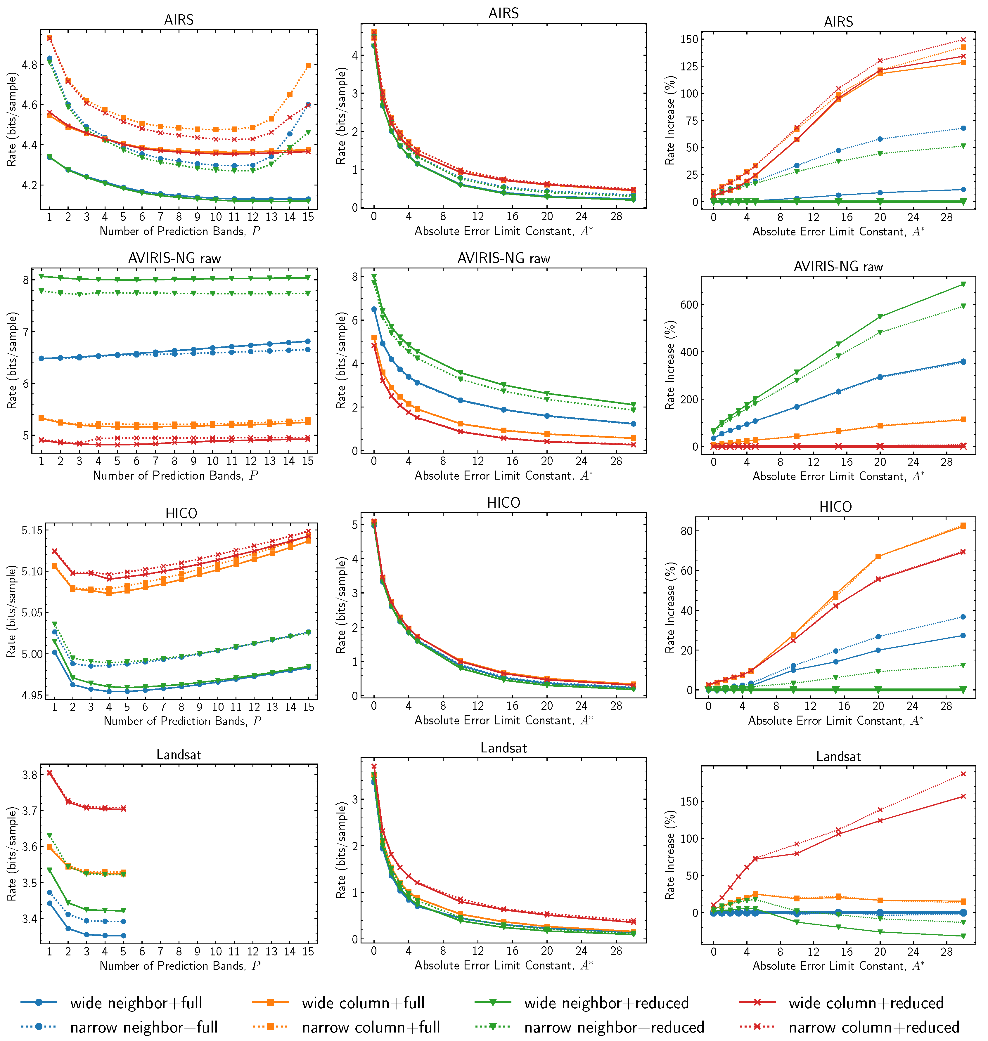
Figure 1 reports results for all choices of the local sum type and prediction mode under a varying number of prediction bands and an absolute error limit. As in Issue 1, the choice of both local sum type and prediction mode can have a huge impact on compression performance, and the optimum choices strongly depend on the image type. However, results suggest that the best choices remain constant regardless of the number of prediction bands employed and that the same recommendations available for Issue 1 [22] are applicable to Issue 2 when in lossless mode; i.e., the use of column-oriented local sums and reduced mode is still recommended for images that exhibit significant streaking artifacts parallel to the y direction (e.g., AVIRIS-NG raw images), whereas for images without such artifacts, neighbor-oriented local sums provide the best performance.

Varying the absolute error limit constant appears to generally have little impact on which choice of local sum type and prediction mode is optimum. Results may vary at very high (in relation to image bit depth) quantization levels, as indicated for the Landsat images.

The use of narrow local sums nearly always results in some performance penalty. The exception here is the use of neighbor-oriented local sums on AVIRIS-NG images. However, in this case, the lower complexity column-oriented local sums perform substantially better anyway. Narrow and wide column-oriented local sums differ only for the first image frame (i.e., at $y=0$), and thus tend to yield only a small performance difference as long as image height is not small. For neighbor-oriented local sums, the penalty for using narrow instead of wide sums becomes significant (10 percent or more in several cases) at larger values of absolute error.

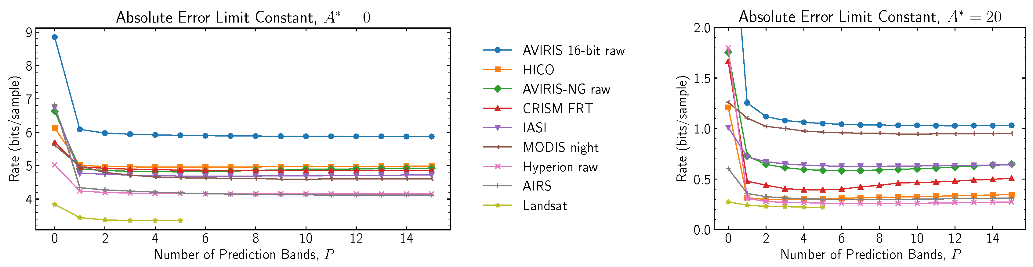
Regarding the selection of the number of prediction bands, as shown in Figure 1 and Figure 2, using a very large value of P provides no appreciable improvement for most images. In addition, a large P value may even slightly decrease the performance for some images, which could be explained by the slower adaptation caused by a larger weight vector. A default value of $P=3$ appears reasonable for both lossless and near-lossless compression.

3.2. Adaptation Rate and Sample Representatives

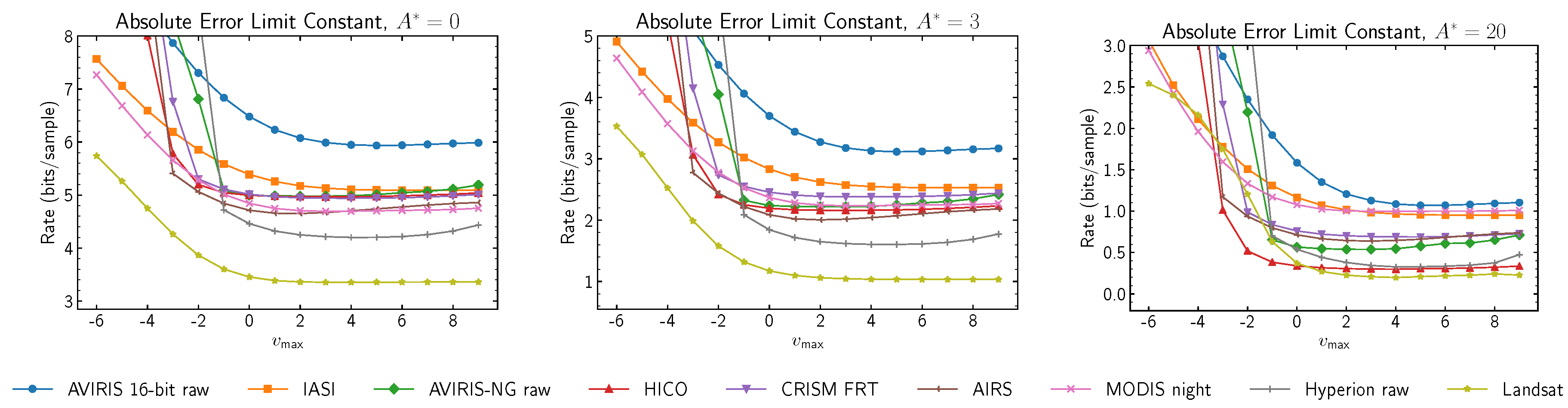
The rate at which the predictor adapts to varying image characteristics is controlled by ${\nu }_{\min }$ and $t_{\mathrm{inc}}$ initially and by ${\nu }_{\max }$ once a steady state is reached. Figure 3 shows the performance of different steady-state learning rates, ${\nu }_{\max }$, under varying quantization levels. The results indicate that adequate values for ${\nu }_{\max }$ are generally invariant to the quantization level, though a more pronounced decrease in performance as ${\nu }_{\max }$ becomes smaller is evident.

Figure 4 reports on the performance impact of extreme choices for ${\nu }_{\min }$ and $t_{\mathrm{inc}}$. In images with few samples per band, parameters affecting the initial learning rate control predictor learning rate for most (or all) samples in each band, thus, have a significant impact on overall prediction performance. This effect diminishes as images grow in spatial size.

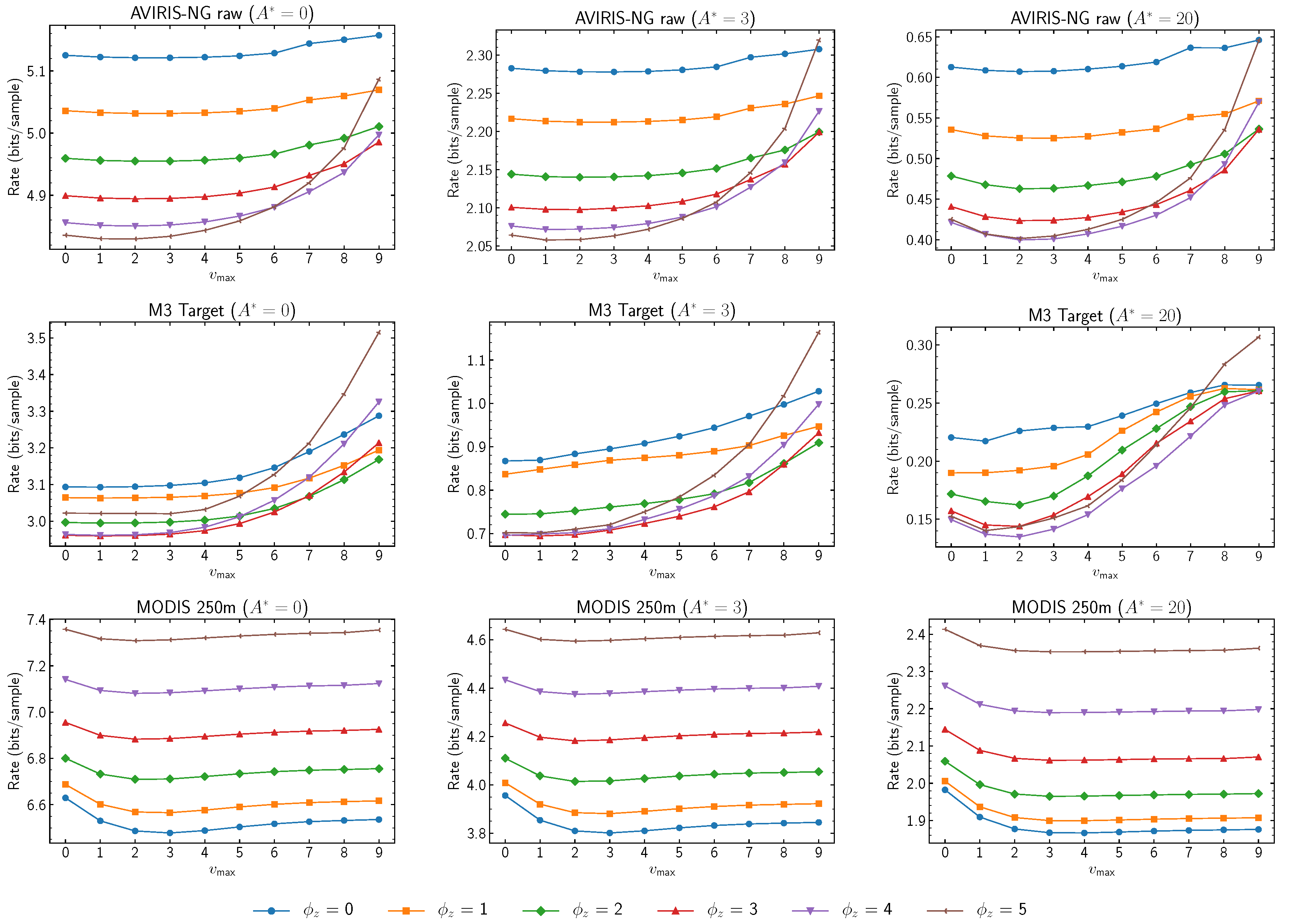
The newly-introduced sample representatives and the associated damping parameter ${\varphi }_z$ interact significantly with the predictor learning rate. The damping parameter interacts with the predictor feedback loop in a manner that may prevent image noise from influencing the training process, and thus improve coding performance for noisy images. Figure 5 shows coding performances obtained for varying damping values in relation to ${\nu }_{\max }$. Substantial benefits may be obtained by properly-selected damping values. In our experiments, using sample representative resolution $\mathsf{\Theta }=3$, the best results have been obtained by employing a strong damping value of five for AVIRIS-NG, HICO, and SFSI; by employing a medium value of three for AIRS, AVIRIS 12-bit raw, CASI, CRISM, Hyperion, and M3 target; and no damping (${\varphi }_z=0$) for the remaining instruments. Visual inspection of image noise levels seem to corroborate that noise levels are a determining factor in the selection of the damping value. However, these results do not exclude the possibility that other factors might also be relevant to the selection of damping values, such as instrument resolution or other forms of signal distortion different than noise.

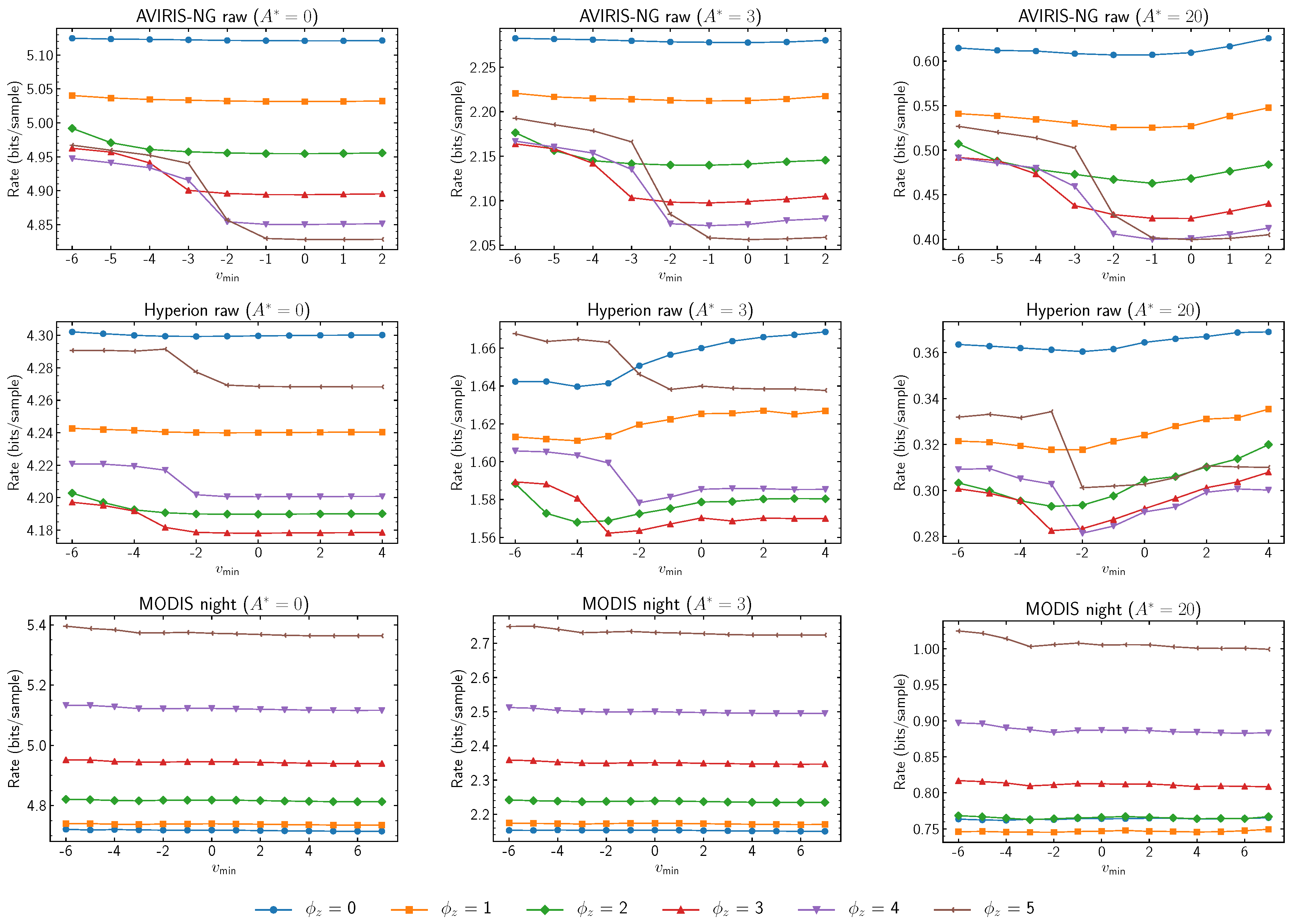
When damping values are examined in relation to ${\nu }_{\min }$ and ${\nu }_{\max }$ in Figure 5 and Figure 6, larger damping values have been found to be related to a decreased performance at higher ${\nu }_{\max }$ values. Setting ${\nu }_{\max }=7-2^{-\mathsf{\Theta }+3}{\varphi }_z$ has been found to be a good choice in the experimental results. Similarly, higher damping values seem to produce decreased performances when used with smaller ${\nu }_{\min }$ values. Thus, higher damping values seem to narrow the desirable predictor learning rates.

Figure 7 reports the relation between damping value ${\varphi }_z$ and the quantity of samples necessary to reach a steady predictor state, as controlled by $t_{\mathrm{inc}}$. Curiously, for the ${\nu }_{\min }$ and ${\nu }_{\max }$ values set as described above, varying ${\varphi }_z$ does not seem to influence the choice of $t_{\mathrm{inc}}$.

The offset parameter, ${\psi }_z$, also affects sample representative values, though this value has no effect when compression is lossless. For properly-selected values of ${\varphi }_z$, experimental results suggest setting ${\psi }_z=2^{\mathsf{\Theta }}-1$ is a reasonable default choice (Figure 8).

3.3. Weight Component Resolution and Register Size

The precision with which the predictor stores its weight vector (i.e., its internal state) is controlled by the weight component resolution parameter, $\mathsf{\Omega }$. Together with the register size parameter, R, both parameters regulate the bit depths required for the multipliers employed in the predictor calculation. For each multiplier, the value of $\mathsf{\Omega }$ controls the depth of one of its inputs (the other is controlled by image bit depth), while the value of R enables the multipliers to provide results modulo R, thus limiting its output bit depth.

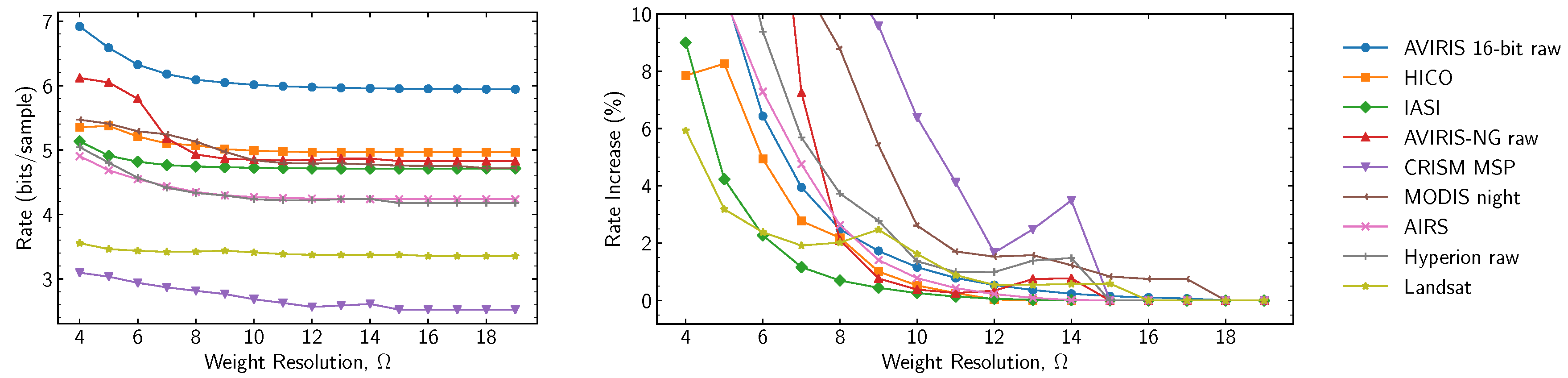
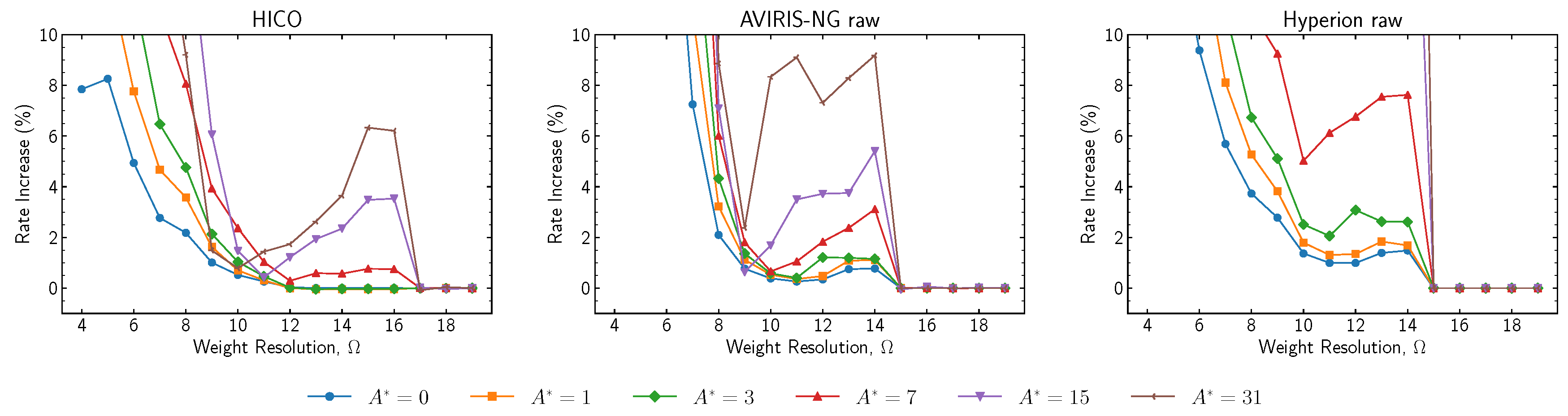
The effects of varying weight resolutions are reported in Figure 9 and Figure 10. For lossless compression, Figure 9 shows the relation between weight resolution and rate, both in absolute and relative terms. It can be observed that as $\mathsf{\Omega }$ is decreased, prediction accuracy is negatively impacted by less accurate weight vector coefficients, and thus, the rate is increased. For the images tested, weight resolution can be decreased down to 11 bits with a rate increase smaller than 5%. For near-lossless compression, Figure 10 shows the relation between weight resolution and rate increase over results for $\mathsf{\Omega }=19$. It can be observed that the small perturbations in the curves for $A^{*}=0$ are significantly amplified as $A^{*}$ increases. While the predictor is approximately linear, lower values of $\mathsf{\Omega }$ seem to magnify the non-linear interactions that finite-precision operations have on least significant bits.

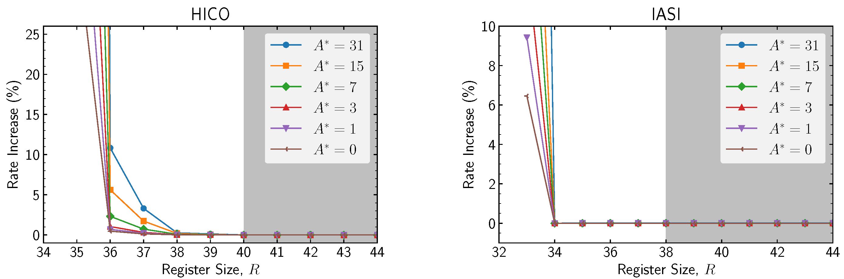
The effects of varying the register size parameter, R, are shown in Figure 11. For values of R over a certain threshold (shaded in gray in the figure plots), prediction results can be proven invariant [22] (pp. 4–7). While decreasing register size by one or two bits under this threshold does not increase the rate significantly, decreasing a few more bits rapidly yields very large increases in the rate.

3.4. Weight Exponent Offsets

The use of weight exponent offsets $\{{\zeta }_z^{\left(i\right)},{\zeta }^{*}\}$ allows fine tuning of the predictor learning rate for each band, and within a band for each predictor input as defined by the prediction mode and number of prediction bands. Hence, weight exponent offsets can be seen as an extension to the learning rate control provided through ${\nu }_{\min }$ and ${\nu }_{\max }$.

A brute force approach has been followed to understand the potential gains that could yield well-informed choices of weight exponent offsets for some of the corpus images. The procedure employed is as follows. First, optimal values for ${\nu }_{\min }$ and ${\nu }_{\max }$ are found through exhaustive search. Then, all choices of weight exponent offsets are tested for the first image band. The best choice is kept for that band, and the same procedure is repeated for each remaining band, one by one, until all weight exponent offsets are set.

Results are reported in

Table 4. Data reductions obtained for weight exponent offsets set through exhaustive search.

Image	Data Reduction (%)
AVIRIS Yellowstone Scene 0 raw	0.3%
Landsat Agriculture	0.2%
MODIS 500 m A2001123.0000	0.5%
Pleiades Montpellier Misreg0	0.1%
Vegetation 1 1b	0.3%

. When a fixed damping value is used for an entire image, as studied in this article, the potential coding performance gains obtained by weight exponent offsets are scant.

Nonetheless, given that good choices for ${\nu }_{\max }$ vary from instrument to instrument, it is foreseen that an end-user may want to adjust the predictor learning rate for each image band. In particular, the end-user may want to do so whenever different per-band noise profiles recommend the use of different per-band sample representative damping values, or for images with large signal energy variation among bands. The authors have observed gains of up to 7% in a synthetic scenario where an instrument with large energy variations is simulated. For this purpose, a synthetic image is produced from a high SNR image by simulating 32 consecutive very dark bands followed by 32 consecutive very bright bands. Gains are observed when the synthetic image is encoded with band-dependent absolute error limits so that both dark and bright bands are encoded at roughly 1.5 bits per sample. However, setting per-band damping values requires a careful instrument modeling, which is out of the scope of this article.

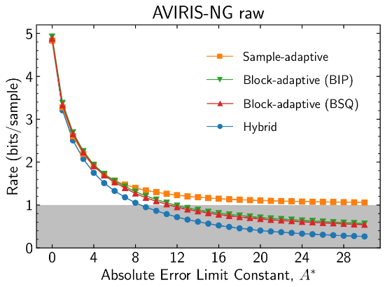
3.5. Entropy Encoder

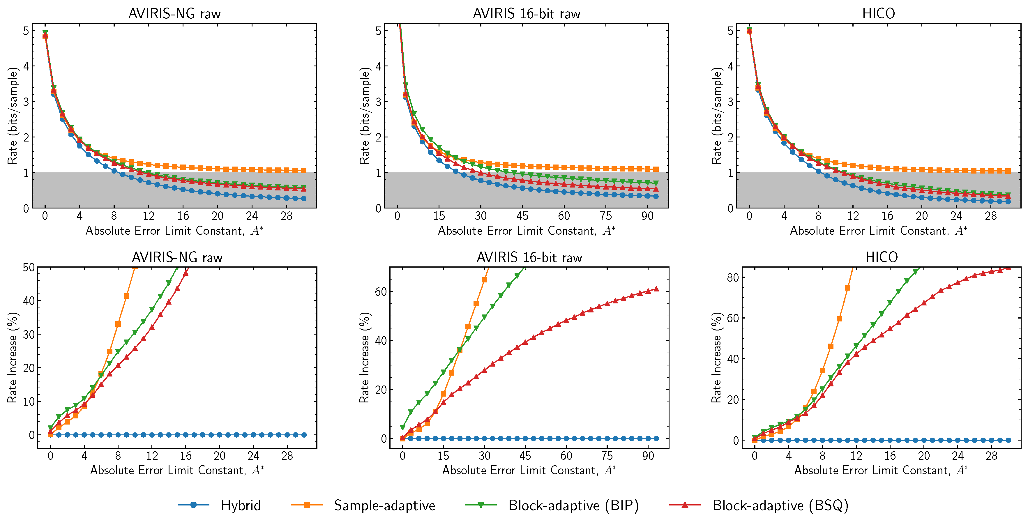
Issue 2 incorporates a new hybrid entropy encoder in addition to the sample-adaptive and block-adaptive encoders available in Issue 1. At high rates, the hybrid encoder encodes most samples using a family of codes that are equivalent to those used by the sample-adaptive coder, and thus has nearly identical performance [22]. However, the hybrid encoder has substantially better performance than the Issue 1 entropy encoders at low bit rates (Figure 12).

The sample-adaptive encoder is unable to reach rates lower than 1 bit per sample (due to design constraints), whereas the block-adaptive encoder is able to do so, but with non-negligible rate overhead over the hybrid encoder. In addition, the block-adaptive encoder may have poor performance when encoding in band interleaved by pixel (BIP) order, because samples from different bands (which may have different statistical behavior) are jointly encoded in the same block. Setting encoding order to band sequential (BSQ) encoding order somewhat mitigates these issues. However, the use of BSQ encoding order may not be suitable for all instruments due to large buffering requirements when acquisition order is not BSQ. In this case, similar performance may be often obtained by band interleaved by line (BIL) encoding order (Figure 13).

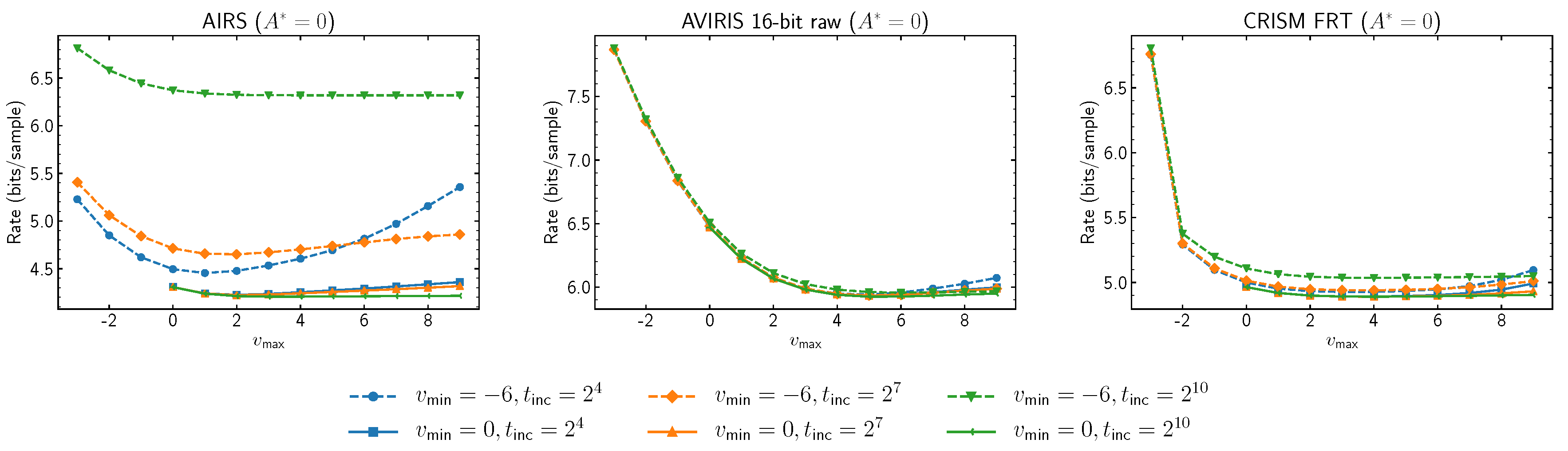
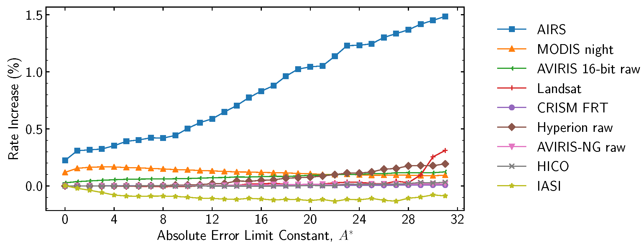
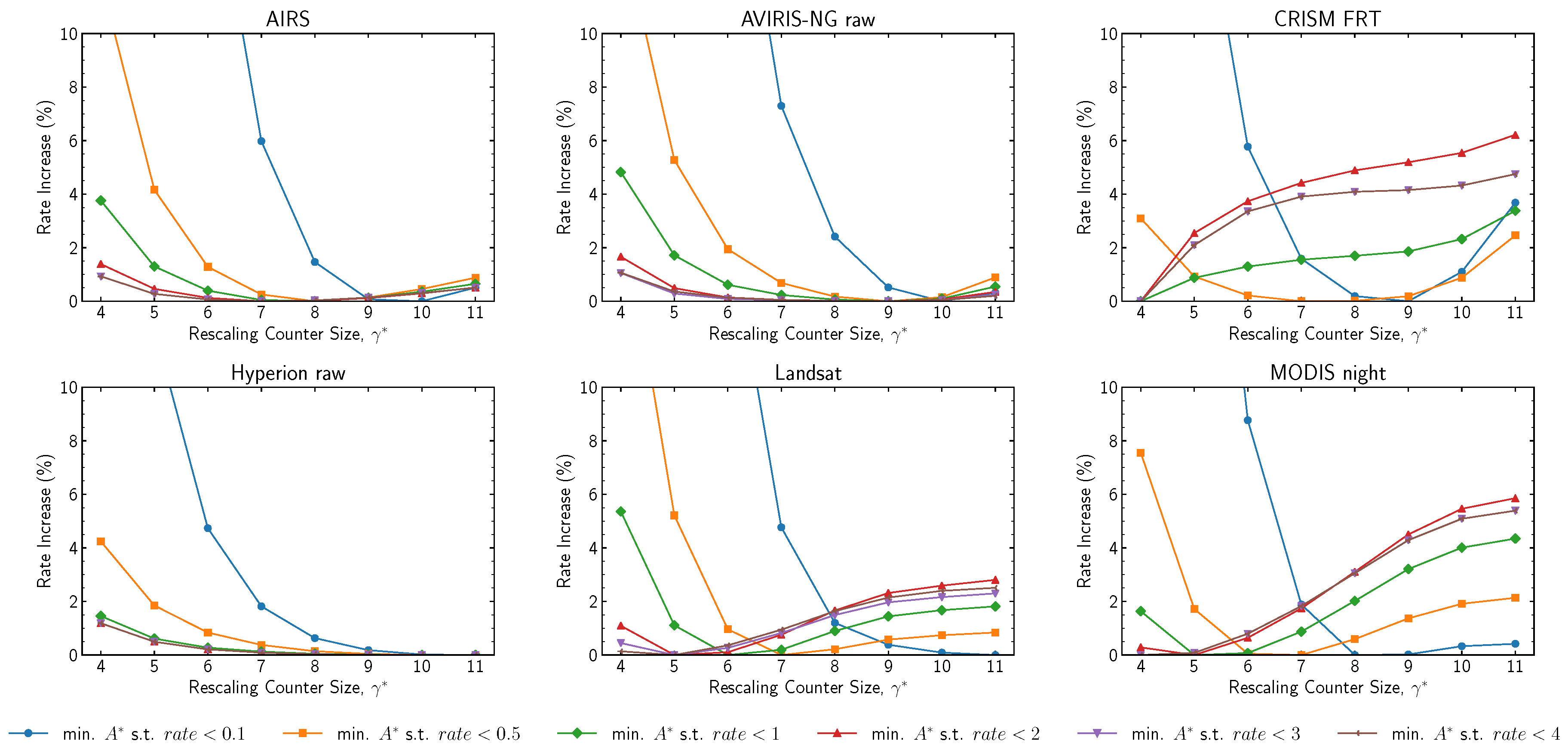
Code selection statistics used by the hybrid entropy coder are periodically rescaled at an interval determined by parameter ${\gamma }^{*}$; this is the parameter that has the most significant impact on hybrid entropy coder performance. Within each band, each time rescaling occurs, an additional bit is output to the compressed bitstream so that the decompressor can reconstruct the code selection statistics. At lower bit rates, this overhead can become significant, and larger values of ${\gamma }^{*}$ are required to diminish its impact. This can be seen in Figure 14, where ${\gamma }^{*}$ is varied. Results are reported in relation to the obtained data rate by adjusting the absolute error limit constant $A^{*}$ (via trial-and-error) to achieve bit rates of approximately $0.1$, $0.5$, 1, 2, 3, and 4 bits per sample for the optimal ${\gamma }^{*}$ value.

The results suggest the use of ${\gamma }^{*}\approx 6$ for a high rate and to transition to larger ${\gamma }^{*}$ values at rates below 1 bit per sample. At high compressed data rates, these results are comparable to those for the sample-adaptive encoder due to their similar operation. Inflection points are due to the logarithmic nature of the parameter, where a one-unit increase doubles the size of the renormalization interval and makes local statistics less important to the entropy encoder. For instance, this explains the CRISM FRT plot, where the results tend to stabilize as ${\gamma }^{*}$ grows.

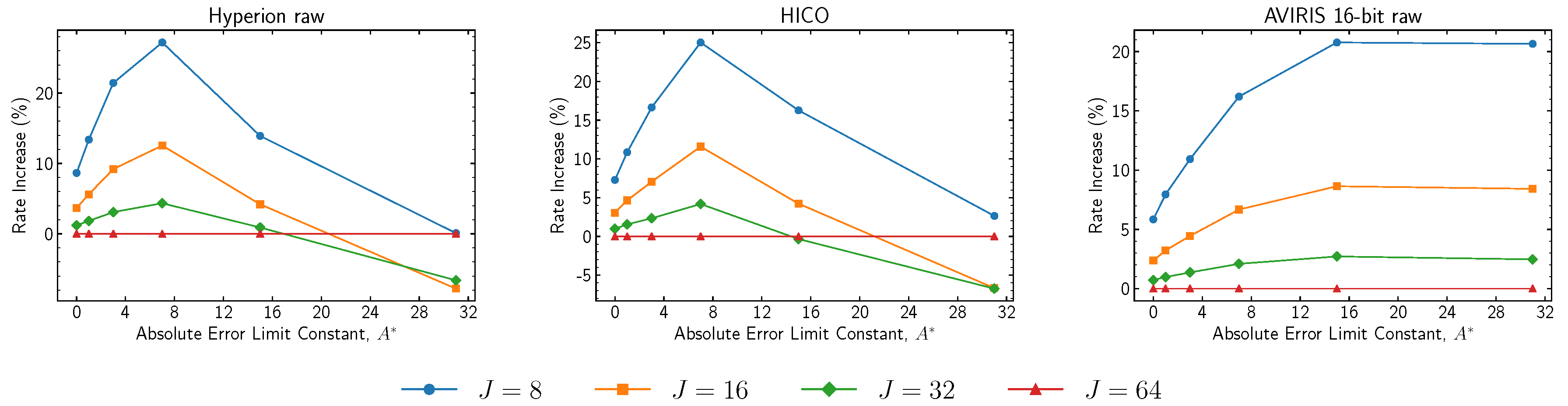
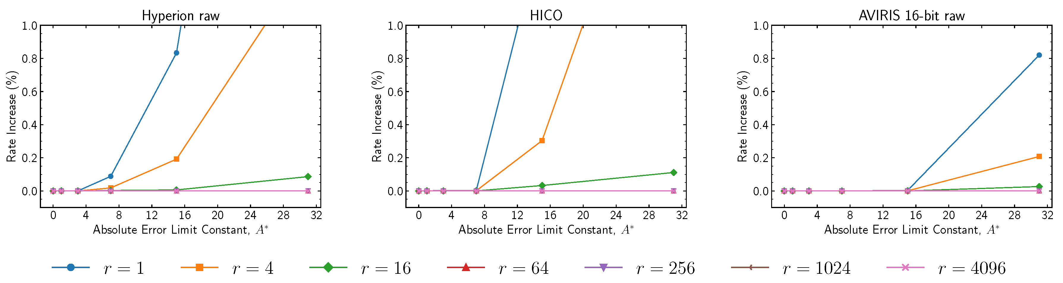
Results regarding the operation of the block-adaptive encoder under near-lossless mode for high compressed data rates are now reported. The encoder operation is controlled by the reference sample interval parameter, r, and the block size parameter, J, with results reported respectively in Figure 15 and Figure 16. The reference sample interval enables efficient encoding of “zero-block” runs (sequences of blocks of zero values). However, the practical effects of this parameter are negligible except for combinations of very small values of r with high values of $A^{*}$. Regarding the block size values, for small absolute error limit constant values, where it makes sense to use the block-adaptive encoder, employing a block size of 64 yields better performance, even if this trend is reversed for larger $A^{*}$ values.

4. Conclusions

This article examined performance trade-offs among key parameters and options in the new Issue 2 of “Low-Complexity Lossless and Near-Lossless Multispectral and Hyperspectral Image Compression.”

The behavior of the new near-lossless capability was studied along with the effects of four key new features: narrow local sums, sample representatives, weight exponent offsets, and the new hybrid entropy encoder.

Regarding narrow local sums, their use tends to incur a minimal to moderate coding performance penalty. In particular, this penalty tends to be fairly small for column-oriented local sums when image height is large.

In the study of sample representatives, for many images, well-chosen nonzero values of parameters ${\varphi }_z$ and ${\psi }_z$ were shown to provide a noticeable improvement in compression performance compared to the obvious alternative of setting the sample representative equal to the center of the quantizer bin (achieved by setting ${\varphi }_z={\psi }_z=0$). However, at larger values of ${\varphi }_z$, performance becomes more sensitive to prediction adaptation rates as controlled though ${\nu }_{\min }$ and ${\nu }_{\max }$. It is recommended to decrease ${\nu }_{\max }$ as ${\varphi }_z$ increases.

Concerning the use of weight exponent offsets, for the images tested in this article and in combination with band-independent sample representative parameters, the use of nonzero weight exponent offsets has shown scant performance increments. The significant band-to-band variation in signal energy needed to motivate the use of nonzero weight exponent offsets may be uncommon in practice, based on the images in the corpus.

Regarding the variables controlling data widths in the predictor, the recommended value for $\mathsf{\Omega }$ is 19 bits. For very small absolute error limits, this value can be lowered down to 11 bits with a rate increase of less than 5% for the images tested. Parameter R can be set one or two bits below the proven invariance threshold at insignificant rate variations. Setting values larger than necessary yields no benefits.

Finally, under near-lossless compression, the hybrid entropy encoder has shown substantial coding gains compared to the legacy coding options, particularly as the maximum allowed error increases. Experimental results suggest that higher values of ${\gamma }^{*}$ improve performance at lower bit rates. Regarding the block-adaptive entropy encoder, larger block sizes have been shown to yield improved coding performances when the maximum allowed error was small.

References

- Motta, G.; Rizzo, F.; Storer, J.A. Hyperspectral Data Compression; Springer Science & Business Media: New York, NY, USA, 2006. [Google Scholar]
- Blanes, I.; Serra-Sagrista, J.; Marcellin, M.W.; Bartrina-Rapesta, J. Divide-and-conquer strategies for hyperspectral image processing: A review of their benefits and advantages. IEEE Signal Process. Mag. 2012, 29, 71–81. [Google Scholar] [CrossRef]
- Báscones, D.; González, C.; Mozos, D. Hyperspectral Image Compression Using Vector Quantization, PCA and JPEG2000. Remote Sens. 2018, 10, 907. [Google Scholar] [CrossRef]
- Consultative Committee for Space Data Systems. Lossless Data Compression. Recommendation for Space Data System Standards, CCSDS 121.0-B-2; CCSDS: Washington, DC, USA, 2012. [Google Scholar]
- Consultative Committee for Space Data Systems. Image Data Compression. Recommendation for Space Data System Standards, CCSDS 122.0-B-2; CCSDS: Washington, DC, USA, 2017. [Google Scholar]
- Consultative Committee for Space Data Systems. Spectral Preprocessing Transform for Multispectral and Hyperspectral Image Compression. Recommendation for Space Data System Standards, CCSDS 122.1-B-1; CCSDS: Washington, DC, USA, 2017. [Google Scholar]
- Consultative Committee for Space Data Systems. Lossless Multispectral & Hyperspectral Image Compression. Recommendation for Space Data System Standards, CCSDS 123.0-B-1; CCSDS: Washington, DC, USA, 2012. [Google Scholar]
- Consultative Committee for Space Data Systems. Lossless and Near-Lossless Multispectral and Hyperspectral Image Compression. Recommendation for Space Data System Standards, CCSDS 123.0-B-2; CCSDS: Washington, DC, USA, 2019. [Google Scholar]
- Klimesh, M. Low-complexity adaptive lossless compression of hyperspectral imagery. Proc. SPIE 2006, 6300, 63000N-1–63000N-9. [Google Scholar]
- Klimesh, M.; Kiely, A.; Yeh, P. Fast lossless compression of multispectral and hyperspectral imagery. In Proceedings of the 2nd International WS on On-Board Payload Data Compression (OBPDC), ESA/CNES, Tolouse, France, 28–29 October 2010. [Google Scholar]
- Keymeulen, D.; Aranki, N.; Bakhshi, A.; Luong, H.; Sarture, C.; Dolman, D. Airborne demonstration of FPGA implementation of Fast Lossless hyperspectral data compression system. In Proceedings of the 2014 IEEE NASA/ESA Conference on Adaptive Hardware and Systems (AHS), Leicester, UK, 14–18 July 2014; pp. 278–284. [Google Scholar]
- Santos, L.; Berrojo, L.; Moreno, J.; López, J.F.; Sarmiento, R. Multispectral and hyperspectral lossless compressor for space applications (HyLoC): A low-complexity FPGA implementation of the CCSDS 123 standard. IEEE J. Sel. Top. Appl. Earth Obs. Remote Sens. 2016, 9, 757–770. [Google Scholar] [CrossRef]
- Theodorou, G.; Kranitis, N.; Tsigkanos, A.; Paschalis, A. High performance CCSDS 123.0-B-1 multispectral & hyperspectral image compression implementation on a space-grade SRAM FPGA. In Proceedings of the 5th International Workshop On-Board Payload Data Compression, Frascati, Italy, 28–29 September 2016; pp. 28–29. [Google Scholar]
- Báscones, D.; González, C.; Mozos, D. FPGA implementation of the CCSDS 1.2. 3 standard for real-time hyperspectral lossless compression. IEEE J. Sel. Top. Appl. Earth Obs. Remote Sens. 2018, 11, 1158–1165. [Google Scholar] [CrossRef]
- Báscones, D.; González, C.; Mozos, D. Parallel Implementation of the CCSDS 1.2. 3 Standard for Hyperspectral Lossless Compression. Remote Sens. 2017, 9, 973. [Google Scholar] [CrossRef]
- Tsigkanos, A.; Kranitis, N.; Theodorou, G.A.; Paschalis, A. A 3.3 Gbps CCSDS 123.0-B-1 multispectral & Hyperspectral image compression hardware accelerator on a space-grade SRAM FPGA. IEEE Trans. Emerg. Top. Comput. 2018. [Google Scholar] [CrossRef]
- Fjeldtvedt, J.; Orlandić, M.; Johansen, T.A. An efficient real-time FPGA implementation of the CCSDS-123 compression standard for hyperspectral images. IEEE J. Sel. Top. Appl. Earth Obs. Remote Sens. 2018, 11, 3841–3852. [Google Scholar] [CrossRef]
- Orlandić, M.; Fjeldtvedt, J.; Johansen, T.A. A Parallel FPGA Implementation of the CCSDS-123 Compression Algorithm. Remote Sens. 2019, 11, 673. [Google Scholar] [CrossRef]
- Rodríguez, A.; Santos, L.; Sarmiento, R.; Torre, E.D.L. Scalable Hardware-Based On-Board Processing for Run-Time Adaptive Lossless Hyperspectral Compression. IEEE Access 2019, 7, 10644–10652. [Google Scholar] [CrossRef]
- Kiely, A.; Klimesh, M.; Blanes, I.; Ligo, J.; Magli, E.; Aranki, N.; Burl, M.; Camarero, R.; Cheng, M.; Dolinar, S.; et al. The new CCSDS standard for low-complexity lossless and near-lossless multispectral and hyperspectral image compression. In Proceedings of the 6th International WS on On-Board Payload Data Compression (OBPDC), ESA/CNES, Matera, Italy, 20–21 September 2018. [Google Scholar]
- Augé, E.; Sánchez, J.E.; Kiely, A.; Blanes, I.; Serra-Sagristà, J. Performance impact of parameter tuning on the CCSDS-123 lossless multi- and hyperspectral image compression standard. J. Appl. Remote Sens. 2013, 7. [Google Scholar] [CrossRef]
- Consultative Committee for Space Data Systems. Lossless Multispectral & Hyperspectral Image Compression. Report Concerning Space Data System Standards, CCSDS 120.2-G-1; CCSDS: Washington, DC, USA, 2012. [Google Scholar]
- Consultative Committee for Space Data Systems. Testing and Evaluation Image Corpus of CCSDS-123.0-B-1. Available online: https://cwe.ccsds.org/sls/docs/SLS-DC/123.0-B-Info/TestData/ (accessed on 10 June 2019).
- Valsesia, D.; Magli, E. A Novel Rate Control Algorithm for Onboard Predictive Coding of Multispectral and Hyperspectral Images. IEEE Trans. Geosci. Remote Sens. 2014, 52, 6341–6355. [Google Scholar] [CrossRef] [Green Version]
- Conoscenti, M.; Coppola, R.; Magli, E. Constant SNR, Rate Control, and Entropy Coding for Predictive Lossy Hyperspectral Image Compression. IEEE Trans. Geosci. Remote Sens. 2016, 54, 7431–7441. [Google Scholar] [CrossRef]
Figure 1.
Compressed bit rate for different choices of prediction mode and local sum type. Plots in the left column are for lossless compression (
). Plots in the right column are relative to the adjusted combination of the local sum type and prediction mode described in
Section 2.
Figure 2.
Average compressed bit rate performance as a function of P.
Figure 3.
Average compressed data rate as a function of when and .
Figure 4.
Average compressed data rate for different choices of parameters that affect the adaptation of the predictor to the image.
Figure 5.
Average compressed data rate as a function of for different values of the sample representative damping value, , and absolute error limit constant , when .
Figure 6.
Average compressed data rate as a function of for various values of the sample representative damping value, , and absolute error limit constant, , when .
Figure 7.
Figure 8.
Average compressed data rate as a function of for various values of sample representative damping value and absolute error limit constant , when .
Figure 9.
Average bit rate as a function of weight resolution for lossless compression (). Curves in the right plot are relative to .
Figure 10.
Change in the compressed data rate as a function of weight resolution (and relative to ) for multiple absolute error limit constants .
Figure 11.
Change in compressed data rate as a function of register size R for multiple absolute error limit constants . Results are relative to .
Figure 12.
Compressed data rate for each entropy encoder as a function of absolute error limit constant as the absolute value (top) and relative increases over the hybrid entropy encoder (bottom). Parameters for the sample-adaptive encoder are , , and . Parameters for the block-adaptive encoder are and .
Figure 13.
Change in compressed data rate for the block-adaptive entropy encoder when encoding in BIL order relative to when encoding in BSQ order. Parameters for the block-adaptive encoder are and .
Figure 14.
Change in compressed data rate (i.e., relative to an optimal selection of ) as a function of rescaling counter size .
Figure 15.
Average compressed data rate when employing the block-adaptive entropy encoder as a function of absolute error limit constant . Results are relative to . Block size J is set to 64, and images are encoded in BIL order.
Figure 16.
Change in compressed data rate when employing the block-adaptive entropy encoder for multiple block sizes J as a function of absolute error limit constant . Results are relative to . Reference sample interval r is set to 4096, and images are encoded in BIL order.