Contrasting the Performance of Eight Satellite-Based GPP Models in Water-Limited and Temperature-Limited Grassland Ecosystems

 ,
, 
Abstract
1. Introduction
2. Materials and Methods
2.1. Model Overview
2.1.1. The Vegetation Photosynthesis Model (VPM)
2.1.2. The Modified VPM (MVPM)
2.1.3. The MODIS GPP Algorithm (MODIS-GPP)
2.1.4. The Temperature and Greenness model (TG)
2.1.5. The Greenness and Radiation Model (GR)
2.1.6. The Vegetation Index Model (VI)
2.1.7. The Alpine Vegetation Model (AVM)
2.1.8. The Photosynthetic Capacity Model (PCM)
2.2. Data
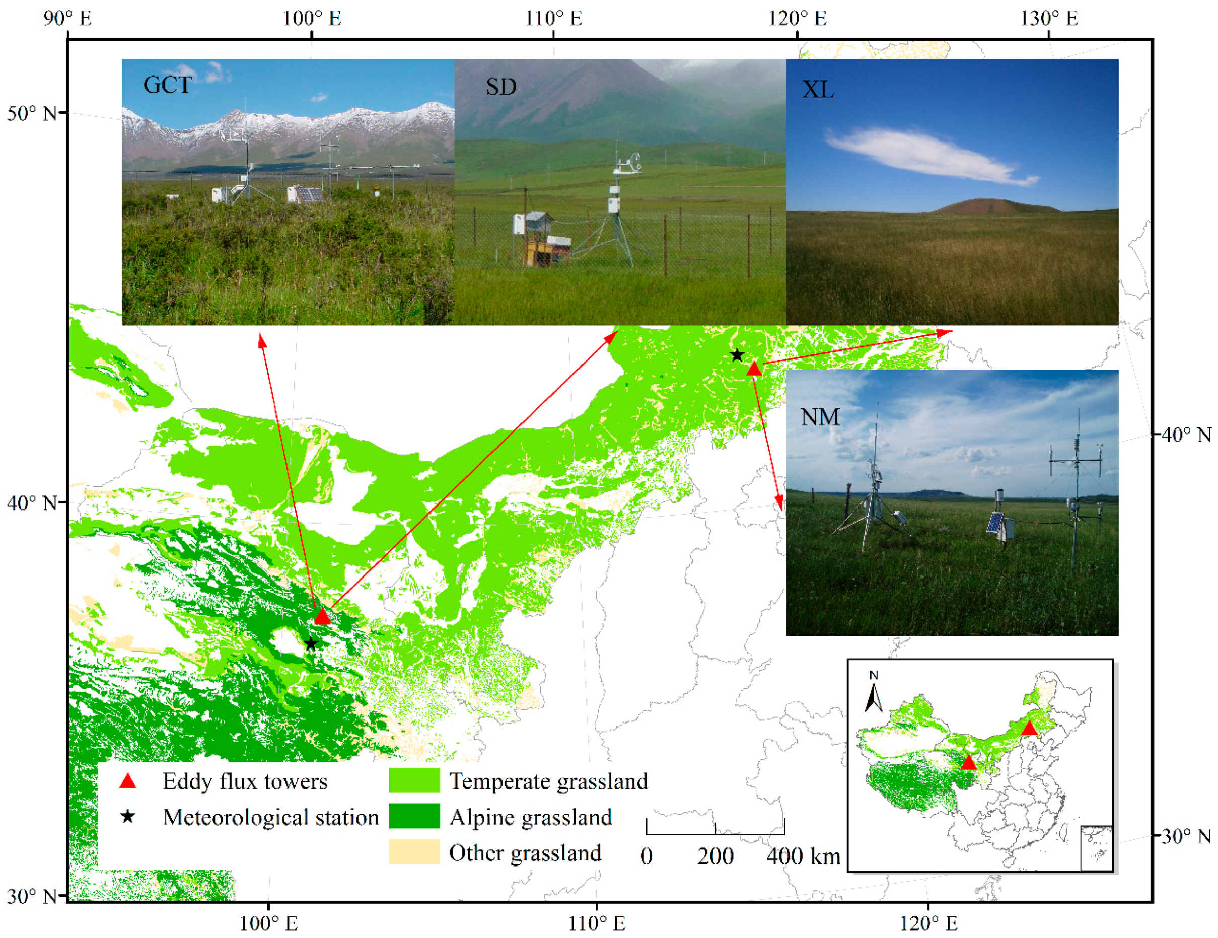
2.2.1. Study Sites
2.2.2. GPP and Meteorological Data
2.2.3. MODIS Products
2.3. Model Calibration
2.4. Evaluation of Model Performance
3. Results
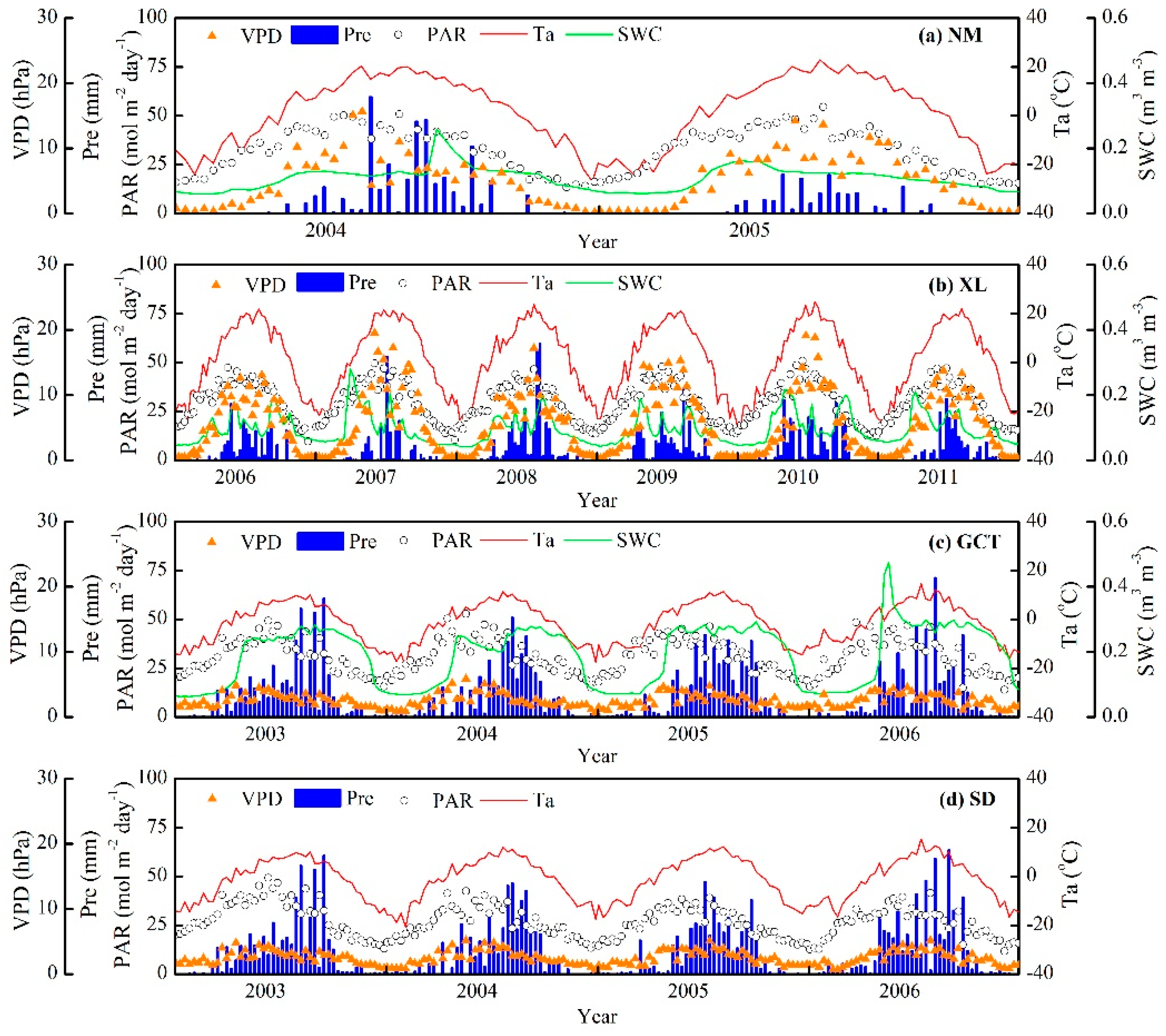
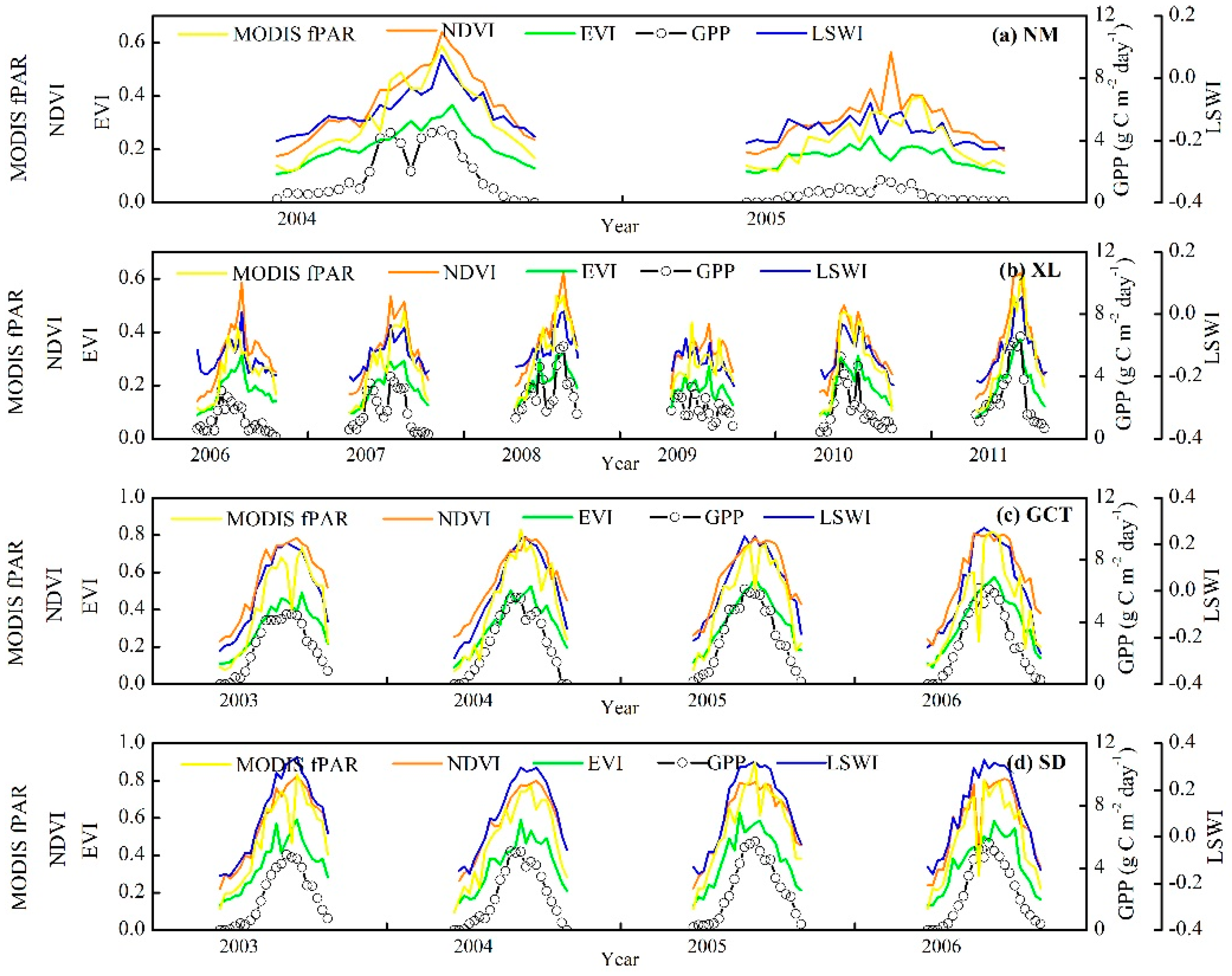
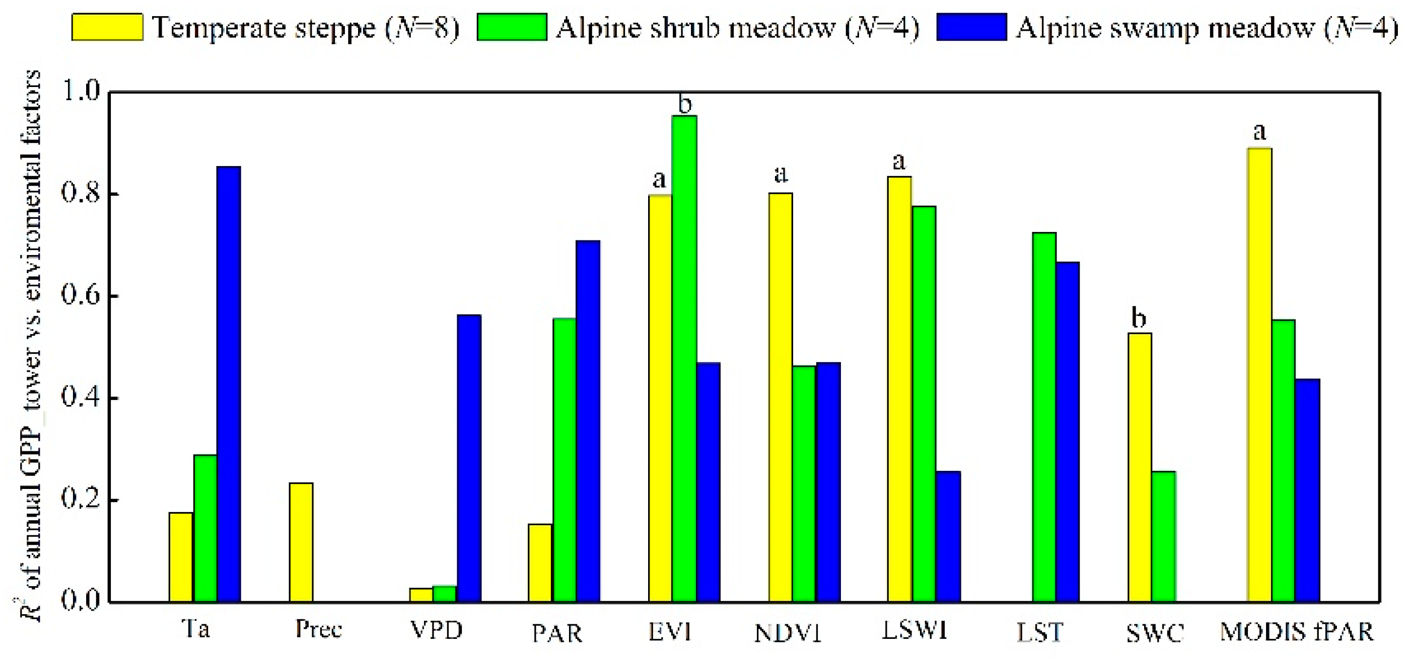
3.1. Seasonal and Interannual Variations in Climate, GPP, and Vegetation Indices at the Four Flux Tower Sites
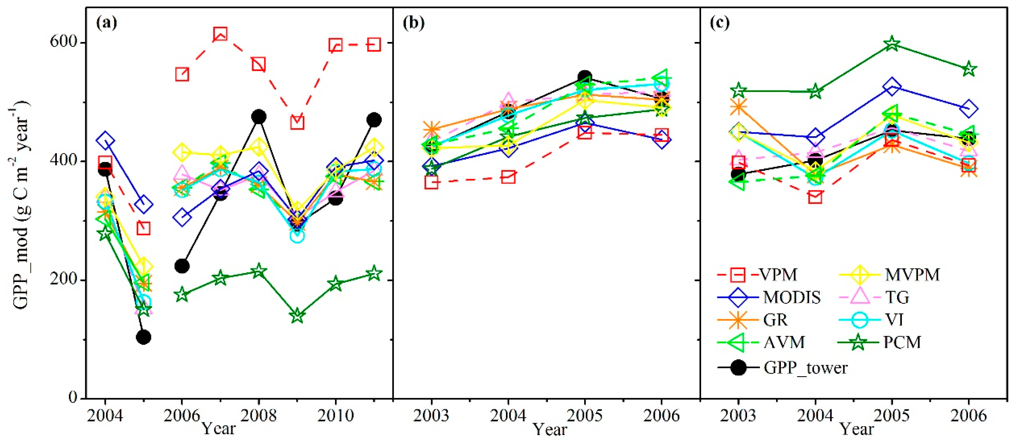
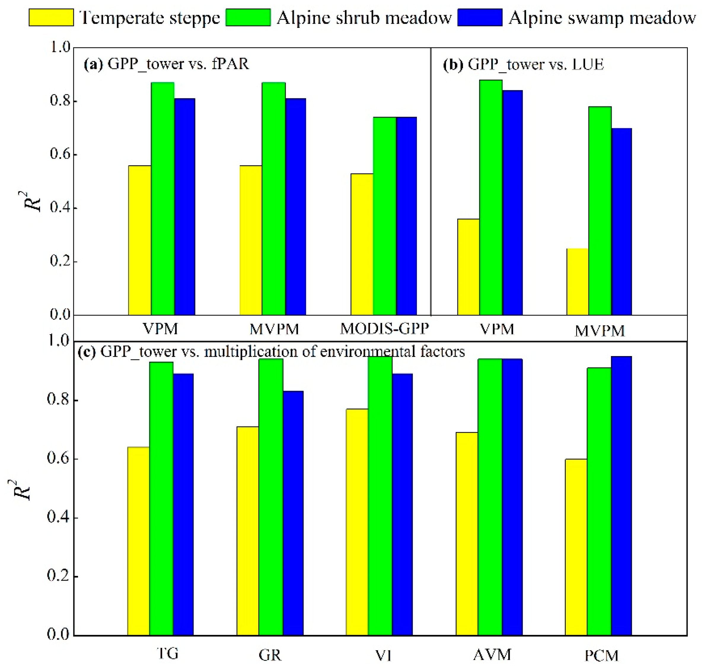
3.2. Comparison of the Eight Satellite-Based GPP Models in Estimating GPP between the Temperate Steppe and Alpine Meadow
4. Discussion
4.1. Varying Performances of the Eight Satellite-Based GPP Models between the Temperate Steppe and Alpine Meadow
4.2. Varying Performances of the Eight Satellite-Based GPP Models in the Temperate Steppe
4.3. Varying Performances of the Eight Satellite-Based GPP Models in the Alpine Meadow
4.4. Comparisons with Previous Studies on Grassland
4.5. Trade-Offs between Model Performance and Applicability at a Regional Scale
5. Conclusions
Author Contributions
Funding
Acknowledgments
Conflicts of Interest
Abbreviations
| EC | Eddy covariance |
| PPFD | Photosynthetic photon flux density |
| NEE | Net ecosystem CO2 exchange |
| Re | Ecosystem respiration |
| GPP | Gross primary productivity |
| VPM | Vegetation photosynthesis model |
| MVPM | Modified VPM model |
| MODIS-GPP | Moderate Resolution Imaging Spectroradiometer GPP algorithm |
| TG | Temperature and greenness model |
| GR | Greenness and radiation model |
| VI | Vegetation index model |
| AVM | Alpine vegetation model |
| PCM | Photosynthetic Capacity Model |
| LUE | Light use efficiency |
| εmax | Potential LUE without environmental stress |
| εg | Actual LUE |
| ft | Effects of air temperature on εmax |
| fw | Effects of water availability on εmax |
| m | Slope between GPP and environmental scalars |
| PAR | Photosynthetically active radiation |
| fPAR | Fraction of PAR absorbed by the vegetation canopy |
| Ta | Air temperature |
| VPD | Vapor pressure deficit |
| EVI | Enhanced vegetation index |
| LSWI | Land surface water index |
| LST | Land surface temperature |
| LSTan | Mean annual nighttime LST |
References
- Chapin, F.S., III; Matson, P.A.; Mooney, H.A. Principles of Terrestrial Ecosystem Ecology; Springer: New York, NY, USA, 2002; pp. 369–397. [Google Scholar]
- Yuan, W.; Liu, S.; Yu, G.; Bonnefond, J.M.; Chen, J.; Davis, K.; Desai, A.R.; Goldstein, A.H.; Gianelle, D.; Rossi, F. Global estimates of evapotranspiration and gross primary production based on modis and global meteorology data. Remote Sens. Environ. 2010, 114, 1416–1431. [Google Scholar] [CrossRef]
- Jia, W.; Liu, M.; Wang, D.; He, H.; Shi, P.; Li, Y.; Wang, Y. Uncertainty in simulating regional gross primary productivity from satellite-based models over northern china grassland. Ecol. Indic. 2018, 88, 134–143. [Google Scholar] [CrossRef]
- Li, Z.; Yu, G.; Xiao, X.; Li, Y.; Zhao, X.; Ren, C.; Zhang, L.; Fu, Y. Modeling gross primary production of alpine ecosystems in the tibetan plateau using modis images and climate data. Remote Sens. Environ. 2007, 107, 510–519. [Google Scholar] [CrossRef]
- Liu, D.; Li, Y.; Wang, T.; Peylin, P.; Macbean, N.; Ciais, P.; Jia, G.; Ma, M.; Ma, Y.; Shen, M. Contrasting responses of grassland water and carbon exchanges to climate change between tibetan plateau and inner Mongolia. Agric. For. Meteorol. 2018, 249, 163–175. [Google Scholar] [CrossRef]
- Baldocchi, D. Measuring fluxes of trace gases and energy between ecosystems and the atmosphere - the state and future of the eddy covariance method. Glob. Change Biol. 2014, 20, 3600–3609. [Google Scholar] [CrossRef] [PubMed]
- Schmid, H.P. Source areas for scalars and scalar fluxes. Bound.-Lay. Meteorol. 1994, 67, 293–318. [Google Scholar] [CrossRef]
- Wu, C.; Niu, Z.; Gao, S. Gross primary production estimation from modis data with vegetation index and photosynthetically active radiation in maize. J. Geophys. Rese. Atmos. 2010, 115, D12127. [Google Scholar] [CrossRef]
- Zhang, L.X.; Zhou, D.C.; Fan, J.W.; Hu, Z.M. Comparison of four light use efficiency models for estimating terrestrial gross primary production. Ecol. Modell. 2015, 300, 30–39. [Google Scholar] [CrossRef]
- Keenan, T.F.; Baker, I.; Barr, A.; Ciais, P.; Davis, K.; Dietze, M.; Dragoni, D.; Gough, C.M.; Grant, R.; Hollinger, D. Terrestrial biosphere model performance for inter-annual variability of land-atmosphere CO2 exchange. Glob. Change Biol. 2012, 18, 1971–1987. [Google Scholar] [CrossRef]
- Ruimy, A.; Bondeau, L.K. Comparing global models of terrestrial net primary productivity (NPP): Analysis of differences in light absorption and light-use efficiency. Glob. Change Biol. 1999, 5, 56–64. [Google Scholar] [CrossRef]
- Running, S.W.; Coughlan, J.C. A General model of forest ecosystem processes for regional applications i. hydrologic balance, canopy gas exchange and primary production processes. Ecol. Modell. 1988, 42, 125–154. [Google Scholar] [CrossRef]
- Cramer, W.; Kicklighter, D.W.; Bondeau, A.; Iii, B.M.; Churkina, G.; Nemry, B.; Ruimy, A.; Schloss, A.L.; ThE. Participants OF. ThE. Potsdam NpP. Model Intercomparison. Comparing global models of terrestrial net primary productivity (NPP): Overview and key results. Glob. Change Biol. 1999, 5, 1–15. [Google Scholar] [CrossRef]
- Cramer, W.; Bondeau, A.; Woodward, F.I.; Prentice, I.C.; Betts, R.A.; Brovkin, V.; Cox, P.M.; Fisher, V.; Foley, J.A.; Friend, A.D.; et al. Global response of terrestrial ecosystem structure and function to CO2 and climate change: Results from six dynamic global vegetation models. Glob. Change Biol. 2001, 7, 357–373. [Google Scholar] [CrossRef]
- Knorr, W.; Heimann, M. Uncertainties in global terrestrial biosphere modeling: 1. A comprehensive sensitivity analysis with a new photosynthesis and energy balance scheme. Global Biogeochem. Cy. 2001, 15, 207–225. [Google Scholar] [CrossRef]
- Raupach, M.R.; Rayner, P.J.; Barrett, D.J.; DeFries, R.S.; Heimann, M.; Ojima, D.S.; Quegan, S.; Schmullius, C.C. Model–Data synthesis in terrestrial carbon observation: Methods, data requirements and data uncertainty specifications. Glob. Change Biol. 2005, 11, 378–397. [Google Scholar] [CrossRef]
- Yuan, W.; Cai, W.; Xia, J.; Chen, J.; Liu, S.; Dong, W.; Merbold, L.; Law, B.; Arain, A.; Beringer, J. Global comparison of light use efficiency models for simulating terrestrial vegetation gross primary production based on the LaThuile database. Agric. For. Meteorol. 2014, 192–193, 108–120. [Google Scholar] [CrossRef]
- Dong, J.; Xiao, X.; Wagle, P.; Zhang, G.; Zhou, Y.; Jin, C.; Torn, M.S.; Meyers, T.P.; Suyker, A.E.; Wang, J. Comparison of four evi-based models for estimating gross primary production of maize and soybean croplands and tallgrass prairie under severe drought. Remote Sens. Environ. 2015, 162, 154–168. [Google Scholar] [CrossRef]
- Monteith, J.L. Solar radiation and productivity in tropical ecosystems. J. Appl. Ecol. 1972, 9, 747–766. [Google Scholar] [CrossRef]
- Monteith, J.L. Climate and the efficiency of crop production in britain. Philos. Trans. Royal Soc. Biol. Sci. 1977, 281, 277–294. [Google Scholar] [CrossRef]
- Potter, C.S.; Randerson, J.T.; Field, C.B.; Matson, P.A.; Vitousek, P.M.; Mooney, H.A.; Klooster, S.A. Terrestrial ecosystem production: A process model based on global satellite and surface data. Global Biogeochem. Cy. 1993, 7, 811–841. [Google Scholar] [CrossRef]
- Prince, S.D.; Goward, S.N. Global primary production: A remote sensing approach. J. Biogeography 1995, 22, 815–835. [Google Scholar] [CrossRef]
- Running, S.W.; Nemani, R.; Glassy, J.M.; Thornton, P.E. MODIS daily photosynthesis (PSN) and annual net primary production (NPP) product (MOD17) algorithm theoretical basis document. 2015. Available online: www. ntsg. umt. edu/modis/ATBD/ATBD_MOD17_v21. pdf (accessed on 1 March 2018).
- Running, S.W.; Thornton, P.E.; Nemani, R.; Glassy, J.M. Global terrestrial gross and net primary productivity from the earth observing system. In Methods in Ecosystem Science; Springer: New York, NY, USA, 2000; pp. 44–57. [Google Scholar]
- Xiao, X.; Hollinger, D.; Aber, J.; Goltz, M.; Davidson, E.A.; Zhang, Q.; Iii, B.M. Satellite-based modeling of gross primary production in an evergreen needleleaf forest. Remote Sens. Environ. 2004, 89, 519–534. [Google Scholar] [CrossRef]
- Xiao, X.; Zhang, Q.; Braswell, B.; Urbanski, S.; Boles, S.; Wofsy, S.; Iii, B.M.; Ojima, D. Modeling gross primary production of temperate deciduous broadleaf forest using satellite images and climate data. Remote Sens. Environ. 2004, 91, 256–270. [Google Scholar] [CrossRef]
- Yuan, W.; Liu, S.; Zhou, G.; Zhou, G.; Tieszen, L.L.; Baldocchi, D.; Bernhofer, C.; Gholz, H.; Goldstein, A.H.; Goulden, M.L. Deriving a light use efficiency model from eddy covariance flux data for predicting daily gross primary production across biomes. Agric. For. Meteorol. 2007, 143, 189–207. [Google Scholar] [CrossRef]
- Sims, D.A.; Rahman, A.F.; Cordova, V.D.; El-Masri, B.Z.; Baldocchi, D.D.; Bolstad, P.V.; Flanagan, L.B.; Goldstein, A.H.; Hollinger, D.Y.; Misson, L. A new model of gross primary productivity for north american ecosystems based solely on the enhanced vegetation index and land surface temperature from MODIS. Remote Sens. Environ. 2008, 112, 1633–1646. [Google Scholar] [CrossRef]
- Gitelson, A.A.; Viña, A.; Verma, S.B.; Rundquist, D.C.; Arkebauer, T.J.; Keydan, G.; Leavitt, B.; Ciganda, V.; Burba, G.G.; Suyker, A.E. Relationship between gross primary production and chlorophyll content in crops: Implications for the synoptic monitoring of vegetation productivity. J. Geophys. Res. Atmosp. 2006, 111, D08S11. [Google Scholar] [CrossRef]
- Gulbeyaz, O.; Bond-Lamberty, B.; Akyurek, Z.; West, T.O. A New Approach to evaluate the MODIS annual NPP product (MOD17A3) using forest field data from Turkey. Int. J. Remote Sens. 2018, 39, 2560–2578. [Google Scholar] [CrossRef]
- Turner, D.P.; Ritts, W.D.; Cohen, W.B.; Gower, S.T.; Running, S.W.; Zhao, M.; Costa, M.H.; Kirschbaum, A.A.; Ham, J.M.; Saleska, S.R. Evaluation of MODIS NPP and GPP products across multiple biomes. Remote Sens. Environ. 2006, 102, 282–292. [Google Scholar] [CrossRef]
- Sims, D.A.; Rahman, A.F.; Cordova, V.D.; El-Masri, B.Z.; Baldocchi, D.D.; Flanagan, L.B.; Goldstein, A.H.; Hollinger, D.Y.; Misson, L.; Monson, R.K. On the use of MODIS EVI to assess gross primary productivity of north American ecosystems. J. Geophys. Res. Biogeosci. 2006, 111, 695–702. [Google Scholar] [CrossRef]
- Li, F.; Wang, X.; Zhao, J.; Zhang, X.; Zhao, Q. A Method for estimating the gross primary production of alpine meadows using modis and climate data in china. Inter. J. Remote Sens. 2013, 34, 8280–8300. [Google Scholar] [CrossRef]
- Zhang, Y.; Song, C.; Ge, S.; E, B.L.; Asko, N.; Zhang, Q. Understanding moisture stress on light-use efficiency across terrestrial ecosystems based on global flux and remote sensing data. J. Geophys. Res. Biogeosci. 2015, 120, 2053–2066. [Google Scholar] [CrossRef]
- Gunderson, C.A.; O’Hara, K.H.; Campion, C.M.; Walker, A.V.; Edwards, N.T. Thermal plasticity of photosynthesis: The role of acclimation in forest responses to a warming climate. Glob. Change Biol. 2010, 16, 2272–2286. [Google Scholar] [CrossRef]
- Wu, W.X.; Wang, S.Q.; Xiao, X.M.; Yu, G.R.; Fu, Y.L.; Hao, Y.B. Modeling gross primary production of a temperate grassland ecosystem in Inner Mongolia, China, using MODIS imagery and Climate data. Sci. China 2008, 51, 1501–1512. [Google Scholar] [CrossRef]
- Cai, W.; Yuan, W.; Liang, S.; Liu, S.; Dong, W.; Chen, Y.; Liu, D.; Zhang, H. Large differences in terrestrial vegetation production derived from satellite-based Light Use Efficiency models. Remote Sens. 2014, 6, 8945–8965. [Google Scholar] [CrossRef]
- Liu, Z.; Wang, L.; Wang, S. Comparison of different GPP models in China using MODIS image and ChinaFLUX data. Remote Sens. 2014, 6, 10215–10231. [Google Scholar] [CrossRef]
- Gao, Y.; Yu, G.; Yan, H.; Zhu, X.; Li, S.; Wang, Q.; Zhang, J.; Wang, Y.; Li, Y.; Zhao, L. A MODIS-based Photosynthetic Capacity Model to estimate gross primary production in Northern China and the Tibetan Plateau. Remote Sens. Environ. 2014, 148, 108–118. [Google Scholar] [CrossRef]
- Fan, J.; Zhong, H.; Harris, W.; Yu, G.; Wang, S.; Hu, Z.; Yue, Y. Carbon storage in the grasslands of China based on field measurements of above- and below-ground biomass. Clim. Change 2008, 86, 375–396. [Google Scholar] [CrossRef]
- Bao, G.; Bao, Y.; Qin, Z.; Xin, X.; Bao, Y.; Bayarsaikan, S.; Zhou, Y.; Chuntai, B. Modeling net primary productivity of terrestrial ecosystems in the semi-arid climate of the Mongolian Plateau using LSWI-based CASA ecosystem model. Int. J. Appl. Earth Obs. 2016, 46, 84–93. [Google Scholar] [CrossRef]
- Mu, S.; Zhou, S.; Chen, Y.; Li, J.; Ju, W.; Odeh, I.O.A. Assessing the impact of restoration-induced land conversion and management alternatives on net primary productivity in Inner Mongolian grassland, China. Global Planet. Change 2013, 108, 29–41. [Google Scholar] [CrossRef]
- He, H.; Liu, M.; Xiao, X.; Ren, X.; Zhang, L.; Sun, X.; Yang, Y.; Li, Y.; Zhao, L.; Shi, P. Large-scale estimation and uncertainty analysis of gross primary production in Tibetan alpine grasslands. J. Geophys. Res. Biogeosci. 2014, 119, 466–486. [Google Scholar] [CrossRef]
- Wang, X.; Ma, M.; Huang, G.; Veroustraete, F.; Zhang, Z.; Song, Y.; Tan, J. Vegetation primary production estimation for maize and alpine meadow in the Heihe River Basin, China. Int. J. Appl. Earth Obs. 2012, 17, 94–101. [Google Scholar] [CrossRef]
- Stocker, B.D.; Zscheischler, J.; Keenan, T.F.; Prentice, I.C.; Seneviratne, S.I.; Peñuelas, J. Drought impacts on terrestrial primary production underestimated by satellite monitoring. Nat. Geosci. 2019, 12, 264–270. [Google Scholar] [CrossRef]
- Ali, I.; Cawkwell, F.; Dwyer, E.; Barrett, B.; Green, S. Satellite remote sensing of grasslands: From observation to management. J. Plant Ecol. 2016, 9, 649–671. [Google Scholar] [CrossRef]
- Adams, J.M.; Faure, H.; Faure-Denard, L.; McGlade, J.M.; Woodward, F.I. Increases in terrestrial carbon storage from the Last Glacial Maximum to the present. Nature 1990, 348, 711–714. [Google Scholar] [CrossRef]
- Franke, J.; Keuck, V.; Siegert, F. Assessment of grassland use intensity by remote sensing to support conservation schemes. J. Nat. Conserv. 2012, 20, 125–134. [Google Scholar] [CrossRef]
- Melville, B.; Lucieer, A.; Aryal, J. Object-based random forest classification of Landsat ETM+ and WorldView-2 satellite imagery for mapping lowland native grassland communities in Tasmania, Australia. Int. J. Appl. Earth Obs. 2018, 66, 46–55. [Google Scholar] [CrossRef]
- Melville, B.; Lucieer, A.; Aryal, J. Assessing the impact of spectral resolution on classification of lowland native grassland communities based on field spectroscopy in Tasmania, Australia. Remote Sens. 2018, 10, 308. [Google Scholar] [CrossRef]
- Seaquist, J.; Olsson, L.; Ardö, J. A remote sensing-based primary production model for grassland biomes. Ecol. Modell. 2003, 169, 131–155. [Google Scholar] [CrossRef]
- Zhang, L.; Fan, J.; Zhou, D.; Zhang, H. Ecological protection and restoration program reduced grazing pressure in the three-river headwaters region, China. Rangeland Ecol. Manag. 2017, 70, 540–548. [Google Scholar] [CrossRef]
- Li, L.; Fan, W.; Kang, X.; Wang, Y.; Cui, X.; Xu, C.; Griffin, K.L.; Hao, Y. Responses of greenhouse gas fluxes to climate extremes in a semiarid grassland. Atmos. Environ. 2016, 142, 32–42. [Google Scholar] [CrossRef]
- Zhang, L.; Guo, H.; Jia, G.; Wylie, B.; Gilmanov, T.; Howard, D.; Ji, L.; Xiao, J.; Li, J.; Yuan, W. Net ecosystem productivity of temperate grasslands in northern China: An upscaling study. Agric. For. Meteorol. 2014, 184, 71–81. [Google Scholar] [CrossRef]
- Ni, J. Carbon storage in grasslands of China. J. Arid Environ. 2002, 50, 205–218. [Google Scholar] [CrossRef]
- Tang, X.; Zhao, X.; Bai, Y.; Tang, Z.; Wang, W.; Zhao, Y.; Wan, H.; Xie, Z.; Shi, X.; Wu, B. Carbon pools in China’s terrestrial ecosystems: New estimates based on an intensive field survey. Proc. Natl. Acad. Sci. USA 2018, 115, 4021–4026. [Google Scholar] [CrossRef] [PubMed]
- NBSC. China Statistical Yearbook 2008; Statistics Press: Beijing, China, 2009; pp. 80–87. [Google Scholar]
- Fu, Y.; Zheng, Z.; Yu, G.; Hu, Z.; Sun, X.; Shi, P.; Wang, Y.; Zhao, X. Environmental influences on carbon dioxide fluxes over three grassland ecosystems in China. Biogeosciences 2009, 6, 2879–2893. [Google Scholar] [CrossRef]
- Niu, S.; Wu, M.; Han, Y.; Xia, J.; Li, L.; Wan, S. Water-mediated responses of ecosystem carbon fluxes to climatic change in a temperate steppe. New Phytol. 2008, 177, 209–219. [Google Scholar] [CrossRef] [PubMed]
- Guo, Q.; Hu, Z.; Li, S.; Yu, G.; Sun, X.; Zhang, L.; Mu, S.; Zhu, X.; Wang, Y.; Li, Y. Contrasting responses of gross primary productivity to precipitation events in a water-limited and a temperature-limited grassland ecosystem. Agric. For. Meteorol. 2015, 214–215, 169–177. [Google Scholar] [CrossRef]
- Hao, Y.; Kang, X.; Wu, X.; Cui, X.; Liu, W.; Zhang, H.; Li, Y.; Wang, Y.; Xu, Z.; Zhao, H. Is frequency or amount of precipitation more important in controlling CO2 fluxes in the 30-year-old fenced and the moderately grazed temperate steppe? Agric., Ecosyst. Environ. 2013, 171, 63–71. [Google Scholar] [CrossRef]
- Hao, Y.; Wang, Y.; Mei, X.; Huang, X.; Cui, X.; Zhou, X.; Niu, H. CO2, H2O, and energy exchange of an Inner Mongolia steppe ecosystem during a dry and wet year. Acta Oecol. 2008, 33, 133–143. [Google Scholar] [CrossRef]
- Dai, A. Increasing drought under global warming in observations and models. Nat. Clim. Change 2013, 3, 52–58. [Google Scholar] [CrossRef]
- Wang, L.; Chen, W. A CMIP5 multimodel projection of future temperature, precipitation, and climatological drought in China. Int. J. Climatol. 2014, 34, 2059–2078. [Google Scholar] [CrossRef]
- Yu, G.R.; Wen, X.F.; Sun, X.M.; Tanner, B.D.; Lee, X.; Chen, J.Y. Overview of ChinaFLUX and evaluation of its eddy covariance measurement. Agric. For. Meteorol. 2006, 137, 125–137. [Google Scholar] [CrossRef]
- Zhao, M.; Running, S.W.; Nemani, R.R. Sensitivity of Moderate Resolution Imaging Spectroradiometer (MODIS) terrestrial primary production to the accuracy of meteorological reanalyses. J. Geophys. Res. Biogeosci. 2006, 111, 338–356. [Google Scholar] [CrossRef]
- Xiao, X.; Zhang, Q.; Hollinger, D.; Aber, J.; Iii, B.M. Modeling gross primary production of an evergreen needleleaf forest using MODIS and climate data. Ecol. Appl. 2005, 15, 954–969. [Google Scholar] [CrossRef]
- Kalfas, J.L.; Xiao, X.; Vanegas, D.X.; Verma, S.B.; Suyker, A.E. Modeling gross primary production of irrigated and rain-fed maize using MODIS imagery and CO2 flux tower data. Agric. For. Meteorol. 2011, 151, 1514–1528. [Google Scholar] [CrossRef]
- Xiao, X.; Zhang, Q.; Saleska, S.; Hutyra, L.; Camargo, P.D.; Wofsy, S.; Frolking, S.; Boles, S.; Keller, M.; Iii, B.M. Satellite-based modeling of gross primary production in a seasonally moist tropical evergreen forest. Remote Sens. Environ. 2005, 94, 105–122. [Google Scholar] [CrossRef]
- Running, S.; Mu, Q.; Zhao, M. MOD17A2H MODIS/Terra Gross Primary Productivity 8-Day L4 Global 500m SIN Grid V006. NASA EOSDIS Land Processes DAAC. 2015. [Google Scholar] [CrossRef]
- Peng, Y.; Gitelson, A.A. Application of chlorophyll-related vegetation indices for remote estimation of maize productivity. Agric. For. Meteorol. 2011, 151, 1267–1276. [Google Scholar] [CrossRef]
- Peng, Y.; Gitelson, A.A.; Keydan, G.; Rundquist, D.C.; Moses, W. Remote estimation of gross primary production in maize and support for a new paradigm based on total crop chlorophyll content. Remote Sens. Environ. 2011, 115, 978–989. [Google Scholar] [CrossRef]
- Sakamoto, T.; Gitelson, A.A.; Wardlow, B.D.; Verma, S.B.; Suyker, A.E. Estimating daily gross primary production of maize based only on MODIS WDRVI and shortwave radiation data. Remote Sens. Environ. 2011, 115, 3091–3101. [Google Scholar] [CrossRef]
- Wu, C.; Zheng, N.; Quan, T.; Huang, W.; Rivard, B.; Feng, J. Remote estimation of gross primary production in wheat using chlorophyll-related vegetation indices. Agric. For. Meteorol. 2009, 149, 1015–1021. [Google Scholar] [CrossRef]
- Wu, C.; Gonsamo, A.; Gough, C.M.; Chen, J.M.; Xu, S. Modeling growing season phenology in North American forests using seasonal mean vegetation indices from MODIS. Remote Sens. Environ. 2014, 147, 79–88. [Google Scholar] [CrossRef]
- Wang, J.; Cai, Y.C. Studies on genesis, types and characteristics of the soils of the Xilin River Basin. In Inner Mongolia Grassland Ecosystem Research Station. Research on Grassland Ecosystem; the Chinese Academy of Sciences, Science Press: Beijing, China, 1988. [Google Scholar]
- Song, W.; Wang, H.; Wang, G.; Chen, L.; Jin, Z.; Zhuang, Q.; He, J.S.; Song, W.; Wang, H.; Wang, G. Methane emissions from an alpine wetland on the Tibetan Plateau: Neglected but vital contribution of the nongrowing season. J. Geophys. Res. Biogeosci. 2015, 120, 1475–1490. [Google Scholar] [CrossRef]
- Chen, S.P.; Chen, J.Q.; Lin, G.H.; Zhang, W.L.; Miao, H.X.; Long, W.; Huang, J.H.; Han, X.G.; Sun, G.; Sun, J.X. Energy balance and partition in Inner Mongolia steppe ecosystems with different land use types. Agric. For. Meteorol. 2009, 149, 1800–1809. [Google Scholar] [CrossRef]
- Yu, G.R.; Zhu, X.J.; Fu, Y.L.; He, H.L.; Wang, Q.F.; Wen, X.F.; Li, X.R.; Zhang, L.M.; Zhang, L.; Su, W. Spatial patterns and climate drivers of carbon fluxes in terrestrial ecosystems of China. Glob. Change Biol. 2013, 19, 798–810. [Google Scholar] [CrossRef] [PubMed]
- Zhou, D.; Zhao, S.; Liu, S.; Zhang, L. Spatiotemporal trends of terrestrial vegetation activity along the urban development intensity gradient in China’s 32 major cities. Sci. Total Environ. 2014, 488, 136–145. [Google Scholar] [CrossRef] [PubMed]
- Piao, S.; Fang, J.; Zhou, L.; Zhu, B.; Tan, K.; Tao, S. Changes in vegetation net primary productivity from 1982 to 1999 in China. Global Biogeochem. Cy. 2005, 19, GB2027. [Google Scholar] [CrossRef]
- Running, S.; Mu, Q. MOD16A2 MODIS/Terra Net Evapotranspiration 8-Day L4 Global 500m SIN Grid V006. NASA EOSDIS Land Processes DAAC. 2017. [Google Scholar] [CrossRef]
- Vermote, E. MOD09A1 MODIS/Terra Surface Reflectance 8-Day L3 Global 500m SIN Grid V006. NASA EOSDIS Land Processes DAAC. 2015. [Google Scholar] [CrossRef]
- Wan, Z.; Hook, S.; Hulley, G. MOD11A2 MODIS/Terra Land Surface Temperature/Emissivity 8-Day L3 Global 1km SIN Grid V006. NASA EOSDIS Land Processes DAAC. 2015. [Google Scholar] [CrossRef]
- Yuan, W.; Cai, W.; Nguy-Robertson, A.L.; Fang, H.; Suyker, A.E.; Chen, Y.; Dong, W.; Liu, S.; Zhang, H. Uncertainty in simulating gross primary production of cropland ecosystem from satellite-based models. Agric. For. Meteorol. 2015, 207, 48–57. [Google Scholar] [CrossRef]
- Zhao, M.; Heinsch, F.A.; Nemani, R.R.; Running, S.W. Improvements of the MODIS terrestrial gross and net primary production global data set. Remote Sens. Environ. 2005, 95, 164–176. [Google Scholar] [CrossRef]
- Liu, J.F.; Chen, S.P.; Han, X.G. Modeling gross primary production of two steppes in Northern China using MODIS time series and climate data. Procedia Environ. Sci. 2012, 13, 742–754. [Google Scholar] [CrossRef][Green Version]
- Wagle, P.; Xiao, X.; Torn, M.S.; Cook, D.R.; Matamala, R.; Fischer, M.L.; Jin, C.; Dong, J.; Biradar, C. Sensitivity of vegetation indices and gross primary production of tallgrass prairie to severe drought. Remote Sens. Environ. 2014, 152, 1–14. [Google Scholar] [CrossRef]
- Wang, J.; Xiao, X.; Wagle, P.; Ma, S.; Baldocchi, D.; Carrara, A.; Zhang, Y.; Dong, J.; Qin, Y. Canopy and climate controls of gross primary production of Mediterranean-type deciduous and evergreen oak savannas. Agric. For. Meteorol. 2016, 226–227, 132–147. [Google Scholar] [CrossRef]
- Wu, C.; Gonsamo, A.; Zhang, F.; Chen, J.M. The potential of the greenness and radiation (GR) model to interpret 8-day gross primary production of vegetation. Isprs J. Photogramm. 2014, 88, 69–79. [Google Scholar] [CrossRef]
- Moriasi, D.N.; Arnold, J.G.; Liew, M.W.V.; Bingner, R.L.; Harmel, R.D.; Veith, T.L. Model evaluation guidelines for systematic quantification of accuracy in watershed simulations. T. Asabe 2007, 50, 885–900. [Google Scholar] [CrossRef]
- Symonds, M.R.; Moussalli, A. A brief guide to model selection, multimodel inference and model averaging in behavioural ecology using Akaike’s information criterion. Behav. Ecol. Sociobiol. 2011, 65, 13–21. [Google Scholar] [CrossRef]
- Fu, Y.; Yu, G.; Wang, Y.; Li, Z.; Hao, Y. Effect of water stress on ecosystem photosynthesis and respiration of a Leymus chinensis steppe in Inner Mongolia. Sci. China 2006, 49, 196–206. [Google Scholar] [CrossRef]
- Dong, J.; Li, L.; Shi, H.; Chen, X.; Luo, G.; Yu, Q. Robustness and uncertainties of the “Temperature and Greenness” model for estimating terrestrial gross primary production. Sci. Rep. 2017, 7, 44046. [Google Scholar] [CrossRef] [PubMed]
- Hu, Z.; Shi, H.; Cheng, K.; Wang, Y.; Piao, S.; Li, Y.; Zhang, L.; Xia, J.; Zhou, L.; Yuan, W. Joint structural and physiological control on the inter-annual variation in productivity in a temperate grassland: A data-model comparison. Glob. Change Biol. 2018, 24, 2965–2979. [Google Scholar] [CrossRef] [PubMed]
- Schaefer, K.; Schwalm, C.R.; Williams, C.; Arain, M.A.; Barr, A.; Chen, J.M.; Davis, K.J.; Dimitrov, D.; Hilton, T.W.; Hollinger, D.Y. A model-data comparison of gross primary productivity: Results from the North American Carbon Program site synthesis. J. Geophys. Res. 2012, 117, G03010. [Google Scholar] [CrossRef]
- Ding, J.; Yang, T.; Zhao, Y.; Liu, D.; Wang, X.; Yao, Y.; Peng, S.; Wang, T.; Piao, S. Increasingly important role of atmospheric aridity on Tibetan alpine grasslands. Geophys. Res. Lett. 2018, 45, 2852–2859. [Google Scholar] [CrossRef]
- Zhao, M.; Running, S.W. Drought-induced reduction in global terrestrial net primary production from 2000 through 2009. Science 2010, 329, 940–943. [Google Scholar] [CrossRef] [PubMed]
- Chandrasekar, K.; Sesha Sai, M.; Roy, P.; Dwevedi, R. Land Surface Water Index (LSWI) response to rainfall and NDVI using the MODIS Vegetation Index product. Int. J. Remote Sens. 2010, 31, 3987–4005. [Google Scholar] [CrossRef]
- Liu, L.; Yang, X.; Zhou, H.; Liu, S.; Zhou, L.; Li, X.; Yang, J.; Han, X.; Wu, J. Evaluating the utility of solar-induced chlorophyll fluorescence for drought monitoring by comparison with NDVI derived from wheat canopy. Sci. Total Environ. 2018, 625, 1208–1217. [Google Scholar] [CrossRef] [PubMed]
- Lee, J.E.; Frankenberg, C.; Tol, C.V.D.; Berry, J.A.; Guanter, L.; Boyce, C.K.; Fisher, J.B.; Morrow, E.; Worden, J.R.; Asefi, S. Forest productivity and water stress in Amazonia: Observations from GOSAT chlorophyll fluorescence. Proc. R. Soc. B 2013, 280, 176–188. [Google Scholar] [CrossRef] [PubMed]
- Gu, Y.; Brown, J.F.; Verdin, J.P.; Wardlow, B. A five-year analysis of MODIS NDVI and NDWI for grassland drought assessment over the central Great Plains of the United States. Geophys. Res. Lett. 2007, 34, L06407. [Google Scholar] [CrossRef]
- Wang, L.; Qu, J.J. NMDI: A normalized multi-band drought index for monitoring soil and vegetation moisture with satellite remote sensing. Geophys. Res. Lett. 2007, 34, L20405. [Google Scholar] [CrossRef]
- Chaves, M.M.; Pereira, J.S.; Maroco, J.; Rodrigues, M.L.; Ricardo, C.P.P.; Osório, M.L.; Carvalho, I.; Faria, T.; Pinheiro, C. How plants cope with water stress in the field? Photosynthesis and growth. Ann. Bot. 2002, 89, 907–916. [Google Scholar] [CrossRef]
- Bréda, N.; Huc, R.; Granier, A.; Dreyer, E. Temperate forest trees and stands under severe drought: A review of ecophysiological responses, adaptation processes and long-term consequences. Ann. For. Sci. 2006, 63, 625–644. [Google Scholar] [CrossRef]
- Li, N.; Wang, G.; Yang, Y.; Gao, Y.; Liu, G. Plant production, and carbon and nitrogen source pools, are strongly intensified by experimental warming in alpine ecosystems in the Qinghai-Tibet Plateau. Soil Biol. Biochem. 2011, 43, 942–953. [Google Scholar]
- Wang, Z.Y.; Sun, G.; Wang, J. A study of soil-dynamics based on a simulated drought in an alpine meadow on the Tibetan Plateau. J. Mt. Sci. 2013, 10, 833–844. [Google Scholar] [CrossRef]
- Xu, M.; Peng, F.; You, Q.; Guo, J.; Tian, X.; Xue, X.; Liu, M. Year-round warming and autumnal clipping lead to downward transport of root biomass, carbon and total nitrogen in soil of an alpine meadow. Environ. Exp. Bot. 2015, 109, 54–62. [Google Scholar] [CrossRef]
- Hirota, M.; Tang, Y.; Hu, Q.; Hirata, S.; Kato, T.; Mo, W.; Cao, G.; Mariko, S. Carbon dioxide dynamics and controls in a deep-water wetland on the qinghai-tibetan plateau. Ecosystems 2006, 9, 673–688. [Google Scholar] [CrossRef]
- Niu, B.; He, Y.; Zhang, X.; Du, M.; Shi, P.; Sun, W.; Zhang, L. CO2 exchange in an alpine swamp meadow on the central Tibetan Plateau. Wetlands 2017, 37, 525–543. [Google Scholar] [CrossRef]
- Huete, A.; Didan, K.; Miura, T.; Rodriguez, E.P.; Gao, X.; Ferreira, L.G. Overview of the radiometric and biophysical performance of the MODIS vegetation indices. Remote Sens. Environ. 2002, 83, 195–213. [Google Scholar] [CrossRef]
- Granier, A.; Reichstein, M.; Bréda, N.; Janssens, I.A.; Falge, E.; Ciais, P.; Grünwald, T.; Aubinet, M.; Berbigier, P.; Bernhofer, C. Evidence for soil water control on carbon and water dynamics in European forests during the extremely dry year: 2003. Agric. For. Meteorol. 2007, 143, 123–145. [Google Scholar] [CrossRef]
- Marcolla, B.; Cescatti, A.; Manca, G.; Zorer, R.; Cavagna, M.; Fiora, A.; Gianelle, D.; Rodeghiero, M.; Sottocornola, M.; Zampedri, R. Climatic controls and ecosystem responses drive the inter-annual variability of the net ecosystem exchange of an alpine meadow. Agric. For. Meteorol. 2011, 151, 1233–1243. [Google Scholar] [CrossRef]
- Zhang, T.; Zhang, Y.; Xu, M.; Xi, Y.; Zhu, J.; Zhang, X.; Wang, Y.; Li, Y.; Shi, P.; Yu, G. Ecosystem response more than climate variability drives the inter-annual variability of carbon fluxes in three Chinese grasslands. Agric. For. Meteorol. 2016, 225, 48–56. [Google Scholar] [CrossRef]
- Li, Y.; Fan, J.; Yu, H. Grazing Exclusion, a Choice between Biomass Growth and Species Diversity Maintenance in Beijing—Tianjin Sand Source Control Project. Sustainability 2019, 11, 1941. [Google Scholar] [CrossRef]
- Kath, J.; Le Brocque, A.F.; Reardon-Smith, K.; Apan, A. Remotely sensed agricultural grassland productivity responses to land use and hydro-climatic drivers under extreme drought and rainfall. Agric. For. Meteorol. 2019, 268, 11–22. [Google Scholar] [CrossRef]
- Fu, G.; Zhang, J.; Shen, Z.-X.; Shi, P.-L.; He, Y.-T.; Zhang, X.-Z. Validation of collection of 6 MODIS/Terra and MODIS/Aqua gross primary production in an alpine meadow of the Northern Tibetan Plateau. Int. J. Remote Sens. 2017, 38, 4517–4534. [Google Scholar] [CrossRef]
- Niu, B.; He, Y.; Zhang, X.; Fu, G.; Shi, P.; Du, M.; Zhang, Y.; Zong, N. Tower-based validation and improvement of MODIS gross primary production in an alpine swamp meadow on the Tibetan Plateau. Remote Sens. 2016, 8, 592. [Google Scholar] [CrossRef]
- Turner, D.P.; Ollinger, S.; Smith, M.-L.; Krankina, O.; Gregory, M. Scaling net primary production to a MODIS footprint in support of Earth observing system product validation. Int. J. Remote Sens. 2004, 25, 1961–1979. [Google Scholar] [CrossRef]
- Sims, D.A.; Luo, H.; Hastings, S.; Oechel, W.C.; Rahman, A.F.; Gamon, J.A. Parallel adjustments in vegetation greenness and ecosystem CO2 exchange in response to drought in a Southern California chaparral ecosystem. Remote Sens. Environ. 2006, 103, 289–303. [Google Scholar] [CrossRef]
- Liu, Z.; Shao, Q.; Liu, J. The Performances of MODIS-GPP and -ET Products in China and Their Sensitivity to Input Data (FPAR/LAI). Remote Sens. 2015, 7, 135–152. [Google Scholar] [CrossRef]
- Niu, B.; Zhang, X.; He, Y.; Shi, P.; Fu, G.; Du, M.; Zhang, Y.; Zong, N.; Zhang, J.; Wu, J. Satellite-based estimation of gross primary production in an alpine swamp meadow on the tibetan plateau: A multi-model comparison. J. Resour. Ecol. 2017, 8, 57–67. [Google Scholar]
- Liu, J.; Sun, O.J.; Jin, H.; Zhou, Z.; Han, X. Application of two remote sensing GPP algorithms at a semiarid grassland site of North China. J. Plant Ecol. 2011, 4, 302–312. [Google Scholar] [CrossRef]
- Wang, H.; Jia, G.; Fu, C.; Feng, J.; Zhao, T.; Ma, Z. Deriving maximal light use efficiency from coordinated flux measurements and satellite data for regional gross primary production modeling. Remote Sens. Environ. 2010, 114, 2248–2258. [Google Scholar] [CrossRef]
- Rhee, J.; Im, J.; Carbone, G.J. Monitoring agricultural drought for arid and humid regions using multi-sensor remote sensing data. Remote Sens. Environ. 2010, 114, 2875–2887. [Google Scholar] [CrossRef]
- Zheng, Y.; Zhang, L.; Xiao, J.; Yuan, W.; Yan, M.; Li, T.; Zhang, Z. Sources of uncertainty in gross primary productivity simulated by light use efficiency models: Model structure, parameters, input data, and spatial resolution. Agric. For. Meteorol. 2018, 263, 242–257. [Google Scholar] [CrossRef]
- Fu, Y.-L.; Yu, G.-R.; Sun, X.-M.; Li, Y.-N.; Wen, X.-F.; Zhang, L.-M.; Li, Z.-Q.; Zhao, L.; Hao, Y.-B. Depression of net ecosystem CO2 exchange in semi-arid Leymus chinensis steppe and alpine shrub. Agric. For. Meteorol. 2006, 137, 234–244. [Google Scholar] [CrossRef]
- Lindroth, A.; Grelle, A.; Morén, A.S. Long-term measurements of boreal forest carbon balance reveal large temperature sensitivity. Glob. Change Biol. 1998, 4, 443–450. [Google Scholar] [CrossRef]
- Maselli, F.; Papale, D.; Puletti, N.; Chirici, G.; Corona, P. Combining remote sensing and ancillary data to monitor the gross productivity of water-limited forest ecosystems. Remote Sens. Environ. 2009, 113, 657–667. [Google Scholar] [CrossRef]


| Model | Type | fPAR | PAR | LUE(εg) | Calibrated Parameters | Input Data |
|---|---|---|---|---|---|---|
| Vegetation photosynthesis model (VPM) [25] | LUE | EVI | PAR | εmax×ft×fw | εmax, Tmin, Topt, Tmax | EVI, PAR, Ta, LSWI |
| Modified VPM (MVPM) [9] | LUE | EVI | PAR | εmax×min(ft, fw) | εmax, Tmin, Topt, Tmax | EVI, PAR, Ta, VPD, LSWI |
| MODIS-GPP algorithm (MODIS-GPP) [66] | LUE | MODIS-fPAR | PAR | εmax×ft×fw | εmax, Tminmax, Tminmin, VPDmax, VPDmin | MODIS-fPAR, SWrad, Tmin, VPD |
| Temperature and greenness model (TG) [28] | Statistical | f(EVI) | — | f(LST) | m | EVI, LST |
| Greenness and radiation model (GR) [29] | Statistical | EVI | PAR | — | m | EVI, PAR |
| Vegetation index model (VI) [8] | Statistical | EVI | PAR | EVI | m | EVI, PAR |
| Alpine vegetation model (AVM) [33] | Statistical | f(EVI) | — | f(Ta) | m, Tmin, Tmax | EVI, Ta |
| Photosynthetic capacity model (PCM) [39] | Statistical | f(EVI) | — | f(LSTan)×fw | — | EVI, LST, LSWI |
| Site | Lat, Lon, Alt (°N, °E, m) | Data Period | Vegetation Type | Dominant Species | Land Use | Reference |
|---|---|---|---|---|---|---|
| NM | 43.55, 116.68, 1189 | 2004–2005 | Temperate steppe | Leymus chinensis, Stipa grandis, Agropyron cristatum | Fenced since 1979 | Hao et al. [61] |
| XL | 43.55, 116.67, 1250 | 2006–2011 | Temperate steppe | Stipa grandis, Artemisia frigida | Overgrazed before and fenced since 2005 | Chen et al. [78] |
| GCT | 37.67, 101.33, 3293 | 2003–2006 | Alpine shrub meadow | Potentilla fruticosa, Kobresia humilis, Festuca ovina, Elymus nutans | Grazed in winter | Li et al. [4] |
| SD | 37.61, 101.33, 3160 | 2003–2006 | Alpine swamp meadow | Kobresia tibetica, Pedicularis longiflora | Grazed in winter | Li et al. [4] |
| Model Type | Model Performance indices | Model | Temperate Steppe | Alpine Shrub Meadow (N = 90) | Alpine Swamp Meadow (N = 90) | All Site Years (N = 271) | ||
|---|---|---|---|---|---|---|---|---|
| Drought | Non-Drought | All | ||||||
| (N = 69) | (N = 112) | (N = 181) | ||||||
| LUE | R2 | VPM | 0.54 | 0.61 | 0.59 | 0.91 | 0.86 | 0.64 |
| MVPM | 0.50 | 0.75 | 0.68 | 0.91 | 0.81 | 0.80 | ||
| MODIS-GPP | 0.37 | 0.66 | 0.60 | 0.84 | 0.81 | 0.73 | ||
| Average | 0.47 | 0.67 | 0.62 | 0.89 | 0.83 | 0.72 | ||
| RMSE (%) | VPM | 140.2 | 65.9 | 83.5 | 27.4 | 30.4 | 54.9 | |
| MVPM | 81.7 | 36.7 | 47.4 | 22.6 | 34.5 | 36.5 | ||
| MODIS-GPP | 88.4 | 41.9 | 52.9 | 31.6 | 37.6 | 42.2 | ||
| Average | 103.4 | 48.2 | 61.3 | 27.2 | 34.2 | 44.5 | ||
| PBIAS (%) | VPM | 108.7 | 37.4 | 54.2 | 16.5 | 6.2 | 16.0 | |
| MVPM | 53.6 | −1.5 | 11.5 | 5.7 | 4.3 | 4.2 | ||
| MODIS-GPP | 50.5 | −2.5 | 10.0 | −12.2 | 14.2 | 4.2 | ||
| Average | 70.9 | 11.1 | 25.2 | 3.3 | 8.2 | 8.1 | ||
| AICc | VPM | 74.2 | 99.0 | 162.3 | −42.5 | −49.4 | 138.6 | |
| MVPM | 2.0 | −29.8 | −40.4 | −75.1 | −24.7 | −153.4 | ||
| MODIS-GPP | 10.5 | −2.6 | −3.0 | −16.8 | −13.6 | −52.9 | ||
| Statistical | R2 | TG | 0.47 | 0.66 | 0.61 | 0.89 | 0.84 | 0.78 |
| GR | 0.50 | 0.65 | 0.61 | 0.89 | 0.70 | 0.74 | ||
| VI | 0.46 | 0.72 | 0.67 | 0.89 | 0.78 | 0.79 | ||
| AVM | 0.43 | 0.57 | 0.54 | 0.88 | 0.88 | 0.76 | ||
| PCM | 0.28 | 0.65 | 0.60 | 0.88 | 0.86 | 0.66 | ||
| Average | 0.43 | 0.65 | 0.61 | 0.89 | 0.81 | 0.75 | ||
| RMSE (%) | TG | 73.4 | 43.1 | 50.4 | 24.0 | 32.2 | 37.7 | |
| GR | 72.0 | 43.5 | 50.4 | 24.5 | 43.9 | 41.0 | ||
| VI | 69.6 | 38.8 | 46.1 | 24.0 | 37.1 | 36.9 | ||
| AVM | 75.3 | 48.0 | 54.8 | 25.3 | 27.7 | 39.1 | ||
| PCM | 70.5 | 64.3 | 68.0 | 27.0 | 43.7 | 49.7 | ||
| Average | 72.2 | 47.5 | 53.9 | 25.0 | 36.9 | 40.9 | ||
| PBIAS (%) | TG | 34.5 | −10.6 | 0.0 | 0.4 | 1.3 | 0.5 | |
| GR | 36.2 | −10.3 | 0.7 | 0.2 | 0.9 | 0.6 | ||
| VI | 26.9 | −8.1 | 0.2 | 0.0 | 0.0 | 0.1 | ||
| AVM | 36.9 | −11.0 | 0.3 | 0.0 | 0.0 | 0.1 | ||
| PCM | −25.1 | −45.4 | −40.6 | −8.4 | 31.0 | −11.4 | ||
| Average | 21.9 | −17.1 | −7.9 | −1.6 | 6.6 | −2.0 | ||
| AICc | TG | −19.7 | −0.6 | −24.7 | −70.7 | −46.3 | −139.6 | |
| GR | −22.4 | 1.6 | −24.3 | −67.0 | 9.6 | −77.8 | ||
| VI | −24.9 | −22.1 | −54.7 | −68.8 | −18.5 | −150.4 | ||
| AVM | −16.1 | 23.7 | 5.9 | −61.2 | −73.5 | −111.8 | ||
| PCM | −25.2 | 89.1 | 84.0 | −49.8 | 8.7 | 59.9 | ||
| Variables | EVI | Ta | LSWI | PAR | LST | VPD | Combined |
|---|---|---|---|---|---|---|---|
| Explanation rate | 62 a | 11 a | 50 a | 1 | 0 | 1 | — |
| Independent explanation rate | 66 a | 5 a | 2 a | 1 a | 2 a | 1 b | 76 |
| Grassland Types | Time Periods | Precipitation Years | Model Performances | Model Performance Indices | Reference |
|---|---|---|---|---|---|
| Temperate steppe | 2004–2011 | Drought | PCM > VI > GR > TG > AVM > MVPM > MODIS-GPP > VPM | R2, RMSE (%), PBIAS (%), AICc | This study |
| Non-drought | MVPM > VI > MODIS-GPP > TG > GR > AVM > PCM > VPM | ||||
| All | VI > MVPM > TG > GR > MODIS-GPP > AVM > PCM > VPM | ||||
| Alpine shrub meadow | 2003–2006 | Non-drought | MVPM > TG > VI > GR > AVM > PCM > VPM > MODIS-GPP | ||
| Alpine swamp meadow | 2003–2006 | Non-drought | AVM > VPM > TG > MVPM > VI > MODIS-GPP > PCM > GR | ||
| Temperate steppe + alpine meadow | 2003–2011 | All | MVPM > VI > TG > AVM > GR > MODIS-GPP > PCM > VPM | ||
| Temperate steppe | 2006–2007 | Drought | VPM > MODIS | R2, SE | Liu et al. [123] |
| Alpine meadow | 2008–2009 | Non-drought | AVM > VPM > TG = VI | R2 | Li et al. [33] |
| Alpine swamp meadow | 2009–2012 | Non-drought | AVM > PCM > VPM | R2 | Niu et al. [110] |
| Temperate steppe + alpine meadow | 2003–2005 | Non-drought | AVM > TG > VPM > MODIS > GR | R2, RMSE (%), BIAS | Liu et al. [38] |
| Temperate steppe + alpine meadow | 2003–2013 | Non-drought | VI > TG > MODIS > VPM > GR | R2, ΔAIC | Jia et al. [3] |
| Global grassland | 2000–2007 | All | VPM > MODIS | R2, RMSE | Yuan et al. [17] |
| Global grassland | 2001–2007 | All | MVPM > VPM | R2, RMSE, BIAS | Zhang et al. [9] |
© 2019 by the authors. Licensee MDPI, Basel, Switzerland. This article is an open access article distributed under the terms and conditions of the Creative Commons Attribution (CC BY) license (http://creativecommons.org/licenses/by/4.0/).
Share and Cite
Zhang, L.; Zhou, D.; Fan, J.; Guo, Q.; Chen, S.; Wang, R.; Li, Y. Contrasting the Performance of Eight Satellite-Based GPP Models in Water-Limited and Temperature-Limited Grassland Ecosystems. Remote Sens. 2019, 11, 1333. https://doi.org/10.3390/rs11111333
Zhang L, Zhou D, Fan J, Guo Q, Chen S, Wang R, Li Y. Contrasting the Performance of Eight Satellite-Based GPP Models in Water-Limited and Temperature-Limited Grassland Ecosystems. Remote Sensing. 2019; 11(11):1333. https://doi.org/10.3390/rs11111333
Chicago/Turabian StyleZhang, Liangxia, Decheng Zhou, Jiangwen Fan, Qun Guo, Shiping Chen, Ranghui Wang, and Yuzhe Li. 2019. "Contrasting the Performance of Eight Satellite-Based GPP Models in Water-Limited and Temperature-Limited Grassland Ecosystems" Remote Sensing 11, no. 11: 1333. https://doi.org/10.3390/rs11111333
APA StyleZhang, L., Zhou, D., Fan, J., Guo, Q., Chen, S., Wang, R., & Li, Y. (2019). Contrasting the Performance of Eight Satellite-Based GPP Models in Water-Limited and Temperature-Limited Grassland Ecosystems. Remote Sensing, 11(11), 1333. https://doi.org/10.3390/rs11111333