Comparison of Three Algorithms for the Evaluation of TanDEM-X Data for Gully Detection in Krumhuk Farm (Namibia)

Abstract

Namibia is a dry and low populated country highly dependent on agriculture, with many areas experiencing land degradation accelerated by climate change. One of the most obvious and damaging manifestations of these degradation processes are gullies, which lead to great economic losses while accelerating desertification. The development of standardized methods to detect and monitor the evolution of gully-affected areas is crucial to plan prevention and remediation strategies. With the aim of developing solutions applicable at a regional or even national scale, fully automated satellite-based remote sensing methods are explored in this research. For this purpose, three different algorithms are applied to a Digital Elevation Model (DEM) generated from the TanDEM-X satellite mission to extract gullies from their geomorphological characteristics: (i) Inverted Morphological Reconstruction (IMR), (ii) Smoothing Moving Polynomial Fitting (SMPF) and (iii) Multi Profile Curvature Analysis (MPCA). These algorithms are adapted or newly developed to identify gullies at the pixel level (12 m) in our study site in the Krumhuk Farm. The results of the three methods are benchmarked with ground truth; specific scenarios are observed to better understand the performance of each method. Results show that MPCA is the most reliable method to identify gullies, achieving an overall accuracy of approximately 0.80 with values of Cohen Kappa close to 0.35. The performance of these parameters improves when detecting large gullies (>30 m width and >3 m depth) achieving Total Accuracies (TA) near to 0.90, Cohen Kappa above 0.5, and User Accuracy (UA) and Producer Accuracy (PA) over 0.50 for the gully class. Small gullies (<12 m wide and <2 m deep) are usually neglected in the classification results due to spatial resolution constraints within the input DEM. In addition, IMR generates accurate results for UA in the gully class (0.94). The MPCA method developed here is a promising tool for the identification of large gullies considering extensive study areas. Nevertheless, further development is needed to improve the accuracy of the algorithms, as well as to derive geomorphological gully parameters (e.g., perimeter and volume) instead of pixel-level classification.

1. Introduction

Soil erosion is recognized as the most significant cause of land degradation worldwide and “is often blamed for drastic reduction of soil fertility” [1]. It refers to the absolute loss of soil, carbon and nutrients from the top layers, generally caused by water, ice, wind, and human activities [2]. This phenomenon is currently considered a growing problem in Namibia [3], to the point of extreme damage, when ravines in the unprotected and erodible soil are carved, giving rise to the so-called gullies. The direct impact of gullies in terms of soil loss is often underestimated when considered together with other types of surface erosion (i.e., soil sheets and rills), however authors like [4,5,6] have observed that gully erosion is the main source of sedimentation in river basins. In this regard, Valentin et al. [1] state that the development of gullies tends “to enhance drainage and accelerate aridification processes in semi-arid zones”. This leads to a “loss of crop yields and available agricultural land”, as well as making the cultivation of land more time demanding. The environmental and economic impact of gullies is also severe in Namibia, including the loss of water harvesting capacity to dry wells [7].

To effectively combat the problem of gully development at a regional and national scale, it is of critical importance to have a deep knowledge of their distribution, triggering, and evolution factors. As early as 1998, Poesen et al. [8] highlighted the need to monitor gullies through their location, length, and cross section. Poesen [9] subsequently emphasized the need for improvement in the automatic measurement of gullies in large areal extents, where geospatial technology should play a significant role and the technology be transferable [10].

Several techniques are currently practiced in gully measurement. [11] reviewed some of these techniques and made a comparative analysis of their accuracies in quantifying gullies in terms of volume and length. According to [11], gully volume calculations derived from manually measured cross sections by means of different devices (i.e., ruler, tape, pole, total stations, laser profilometers, etc.) are classified as traditional. In Namibia, these techniques are those still mainly in use [12]; although cheap, they are very time consuming.

Traditional aerial photogrammetry has been successfully used to monitor gully networks by [13,14,15,16]. With the advent and development of Unmanned Aerial Vehicles (UAV) and other measurement techniques, such as Light Detection and Ranging (LiDAR), an increase in precision and decrease associated prices has become evident [17,18,19]. Some successful experiences in this sense are those carried out by [20] in Spain to generate gully 3D models through UAV and Terrestrial Photogrammetry, achieving 14–17 mm and 66–376 mm accuracy, respectively, considering the Root Mean Square Error (RMSE) at checkpoint coordinates (measured with total station and registered at 5 mm accuracy). [21] used Terrestrial Laser Scanning (TLS) to automatically extract gully edges in Peru, achieving 93% correspondence compared to manually digitized reference polygons. It has also been demonstrated by [22,23] that photogrammetry, including Structure from Motion (SfM) techniques, is useful for the generation of 3D point clouds of gullies, which in turn are suitable for geomorphological monitoring at high spatial resolution. TLS was used for benchmarking; resulting in centimeter accuracy in a 3D approach [21], while [23] proves that the refinement of SfM in combination with augmented reality solutions becomes more accurate than traditional measuring techniques (i.e., tapes and poles). These approaches have enabled the measurement of gullies <10 m width, minimizing field operations times compared to TLS and total stations.

Given the variety in spatiotemporal scales for the study of gullies, microscale (1 mm² to 100 m²), network or field scale (100–10,000 m²), and catchment or regional scale (>10,000 m²) can be distinguished [24]. Studies conducted at the microscale draw upon sub-centimeter measurement of gullies to understand their dynamics in terms of short-term (rainfall event) head cut retreat and sidewall morphology [25,26]. Network scale studies are normally intended to unravel gully dynamics regarding sediment transportation in cycles of 6–24 months. Regional scale studies are focused on the monitoring of gullies and their evolution in 5–10 years cycles covering large areas (>10 km²).

Most of the above-mentioned methods [12,13,14,15,16,20,21,22] have proven suitable for the investigation and monitoring of gullies at small (microscale) or medium (network scale) area extents. Nevertheless, due to costs and time constraints for fieldworkers, their application is difficult at the regional scale [27], especially in low populated countries like Namibia with limited human and technological resources.

One potential approach is to develop highly scalable measuring methods that could be integrated into a Volunteered Geographic Information (VGI) crowdsourcing project [28]. In this sense, collaborative mapping based on low-cost technology could set the foundations for a national database of gullies. On the other hand, the potential of satellite Remote Sensing (RS) products should not be underestimated, especially considering the possibilities that a combined use of both approaches (RS and VGI) can offer in large extents [29].

The goal of this study is to fill this knowledge gap through the exploration of methods based on readily available satellite remote sensing data. Although these datasets have rarely been explored in Namibia to monitor soil erosion processes, there are some experiences in other countries, both working with Digital Elevation Models (DEM) and with multispectral data [30,31,32,33,34,35]. In this regard, image segmentation techniques were implemented using ASTER imagery by [33], achieving an overall accuracy of approximately 0.50 for gully detection in Australia’s tropical rivers. One of the main reasons for the low level of accuracy that results from this method is the misclassification of gullies due to the erroneous interpretation of seasonally bare earth/grassland, which does not arise from exclusively DEM-based analysis since only geomorphological features are considered. Object Based Image Analysis (OBIA) methods were applied to high-resolution optical satellite imagery (Quickbird) [34] to detect gullies in the region of Taroudannt, Morocco. In this case, a total accuracy of 0.62 was achieved. Remarkable results were achieved by [32] using Geographic Object Based Image Analysis (GEOBIA) techniques to extract gullies in the Limpopo Province (South Africa). SPOT 5 multispectral bands with 10 m accuracy were drawn upon to achieve an 0.76 overall accuracy and 0.52 Kappa value. Pixel-based classifications and confusion matrix terminology are assumed for the abovementioned accuracy outcomes [32,33,34].

New missions, such as Sentinel-1 and -2 and TanDEM-X give rise to new research opportunities considering their fusion or treating them separately. As a first step of a development, this research focuses on the analysis of TanDEM-X products. Our aim is to assess the potential and limitations of different 3D classification algorithms to detect gullies of varying type (width, depth, and shape) within varying environments (terrain slope, topographic roughness) over large areas. Using a DEM with 12 m spatial resolution, pixels are classified as gully/non-gully, resulting in a grid of gully affected areas. These outputs can be used as a decision-making tool at the scale of individual farms, and as a help to formulate regional strategies by land managers and agronomists, or as research material for geomorphologists.

Three different algorithms are tested in four sub-study areas (approx. 126 ha in total) located in Krumhuk Farm (Namibia) to detect off-terrain zones at pixel level (12 m horizontal spatial resolution) representing discontinuities in the terrain in gully forms: Inverted Morphological Reconstruction (IMR), Smoothing Moving Polynomial Fitting (SMPF) and Multi Profile Curvature Analysis (MPCA). Two methods, IMR and SMPF, are already used for off-terrain feature extraction and smooth DEM generation, and are tested and compared to MPCA. The MPCA is a newly developed algorithm based on microrelief and curvature analysis. The goal is gully detection from three different mathematical perspectives (IMR, algebra applied on mathematical morphology; SMPF, geostatistical local polynomial interpolation; and MPCA, calculus and curvature geometric analysis), in order to assess the weakness and strengths of each method and investigate their possibilities of being combined or further developed.

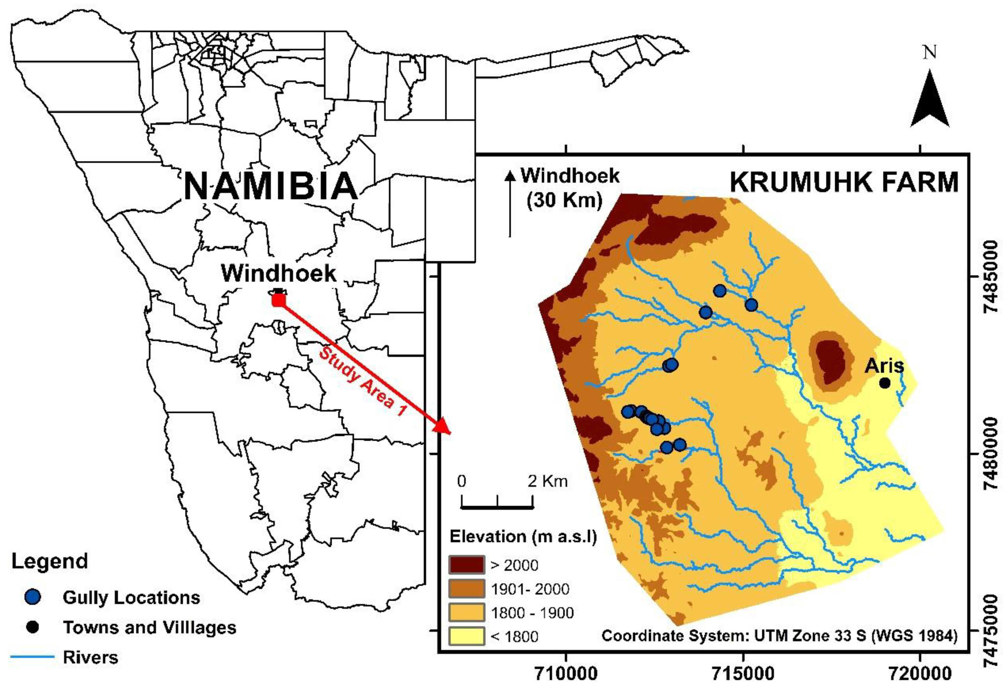
2. Study Site and Materials

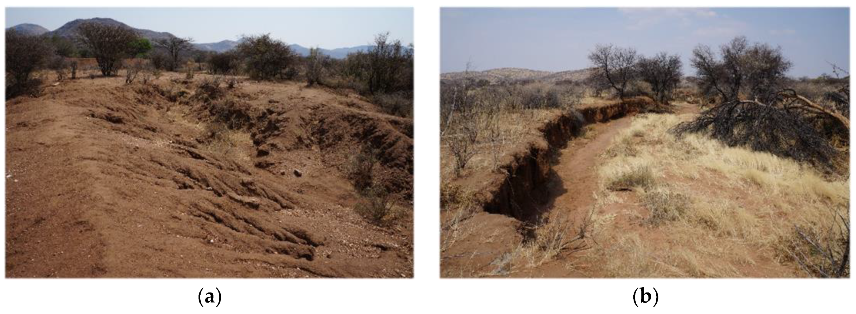
2.1. Study Site

Krumhuk Farm, located ca. 30 km south of Windhoek (Namibia), was selected for this study because it represents the typical central Namibia landscape (highlands in the central plateau) undergoing common land degradation problem of gullies. In addition, there is a historical research interest in the gully networks present in the farm [7,36] and restoration actions are currently being implemented in the area [12]. The locality map of Krumhuk, as well as the positions of main gullies identified in the farm to date are presented in Figure 1 [7,37].

Krumhuk Farm has an area of 8544 ha, a perimeter of 50.4 km and elevations ranging from 1753 m to 2335 m above sea level. With an average annual rainfall ranging from 250 mm to 350 mm, the predominant vegetation type is dense shrubland, with cattle ranching as the main farming practice. Dominant soils in the region are Eutric Leptosols and Lithic Leptosols [38], although in the study area a greater presence of Regosols has been observed, according to [39]. Both Leptosols and Regosols are common in eroding landscapes. The estimated average depth for the soils of the area is 1.84 m [39].

The farm is affected by at least nine individual gullies clearly differentiated. As reported by [7], the main triggering factors (knick points) derive from infrastructure (i.e., roads, fence lines) and the presence of domestic and wild animals. The erosion process is accelerated by the existence of an overgrazed soil that receives channeled surface runoff due to a topography composed of sandy flat valleys surrounded by steep slopes. Furthermore, many gullies develop lateral branches initiated from animal tracks. “Erosion headcuts progress upslope at all scales (micro to macro), cutting into adjacent intact soil surfaces” [7]. In addition to the direct damage that results from the soil loss, the drying of the surrounding landscapes and their sub-catchments, which were often the most productive, is of ecological significance. A detail report of the state of gullies in Krumhuk Farm can be found in [7].

2.2. TanDEM-X Data

The data used in this study are TanDEM-X (HRTI-3), acquired from a TerraSAR-X DLR mission for the generation of a DEM worldwide with high precision (according to the HRTI-3 standard) as the basis for scientific research and operational DEM commercial production [40]. The TanDEM-X specifications are shown in the

Table 1. TanDEM-X HRTI-3 (WGS 84 ellipsoid) data specifications [40].

Requirement	Definition	HRTI-3
Relative Vertical Accuracy	90% linear point-to-point error	2 m (slope < 20%)
Absolute Vertical Accuracy	90% linear error	10 m
Horizontal Accuracy	90% circular error	10 m
Spatial Resolution	Independent pixels	12 m

.

According to [41], the TanDEM-X relative vertical accuracy is sensitive to land cover type, typically yielding an RMSE of ±1.1 m for low vegetation areas (i.e., semi-desertified area in Krumuhk Farm). An important consideration is that, “although there are some exceptions in which SAR signal can penetrate the terrain surface (i.e., ice, snow or vegetation), in general, the TanDEM-X can be mostly regarded as a Digital Surface Model (DSM)”, hence artificial and natural structures such as households, groups of isolated rocks or dense vegetation could affect the terrain model [41].

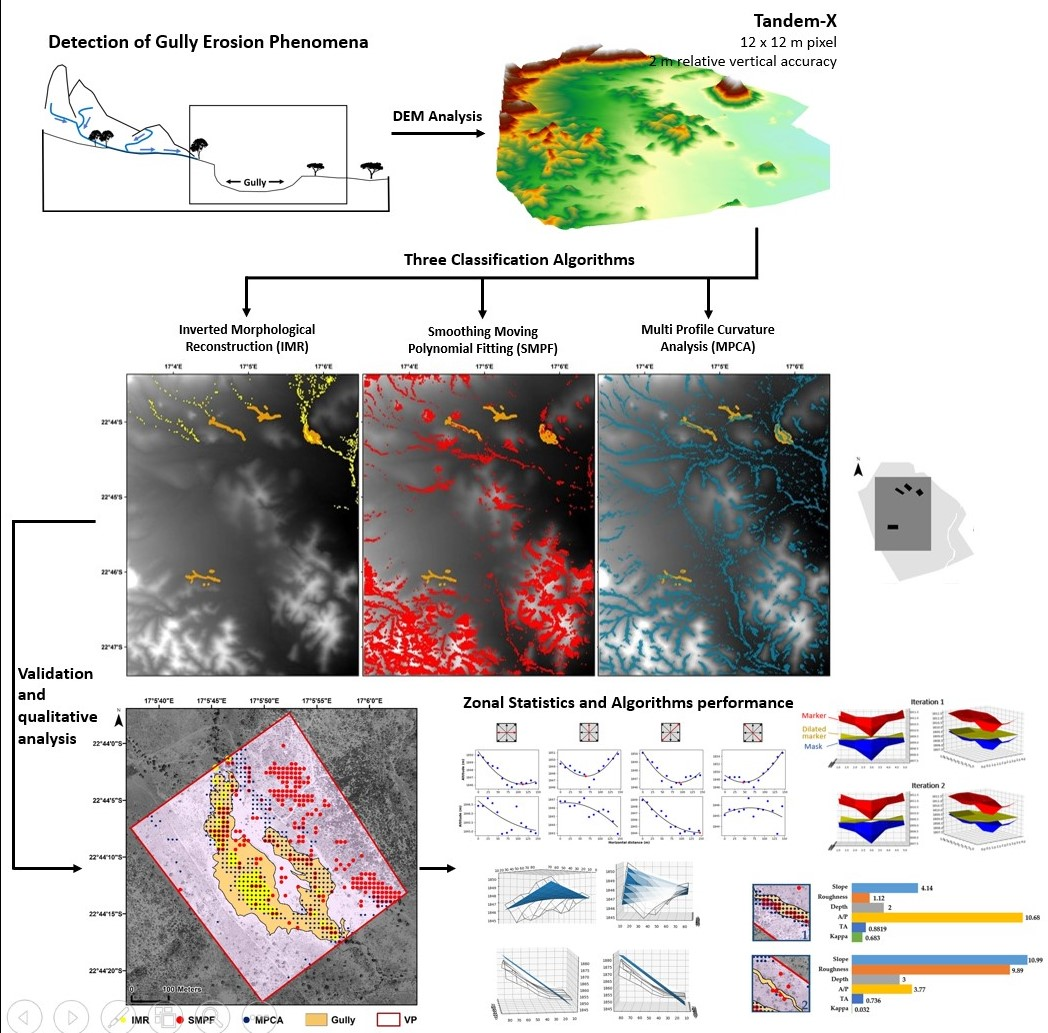
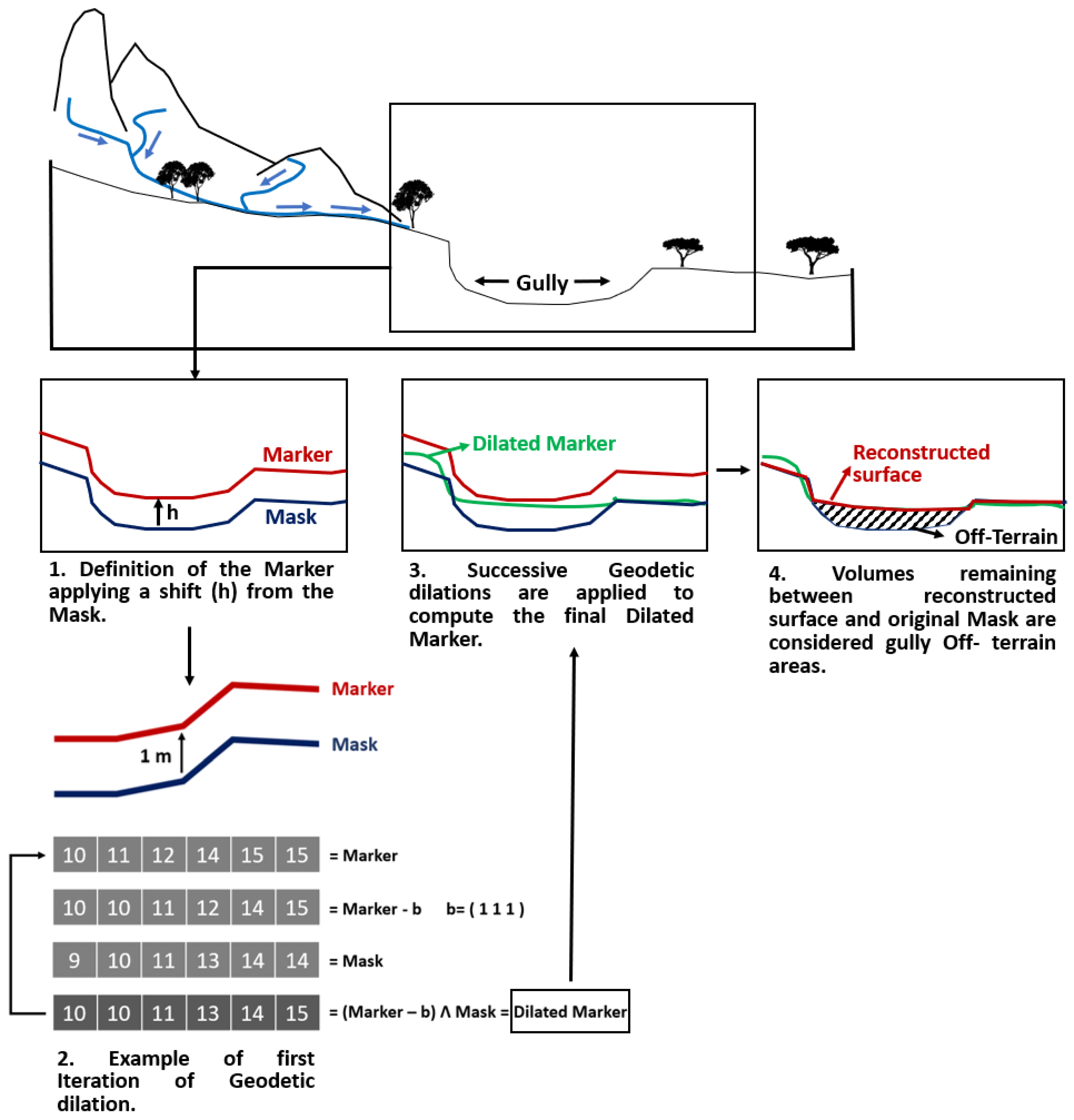
3. Methods for Gully Detection

3.1. Algorithms

Three algorithms are quantitatively and qualitatively evaluated to classify gully-affected areas using TanDEM-X data at the pixel level: Inverted Morphological Reconstruction (IMR), Smoothing Moving Polynomial Fitting (SMPF) and Multi-Profile Curvature Analysis (MPCA).

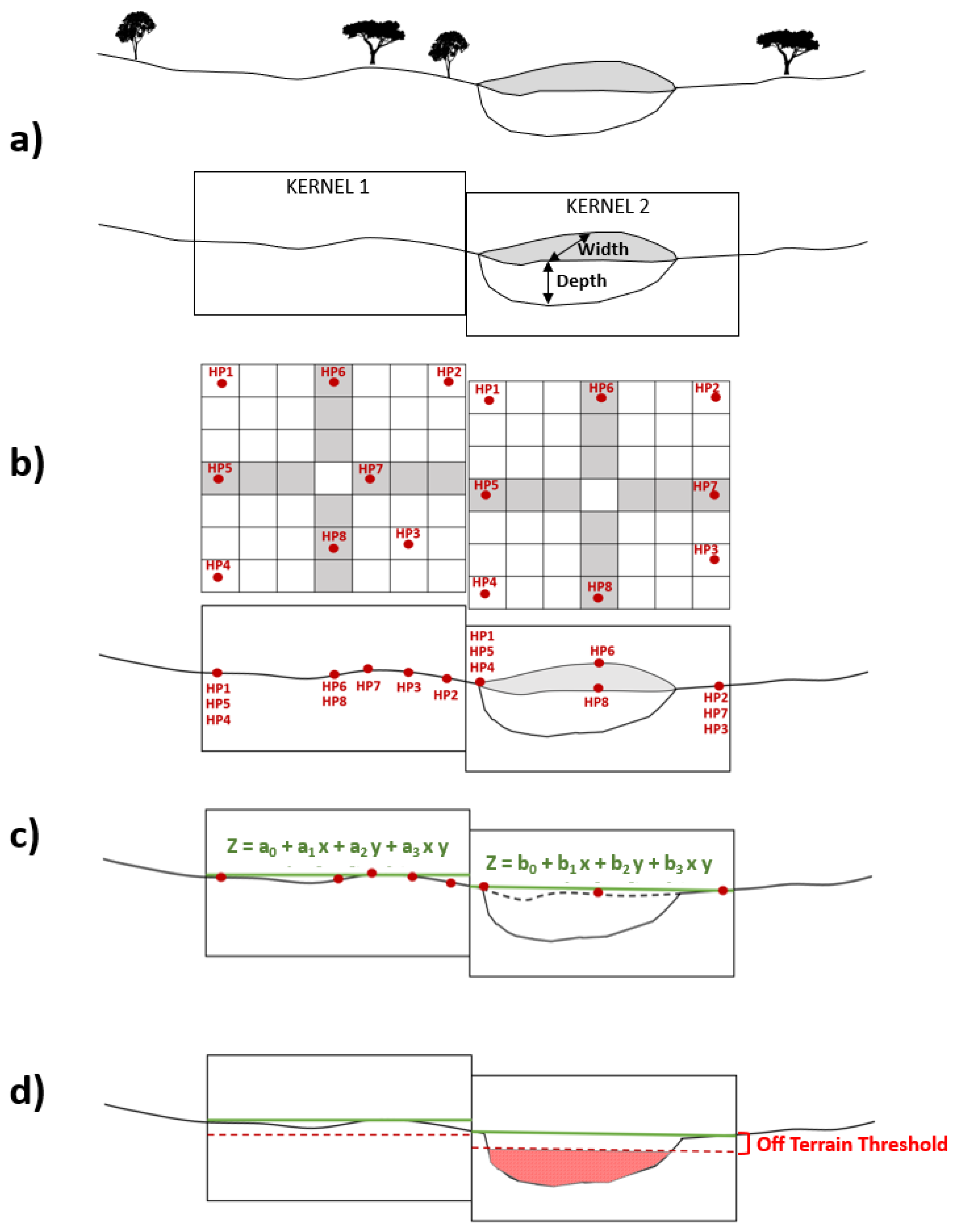
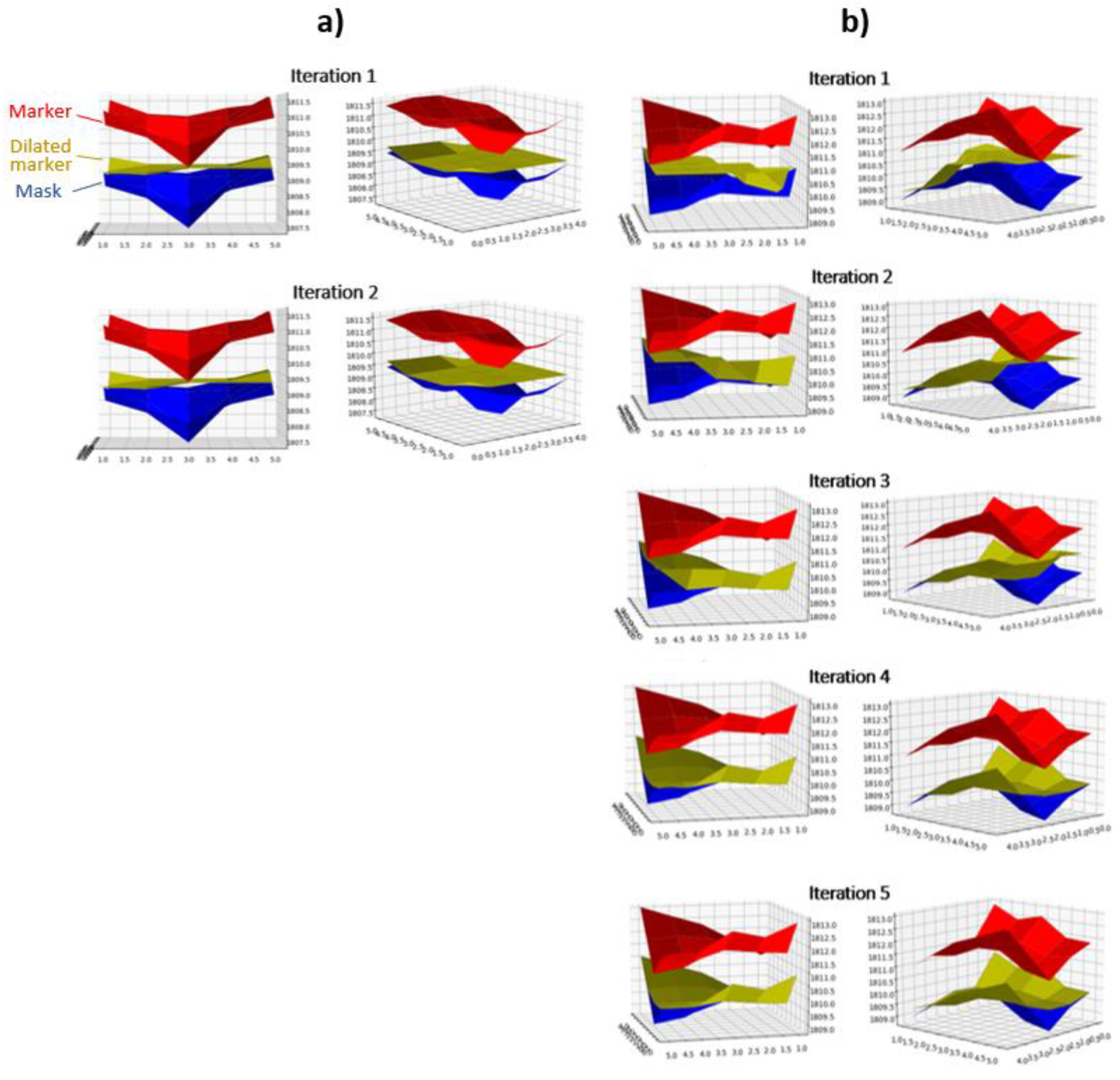
3.1.1. Inverted Morphological Reconstruction (IMR)

The Morphological Reconstruction (MR) method is based on morphology filtering and is widely applied in the field of image processing [42]. These methods were adapted by [43,44] to extract manmade structures as 3D off-terrain points above the ground surface from LiDAR point clouds. In our study, a modification of this algorithm for gully detection is developed. The algorithm is inverted to consider off-terrain elements as those areas below the surface of the natural terrain.

The MR requires two input images: mask and marker. The mask is the height profile represented by the original DEM, while the marker is a positive shifted copy of the mask considering a height (h) difference of the objects depth to be detected as specified in Equation (1).

marker = mask + h

(1)

A process of geodesic dilation is repeated until the dilated marker no longer changes. This is indicated in Equation (2), where b defines window size (simplified to one-dimension) and Λ is a pixel-based operation that takes the maximum value while comparing two raster images.

dilated marker = (marker − b) Λ mask

(2)

With e.g., b = (1 1 1) and Λ = pixel-wise max.

The definition of IMR is based on the fact that geodesic dilation [43,45] is applied to maintain the maximum pixel value when comparing the marker and the mask, thereby avoiding low off-terrain pixels. This constitutes a departure from classical MR applied by [43,44]. Figure 2 shows the theory behind the algorithm:

The height (h) and the window size (b) play a key role in the application of the algorithm since they will define the minimum detectable object on the surface in terms of depth and width.

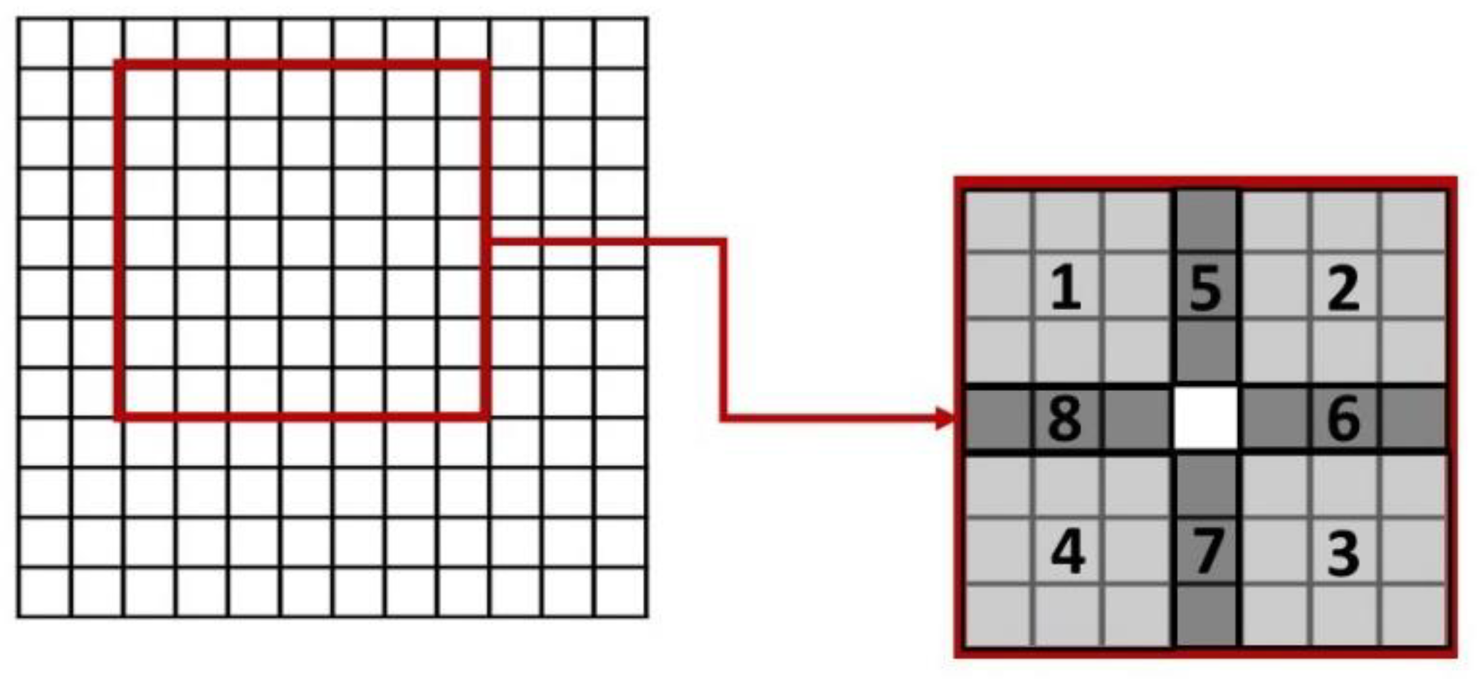
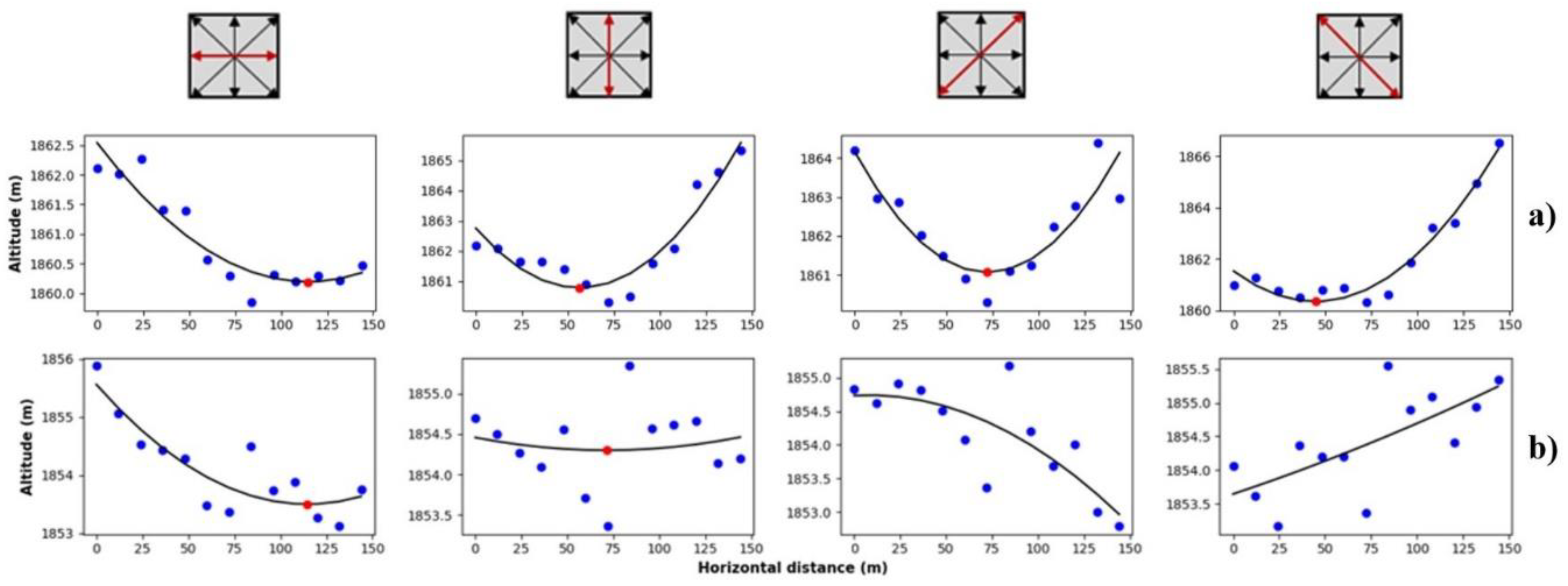
3.1.2. Smoothing Moving Polynomial Fitting (SMPF)

Polynomial Fitting is a generalized technique for the design of Digital Terrain Models (DTM) and Digital Surface Model (DSM) based on a discrete point dataset. Some examples of its application are [46,47].

If the discrete datasets exclude those points belonging to local depressions, such as gullies, this method can be adapted to generate a smooth DEM without the need to consider terrain gaps and other abrupt depressions at the gully-scale. To develop SMPF, a convolutional kernel with an odd number of columns and rows is designed and divided into eight zones (see Figure 3).

For each zone, the pixel containing the maximum height value is identified and eight points selected with an even distribution within the kernel (Figure 4b). This avoids points aggregation in a single zone. Using these high points (HP) as inputs, a local bilinear interpolation is carried out (Figure 4c) for each kernel, such that possible depressions in the terrain remain below the surface, defined by:

Z (x, y) = a₀ + a₁x + a₂y + a₃xy

(3)

The central pixel of the moving kernel within the original DEM is compared to the same pixel (in x-y coordinates) in the resulting surface to detect possible off-terrain pixels. As a final step, a threshold is applied to filter only those areas with a minimum height beneath the bilinear surface, and therefore potentially representing of being a gully (Figure 4d). Figure 4 illustrates the rationale of the developed algorithm in two-dimensions.

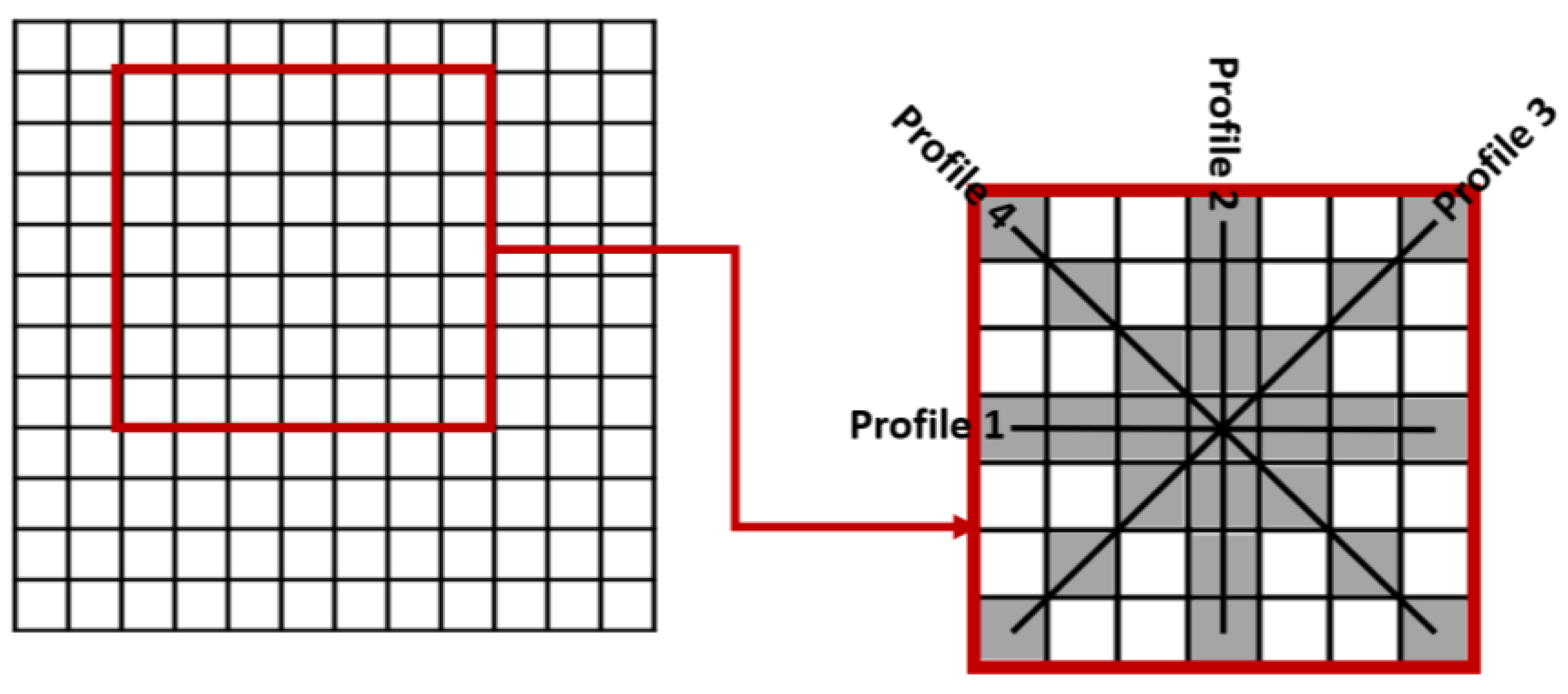
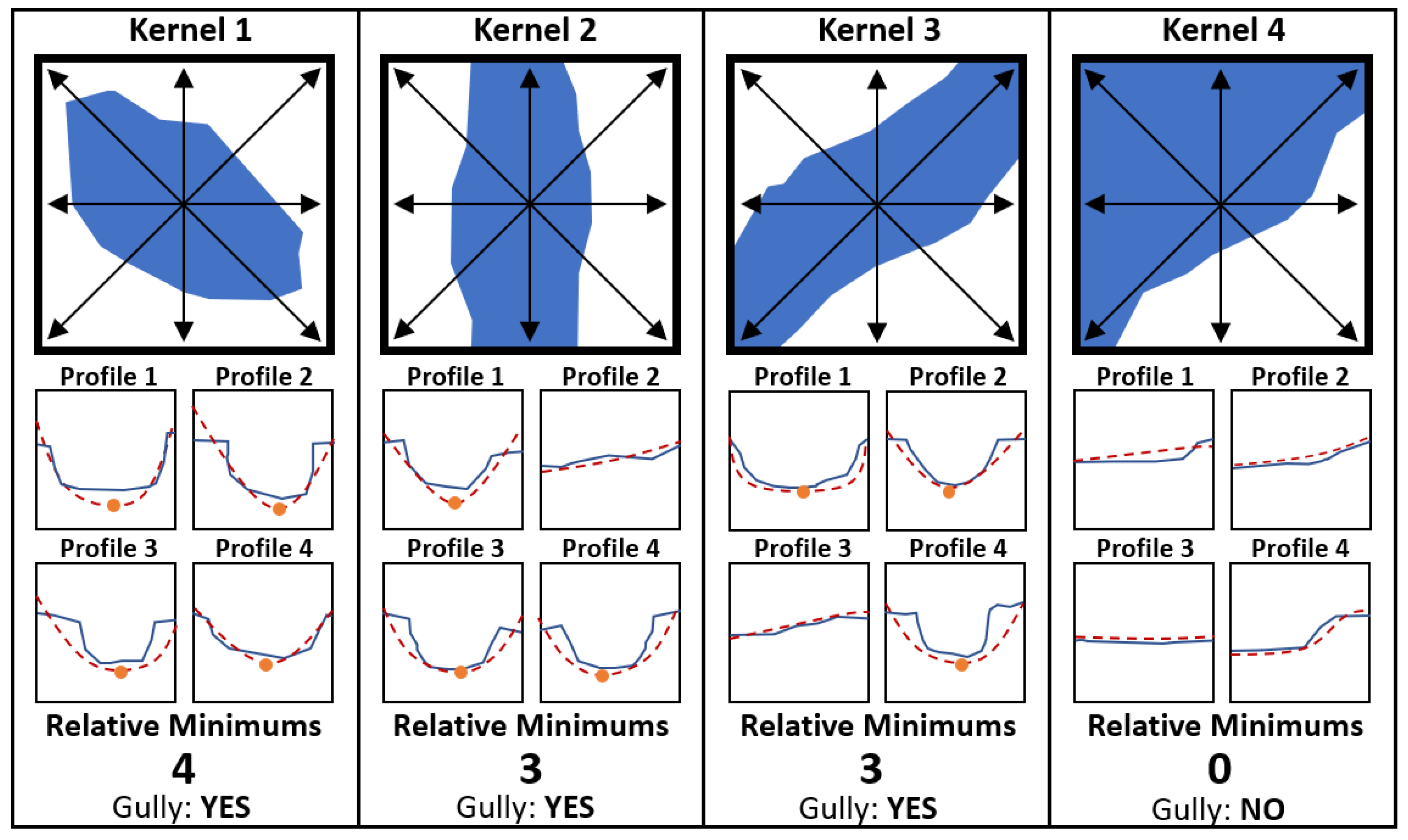
3.1.3. Multi-Profile Curvature Analysis (MPCA)

Characterization of micro-terrain features has been also explored to detect convex and concave features in the terrain [48]. The analysis of first and second derivatives of a function fitted to the terrain is a frequently used resource to describe terrain characteristics and to undertake GIS-based analysis for use in erosion models [49].

Infinitesimal calculus is applied in this approach for the detection of gullies, based on their morphology and profile curvature, under the assumption that a gully represents a Relative Minimum (RM) with convex form [50,51,52].

The algorithm is based on the analysis of the different profiles presented in a square kernel (with odd number of pixels), which is iterated over the full image. Four axes are drawn on this kernel (one vertical, one horizontal and two oblique) representing a row vector, a column vector and the two diagonal vectors of the kernel, respectively (see Figure 5).

Once these vectors are identified, a second-degree function (4) is adjusted to each.

Z(x) = a₀ + a₁x + a₂x²

(4)

According to the resultant functions, the first and second derivatives are calculated, and the condition stated in (5) is applied to define a favorable case of gully candidate for each profile:

$$\begin{array}{c}\mathrm{If}:\frac{dZ\left(XO\right)}{dx}=0\mathrm{AND}\frac{d^{2}Z\left(XO\right)}{d{x}^2}>0\to \mathrm{RM}=1\\ \mathrm{Else}:\mathrm{RM}=0\end{array}$$

(5)

If four or three functions (profiles) present an RM (first derivative equal to zero and second derivative positive), a gully is assumed to exist within the kernel. For fewer than three local minima in a kernel, it is assumed that there is no gully in this window.

The rationale of the algorithm is presented schematically in the Figure 6 through four hypothetical examples:

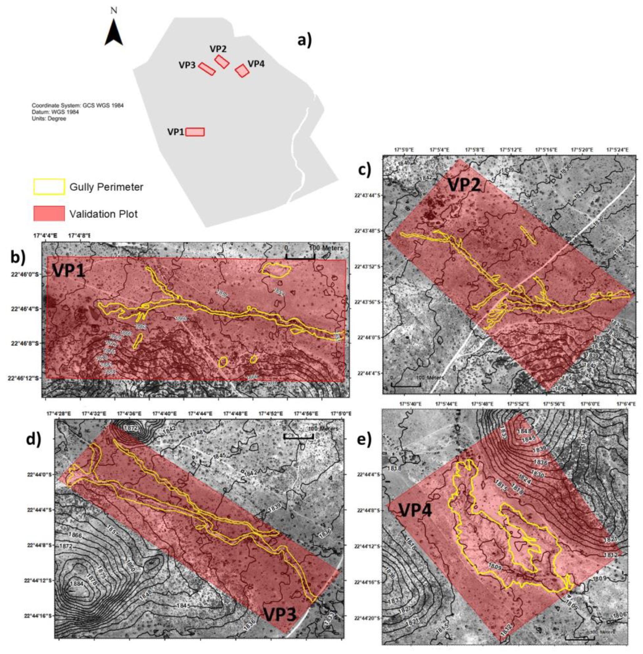
3.2. Field Gully Characterization

To evaluate the performance of the classification algorithms, reference data were collected directly in the field with Global Navigation Satellite System (GNSS) between June and August 2018. To reduce possible error sources derived from the temporal mismatch between ground truth and TanDEM-X production date (January 2015), the GNSS tracks were subsequently refined using high-resolution satellite imagery as a base map (Pleiades PHR Ortho 0.5 m spatial resolution, produced in November 2016).

An autonomous GPS receiver (Garmin GPS map 78s), with an accuracy <10 m and 95% confidence, was used. With the aim of observing the possible effects on algorithm performance, selection of the sub-study areas with the presence of gullies, namely Validation Plots (VP), was undertaken to maximize the diversity in gully typology (i.e., size, shape, activity). A summary of the four VPs and their corresponding gully attributes is presented in

Table 2. Summary description of the four Validation Plots (VPs) selected from Krumhuk Farm.

VP	VP Area (ha)	Gully Area (ha)	Gully Perimeter (km)	Gully Maximum Depth (m)	Gully Maximum Width (m)	Description
VP1	28.9	2.33	3.11	2	40	Main Gully #1 Secondary Gullies #4
VP2	42.4	1.92	3.77	4	30	Main Gully #1 Secondary Gullies #1
VP3	24.0	3.91	2.88	3	45	Main Gully #1 Secondary Gullies #1
VP4	29.9	6.60	2.66	6	150	Main Gully #1 Secondary Gullies #0

and shown graphically in Figure 7:

VP1 and VP2 enclose elongated gullies lengthwise, but differ in the lateral erosion activity (branching), which is presented in VP2 but not in VP1 (Figure 7). Conversely, VP3 contains two parallel V-shape gully channels that differ in their width and depth, but are both characterized by homogeneity in their cross section along the main gully axis. VP4 represents a large gully both in terms of width and depth, where its cross section is predominantly U-shaped, as defined in [52].

3.3. Algorithm Settings

A critical aspect for attaining the best classification results is the configuration of the algorithms settings. IMR is influenced by two parameters: Kernel size and mask shift. Kernel size controls the width of the minimum detectable object, and the mask shift the minimum height of the object. Since most of the gullies that exist in Krumhuk range from 15–100 m width and 1–4 m depth, parameters ranging within these intervals were tested. For SMPF, the same criteria were used to select the size of the kernel and off-terrain threshold. MPCA is controlled only through the kernel size but the shape of the surrounding terrain needs to be captured, therefore this parameter was also explored for large dimensions (up to 180 m).

Different combinations for the algorithm parameters were tested and summarized for the four VPs presented in Section 3.2 (

Table 3. Results of the three algorithms tested with different configuration settings. The following parameters are evaluated and compared: Kernel Size (KS), Mask Shift (MS), Off-Terrain Threshold (OT), Producer Accuracy (PA), User Accuracy (UA), Cohen Kappa (KAPPA) and TA (Total Accuracy).

IMR
KS (m)	OT (m)	PA (Gully)	PA (Non-Gully)	UA (Gully)	UA (Non-Gully)	KAPPA	TA
36	1	0.439	0.672	0.142	0.906	0.058	0.646
60	1	0.035	0.999	0.895	0.893	0.060	0.893
84	1	0.022	1.000	1.000	0.892	0.038	0.892
108	1	0.009	1.000	1.000	0.890	0.017	0.891
36	2	0.661	0.596	0.169	0.934	0.113	0.603
60	2	0.071	0.999	0.944	0.896	0.118	0.897
84	2	0.028	1.000	1.000	0.892	0.049	0.893
108	2	0.009	1.000	1.000	0.890	0.017	0.891
36	4	0.837	0.505	0.173	0.961	0.128	0.541
60	4	0.071	0.999	0.944	0.896	0.118	0.897
84	4	0.028	1.000	1.000	0.892	0.049	0.893
108	4	0.009	1.000	1.000	0.890	0.017	0.891
SMPF
KS (m)	MS (m)	PA (Gully)	PA (Non-Gully)	UA (Gully)	UA (Non-Gully)	KAPPA	TA
60	1	0.255	0.843	0.168	0.901	0.081	0.778
84	1	0.323	0.830	0.191	0.908	0.119	0.775
108	1	0.332	0.747	0.140	0.900	0.050	0.701
132	1	0.333	0.659	0.108	0.888	−0.004	0.623
84	1.5	0.134	0.948	0.242	0.898	0.102	0.858
60	2	0.019	0.986	0.142	0.890	0.008	0.879
84	2	0.041	0.981	0.218	0.892	0.035	0.878
108	2	0.068	0.952	0.149	0.892	0.026	0.854
132	2	0.078	0.903	0.091	0.888	−0.020	0.812
60	3	0.000	0.997	0.000	0.889	−0.005	0.887
84	3	0.002	0.996	0.056	0.889	−0.004	0.886
108	3	0.010	0.988	0.101	0.889	−0.002	0.880
132	3	0.022	0.959	0.062	0.888	−0.026	0.856
MPCA
KS (m)		PA (Gully)	PA (Non-Gully)	UA (Gully)	UA (Non-Gully)	KAPPA	TA
36		0.337	0.751	0.144	0.901	0.055	0.705
60		0.400	0.819	0.215	0.917	0.158	0.773
84		0.452	0.851	0.273	0.926	0.235	0.807
108		0.506	0.865	0.317	0.934	0.294	0.825
132		0.554	0.866	0.338	0.940	0.328	0.831
156		0.581	0.861	0.341	0.943	0.338	0.830
180		0.000	1.000	0.000	0.890	0.000	0.890

According to the results obtained for each algorithm configuration, the following parameters (see Table 4) were selected prior to a more exhaustive analysis and interpretation, both at the qualitative and quantitative levels.

).

4. Results

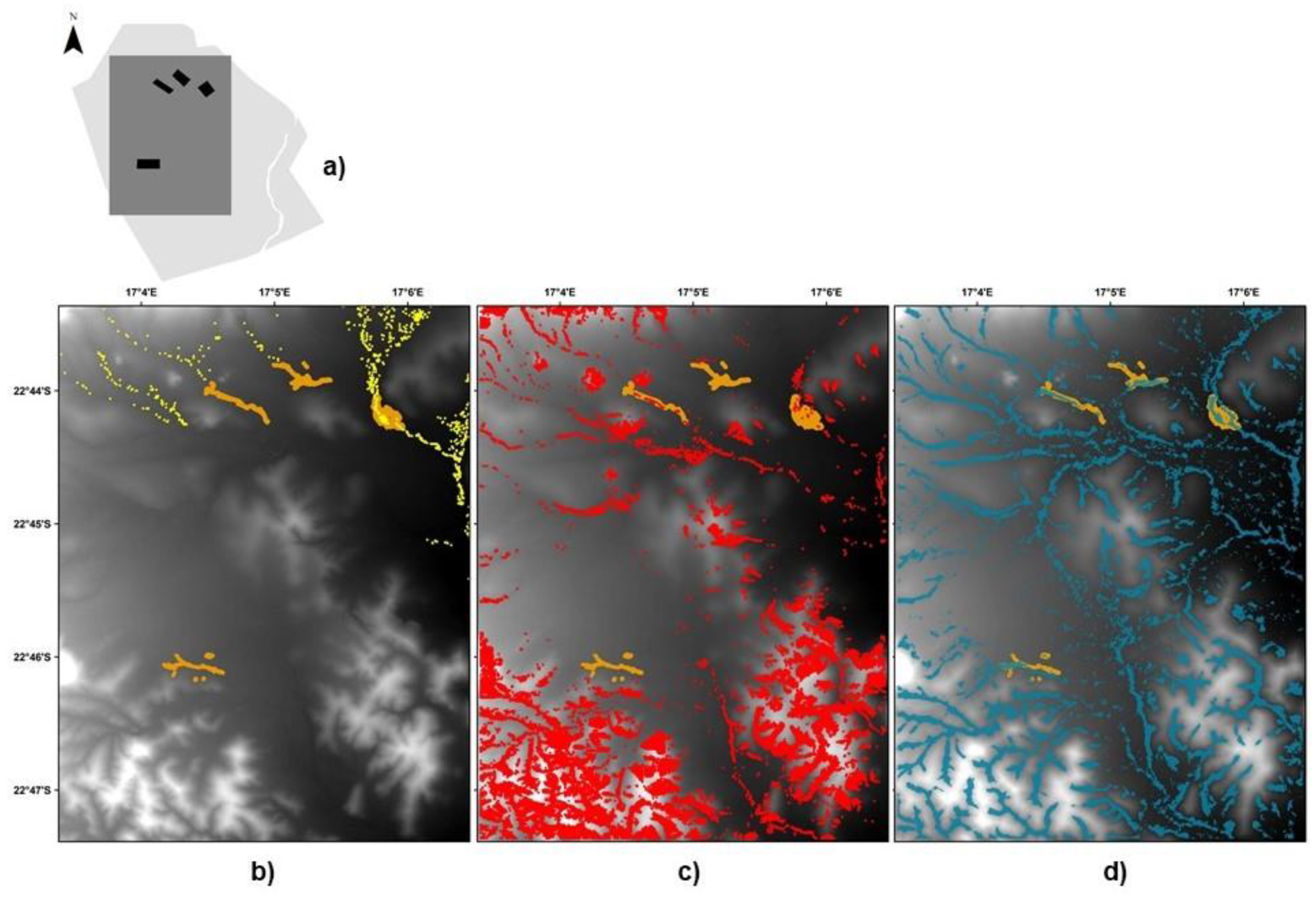
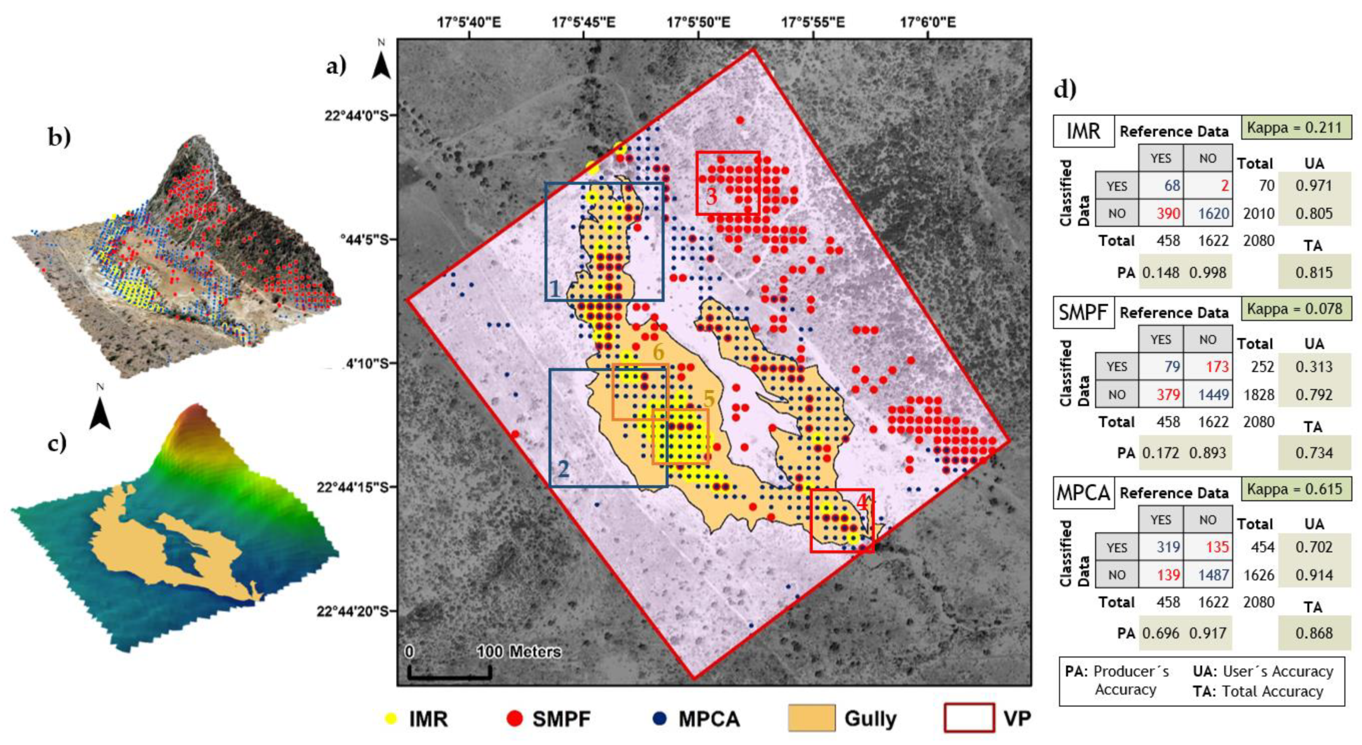
4.1. Visual Interpretation of Results

Figure 8b–d shows the results generated by the three proposed methods (IMR, SMPF and MPCA). These results are derived from the algorithms configurations detailed in

Table 4. Final selection of algorithm settings.

	IMR	SMPF	MPCA
Kernel Size	60 × 60 m	84 × 84 m	156 × 156 m
Mask Shift	2 m	-	-
Off-Terrain Threshold	-	1.5 m	-

and applied to the processed extent, named Area of Interest (AOI) and clipped from TanDEM-X in Krumhuk Farm.

Figure 8b shows that IMR detects gullies only in the northern region of our AOI, depicting shapes of elongated form. In this approach, it is evident that fewer points are classified as potential gullies compared to the other methods. This could be due to sensitivity and parameter settings of the algorithm (i.e., depth of gullies, mask, and window size), implying that the method could be suitable to detect big gullies as opposed to smaller ones.

In Figure 8c, potential gullies are detected using SMPF. Through this technique concentrated points of potential gullies (in red) were distinguished in the southern part of our AOI that are also nearby elevated regions (hilly/mountainous area). In addition, typical linear gully structures can be identified from visual interpretation [33] in the northern parts.

The MPCA method detects what appear to be potential gullies (in blue) throughout the area of interest (Figure 8d), creating dendritic and linear forms that are characterized by as good indicators of gully network morphology [33]. The gullies that are identified are more evenly distributed throughout the AOI. However, MPCA is less influenced by hilly topography than SMPF, as observed in the southern parts of the AOI.

4.2. Validation and Analysis of Results

For each VP, accuracy assessment of the three algorithms is undertaken quantitatively and presented in the form of Confusion Matrices [53]. Qualitative analysis is also performed, paying special attention to those singular areas where the gully morphology and other topographic factors (i.e., slope, topographic roughness) can substantially affect the performance of the algorithms. Result summaries are presented below for the VP1 and VP4. These two VPs are of particular interest, given that they present the poorest (VP1) and the best (VP4) results among the four validation areas, respectively. In addition, interesting and/or distinct scenarios are captured, and extensive qualitative analysis can also be conducted and extrapolated for VP2 and VP3.

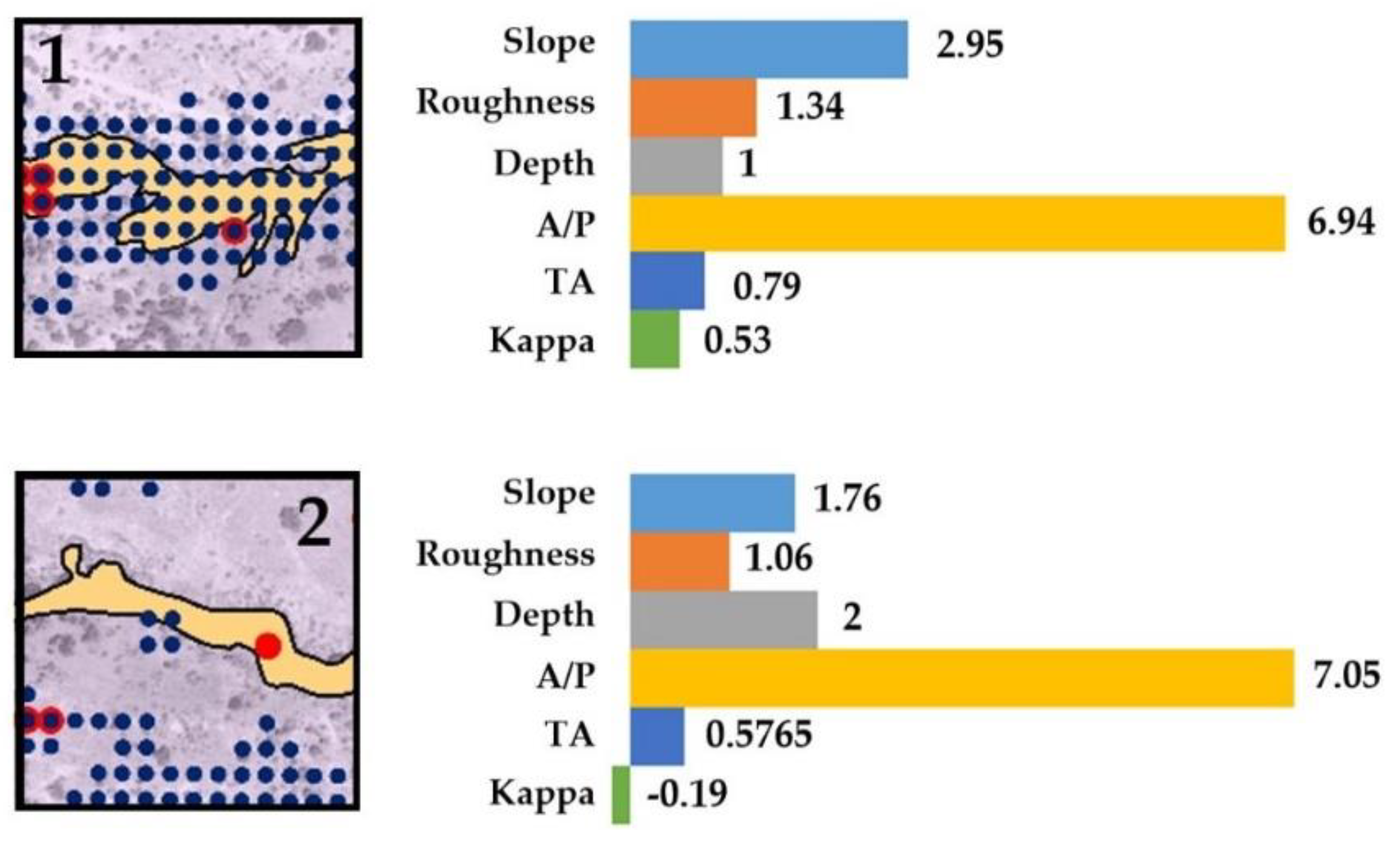
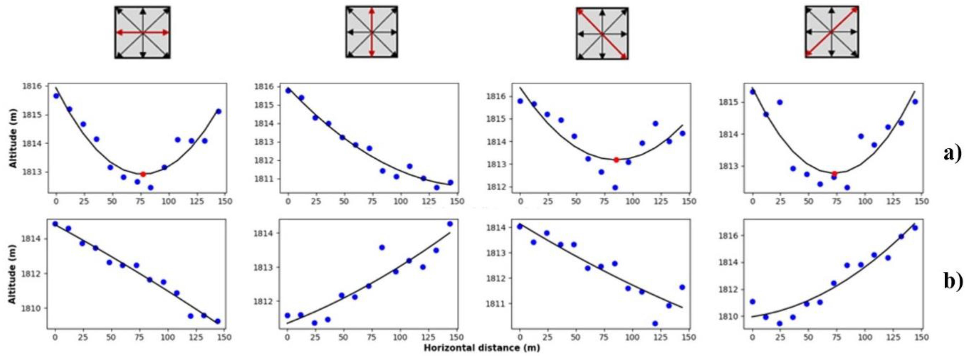
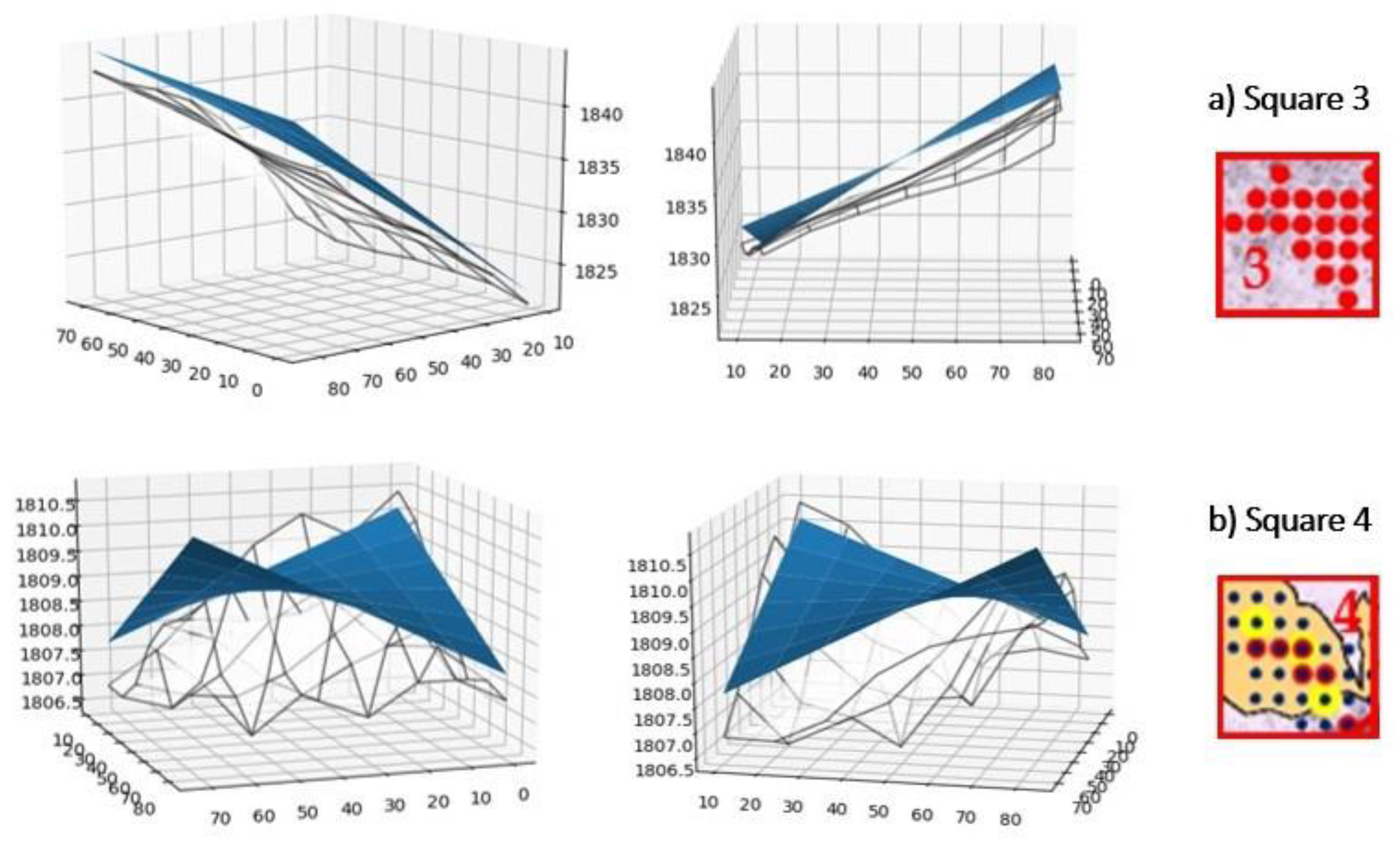
4.2.1. Validation Plot 1 (VP1)

Figure 9a shows that gullies inside VP1 are partially detected by MPCA, but the performance differs significantly from west to east over the gully network. From a zonal analysis, it is noticed that in the western part (enclosed by Square 1), where the gully is wider (up to 30–35 m), results achieve approximately TA of 0.80 with 0.5 Kappa value. Nevertheless, the gully sections (15–20 m width) located in the eastern part (Square 2) are classified by MPCA deficiently (TA 0.57 and Kappa −0.19). An analysis comparing zones enclosed by Squares 1 and 2 shows that, in this case, there is no strong correlation between topographic factors (slope, topographic roughness) and the quality of MPCA results. In addition, the Area-Perimeter (A/P) ratio and gully depth are not significant parameters in this case (see Figure 10).

In this case, the gully shape and its surroundings’ topography play an important role in the classification due to minor gully dimensions. Square 1 encloses a V-gully shape section with smooth side-wall slopes and surrounded by gentle hillsides (see Figure 11a), providing a general convex shape within the MPCA kernel (156 m side). On the other hand, Square 2 encloses a U-shape gully section surrounded by plain topography (see Figure 11b).

Focusing in the eastern parts of the main gully (Square 3), an unpredicted performance of the MPCA detection method is also observed given that there is substantial error of omission for the gully class. However, the algorithm detects pixels shifted 20–30 m in the south, resulting in error of commission. Sub-areas are selected (Square 3 and Square 4) to verify how the algorithm is producing the results. Figure 12a shows that a terrain micro-depression (<2 m deep) is detected within Square 4, which can be also motivated by the presence of off-terrain structures such as trees or piles of rocks.

With this in mind, natural or man-made objects appear to distort the adjustment causing classification errors. In this case (Square 3), the gully channel is surrounded by a group of trees, increasing the elevation of the terrain within a specific pixel. This effect, combined with the limited dimensions of the gully channel, generates the false shape of concavity in the function adjusted to the terrain (Figure 12b). This phenomenon of distorting off-terrain objects above the DEM surface, considered as a possible source of errors, should be addressed setting quality threshold in the robustness of the fitting to reduce the amount of isolated scattered points classified as gullies.

Secondary gullies are also detected using the MPCA, which are characterized by their small depth (<0.5 m), with the implication that depth holds a lower influence over gully identification with MPCA than width.

While IMR fails to any pixels in this VP (both inside and outside the gully extent), SMPF presents very poor performance, and those pixels classified as gullies are in a sloped surface, as introduced in Section 4.1 (visual interpretation of results).

Examination of the confusion matrix confirms that the most reliable method is MPCA, with a Total Accuracy (TA) of 0.80 and Kappa Value of 0.112, the highest of the three, considering the whole area of the VP1. Although IMR and SMPF present little or no commission errors, their omission error falls beneath acceptable levels (UA and PA < 0.15) for the gully class, which is also reflected by their random Kappa values.

4.2.2. Validation Plot 4 (VP4)

The statistics for VP4, enclosing the gully with the largest dimensions among those measured, presents an improvement in the performance for MPCA and specially IMR methods, as shown in the Figure 13. IMR classifies almost all pixels correctly as gullies achieving a UA of 0.97. SMPF presents also an improvement for gully class UA, nevertheless the failure rate is again high in areas where topography changes from flat to slope.

MPCA appears well-suited to gully detection (0.696 PA and 0.702 UA), with a low failure rate for non-gully areas (0.917 PA and 0.914 UA). Nevertheless, differences arise as a function of the area considered. The zonal analysis was therefore repeated for two areas where a large difference in the results is observed, highlighting the influence of kernel size upon derived gully dimensions. Comparing two gully sections with similar depths, the MPCA classification yields a near perfect accuracy when its width is captured entirely by the convolutional kernel (Figure 14a). However, for those areas where the kernel partially captures the gully along ones of its edges, the result is unsatisfactory (Figure 14b). This reinforces the observation, described for VP1 under Section 4.2.1, that width is a major factor to consider when detecting gullies. While the shape of the deepest parts of the gully has been perfectly outlined, regions close to the edges fail to be classified, possibly due to the difficulty in defining the precise perimeter of the gully when gully walls are not vertical (instead presenting a gentle slope). This omission error in gully class can also be justified by the fact that the gully width is larger than the kernel side, such that its cross section is not captured within the kernel (Figure 14b). This leads to the misclassification of the gully as a normal slope. An adaptive kernel that measures the robustness of the adjustment is therefore necessary to improve MPCA.

Comparing again different scenarios for SMPF, it is clear that hillsides zones represent a source of error. Nonetheless, when the gully size is well-defined with vertical walls and the kernel size captures the gully outside borders, the algorithm succeeds in the gully detection (see Figure 15).

Analyzing the results for IMR, we can observe two different situations. Figure 16 shows a case where a gully is detected once the dilated marker (yellow) remains stable and above the mask (blue) (Square 5 in Figure 13). A second study case is presented to describe the process when a dilated marker adopts the shape and height of the mask after five iterations. The final position of the dilated marker is too close to the mask, such that the central pixel is not identified as a gully (Square 6 in Figure 13).

The results are, nevertheless, satisfactory for MPCA, with a TA of 0.868 and an improved Kappa of 0.615. IMR presents an 0.998 accuracy for PA in non-gully areas, and in this case also 0.971 for UA in gully class. SMPF again produces low percentage scores for gully class, both in PA (0.172) and UA (0.313). IMR and SMPF have in this case lower TA (0.815 and 0.792) and Kappa (0.211 and 0.078) than MPCA.

5. Discussion

The classification of gully-affected within TanDEM-X data provides promising results, considering that the developed methods are fully automated and can be applied over large areas. The three algorithms proposed here are in an initial stage of development and there is still a room for improvement, both for each method individually and in a combined approach.

Based on quantitative validation results (Table 3), MPCA obtains an overall accuracy (TA) of 0.829, Kappa of 0.337, UA of 0.341 (Gully) and 0.942 (non-Gully), and PA of 0.580 (Gully) and 0.860 (non-Gully). Nevertheless, these numbers can achieve accuracies close to 0.90 and Kappa values above 0.50 when the dimensions of the gullies are larger than 35–40 m in width. Conversely, off-terrain elements (i.e., groups of trees or rocks) act as outliers in the DEM, negatively affecting the MPCA while fitting the second order polynomial to the actual gully shape. Large gullies, the width of which exceed the kernel size, will only be identified in their center, with zones close to the gully edge misclassified. Another limitation of MPCA is its inability to discriminate endorheic depressions with similar gully dimensions. Further studies should therefore adopt change detection techniques to capture the dynamic nature of the gullies.

In order to increase the efficacy of MPCA, an improved version should consider an adaptive kernel size that includes robust fitting methods (i.e., RANSAC) for the adjustment. This robust fitting approach could be also implemented in order to reduce the amount of isolated scattered points classified as gullies.

IMR and SMPF are inapplicable for practical purposes at this stage of development; nevertheless, some useful learnings have arisen. The application of IMR has demonstrated its reliability in detecting large gullies (error of omission for non-gully class is almost null), although realistic gully outlines cannot be directly derived. Its main drawback, however, is the limited identification of pixels as gullies and, consequently, the overall error of omission for the gullies class is high (>0.90). Conversely, SMPF exhibits a high sensitivity to variable gully sizes and irregular topography, resulting in frequent over-classification of gullies in areas with steep slopes. Filtering of hillsides and the implementation of an adaptive kernel size could improve reliability for plane terrains.

Benchmarking relative to other studies is complex, given the disparity in study areas, and hence gully type, and sensors. Despite this, MPCA results are comparable [32,34], and in some cases superior [33], to previous attempts to classify gullies from remotely sensed products. For instance, the accuracy of the results achieved with MPCA are moderately higher than those from [32]. With a higher spatial resolution (SPOT 9 with 10 m compared to TanDEM-X 12 m) this study achieved 0.76 overall accuracy (against 0.83 of MPCA), although the total Kappa was slightly superior (0.52 against our 0.35). The total accuracy achieved by [34] was 0.62, lower than MPCA despite using higher resolution imagery (Quickbird, 0.6 m). Assuming that the MPCA results are scalable to higher spatial resolutions, the MPCA would obtain better results than [34] both for the TA and omission/commission errors if they are implemented on high-resolution DEMs.

As anticipated, the main limitation of the methods tested and documented in this article is the underestimation of gullies smaller than TanDEM-X’s areal resolution and relative vertical accuracy. This led to the general misclassification of gullies sections with less than 2 m depth or 12 m width.

6. Conclusions

The need for large area gully monitoring and mapping in Namibia is becoming crucial for the planning of regional strategies to tackle land degradation and for providing raw data for exhaustive research in geomorphology processes. The methods developed here provide a foundation for the development of more reliable, fully automatic standardized techniques to detect gully presence and to prioritize efforts in their prevention and remediation. After comparing the three algorithms (IMR, SMPF and MPCA), it is evident that MPCA yields the best results and should be prioritized for further development. The fusion of MPCA with IMR and SMPF based on tree decision algorithms according to the terrain and gully characteristics also require exploration. Three main actions are suggested:

(1)

improve MPCA according to the suggestions provided in the discussion to achieve at least 0.50 in gully class both of UA and PA.

(2)

derive geomorphological and geomorphometric features from the pixel-based classification, such as gully outline and depth, in order to estimate gully volumes.

(3)

explore the fusion of TanDEM-X data with multispectral (i.e., Sentinel 2) and RADAR (i.e., Sentinel 1), to perform time series analysis and monitor gully evolution and its erosion activity. This can generate valuable knowledge of gully dynamics for geomorphologists and agronomists working on land degradation in Namibia. In this way, gully categorization can also be implemented as part of the automatic gully identification method; for example, in classifying their activity as low, medium, or high and estimating the economic damage for commercial and communal farmers.

The presented approach contributes to gully erosion mapping for large areas (i.e., Namibia) and sets the foundation for further analysis focused on two potential applications: (1) the development of a national gully database in Namibia based on remote sensing and DEM analysis; and, (2) the generation of solutions to monitor the evolution of the geomorphological characteristics of individual gully networks at the individual farm scale, using multispectral remote sensing products (i.e., Sentinel 2) in combination with polarimetry and interferometry (i.e., DInSAR) RADAR techniques and products (i.e., Sentinel 1). This second approach is of particular interest given that gullies are dynamic phenomena and studies focused on the monitoring of gully sedimentation flows remain infrequent [54].

References

1. Valentin, C.; Poesen, J.; Li, Y. Gully erosion: Impacts, factors and control. Catena 2005, 63, 132–153. [Google Scholar] [CrossRef]
2. Fao Soils Portal: Soil Degradation. Available online: http://www.fao.org/soils-portal/soil-degradation-restoration/en/ (accessed on 29 September 2018).
3. Republic of Namibia, Ministry of Environment and Tourism. Third National Action Programme for Namibia To Implement the United Nations Convention to Combat Desertification 2014–2024; Republic of Namibia, Ministry of Environment and Tourism: Windhoek, Namibia, 2014; p. 80.
4. Wasson, R.J.; Caitcheon, G.; Murray, A.S.; McCulloch, M.; Quade, J. Sourcing sediment using multiple tracers in the catchment of Lake Argyle, Northwestern Australia. Environ. Manag. 2002, 29, 634–646. [Google Scholar] [CrossRef]
5. Krause, J.S.; Franks, A.K.; Kalma, S.W.; Loughran, J.D.; Rowan, R.J. Multi parameter fingerprinting of sediment deposition in a small gullied catchment in SE Australia. Catena 2003, 53, 327–348. [Google Scholar] [CrossRef]
6. Huon, S.; Bellanger, B.; Bonté, P.; Sogon, S.; Podwojewski, P.; Girardin, C.; Valentin, C.; de Rouw, A.; Velasquez, F.; Bricquet, J.-P.; et al. Monitoring soil organic carbon erosion with isotopic tracers: Two case studies on cultivated tropical catchments with steep slopes (Laos, Venezuela). In Soil Erosion and Carbon Dynamics, 1st ed.; Roose, E.J., Lal, R., Feller, C., Barthés, B., Stewart, B., Eds.; Taylor & Francis: Boca Raton, FL, USA, 2006; pp. 301–328. [Google Scholar]
7. Pringle, H.; Zimmermann, I.; Tinley, K. Accelerating landscape incision and the downward spiralling rain use efficiency of Namibian rangelands. Agricola 2011, 21, 43–52. [Google Scholar]
8. Poesen, J.; Vandaele, K.; van Wesemael, B. Gully erosion: Importance and model implications. In Modelling Soil Erosion by Water; Springer: Berlin/Heidelberg, Germany, 1998; Volume 55, pp. 285–311. [Google Scholar] [CrossRef]
9. Poesen, J. Soil erosion in the Anthropocene: Research needs. Earth Surf. Process. Landf. 2018, 43, 64–84. [Google Scholar] [CrossRef]
10. Sean, B.J.; Wells, R.R. Gully erosion processes, disciplinary fragmentation, and technological innovation. Earth Surf. Process. Landf. 2019, 44, 46–53. [Google Scholar] [CrossRef]
11. Castillo, C.; Perez, R. Comparing the Accuracy of Several Field Methods for Measuring Gully Erosion. Soil Sci. Soc. Am. J. 2012, 76, 1319–1332. [Google Scholar] [CrossRef] [Green Version]
12. SASSCAL Research Portfolio: Task 041: Landscape Literacy. Available online: http://sasscal.org/wp-content/uploads/external-assets/tasksheets/task_041_na_ag.pdf (accessed on 15 July 2017).
13. Burkard, M.B.; Kostaschuk, R.A. Initiation and evolution of gullies along the shoreline of Lake Huron. Geomorphology 1995, 14, 211–219. [Google Scholar] [CrossRef]
14. Betts, H.D.; DeRose, R.C. Digital elevation models as a tool for monitoring and measuring gully erosion. Int. J. Appl. Earth Obs. Geoinf. 1999, 1, 91–101. [Google Scholar] [CrossRef]
15. Martínez-Casasnovas, J.A.; Ramos, M.C.; Poesen, J. Assessment of sidewall erosion in large gullies using multi-temporal DEMs and logistic regression analysis. Geomorphology 2004, 58, 305–321. [Google Scholar] [CrossRef]
16. Ionita, I. Gully development in the Moldavian Plateau of Romania. Catena 2006, 68, 133–140. [Google Scholar] [CrossRef]
17. James, L.A.; Watson, D.G.; Hansen, W.F. Using LiDAR data to map gullies and headwater streams under forest canopy: South Carolina, USA. Catena 2007, 71, 132–144. [Google Scholar] [CrossRef]
18. Collins, B.D.; Brown, K.M.; Fairley, H.C. Evaluation of Terrestrial LIDAR for Monitoring Geomorphic Change at Archeological Sites in Grand Canyon National Park; USGS Publications Warehouse: Reston, VA, USA, 2008. [CrossRef]
19. Evans, M.; Lindsay, J. High resolution quantification of gully erosion in upland peatlands at the landscape scale. Earth Surf. Process. Landf. 2010, 35, 876–886. [Google Scholar] [CrossRef]
20. Stöcker, C.; Eltner, A.; Karrasch, P. Measuring gullies by synergetic application of UAV and close range photogrammetry—A case study from Andalusia, Spain. Catena 2015, 132, 1–11. [Google Scholar] [CrossRef]
21. Höfle, B.; Griesbaum, L.; Forbriger, M. GIS-Based detection of gullies in terrestrial lidar data of the cerro llamoca peatland (Peru). Remote Sens. 2013, 5, 5851–5870. [Google Scholar] [CrossRef]
22. Gómez-gutiérrez, A.; Schnabel, S.; Berenguer-sempere, F.; Lavado-contador, F.; Rubio-delgado, J. Using 3D photo-reconstruction methods to estimate gully headcut erosion. Catena 2014, 120, 91–101. [Google Scholar] [CrossRef]
23. Castillo, C.; Marin-Moreno, V.J.; Pérez, R.; Munoz-Salinas, R.; Taguas, E.V. Accurate automated assessment of gully cross-section geometry using the photogrammetric interface FreeXSapp. Earth Surf. Process. Landf. 2018, 43, 1726–1736. [Google Scholar] [CrossRef]
24. Morgan, R.P.C. Soil Erosion and Conservation, 3rd ed.; Blackwell Science Ltd.: Malden, MA, USA, 2013; pp. 65–66. [Google Scholar]
25. Billi, P.; Dramis, F. Geomorphological Investigation on Gully Erosion in the Rift Valley and the Northern Highlands of Ethiopia. Catena 2003, 50, 353–368. [Google Scholar] [CrossRef]
26. Vandekerckhove, L.J.; Poesen, J.; Govers, G. MidTerm Gully Headcut Retreat Rates in Southeast Spain Determined from Aerial Photographs and Ground Measurements. Catena 2003, 50, 329–352. [Google Scholar] [CrossRef]
27. Marzolff, I.; Poesen, J. The potential of 3D gully monitoring with GIS using high-resolution aerial photography and a digital photogrammetry system. Geomorphology 2009, 111, 48–60. [Google Scholar] [CrossRef]
28. Herfort, B.; Höfle, B.; Klonner, C. 3D micro-mapping: Towards assessing the quality of crowdsourcing to support 3D point cloud analysis. ISPRS J. Photogramm. Remote Sens. 2018, 137, 73–83. [Google Scholar] [CrossRef]
29. Fritz, S.; See, L. The Role of Citizen Science in Earth Observation. Remote Sens. 2017, 9, 357. [Google Scholar] [CrossRef]
30. Igboekwe, J.; Akinyede, J.; Dang, B.; Alaga, T.; Ono, M.; Nnudu, V.; Anike, L. Mapping and monitoring of the impact of gully erosion in SE Nigeria with satellite remote sensing and Geographic Information System. Int. Arch. Photogramm. Remote Sens. Spat. Inf. Sci. 2008, 37, 865–872. [Google Scholar]
31. Brolly, M.; Iro, S. Using the Landsat Archive to Monitor Gully Erosion Development, in SE Nigeria, as a Response to Land-use Classification and Environmental Variability; American Geophysical Union: Washington, DC, USA, 2016. [Google Scholar]
32. Mararakanye, N.; Nethengwe, N.S. Gully Erosion Mapping Using Remote Sensing Techniques in the Capricorn District, Limpopo. S. Afr. J. Geomat. 2012, 1, 109–118. [Google Scholar]
33. Brooks, A.; Spencer, J.; Knight, J. Alluvial gully erosion in Australia’ s tropical rivers: A conceptual model as a basis for a remote sensing mapping procedure. In Proceedings of the 5th Australian Stream Management Conference. Australian Rivers: Making a Difference, Albury, Australia, 21–25 May 2007. [Google Scholar]
34. D’Oleire-Oltmanns, S.; Marzolff, I.; Tiede, D.; Blaschke, T. Detection of gully-affected areas by applying object-based image analysis (OBIA) in the region of Taroudannt, Morocco. Remote Sens. 2014, 6, 8287–8309. [Google Scholar] [CrossRef]
35. Chaplot, V.; Coadou Le Brozec, E.; Silvera, N.; Valentin, C. Spatial and temporal assessment of linear erosion in catchments under sloping lands of northern Laos. Catena 2005, 63, 167–184. [Google Scholar] [CrossRef]
36. Pringle, H.; Zimmermann, I.; Shamathe, K.; Nott, C.; Tinley, K. Landscape incision processes favour bush encroachment over open grasslands in the two extremes of soil moisture balance in arid zones across southern africa and australia. Agricola 2013, 2013, 7–13. [Google Scholar]
37. Mwazi, F.N.; Shamathe, G.N. Assessment of the status of soil macro-elements along a gully at Farm Krumhuk, Khomas Region, Namibia (2007). Agricola 2007, 17, 38–41. [Google Scholar]
38. Jones, A.; Breuning-Madsen, H.; Brossard, M.; Dampha, A.; Deckers, J.; Dewitte, O.; Gallali, T.; Hallett, S.; Jones, R.; Kilasara, M.; et al. Soil Atlas of Africa; Publications Office of the European Union: Luxembourg, 2013; pp. 117–124. [Google Scholar]
39. ISRIC-World Soil Information. 2016. Available online: https://soilgrids.org/#!/?layer=ORCDRC_M_sl2_250m&vector=1 (accessed on 27 September 2018).
40. Krieger, G.; Moreira, A.; Fiedler, H.; Hajnsek, I.; Zink, M.; Werner, M. TanDEM-X: Mission Concept, Product Definition and Performance Prediction. In Proceedings of the European Conference on Synthetic Aperture Radar (EUSAR), Dresden, Germany, 16–18 May 2006. [Google Scholar]
41. Wessel, B.; Huber, M.; Wohlfart, C.; Marschalk, U.; Kosmann, D.; Roth, A. Accuracy assessment of the global TanDEM-X Digital Elevation Model with GPS data. ISPRS J. Photogramm. Remote Sens. 2018, 13, 171–182. [Google Scholar] [CrossRef]
42. Serra, J.; Vincent, L. An overview of morphological filtering. Circuits Syst. Signal Process. 1992, 11, 47–108. [Google Scholar] [CrossRef] [Green Version]
43. Arefi, H.; Hahn, M. A morphological reconstruction algorithm for separating off-terrain points from terrain points in laser scanning data. ISPRS 2005, 3, 120–125. [Google Scholar]
44. Kim, K.H.; Shan, J. Adaptive morphological filtering for DEM generation. Int. Geosci. Remote Sens. Symp. 2011. [Google Scholar] [CrossRef]
45. Arefi, H.; D’Angelo, P.; Mayer, H.; Reinartz, P. Iterative approach for efficient digital terrain model production from CARTOSAT-1 stereo images. J. Appl. Remote Sens. 2011, 5, 1–21. [Google Scholar] [CrossRef]
46. Jóźków, G. Moving polynomial surface model for generation dtm and dsm from aiborne laser scanning data. 2007; Unpublished work. [Google Scholar]
47. Fleishman, S.; Cohen-or, D.; Silva, T. Robust Moving Least-squares Fitting with Sharp Features. ACM Trans. Graph. (TOG) 2000, 24, 544–552. [Google Scholar] [CrossRef]
48. Berry, J.K. Characterizing Micro-Terrain Features. In Map Analysis: Understanding Spatial Patterns and Relationships; GeoTec Media: Denver, CO, USA, 2007; Volume 11. [Google Scholar]
49. Schillaci, C.; Braun, A. Terrain analysis and landform recognition. In Geomorphological Techniques, 1st ed.; Lucy Clarke, L., Nield, J., Eds.; British Society for Geomorphology: London, UK, 2015; Chapter 2.4.2. [Google Scholar] [CrossRef]
50. Dey, A.K.; Tsujimoto, T.; Kitamura, T. Perturbations effects along and on gully formation. Hydraul. Coast. Environ. Eng. JSCE 2001, 677, 205–213. [Google Scholar] [CrossRef]
51. Casalí, J.; Giménez, R.; Campo-Bescós, M.A. Gully geometry: What are we measuring? Soil 2015, 1, 509–513. [Google Scholar] [CrossRef]
52. Adediji, A.; Ibitoye, M.O.; Ekanade, O. Accelerated Erosion: Generation of Digital Elevation Models (DEMS) for Gullies in Irele Local Government Area of Ondo-State, Nigeria. Afr. J. Environ. Sci. Technol. 2009, 3, 1–11. [Google Scholar]
53. Congalton, R.G. A review of assessing the accuracy of classifications of remotely sensed data. Remote Sens. Environ. 1991, 37, 35–46. [Google Scholar] [CrossRef]
54. Castillo, C.; Gómez, J.A. A century of gully erosion research: Urgency, complexity and study approaches. Earth-Sci. Rev. 2016, 160, 300–319. [Google Scholar] [CrossRef]
Figure 1. Location of the study area (Krumhuk Farm) and existing georeferenced gullies. Gully Locations (blue points) are part of the database of gullies treated during SASSCAL Task 41 [12] implementation.
Remotesensing 11 01327 g001
Figure 2. Simplified schema of the different steps involved in Inverted Morphological Reconstruction (IMR) applied on gully detection.
Remotesensing 11 01327 g002
Figure 3. Zoning criteria to define the sub-kernels for Smoothing Moving Polynomial Fitting (SMPF).
Remotesensing 11 01327 g003
Figure 4. Simplified schema of the different steps of the SMPF algorithm applied to gully detection: (a) A moving kernel iterates over the Digital Elevation Model (DEM); (b) for each kernel, eight sub-areas are defined and, for each sub-area, the highest pixel in altitude is detected; and, (c) used as input points to adjust an bilinear surface that (d) defines the off terrain volumes as those remaining below, considering a tolerance (off-terrain threshold).
Remotesensing 11 01327 g004
Figure 5. Definition of the four profile axes used to analyze the curvature morphology of the gullies with Multi Profile Curvature Analysis (MPCA).
Remotesensing 11 01327 g005
Figure 6. Interpretation of first and second derivatives of the adjusted second order polynomial as an application to study terrain morphology and detect gullies with MPCA.
Remotesensing 11 01327 g006
Figure 7. (a) Location map of the different study sites within Krumhuk Farm. (be) Background of Satellite image (Pleiades) and the different Validation Plots (VPs) (represented by red shadow) enclosing the gully networks (main and secondary gullies perimeters) under study outlined with yellow.
Remotesensing 11 01327 g007
Figure 8. (a) Location of the rectangular Area of Interest (AOI) within Krumhuk Farm and spatial distribution of the VPs. (b) Gully detection results using IMR with positive results represented in yellow. (c) Gully detection results using SMPF with positive results represented in red. (d) Gully detection results using MPCA with positive results represented in blue. Pale yellow polygons present in the three images (bd) represent gully areas.
Remotesensing 11 01327 g008
Figure 9. (a) Results of the different gully classification methods for VP1. The black frames (1 and 2) is the sub-area selected to perform the zonal analysis of terrain and gully characteristics detailed in Figure 10. The blue squares are those extents of the MPCA kernels studied in Figure 11. (b,c) 3D scenes of gully extents and results of the classification. (d) Resultant confusion matrices for IMR, SMPF, and MPCA, and their correspondent Kappa values.
Remotesensing 11 01327 g009
Figure 10. Zonal statistics for Squares 1 and 2 (see Figure 9) of terrain characteristics (slope in degrees, topographic roughness in degrees) and gully morphology (gully depth in meters, ratio area/perimeter—A/P in m2/m) and local results (confusion matrix) of MPCA algorithm.
Remotesensing 11 01327 g010
Figure 11. Images from two gully sections enclosed by (a) Square 1 and (b) Square 2, respectively from the Figure 10.
Remotesensing 11 01327 g011
Figure 12. Detail of the point heights (in blue dots) in the four profiles and the corresponding adjusted functions (black lines) with the corresponding relative minimums (red dots) when detected. The row above (a) corresponds to the Square 4 in the Figure 9 and the row below (b) corresponds to the Square 3.
Remotesensing 11 01327 g012
Figure 13. (a) Results of the different gully classification methods for VP4. The blue frames (1 and 2) represent the MPCA kernels studied in Figure 14. Red Squares (3 and 4) are those extents of the SMPF kernels studied in Figure 15 and yellow Squares (5 and 6) are those extents of the IMR kernels presented in Figure 16. (b,c) 3D scenes of gully extents and results of the classification. (d) Resultant Confusion Matrices for IMR, SMPF and MPCA, and their correspondent Kappa values.
Remotesensing 11 01327 g013
Figure 14. Details of the point heights (in blue dots) in the four profiles and the corresponding adjusted functions (black lines) with the corresponding relative minimums (red dots) when detected. The row above (a) corresponds to the Square 1 in Figure 13 and the row below (b) corresponds to Square 2.
Remotesensing 11 01327 g014
Figure 15. SMPF results for Square 3 (a) and Square 4 (b) from different perspectives. The blue surface represents the adjusted bilinear surface and the wireframe representation is the actual terrain.
Remotesensing 11 01327 g015
Figure 16. Graphical representation for the study cases of IMR when a gully is detected (a), and when it is not detected (b). Both (a) and (b) show the iterative process until the dilated marker remains stable.
Remotesensing 11 01327 g016