In the real-world examples, the effects of topographic variability and sampling density on the performance of the proposed method for DTM generation were assessed using 10 public and 1 private LiDAR-derived datasets. In principle, the existing interpolation methods can be roughly categorized into two groups: Locally weighted interpolation and global finite difference interpolation. Inverse distance weighting (IDW), ordinary kriging (OK), natural neighbor (NN), and linear interpolation based on a Delaunay triangulation belong to the former, while the DCT-based TPS and the proposed method belong to the latter. In addition to the DCT-based TPS, the locally weighted interpolators were also used for comparison. The general formula for these interpolators is formulated as
where
and
wi are the value and weight of the
ith sample point, respectively;
is the point to be predicted; and
N is the number of sample points used for computation. Equation (12) indicates that the local interpolation methods weight the surrounding measured values to derive a prediction for an unmeasured location, and the main difference between the interpolators is the way to determine the weight
w.
Prior to DTM grid value estimation using Equation (12), some preliminary operations should be conducted for the local interpolators, namely the linear and NN method should construct Delaunay triangulation, IDW should search the
k nearest neighbors, and OK needs to estimate the weights by sequentially computing the experimental variogram, fitting a theoretical variogram to the experimental one, and solving a dense linear system. In this paper, we used the kd-tree algorithm to search the
k nearest neighbors [
40] and the divide and conquer algorithm for Delaunay triangulations [
41]; both time complexities are O(
N·log
N) and space complexities are O(
N). The time and memory costs of OK for estimating weights are O(
N3) and O(
N2), respectively, since it must solve a dense linear system. For all the local interpolation methods, DTM construction with Equation (12) requires O(
n) time complexity, where
n is the number of DTM grids.
Based on the aforementioned discussion,
Table 2 and
Table 3, respectively, show the time and space complexities of all the interpolation methods for each step during DTM generation. Theoretically, the proposed method seems to have less memory and computational costs than the other methods.
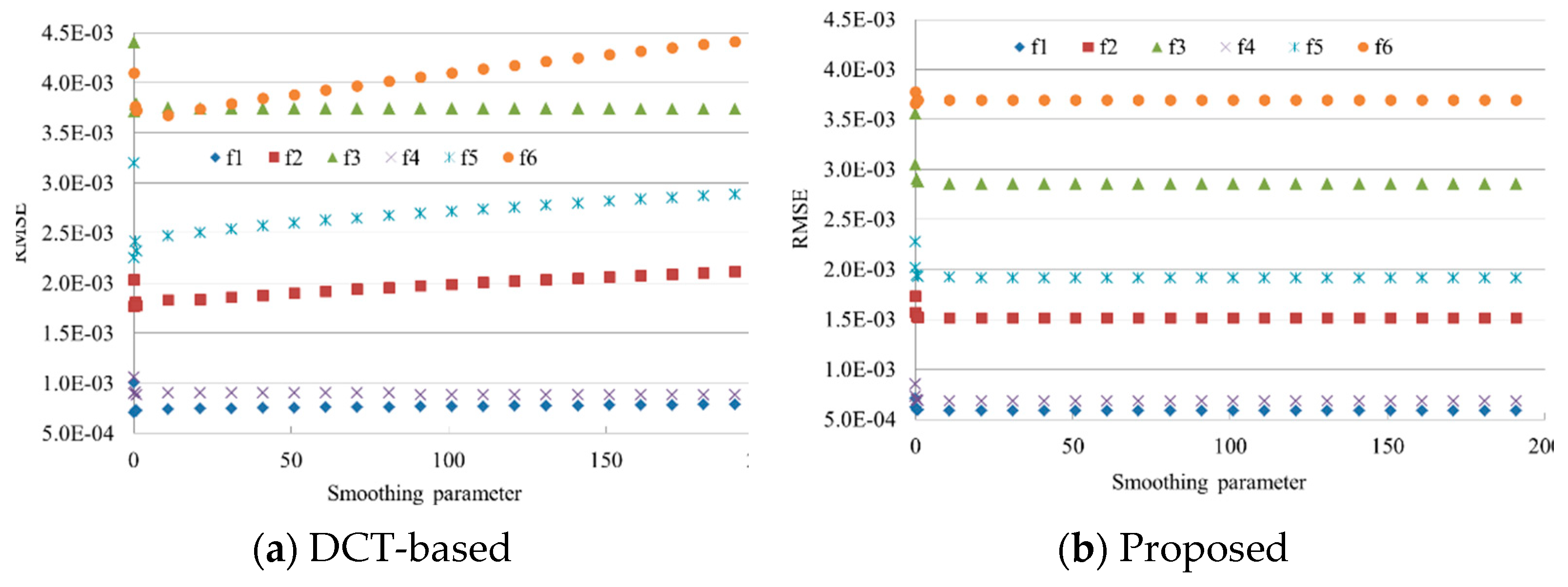
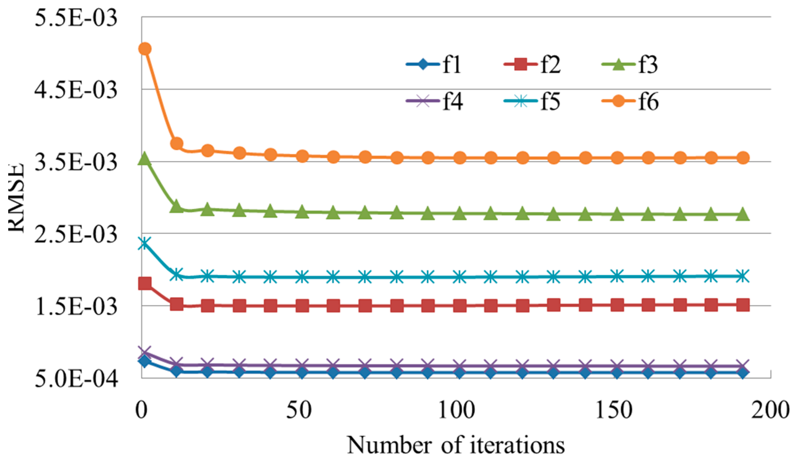
In the process of parameter determination, we tested different combinations. Specifically, the number of neighbors ranges from 15 to 40 with the step of 5 for IDW and OK. The power value of IDW varies from 1 to 5 with the step of 1. The smoothing parameters of the proposed method and the DCT-based TPS are , and the number of iterations of the proposed method is 20. Moreover, the smoothing parameter of the DCT-based method was also determined by the generalized cross-validation. Hereafter, for ease of discussion, DCT-based TPS with the parameter determined by trial-and-error and generalized cross-validation were termed DCT-T and DCT-G, respectively. NN and the linear interpolation do not require any parameters.
5.2.1. Public Dataset
Ten benchmark datasets with different terrain characteristics, provided by the International Society for Photogrammetry and Remote Sensing (ISPRS) Commission III [
42], were used to analyze the interpolation accuracy of the proposed method. Since the point labels (i.e., ground or nonground) in the dataset were known beforehand, only the ground points were used to produce DTMs. Firstly, the ground points were randomly divided into training and testing points consisting of 90% and 10% of points, respectively, then the former was used to produce DTMs and the latter to assess the DTM accuracy.
Table 4 gives the numbers of training points (#training) and testing points (#testing), area, and average point space for each sample. In addition, the standard deviation (STD) of elevations for describing terrain characteristic was also provided. Results exhibit that the 10 samples with different areas have various terrain complexities. Hengl [
43] indicated that a signal can be reconstructed if the sampling frequency is twice that of the original frequency. Thus, a cell size that keeps the majority of the information inherent in the original point dataset should be half the average point space between the closest point pairs. In addition, cell sizes of 0.25 m, 0.5 m, or 1.0 m are commonly used for lidar-derived DTMs in practice. Thus, based on the theory and practice, the optimal cell size for each sample is given in
Table 4.
Interpolation results (
Figure 6) show that terrain characteristics have a significant effect on the interpolation accuracy. Specifically, regardless of interpolators, s-21 and s-31, which are less complex than the other samples, have higher accuracy, while s-11 with the greatest complexity obtains the lowest accuracy. Among the interpolation methods, DCT-G tends to produce the poorest results in almost all samples, except for s-41. DCT-T always yields better results than DCT-G. This indicates that the generalized cross-validation method is unreliable for the determination of the smoothing parameter in practice. OK performs best in 9 out of 10 samples, and the proposed method is approximately as accurate as OK.
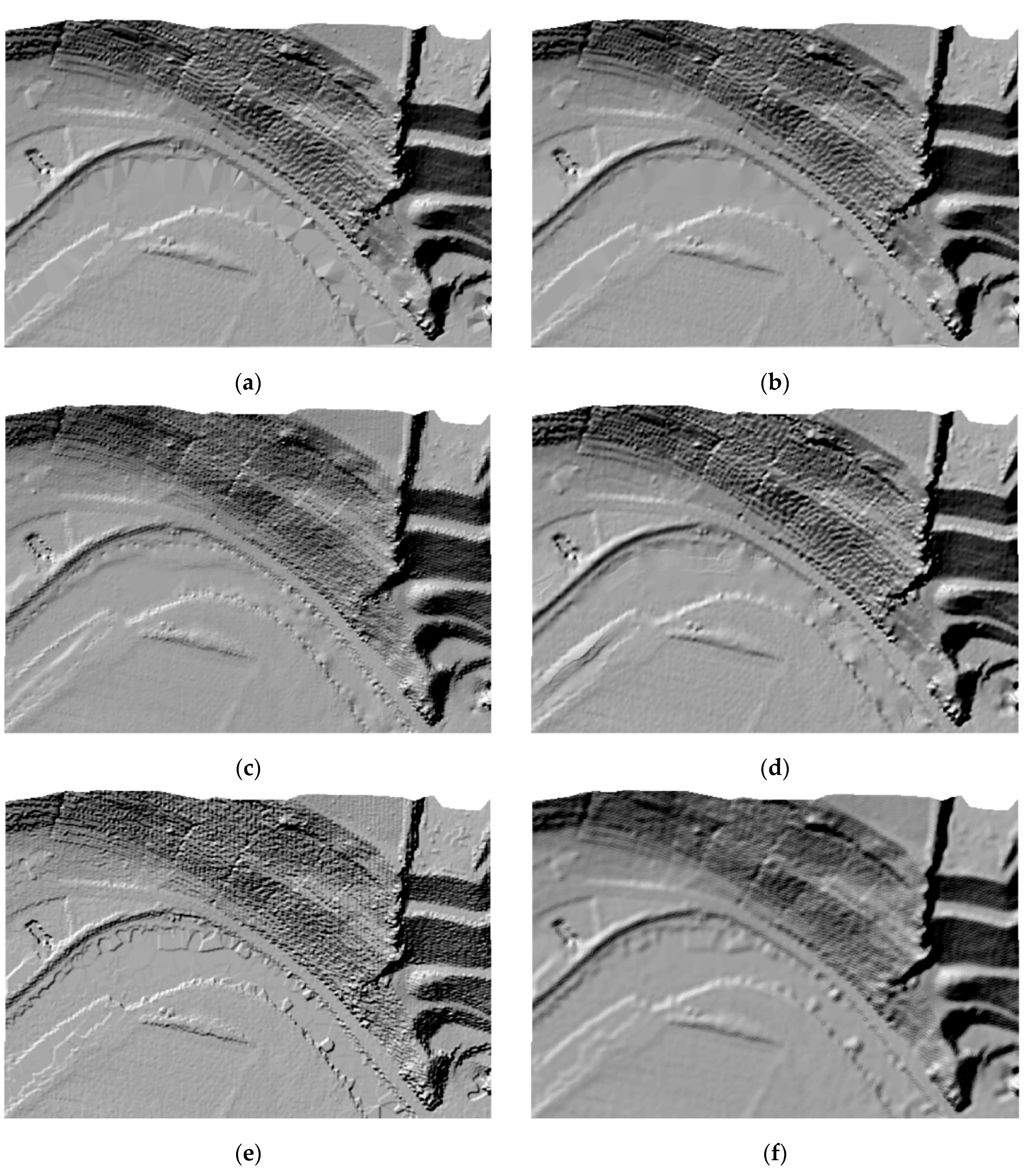
S-52 is taken as a representative to visually show the interpolated surfaces of all the methods, as this sample is characterized by a complex landscape including flat terrain, steep slopes, and break lines. Shaded relief maps show that the linear interpolation produces faceted surfaces where the sample density is low (
Figure 7a). This is because the linear method cannot handle complex terrain with nonlinear features. NN has sporadic outliers in the steep slopes due to its exact interpolation nature (
Figure 7b). IDW suffers from strips and pits in areas of steep slopes and flat areas (
Figure 7c). OK seems to generate a smooth surface, yet it has tree root-like discontinuities in the flat area because of its local interpolation nature (
Figure 7d). DCT-G has many bumps in the flat area and generates coarse surfaces in the steep slopes (
Figure 7e). The bumps of the DCT-G disappear in the surface of DCT-T, yet the steep slopes of the latter are blurred (
Figure 7f). The poor performance of the two DCT-based TPSs may be caused by their high sensitivity to the smoothing parameter, whose value was not optimally tuned. The proposed algorithm produces the most visually appealing surface, which is generally smooth and free of obvious artifacts (
Figure 7g). The good performance of the proposed method is thanks to the global interpolation manner and insensitivity to the smoothing parameter.
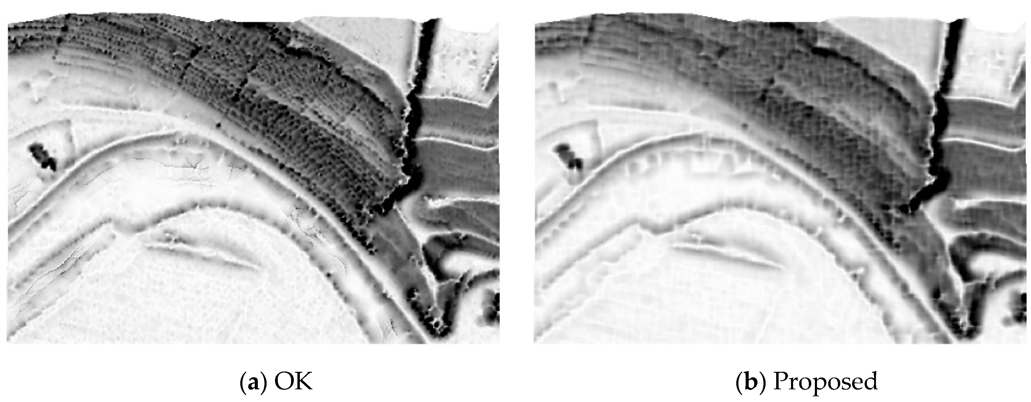
Although shaded relief map is a widely accepted technique for visually showing DTMs, it has two major drawbacks: Identifying details in deep shades and inability to properly represent linear features lying parallel to the light beam. In comparison, sky-view factor can be used as a general relief visualization technique to show relief characteristics [
44,
45]. Thus, the sky-view factors of OK and the proposed method on s-52 are demonstrated in
Figure 8. They are produced with Relief visualization Toolbox (
https://www.zrc-sazu.si/en/rvt). Obviously, OK surfers from tree-like discontinuities in the flat terrain (
Figure 8a), which is inconspicuous in the shaded relief map (
Figure 7d). However, these discontinuity features are avoided by the proposed method (
Figure 8b).
The rasterization time of all the methods on the 10 samples are shown in
Table 5. The time includes the costs for reading sample points, DTM interpolation, and storage transfer from random-access memory to the disk. Results demonstrate that irrespective of samples, the OK method has the largest computational time. Linear interpolation and NN are slightly faster than IDW since the former do not require the search of neighbors. In comparison, the proposed and the DCT-based methods are faster than the other methods. On average, the proposed method has the highest speed and is about 83 times as fast as OK. Note that compared to the DCT-based method, the efficiency of the proposed method is less obvious on the real-world dataset than on the simulated one. This is because saving DTMs from the random-access memory to the disk is much more time-consuming than solving the linear system of TPS.
Random access memory costs of all the methods on the samples are shown in
Table 6. Irrespective of the sample, the proposed method always has the least memory requirement, and OK has the largest. On average, the cost of the proposed method is about 1.14, 1.14, 10.62, 172.98, and 4.44 times less than those of the linear, NN, IDW, OK, and DCT-based methods, respectively.
5.2.2. Private Dataset
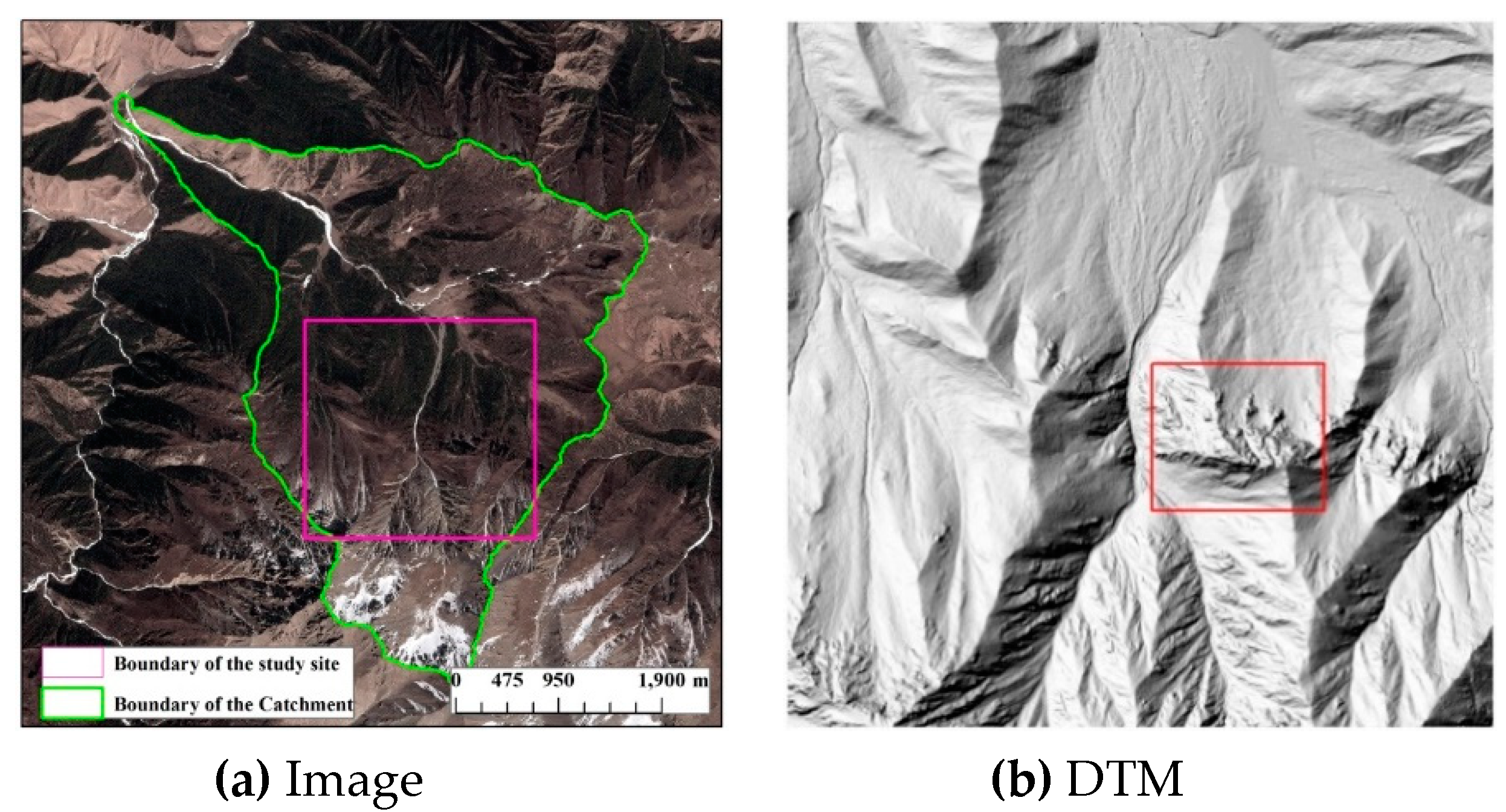
The study site is mainly located in Tianlaochi Catchment, Gansu province, China (
Figure 9). It covers an area of 2100 × 2100 m
2 with the mean elevation and the standard deviation of 3353.8 m and 239.4 m, respectively. Raw LiDAR data in the study site was captured using Leica ALS70 with the laser wavelength of 1064 nm and absolute flying height of 4800 m in July 2012. TerraScan, one of the main applications in the Terrasolid Software, was used to automatically filter the raw LiDAR point cloud. Then, the filtered points were manually edited with the help of orthoimages to assure the filtering accuracy. After that, 2,090,337 ground points and 4,189,499 nonground points were obtained. Like the process for handling the public dataset, 90% and 10% of ground points were, respectively, used as the training and testing data. The average point space of the training points is about 1.5 m. Thus, the desired DTM resolution should be 0.75 m. In addition to interpolation methods, sample density also has a significant influence on DTM accuracy [
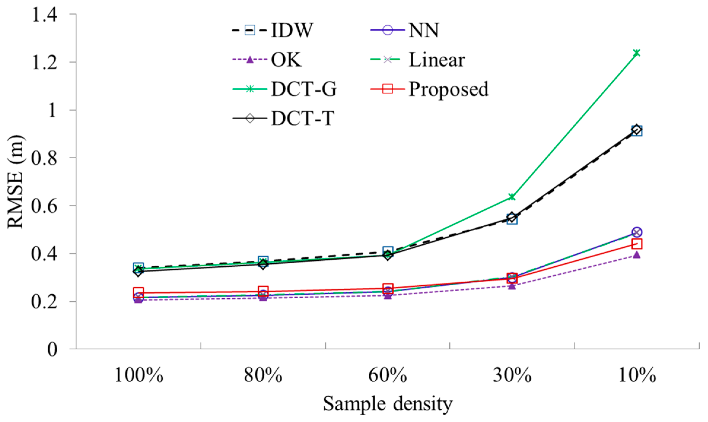
7]. Thus, we used different proportions of training samples to generate DTMs, namely 100%, 80%, 60%, 30%, and 10%.
Results (
Figure 10) demonstrated that as sample density decreases, the accuracies of all methods become lower. This conclusion is apparent as lower sample density means less captured terrain information. Regardless of sample density, OK consistently ranks the first, which is closely followed by the proposed method, linear, and NN. DCT-G always ranks the last. Although DCT-T performs slightly better than DCT-G, the former has much lower accuracy than the proposed method. This indicates that DCT is less reliable than the Gauss–Seidel method for solving the linear system of TPS in the real-world applications.
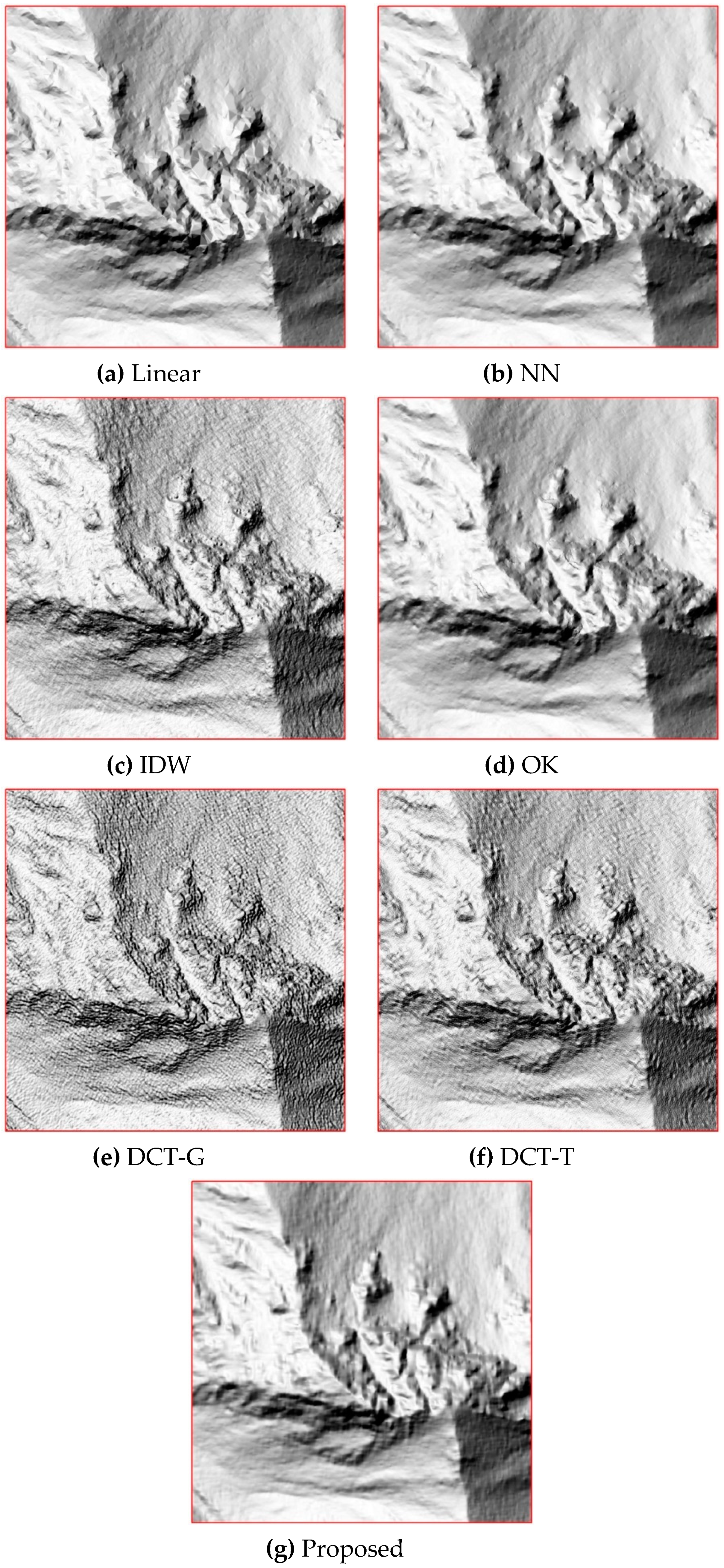
Figure 11 shows the shaded relief maps of all the interpolation methods on the 30% of training points in the area denoted by the red rectangle in
Figure 9b. We can see that linear interpolation (
Figure 11a) and NN (
Figure 11b) have obvious peak-cutting problems in the ridges. This result is mainly due to the fact that the two methods cannot estimate peaks or valleys that occur beyond the elevation range limits of a given same dataset [
10]. IDW produces a coarse surface because it is an exact interpolator (
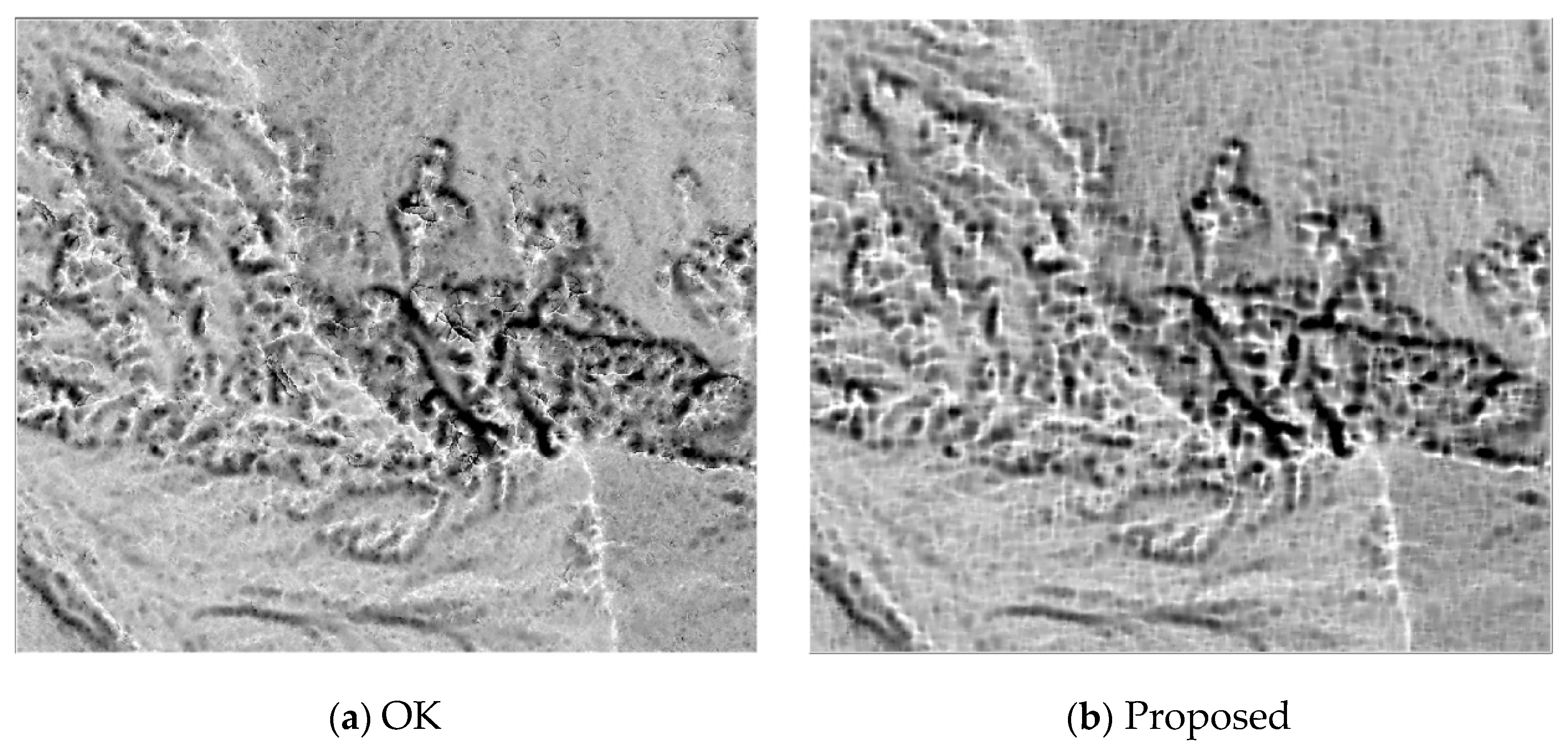
Figure 11c). It seems that OK generates a smooth surface, yet it suffers from discontinuities in some ridges because of the local interpolation nature (
Figure 11d). This is clearly demonstrated with its positive openness map (
Figure 12a), which was also produced with the Relief visualization Toolbox (
https://www.zrc-sazu.si/en/rvt). The two versions of DCT-based methods generate very coarse surfaces, caused by their sensitivity to the smoothing parameter and its improper estimation (
Figure 11e,f). In comparison, the proposed method obtains the most visually pleasing surface, where the terrain features are accurately preserved and the noise is smoothed out (
Figure 11g). In addition, compared to OK, the discontinuity features cannot be found in the positive openness map of the proposed method (
Figure 12b), which is mainly attributed to its global interpolation manner.
The computational costs (
Table 7) show that OK is extremely more time-consuming than the other methods. The proposed and DCT-based methods have faster speeds, which are closely followed by linear, NN, and IDW. These conclusions are consistent with that from the public dataset of this paper.
Table 8 shows the random-access memory costs of all the interpolation methods. Results indicate that regardless of data proportion, the proposed method has similar memory costs to linear and NN, and less than IDW and DCT-T. OK has the largest costs, which is 2.32 G on average. It is about 16.6 times as large as that of the proposed method.


