Anomaly Detection for Hyperspectral Imagery Based on the Regularized Subspace Method and Collaborative Representation

Abstract

Most of the conventional anomaly detectors only take advantage of the spectral information and do not consider the spatial information within neighboring pixels. Recently, the spectral-spatial based local summation anomaly detection (LSAD) algorithm has achieved excellent detection performances. In order to obtain various local spatial distributions with the neighboring pixels of the pixels under test, the LSAD algorithm exploits a multiple-window sliding filter, which can be computationally expensive and time-consuming. In this paper, to address these issues, two modified LSAD-based methods are proposed. The first method, called local summation unsupervised nearest regularized subspace with an outlier removal anomaly detector (LSUNRSORAD), is based on the concept that each pixel in the background can be approximately represented by its spatial neighborhood. The second method, called local summation anomaly detection based on collaborative representation and inverse distance weight (LSAD-CR-IDW), uses the surrounding pixels collected inside the outer window, while outside the inner window, to linearly represent the test pixel and introduces collaborative representation and inverse distance weight to further improve the computational speed and detection precision, respectively. The proposed methods were applied to a synthetic dataset and three real datasets. The experimental results show that the proposed methods have a better detection accuracy and computational speed when compared with the LSAD algorithm and others.

1. Introduction

Hyperspectral remote sensing images have a high spectral resolution and their hundreds of narrow contiguous bands, of about 10 nm wide, can be used to obtain a wealth of spectral information about target objects. Thus, hyperspectral remote sensing images are widely used in the field of target detection. Since it is difficult to obtain enough prior knowledge to characterize the statistical information of target categories, detection without a prior spectral information of the target, which is called “anomaly detection”, has been of significant interest [1,2]. Anomaly detection involves modeling the background and using the difference between the pixels and the background to detect anomalous pixels. In the field of hyperspectral remote sensing, anomaly detection has been widely applied to detect the locations of crop stress in precision farming [3,4], to locate scarce minerals [5], to analyze oil and environmental pollution [6], and to detect landmines for public safety [5].

Many different anomaly detection algorithms have been proposed. The classical detection algorithm, known as the Reed-Xiaoli (RX) [7] detector, was developed by Reed and Xiaoli in 1990 and can be considered as the benchmark for the performance evaluation of hyperspectral anomaly detectors. The RX detector is a second-order matched filtering algorithm that calculates the Mahalanobis distance of a test pixel and the background. When the entire image is considered for background modeling, this is known as global RX (GRX). If the RX detector estimates the background using local statistics, it is referred to as local RX (LRX) [8,9,10]. In real hyperspectral imagery, the background information is very complicated and cannot be described with just a multivariate normal distribution and it can be difficult to use the estimated covariance and mean vector to represent the background statistics, because of the existence of noise and anomalies. Under such circumstances, improved algorithms, such as weighted RX (W-RXD) [11] and linear filter based RXD (LF-RXD) [11], aim at increasing the probability of anomaly detection by improving the estimation of the background statistics. Some kernel-based detection algorithms, such as the classical nonlinear kernel RX [12] detection algorithm, have also achieved better anomaly detection performances than the conventional algorithms.

In recent years, methods based on sparse representation of signals have been applied to hyperspectral image target detection [13,14,15]. These methods aim to use as few background and target signals as possible to concisely represent the entire image information in an overcomplete dictionary composed of the background information and target information [16]. However, these methods only consider the spectral information and do not consider the spatial information, which makes it difficult to obtain a satisfactory detection performance. The collaborative-representation-based detector (CRD) [17] for hyperspectral anomaly detection is directly based on the concept that each background pixel can be approximately represented by its spatial neighborhood, whereas anomalies cannot, and has achieved satisfactory detection performances. Compared with the CRD algorithm, the collaborative representation-based with outlier removal anomaly detector (CRBORAD) [18] method, which removes outlier pixels that are significantly different from the majority of pixels, has further improved the detection accuracy. Liu et al. developed a multiple-window anomaly detector [19] to capture different levels of local spectral variations. It makes use of multiple windows with varying sizes to characterize and interpret the anomalous targets of various sizes. It adopts a successive nested-anomaly detector with windows nested in its preceding window. Different from the model, the local summation anomaly detection (LSAD) [20] method, proposed by Du et al., makes full use of the various local spatial distribution information of the neighboring pixels of a test pixel by using the local-window summation strategy, which greatly improves the detection accuracy. However, there are still some shortcomings. Firstly, the statistics of the background information are vulnerable to anomalous targets when using a single local window, which leads to a high false alarm rate. Secondly, the LSAD algorithm has the drawback of high computational complexity.

To solve these problems, we propose the local summation unsupervised nearest regularized subspace with an outlier removal anomaly detector (LSUNRSORAD) and the local summation anomaly detection based on collaborative representation and inverse distance weight (LSAD-CR-IDW) methods to improve the detection accuracy and the computational speed of the LSAD method, respectively.

In the LSAD algorithm, a covariance matrix is used to represent the correlation information between different background pixels and covariance inversion is used in the operation. However, the computation cost of matrix inversion is relatively high. In this paper, we propose two methods which use the linear combination of vector addition and multiplication to replace the complex matrix inversion. The proposed LSUNRSORAD method uses an outlier removal strategy to eliminate the influence of anomalous targets, and adopts an unsupervised nearest regularized subspace method to approximately represent its test pixels. Different from the CRBORAD algorithm, in the LSUNRSORAD method, we use the unsupervised nearest regularized subspace (UNRS) algorithm instead of the CRD algorithm to solve the convex optimization problem, and use the dual-window local summation strategy to make full use of the local background statistics information. This strategy is different from the single window local summation strategy in the LSAD [20] algorithm, in which, when the anomalous object is larger, the inner window can be used as a guardian window to restrict the contamination of the background pixel by the anomalous object. In the proposed LSAD-CR-IDW method, the local summation strategy is also used to make full use of the various local spatial distribution information of the neighboring pixels of the pixels under test. Meanwhile, in order to make full use of the spectral similarity information between the local background pixels, we try to introduce the inverse distance weight (IDW) [21] of surveying and the Tikhonov regularization [17,22] into collaborative representation method to improve the accuracy of linear representation.

The residual image is generated by subtracting the predicted background from the original image, and the anomalies can then be detected in the residual image. The detection results can be assessed using receiver operating characteristic (ROC) [23] curves and area under curve (AUC) [23] values. We evaluated and compared the proposed methods using a synthetic dataset and three real datasets. The results show that the proposed methods provide higher detection accuracies than the traditional methods. The rest of this paper is organized as follows. In Section 2, the proposed methods and the main concepts are presented. Section 3 describes the experiments undertaken to evaluate the proposed methods. Finally, Section 4 draws our conclusions.

2. Proposed Methods

In this section, we introduce the proposed LSUNRSORAD and LSAD-CR-IDW methods. In Section 2.1, we provide a short review of the UNRS [22] algorithm and the collaborative representation (CR) [17] algorithm, which are important techniques used in the proposed approach. We then explain the proposed methods in detail in Section 2.2.

2.1. The Unsupervised Nearest Regularized Subspace (UNRS) Algorithm

We let a given hyperspectral image dataset $X\in {ℝ}^{d\times N}$ be expressed as follows:

$$X={\left\{x_i\right\}}_{i=1}^N,$$

(1)

where $N$ is the total number of image pixels and each i-th column of $X$ corresponding to $x_i$ is a d-dimensional vector in the image. For each test pixel, $y\in {ℝ}^d$, which is a d-dimensional column vector, we assume that an approximation $y^{\prime }$ calculated via the linear combination of the surrounding selected data can be expressed as follows:

$$y^{\prime }=X_s\alpha ,$$

(2)

where $X_s$ is the surrounding background pixels and $\mathsf{\alpha }$ is the weight vector. The equation $X_s={\left\{x_i\right\}}_{i=1}^s\in {ℝ}^{d\times s}$ represents the surrounding background pixels collected inside the outer window while outside the inner window, in which each i-th column of $X_s$ corresponds to $x_i$ and $s$ is the number of chosen surrounding background pixels between the dual windows, which can be calculated by the following:

$$s=wi{n}_{out}\times wi{n}_{out}-wi{n}_{in}\times wi{n}_{in},$$

(3)

where $wi{n}_{out}$ denotes the size of the outer window and $wi{n}_{in}$ denotes the size of the inner window. In Equation (2), $\alpha \in {ℝ}^{s\times 1}$ is the weight vector. If we want to calculate $y^{\prime }$, the weight vector $\alpha$ must be known. Therefore, Equation (2) is converted to find the sum-to-one constraint weight vector $\alpha$, which minimizes the objective function [22] as follows:

$$f\left(\alpha \right)=\Vert y-X_s\alpha {\Vert }_2^2=\Vert y-{{\displaystyle \sum }}_{i=1}^s{\alpha }_i{x}_i{\Vert }_2^2,$$

(4)

where ${\alpha }_i$ is a i-th element of vector $\alpha$ and ‖*${\Vert }_2^2$ denotes the square of 2-norm. The original space is then “shifted” via centering $y$ to mean zero. The objective function $f\left(\alpha \right)$ can then be calculated by the following:

$$f\left(\alpha \right)=\Vert {{\displaystyle \sum }}_{i=1}^s{\alpha }_i\left(x_i-y\right){\Vert }_2^2=\Vert {{\displaystyle \sum }}_{i=1}^s{\alpha }_i{z}_i{\Vert }_2^2={\alpha }^{T}Z{Z}^T\alpha ,$$

(5)

where $z_i=x_i-y\in {ℝ}^{d\times 1}$, $Z\in {ℝ}^{s\times d}$, and $Z{Z}^T\in {ℝ}^{s\times s}$ is a symmetric matrix called the Gram matrix, denoted by $G$. In order to estimate the weight vector $\alpha$, we use a Lagrange multiplier to solve the function under the sum-to-one constraint condition. Hence, the cost function can be expressed as follows:

$$L\left(\alpha ,{\lambda }_0\right)={\alpha }^{T}G\mathsf{\alpha }-{\lambda }_0\left(1^T\alpha -1\right),$$

(6)

where $1$ is the $s\times 1$ vector, in which all the elements are equal to 1, and it satisfies the constraint condition $1^T\alpha =1$. The value ${\lambda }_0$ is a constant. We further derive the $\alpha$ and ${\lambda }_0$ in Equation (6). We can then find the value of $\alpha$ with the sum-to-one constraint.

$$\alpha =\frac{{{\displaystyle \sum }}_{j=1}^s{G}^{-1}}{{{\displaystyle \sum }}_{i=1}^s{{\displaystyle \sum }}_{j=1}^s{G}^{-1}},$$

(7)

where i, j is the rows and columns of the matrix index. Note that matrix $G^{-1}\in {ℝ}^{s\times s}$. We apply this technique by adding the regularized term to the objective function $f\left(\alpha \right)$. Equation (5) can then be modified as follows:

$$f\left(\alpha ,\lambda \right)={\alpha }^{T}G\alpha +\lambda {\alpha }^T\alpha ,$$

(8)

where $\lambda$ is a constant. Thus, we convert the above problem to an equivalent problem, solved using the Lagrange multiplier method. Taking the derivative, we can obtain the value of $\alpha$, which minimizes the new cost function as follows:

$$\alpha =\frac{{{\displaystyle \sum }}_{j=1}^s{\left(G+\lambda I\right)}^{-1}}{{{\displaystyle \sum }}_{i=1}^s{{\displaystyle \sum }}_{j=1}^s{\left(G+\lambda I\right)}^{-1}},$$

(9)

where $I$ is an identity matrix.

2.2. Collaborative Representation (CR)

We adopt collaborative representation [17] to linearly represent the test pixel, instead of using UNRS. Therefore, the problem of solving the weight vector $\alpha$ becomes the following:

$$L\left(\alpha ,{\lambda }_1\right)=argmi{n}_{\alpha }\Vert y-X_s\alpha {\Vert }_2^2+{\lambda }_1\Vert \alpha {\Vert }_2^2,$$

(10)

where ${\lambda }_1$ is the Lagrange multiplier. We also use a Lagrange multiplier to solve the objective function. Hence, Equation (10) is changed to the following:

$$L\left(\alpha ,{\lambda }_1\right)=argmi{n}_{\alpha }\left[{\alpha }^T\left(X_{s }^T{X}_s+{\lambda }_{1}I\right)\alpha -2{\alpha }^T{X}_{s }^{T}y\right],$$

(11)

and the solution is as follows:

$$\alpha ={\left(X_{s }^T{X}_s+{\lambda }_{1}I\right)}^{-1}{X}_{s }^{T}y.$$

(12)

We control the weight of the penalty norm by adjusting parameter ${\lambda }_1$. However, in the background pixels, some of the pixels will be very similar to the test pixel. Therefore, the weight should be increased in the linear representation and the weight should be reduced for dissimilar pixels. Tikhonov regularization [17,18,22,24] is introduced to adjust the weight as follows:

$${\Gamma }_y=\left[\begin{array}{ccc}\Vert y-x_1{\Vert }_2& \cdots & 0\\ ⋮& \ddots & ⋮\\ 0& \cdots & \Vert y-x_s{\Vert }_2\end{array}\right].$$

(13)

The objective function after adding the Tikhonov regularization can be converted to the following:

$$L\left(\alpha ,{\lambda }_1\right)=\arg {\min }_{\mathsf{\alpha }}\Vert y-X_s\alpha {\Vert }_2^2+{\lambda }_1\Vert {\Gamma }_y\alpha {\Vert }_2^2.$$

(14)

The final solution is obtained by the Lagrange multiplier, as follows:

$$\alpha ={\left(X_{s }^T{X}_s+{\lambda }_1{\Gamma }_y^T{\Gamma }_y\right)}^{-1}{X}_{s }^{T}y.$$

(15)

Under the sum-to-one constraint condition, Equation (15) is converted to the following:

$$L\left(\alpha ,{\lambda }_1\right)=\arg {\min }_{\alpha }\Vert y_2-X_s^{\prime }\alpha {\Vert }_2^2+{\lambda }_1\Vert {\Gamma }_y\alpha {\Vert }_2^2,$$

(16)

where $y_2=\left[y;1\right]$, $X_s^{\prime }=\left[X_s;1\right]$. In the vector $y_2$ and matrix $X_s^{\prime }$, $1$ is a row vector with all elements equal to 1. By using the Lagrange multiplier method, the final solution can be obtained as follows:

$$\alpha ={\left(X_{s }^{\prime T}{X}_s^{\prime }+{\lambda }_1{\Gamma }_y^T{\Gamma }_y\right)}^{-1}{X}_{s }^{\prime T}{y}_2.$$

(17)

We can obtain the residual image by Equation (17) after the representation process is completed.

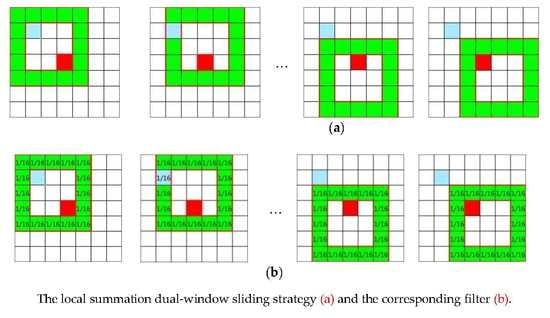
2.3. Local Summation Unsupervised Nearest Regularized Subspace with an Outlier Removal Anomaly Detector (LSUNRSORAD)

The presence of outliers affects the detection accuracy and the outliers cannot be represented by neighboring pixels. In order to further improve the detection accuracy, we introduce an outlier removal strategy to the UNRS algorithm. Pixels with intensity values greater than the maximum threshold or smaller than the minimum threshold are considered to be outliers (e.g., the pink square in Figure 1a). The outliers in the dual windows that are clearly different from the other pixels are removed based on certain thresholds [18], which are constructed by using the mean and standard deviation of the intensity values of the pixels within the dual windows. The intensity values here are obtained by accumulating the radiance values of all bands in the hyperspectral image. The setting of threshold is based on the knowledge of mathematical statistics. It is assumed that the background of imagery obeys the normal distribution and, when the confidence interval is 95%, we can get the threshold, as presented in Equations (18) and (19).

$${\tau }_{max}=\mu +2\times \sigma ,$$

(18)

$${\tau }_{min}=\mu -2\times \sigma ,$$

(19)

where $\mu$ and $\sigma$ are the mean and standard deviation of the background pixels $X_s$, and ${\tau }_{max}$ and ${\tau }_{min}$ represent the maximum and minimum of the background pixels’ intensities, respectively. Pixels with intensity values greater than ${\tau }_{max}$ or less than ${\tau }_{min}$ are removed. Therefore, $X_s$ can be replaced by $X_s^{\prime }$, in which $s^{\prime }$ is the number of background pixels after outlier removal and $X_s^{\prime }$ is used to predict the test pixel $y^{\prime }$. Once the representation process (Figure 1b) is completed, we can obtain the residual image by:

$$r_1=\Vert y-y^{\prime }{\Vert }_2=\Vert y-X_s^{\prime } {\alpha }^{\prime }{\Vert }_2,$$

(20)

where ${\alpha }^{\prime }$ is the new weight vector after removing the outliers and $r_1$ is the distance value. If the distance $r_1$ is larger than the threshold, then $y$ is declared an anomalous pixel. For a test pixel, the traditional detection algorithms exploit only one local window to estimate the local background statistics. Du et al. [20] put forward a local summation single-window sliding strategy (in Figure 2), which can take full advantage of the local background statistics. We borrow from this idea and put forward the local summation dual-window sliding strategy shown in Figure 3. When the inner window size is three and the outer window size is five, we need to calculate a nine ($wi{n}_{in}\times wi{n}_{in}$) times linear representation (Figure 1b) after the sliding window operation is completed. We then need to calculate the result by the following:

$$r={{\displaystyle \sum }}_{i=1}^{wi{n}_{in}\times wi{n}_{in}}{r}_i.$$

(21)

The surrounding pixels collected inside the outer window while outside the inner window are used for estimating the local background statistics information, while the inner window is used to constrain anomalous targets. Meanwhile, the sliding strategy is used to accurately represent the local background statistics by local dual-window summation.

As shown in Figure 4, the light blue square represents the anomalous pixel. If we use only one dual window to estimate the test pixel and we assume that the weights of each surrounding pixel are the same (all 1/16), then the probability of whether the test pixel is an anomalous pixel is determined by its surrounding pixels. If all surrounding pixels are anomalous pixels, the probability of the test pixel being anomalous pixel is 1 ($16\times 1/16$) and if 8 surrounding pixels are anomalous pixels, then the probability of the test pixel is $1/2$ ($8\times 1/16$), so the probability of a test pixel with 1/16 is determined as an anomalous pixel. However, the proposed local summation dual-window sliding strategy can make full use of the background distribution information around the test pixel. As shown in Figure 5, when the inner window size is three and the outer window size is five, we can obtain nine dual windows after the window sliding is completed, of which only three dual windows contain anomalous pixels. Therefore, $1/3$ of the windows contain an anomalous pixel. The probability of a test pixel with 1/16 is determined as an anomalous pixel in each window, so the testing pixel is the probability of an anomalous pixel to 1/48 ($1/3\times 1/16$), in our proposed method. The overall description of the LSUNRSORAD method is given in Algorithm 1.

Algorithm 1: The LSUNRSORAD Algorithm.

Input: Hyperspectral data $X={\left\{x_i\right\}}_{i=1}^N$, window size ($wi{n}_{out},wi{n}_{in}$), and parameter λ

for all pixels do

for each window do

(1) For each test pixel y, a 2D matrix is constructed based on the pixels within the dual window by $X_s={\left\{x_i\right\}}_{i=1}^s$;

(2) Remove outlier pixels in matrix $X_s$ according to Equation (18) and Equation (19);

(3) Calculate the weight vector ${\alpha }^{\prime }$ by Equation (9);

(4) Calculate the detection result of each window measurement by Equation (20);

end for

(5) Calculate the final detection result by Equation (21);

end for

Output: Anomaly detection map

2.4. Local Summation Anomaly Detection Based on Collaborative Representation and Inverse Distance Weight (LSAD-CR-IDW)

In order to make full use of the local background statistics information, the local summation dual-window sliding strategy is used. The traditional local RX algorithm [8,9,10] exploits only one local window to estimate the local background statistics, which cannot suppress the global background. However, the LSAD algorithm, proposed by Du et al. [20], exploits a local summation single-window sliding strategy to suppress the global background. The strategy is shown in Figure 2. We take a $3\times 3$ size single window for illustration purposes. For each test pixel, we can obtain nine windows using the single-window sliding strategy. The nine local windows are then used for implementation of the second-order Mahalanobis distance features of the test pixel as follows:

$$di{s}_{M_i}={\left(y-{\mu }_i\right)}^T{{\displaystyle \sum }}_{i=1}^{k\times k}\left(y-{\mu }_i\right),$$

(22)

where $y$ is the test pixel, ${\mu }_i$ is the i-th mean vector of $X_s{}_i$ $\left(i=1, 2,\cdots ,k\times k\right)$, and $X_s{}_i$ is the local background pixels of local sliding windows. The value $k$ is the size of the inner window and $k\times k$ is the number of local sliding windows. Finally, all of the Mahalanobis distances $di{s}_M$ are summed as the detected values of the test pixel as follows:

$$r_{LSAD}={{\displaystyle \sum }}_{i=1}^{k\times k}di{s}_{M_i},$$

(23)

where $r_{LSAD}$ is the final detection result. Differing from the local summation single-window sliding strategy, we propose the local summation dual-window sliding strategy shown in Figure 3. In Figure 2, for each test pixel, we can obtain $k\times k$ windows using the local summation single-window sliding strategy. However, when the neighboring pixels contain an anomalous target and more than one pixel, the background statistics are easily contaminated when using only a single local window for anomaly detection, which leads to a high false alarm rate.

As shown in Figure 3, through the local summation dual-window sliding strategy, the surrounding pixels collected inside the outer window while outside the inner window are used for estimating the local background statistics information of the test pixel, while the inner window as a guard window is used to constrain the anomalous targets, so as not to take into account potential anomalous target pixels in the local background characterization. With respect to the size of the internal window, it is usually set to the maximum radius of the anomalous targets, in the case of prior knowledge, so that the anomalous targets can be included in the inner window, as much as possible, to exclude their influence on the surrounding pixels. As shown in Figure 3, we adopt the local summation dual-window sliding strategy to accurately represent the local background statistics of the test pixel. In order to improve the speed of computational speed, we adopt collaborative representation [17] to linearly represent the test pixel, instead of using UNRS. Considering that the closer the test pixel is the higher the similarity between the background pixel and the test pixel will be, the inverse distance weight (IDW) [21] is selected to make the most of the space-varying information. The relatively pure background pixel can be obtained using the CRD method. Then, we add the IDW to the representation process, replacing the weight ${\Gamma }_y$ in Equation (14) with $W_1$.

$$W_1={\Gamma }_y\times IDW,$$

(24)

where $y$ and $\xi$ denote the test pixel $\left(i,j\right)$ and any pixel $\left(k,l\right)$ of $X_s$, respectively, then the $IDW$ can be expressed by the following:

$$IDW\left(x,\xi \right)=\frac{h_i{}^{-p}}{{{\displaystyle \sum }}_{i=1}^s{h}_i{}^{-p}},$$

(25)

$$h_i=\sqrt{{\left(i-k\right)}^2+{\left(j-l\right)}^2},$$

(26)

where $h_i$ represents the Euclidean distance of geometric coordinates and $p$ is a constant that is set to be 2. Then, we can also employ the technique to obtain the weight vector $\alpha$. We can get the final weight vector $\alpha$ by solving Equation (16):

$$\alpha ={\left(X_{s }^{\prime T}{X}_s^{\prime }+{\lambda }_1{W}_1{}^T{W}_1\right)}^{-1}{X}_{s }^{\prime T}{y}_2.$$

(27)

Finally, we can obtain the residual image by Equation (20) after the representation process is completed. As in the LSUNRSORAD method, we use the local summation dual-window sliding strategy. Finally, we can obtain the detection result by summing the results of each window by Equation (21). The description of the LSAD-CR-IDW method is given in Algorithm 2.

Algorithm 2: LSAD-CR-IDW Algorithm

Input: Three-dimensional hyperspectral cube $X\in R^d$, window size $\left({\mathrm{win}}_{\mathrm{out}},{\mathrm{win}}_{\mathrm{in}}\right)$, and parameter $\lambda ;$

for all pixels do

for each window do

(1) For each test pixel $y$, a 2D matrix is constructed based on the pixels within the dual window by $X_s={\left\{x_i\right\}}_{i=1}^s$;

(2) Calculate the weight vector $\alpha$ for each window by Equation (27);

(3) Calculate the detection result of each window by Equation (20);

end for

Calculate the final detection result by Equation (21);

end for

Output: Anomaly detection map

3. Experiments and Analysis

In this section, in order to evaluate the effectiveness of the proposed methods, we compare the results derived by the proposed methods with those derived by five other methods, as follows: GRX, LRX, UNRS, CRD, and LSAD. We conducted experiments on four hyperspectral images. One experiment based on a real hyperspectral imagery dataset was used as a simulated experiment to analyze the property of the proposed methods, and the other experiments were real data experiments to demonstrate the effectiveness of the different methods. It is worth noting that these first three datasets were obtained after preprocessing, including atmospheric correction, and the first three datasets are widely used in the field of anomaly detection. The fourth dataset obtained was after MODTRAN atmospheric correction. 2-D binary plots are used to illustrate the detection results. For a numerical comparison, we use the ROC curves and AUC values as the main criteria to evaluate the detection results.

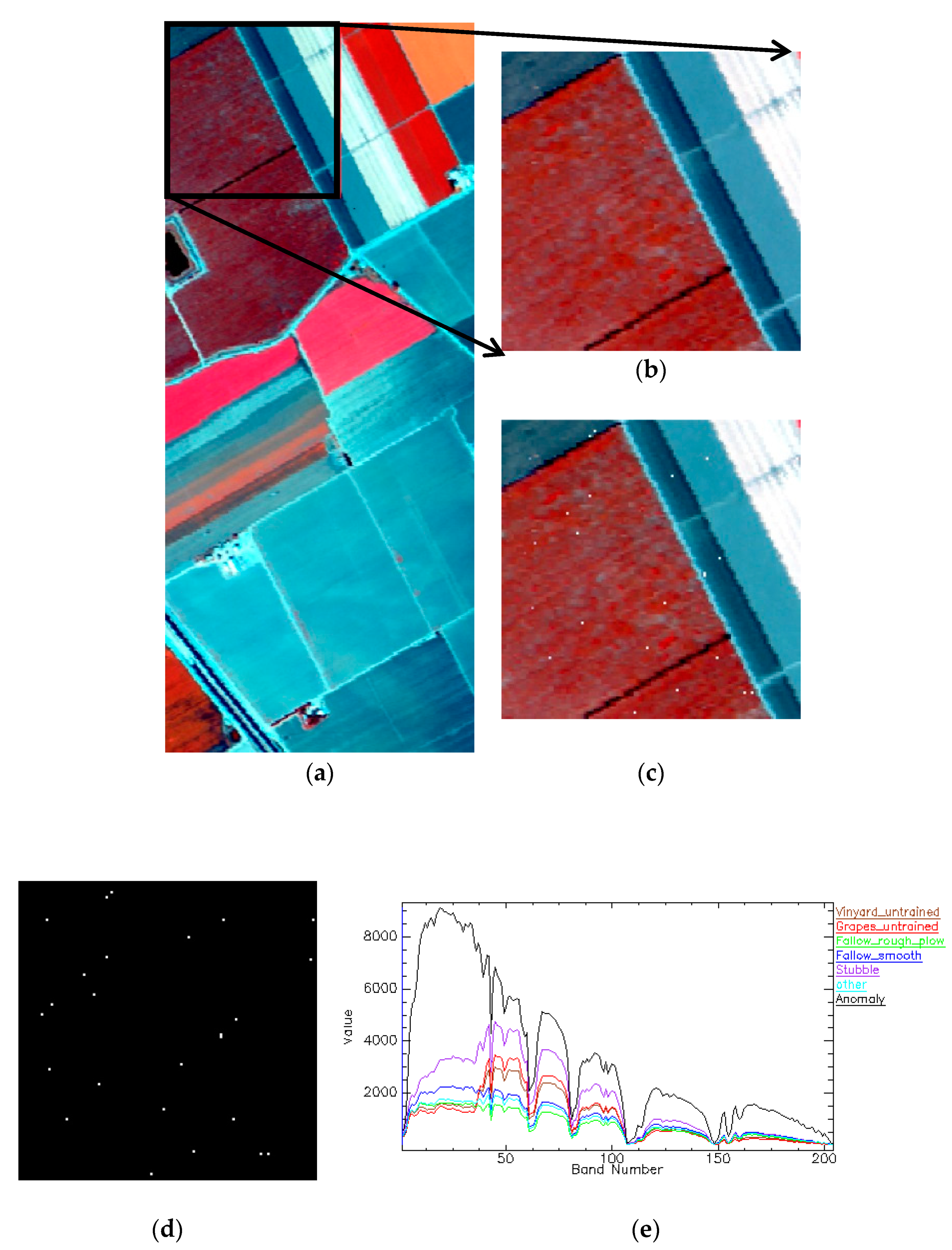
3.1. Synthetic Data Experiment

3.1.1. Synthetic Data Description

The first hyperspectral dataset is synthetic data that were generated based on an Airborne Visible/Infrared Imaging Spectrometer (AVIRIS) [25] data from the Salinas Valley, CA, USA. It can be downloaded from the GIC website [26]. The original data set (Figure 6a), comprising vegetables, bare soil, and vineyard fields, consists of $512\times 217$ pixels with 224 bands, with a spatial resolution of 3.7 m. After removing 20 atmospheric and water vapor absorption bands (108–112, 154–167, and 224), sub-images of size $120\times 120$ were cropped (Samples: 1 to 120, Lines: 1 to 120), as depicted by the red square frames in Figure 6b. The target implantation method [27] was applied to implant anomalous targets into the AVIRIS Salinas sub-images (Figure 6c). We employed RX detection of the whole-image to find the pixels which were different from the others as the anomalous target spectra of the synthetic data. By detecting the whole image with the RX detector, we have found that the most prominent objects are buildings, so we set the building spectral as the anomalous spectral in Figure 6e. The performance of the detectors could be evaluated in a fully controlled environment through the method of target embedding. The buried target spectra needed to have a large difference from the background spectra of the cropped area. Figure 6e shows the spectral curves of the anomalous targets and the spectral curves of the main objects in the background (Figure 6c). In this simulated experiment, in order to be similar to the anomalous target distribution of a real image, 25 pixels were randomly selected as the anomalous target distribution points. Based on the linear mixing model, a synthetic subpixel anomaly target was generated as follows:

$$z=f\times t+\left(1-f\right)\times b$$

(28)

where $z$ is the spectrum of the synthetic subpixel anomaly target, $f$ is the specified abundance fraction, ranging from 0.04 to 1 with a step size of 0.04, $t$ is the anomalous spectra, and $b$ is the background spectra.

3.1.2. Parameter Analysis

The initial choices of various parameters are important for the proposed algorithms. For this simulated dataset, we adopt the target embedding method to fully control the generating environment of sub-pixel anomalous targets. In the UNRS, CRD and two proposed methods, the constant $\lambda$ is a tradeoff parameter. In order to find the suitable $\lambda$, we first fix the other parameters (e.g., $wi{n}_{out}=5$ and $wi{n}_{in}=3$) and merely adjust the value of $\lambda$. As shown in Figure 7, when the value of $\lambda$ varies from 0.01 to 100, the detection results of different methods can be seen. The comparison results show that the two proposed methods have apparently better detection results than other methods, regardless of the value of $\lambda$.

Table 1. The AUC values in the Salinas dataset with different $\lambda$ parameters.

	Methods	UNRS	CRD	LSUNRSORAD	LSAD-CR-IDW
$\mathit{\lambda }$
0.01		0.92497	0.92712	0.99999	0.99998
0.1		0.92497	0.92712	0.99996	0.99998
1		0.92496	0.92712	0.99985	0.99994
10		0.92496	0.92712	0.99952	0.99993
100		0.92491	0.92712	0.99925	0.99988

reveals that the detection results of different methods are optimal when parameter $\lambda$ equals to 0.01.

Since the choice of internal and external window sizes has an enormous impact on the results, we first set parameter $\lambda$ = 0.01 and set different window sizes to explore the optimal window size to show the superiority and fully excavate the potential of the proposed methods. In order to obtain the optimal window size, the AUCs are calculated under different window sizes with the synthetic dataset, as shown in Figure 8. We can conclude that the proposed LSUNRSORAD method is the most robust and the accuracy of the proposed two methods is generally higher than that of other detection methods.

3.1.3. Detection Performance

To verify the effectiveness of the proposed methods, we compared the proposed methods with GRX, LRX, UNRS, CRD, and LSAD. For a numerical comparison, we use receiver operating characteristic (ROC) [23] curves and area under the curve (AUC) [23] values as the main criteria to evaluate the detection results. In the experiment, we used a notebook computer with Windows 7 OS, an Intel Core(TM) i3-2350 CPU @ 2.30 GHz, and 4 GB RAM. The codes are run by MATLAB^® 2016b. In different methods, the choice of initial parameters is very important.

The window size has a great influence on the operation time of different detection algorithms. In order to highlight the superiority of the proposed algorithms in the computational cost, we try to set the window size to be the same in different methods to ensure that the algorithms are at the same condition. The parameters used in these methods are shown in

Table 2. Parameters of different detection methods.

Methods	Parameters
GRX	—
LRX	$wi{n}_{out}=5$, $wi{n}_{in}=3$
UNRS	$wi{n}_{out}=5$, $wi{n}_{in}=3$, and $\lambda =0.01$
CRD	$wi{n}_{out}=5$, $wi{n}_{in}=3$, and $\lambda =0.01$
LSAD	$win=5$
LSUNRSORAD	$wi{n}_{out}=5$, $wi{n}_{in}=3$, and $\lambda =0.01$
LSAD-CR-IDW	$wi{n}_{out}=5$, $wi{n}_{in}=3$, and $\lambda =0.01$

. It is worth noting that we adopt the edge expansion method [20] to fill the boundary in order to ensure no absence of detection on the edge of image.

For the Salinas dataset, the detection results of the different methods are displayed as 3D images in Figure 9. Figure 10a shows the separability [25,28,29,30] between anomalous targets and the background, and the output value range of the different detection methods. In each group, the first bar is a red target bar representing the range of the anomalous targets and the second is a cyan background bar representing the range of the background. The interval between the red box and the cyan box represents the separability between anomalous target pixels and background pixels. As shown in Figure 10a, the UNRS, CRD, LSAD, LSUNRSORAD, and LSAD-CR-IDW methods show the better separability between anomalies and background, while the ranges of the background for LSAD are larger than the ranges of the others. It indicates that the two proposed methods can restrict the range of the background to a smaller range, which enables the anomalies to be clearer in the detection map. In Figure 10, compared with the LSAD method, the proposed methods are more capable of identifying the synthetic subpixel anomalous targets, which makes it easier to find a suitable threshold and use threshold segmentation method to convert grayscale images to binary images.

As shown in Figure 10b and

Table 3. Comparison of AUC and execution times using the Salinas dataset.

Method	GRX	LRX	UNRS	CRD	LSAD	LSUNRSORAD	LSAD-CR-IDW
AUC	0.80732	0.99160	0.92497	0.92712	0.99987	0.99999	0.99998
Time/s	0.59	190.01	8.7	11.7	2603.4	76.08	65.15

. Comparing the ROC curves in Figure 10b and the AUC values in Table 3, we can see that the proposed methods obtain better results than the other methods. The LSAD method is more accurate than the GRX, LRX, UNRS, and CRD methods, but it takes the longest time to calculate. The LSUNRSORAD and LSAD-CR-IDW methods offer better results than LSAD and the computational cost is relatively low compared to the LSAD method.

For the simulated dataset, we adopt the target embedding method to fully control the generating environment of sub-pixel anomalous targets. The detection results indicate that the proposed methods show better performances in the subpixel targets’ detection.

3.2. Real Data Experiments

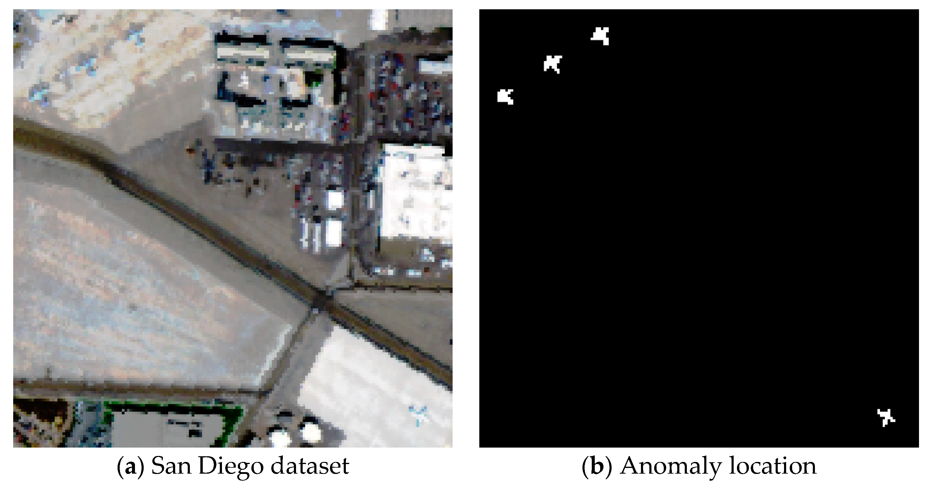
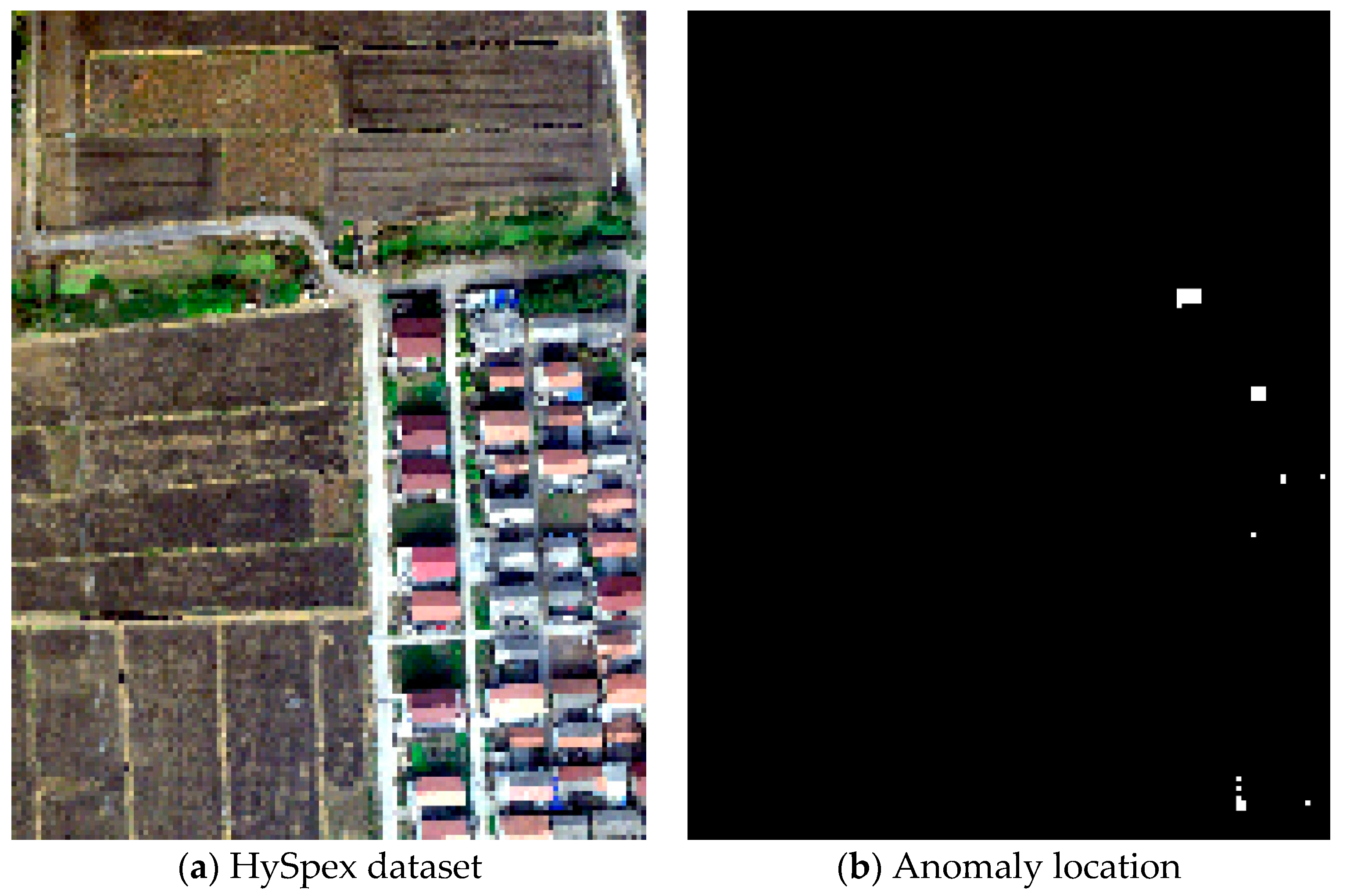
3.2.1. Real Datasets Description

The second datum is a real hyperspectral image used in the experiments, which featured a part of San Diego airport in the USA. This image was acquired by the AVIRIS sensor [16,29,31,32,33,34], with a spatial resolution of 3.5 m. In the experiment, 189 bands of the raw data were retained after removing the corresponding water vapor bands and low signal-to-noise ratio (SNR) bands. The whole image size is 400 rows × 400 columns × 189 bands, and a 170 × 170 × 189 region (samples: 42 to 211, lines: 1 to 170) was cropped for the experiment. The whole image and the target map of the anomalies in the test region [18,35] are shown in Figure 11. The sub-image contains 4 airplanes with 106 anomalous pixels, and it comes from Reference [36].

The third dataset was provided by professor Paolo Gamba from the Telecommunications and Remote Sensing Laboratory, Pavia University, Italy. It can be downloaded from the GIC website [26]. The scenes are Pavia Centra scenes, and it was acquired by the Reflective Optics Spectrographic Imaging System airborne instrument (ROSIS). The image has a geometric resolution of 1.3 m and contains 115 bands with the wavelength ranging from 430 nm to 860 nm. After removal of the noisy bands, 102 bands are retained. The experiment was performed using sub-regions of $120\times 200$ size (samples: 224 to 423, lines: 1 to 120) with a ground truth of the anomalies (Figure 12). The main backgrounds in the image are water and a bridge and the main anomalous targets are vehicles on the bridge with 43 pixels. The anomaly map comes from Reference [37].

The last dataset used in the real-world experiments was a HySpex hyperspectral dataset obtained from an aircraft platform in November 2014. This is a strip image covering an agricultural area of the Quanshan District of Xuzhou, China, including 160 visible wave bands and 288 shortwave infrared spectral bands ranging from 415 nm to 2508 nm, with a spatial resolution of 0.73 m. After spectral and spatial resampling, the number of spectral bands was 200 and the spatial resolution was 1.5 m. The sub-images of size $170\times 130$ were cropped from the strip image and the outliers in the sub-images mainly come from the colored steel roofs. The scene and the ground truth of the anomalies are shown in Figure 13.

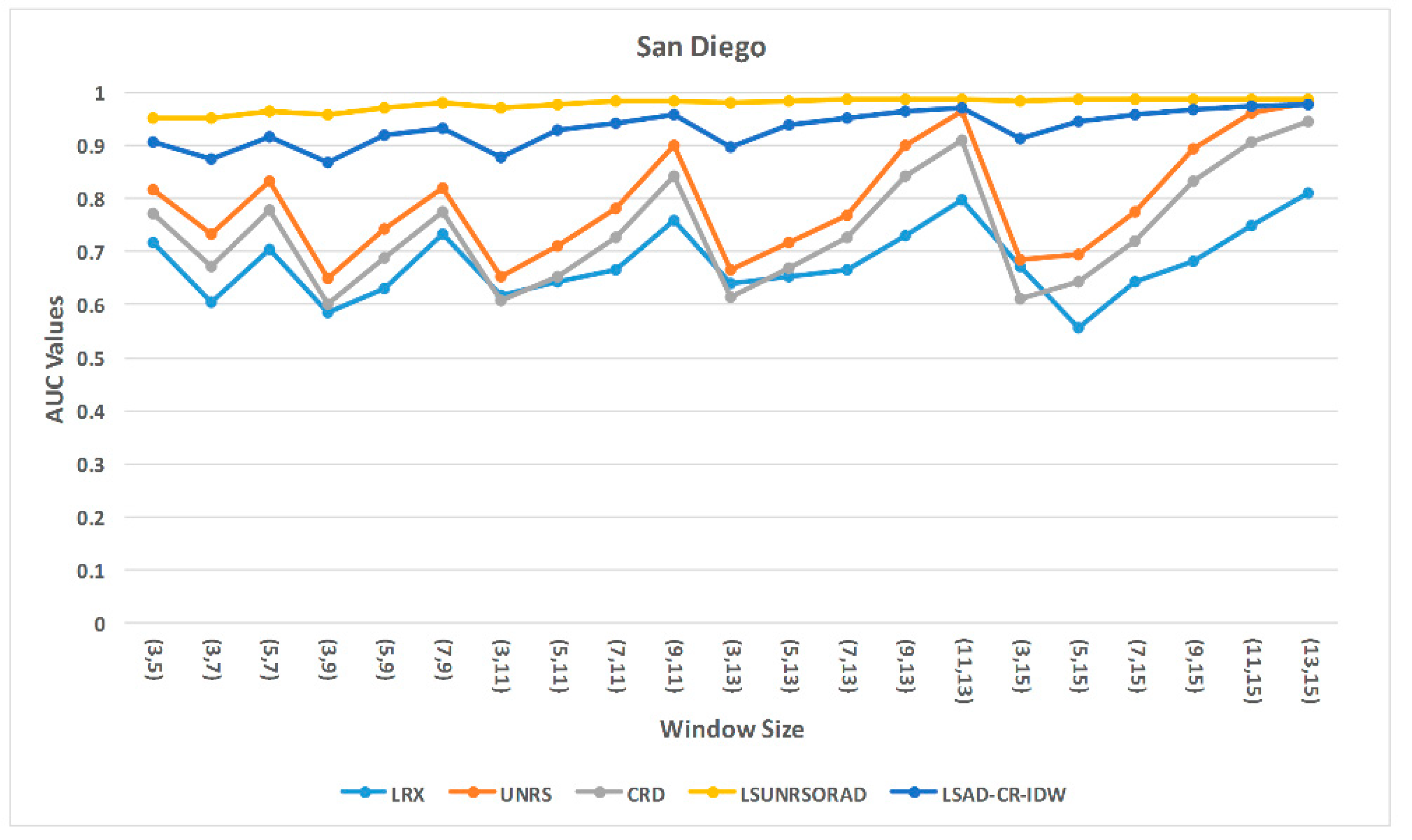
3.2.2. Parameter Analysis

As previously mentioned, as the initial choices of various parameters are important for these methods, we use trial-and-error method to find the optimal parameters of different methods. To find the suitable $\lambda$, we first fix $wi{n}_{out}=5$ and $wi{n}_{in}=3$ and merely adjust the value of $\lambda$. As shown in Figure 14, the detection results of four methods are listed, in which we can find the optimal $\lambda$ values of different detection methods. From Figure 14, we can conclude that the proposed LSAD-CR-IDW method is sensitive to parameter $\lambda$, while the proposed LSUNRSORAD method is the most robust.

Similarly, we set the optimal parameter $\lambda$ for different methods as shown in

Table 4. The optimal parameter $\lambda$ of different detection methods.

	Method	UNRS	CRD	LSUNRSORAD	LSAD-CR-IDW
Datasets
San Diego	$\lambda$	0.01	100	100	100
Pavia	$\lambda$	100	100	100	100
Hyspex	$\lambda$	0.01	0.01	0.1	100

and then set the different window sizes to explore the optimal window size to show the superiority and fully excavate the potential of the proposed methods. The Figure 15, Figure 16 and Figure 17 shows the AUC values of different methods under different window sizes. It is worth noting that the proposed two methods have approximate detection results, so the curves used to represent the two methods in Figure 16 almost coincide. Therefore, from these figures we can conclude that the proposed LSUNRSORAD and LSAD-CR-IDW methods are the most robust and the accuracies of the proposed two methods are higher than that of other detection methods.

3.2.3. Detection Performance

From the numerical value of the ordinate axis, in this synthetic data experiment, the parameter $\lambda$ has little effect on the detection results of the UNRS, CRD, LSUNRSORAD and LSAD-CR-IDW. However, in the real hyperspectral images, the parameter $\lambda$ has an enormous influence on LSAD-CR-IDW method. When the anomalous object is large, the parameter $\lambda$ needs to be set a larger value to balance the influence of penalty item. So, we set the empirical parameter here. The empirical value of parameter $\lambda$ is 100 in the LSAD-CR-IDW. To effectively evaluate the computational cost of the proposed methods, we try to keep all the parameters the same in different methods and the others parameters are shown in Table 2. It is worth noting that these parameters are not optimal. We only use these same parameters to evaluate the computational cost of different methods.

The 3D detection results for the three real datasets (the San Diego, the Pavia Centra and the Hyspex datasets) are shown in Figure 18, Figures 20 and 22. Figure 19, Figures 21 and 23 show the statistical separability analyses and the ROC curves of the corresponding datasets.

Table 5. Comparison of AUC values and execution times of the different methods for the three real datasets.

Dataset		GRX	LRX	UNRS	CRD	LSAD	Method1	Method2
San Diego	AUC	0.73369	0.71684	0.8173	0.77195	0.79681	0.91284	0.9073
	Time /(s)	1.15	336.03	13.81	14.28	5120.27	154.02	133.74
Pavia	AUC	0.99553	0.94957	0.98489	0.97960	0.95954	0.99862	0.99931
	Time /(s)	0.53	71.78	9.42	9.41	1178.55	125.49	106.17
HySpex	AUC	0.83484	0.76179	0.74988	0.81177	0.73731	0.83955	0.86486
	Time /(s)	0.86	257.99	10.19	10.62	3996.17	161.60	122.07

lists the AUC values and the execution time of the different methods for the real datasets.

As shown in Figure 19a, the separability between anomalous targets and the background indicate that both the proposed methods and others cannot effectively separate the background and anomalous features, which compress background and anomalous targets in a narrow range under complex background conditions. So, in Figure 18, the detection results of the San Diego dataset contain a large background.

As shown in Figure 18, under the same condition, we can find that GRX, LSUNRSORAD, and LSAD-CR-IDW methods can suppress the background better than others. Combined with Figure 19b, it can be seen that the detection accuracy of the GRX algorithm is relatively low. It indicates that the two proposed methods can separate background and anomalous objects better, which also enable the anomalies to be clearer in the detection map. Comparing the ROC curves in Figure 19b, we can also clearly find that the two proposed methods have better capabilities for identifying the anomalous targets than the other methods.

In the case of the Pavia Centra dataset, Figure 21a shows that the GRX, LRX, UNRS, and the two proposed methods can effectively limit the background value to a small interval, while the CRD and LSAD methods cannot. However, the LRX and UNRS methods cannot effectively separate the background and anomalous objects. The remaining three methods show a better separation between anomalies and backgrounds.

From Figure 20, we can clearly find that the proposed LSUNRSORAD and LSAD-CR-IDW methods can detect more pixels in the detection results and, compared with GRX, these two methods have relatively low false alarm rates. Figure 21b also illustrates that the proposed LSUNRSORAD and LSAD-CR-IDW methods have better results than the others.

As mentioned earlier, under complex background objects, it is not effective to recognize anomalous objects only by binary image, but we can see the suppression of the background by different detectors in the 3D detection results. In the experiment of Hyspex dataset, from Figure 22 and the Figure 23a, we can find that the GRX, LRX, and the proposed methods show better separability than the others. The ROC curve shows that the GRX and the proposed LSUNRSORAD and LSAD-CR-IDW methods have a better detection performance than the other methods.

It should be emphasized that in the three real hyperspectral images, we use the same window size and these parameters are not optimal. We only use these same parameters to evaluate the computational cost of different methods. For a numerical comparison, we use area under the curve (AUC) values as the main criteria to evaluate the detection results, as shown in Table 5. As can be seen from Table 5, the two proposed methods offer better results than the LSAD method, with less computational costs in the three real datasets.

By using this local summation dual-window sliding strategy, we can effectively utilize the surrounding spatial information around the test pixels. When the window size remains the same, the proposed method can often achieve better detection results than the traditional methods. Compared with the LSAD method, the improved methods have higher precision and shorter running time, while keeping the same external window size.

Overall, the proposed methods show a better performance than the other methods. Compared with the LSAD method, the two proposed methods provide better results in anomaly detection accuracy. The proposed LSUNRSORAD and LSAD-CR-IDW methods reduce the calculation cost and improve the operation speed, while ensuring the accuracy of the detection results. Therefore, the proposed LSUNRSORAD and LSAD-CR-IDW methods will be of practical use in real applications.

4. Discussion

In this paper, the potential gain of the proposed methods in Table 1 is low when the value of λ varies from 0.01 to 100. The reason for the low gain is related to the synthesis of an anomalous image. Since the background features of the images are relatively simple, the anomalous targets we selected are relatively prominent, and the synthesized anomalous targets are pixel-level small target. Therefore, the detection accuracy of various algorithms for anomalies is relatively high, which weakens the influence of regularization parameters on detection results.

By analyzing the results of four groups of experimental data, we have found the fact that, in our proposed two methods, the influence of parameter λ on detection algorithms may be related to the size of anomalous targets. When the size of anomalous targets is larger, the detection results will be better only when the regularization parameters become larger. Under different regularization parameters, the detection performance of the proposed two methods is still better than that of the UNRS and CRD algorithms, which also show the stability of the proposed methods relative to parameter λ.

5. Conclusions

In this paper, we have proposed the LSUNRSORAD and LSAD-CR-IDW methods of anomaly detection for hyperspectral imagery, which take full advantage of the local background distribution of every local window for the test pixel of the hyperspectral image. We adopt the UNRS method to obtain the weight vector in the LSUNRSORAD method and we use an outlier removal strategy to alleviate the interference of outliers. In the proposed LSAD-CR-IDW method, we propose a dual-window sliding strategy to reduce the probability of contamination of the test pixel and we introduce collaborative representation to improve the speed of operation. Furthermore, in order to make the most of the space-varying information, we introduce the inverse distance weight commonly used in surveying and mapping.

The experiments undertaken in this study confirm that the proposed methods have a better performance than the traditional anomaly detection methods. However, the computational cost of the proposed LSUNRSORAD and LSAD-CR-IDW methods are still enormous, which will be the focus of our future work.

References

1. Niu, Y.; Wang, B. Hyperspectral anomaly detection based on low-rank representation and learned dictionary. Remote Sens. 2016, 8, 289. [Google Scholar] [CrossRef]
2. Rejas Ayuga, J.G.; Martínez Marín, R.; Marchamalo Sacristán, M.; Bonatti, J.; Ojeda, J.C. Hyperspectral anomaly detection in urban scenarios. Int. Arch. Photogramm. Remote Sens. Spat. Inf. Sci. 2016, 41, 111–116. [Google Scholar] [CrossRef]
3. Meuleman, K.; Coppin, P.; Debacker, S.; Debruyn, W.; Nackaerts, K.; Scheunders, P.; Sterckx, S. Optimal hyperspectral indicators for stress detection in orchards. In Proceedings of the 3rd EARSel Wokrshop on Imaging Spectroscopy, Herrsching, Germany, 13–16 May 2003; Volume 2010, pp. 1381–1382. [Google Scholar]
4. Waheed, T.; Bonnell, R.B.; Prasher, S.O.; Paulet, E. Measuring performance in precision agriculture: CART—A decision tree approach. Agric. Water Manag. 2006, 84, 173–185. [Google Scholar] [CrossRef]
5. Makki, I.; Younes, R.; Francis, C.; Bianchi, T.; Zucchetti, M. A survey of landmine detection using hyperspectral imaging. ISPRS J. Photogramm. Remote Sens. 2017, 124, 40–53. [Google Scholar] [CrossRef]
6. Bu, Z.; Yu, Z.; Huo, S. Research on oil pollution image classification of airborne hyperspectral data based on spectral angle analysis method. In Proceedings of the International Conference on Information Science and Engineering, Hangzhou, China, 4–6 December 2011; pp. 3946–3949. [Google Scholar]
7. Reed, I.S.; Yu, X. Adaptive multiple-band CFAR detection of an optical pattern with unknown spectral distribution. IEEE Trans. Acoust. Speech Signal Process. 1990, 38, 1760–1770. [Google Scholar] [CrossRef]
8. Matteoli, S.; Diani, M.; Corsini, G. A kurtosis-based test to efficiently detect targets placed in close proximity by means of local covariance-based hyperspectral anomaly detectors. In Proceedings of the Hyperspectral Image and Signal Processing: Evolution in Remote Sensing (WHISPERS), 2011 3rd Workshop, Lisbon, Portugal, 6–9 June 2011; pp. 1–4. [Google Scholar]
9. Molero, J.M.; Garzón, E.M.; García, I.; Plaza, A. Analysis and optimizations of global and local versions of the RX algorithm for anomaly detection in hyperspectral data. IEEE J. Sel. Top. Appl. Earth Obs. Remote Sens. 2013, 6, 801–814. [Google Scholar] [CrossRef]
10. Taitano, Y.P.; Geier, B.A.; Bauer, K.W. A locally adaptable iterative RX detector. EURASIP J. Adv. Signal Proce. 2010, 11, 341908. [Google Scholar] [CrossRef]
11. Guo, Q.; Zhang, B.; Ran, Q.; Gao, L.; Li, J.; Plaza, A. Weighted-RXD and linear filter-Based RXD: Improving background statistics estimation for anomaly detection in hyperspectral imagery. IEEE J. Sel. Top. Appl. Earth Obs. Remote Sens. 2014, 7, 2351–2366. [Google Scholar] [CrossRef]
12. Kwon, H.; Nasrabadi, N.M. Kernel RX-algorithm: A nonlinear anomaly detector for hyperspectral imagery. IEEE Trans. Geosci. Remote Sens. 2005, 43, 388–397. [Google Scholar] [CrossRef]
13. Zhao, R.; Du, B.; Zhang, L.; Zhang, L. A robust background regression based score estimation algorithm for hyperspectral anomaly detection. ISPRS J. Photogramm. Remote Sens. 2016, 122, 126–144. [Google Scholar] [CrossRef]
14. Wu, C.; Du, B.; Zhang, L. Hyperspectral anomalous change detection based on joint sparse representation. ISPRS J. Photogramm. Remote Sens. 2018, 146, 137–150. [Google Scholar] [CrossRef]
15. Soofbaf, S.R.; Sahebi, M.R.; Mojaradi, B. A sliding window-based joint sparse representation (SWJSR) method for hyperspectral anomaly detection. Remote Sens. 2018, 10, 434. [Google Scholar] [CrossRef]
16. Xu, Y.; Wu, Z.; Li, J.; Plaza, A.; Wei, Z. Anomaly detection in hyperspectral images based on low-rank and sparse representation. IEEE Trans. Geosci. Remote Sens. 2016, 54, 1990–2000. [Google Scholar] [CrossRef]
17. Li, W.; Du, Q. Collaborative representation for hyperspectral anomaly detection. IEEE Trans. Geosci. Remote Sens. 2015, 53, 1463–1474. [Google Scholar] [CrossRef]
18. Vafadar, M.; Ghassemian, H. Hyperspectral anomaly detection using outlier removal from collaborative representation. In Proceedings of the International Conference on Pattern Recognition and Image Analysis, Shahrekord, Iran, 19–20 April 2017; pp. 13–19. [Google Scholar]
19. Liu, W.M.; Chang, C.I. Multiple-window anomaly detection for hyperspectral imagery. IEEE J. Sel. Top. Appl. Earth Obs. Remote Sens. 2013, 6, 644–658. [Google Scholar] [CrossRef]
20. Du, B.; Zhao, R.; Zhang, L.; Zhang, L. A spectral-spatial based local summation anomaly detection method for hyperspectral images. Signal Process. 2016, 124, 115–131. [Google Scholar] [CrossRef]
21. Lu, G.Y.; Wong, D.W. An adaptive inverse-distance weighting spatial interpolation technique. Compt. Geosci. 2008, 34, 1044–1055. [Google Scholar] [CrossRef]
22. Li, W.; Du, Q. Unsupervised nearest regularized subspace for anomaly detection in hyperspectral imagery. In Proceedings of the Geoscience and Remote Sensing Symposium, Melbourne, Australia, 21–26 July 2014; pp. 1055–1058. [Google Scholar]
23. Hanley, J.A.; Mcneil, B.J. The meaning and use of the area under a receiver operating characteristic (ROC) curve. Radiology 1982, 143, 29. [Google Scholar] [CrossRef] [PubMed]
24. Li, W.; Tramel, E.W.; Prasad, S.; Fowler, J.E. Nearest regularized subspace for hyperspectral classification. IEEE Trans. Geosci. Remote Sens. 2013, 52, 477–489. [Google Scholar] [CrossRef]
25. Yuan, Y.; Wang, Q.; Zhu, G. Fast hyperspectral anomaly detection via high-order 2-D crossing filter. IEEE Trans. Geosci. Remote Sens. 2014, 53, 620–630. [Google Scholar] [CrossRef]
26. Hyperspectral Remote Sensing Scenes. Available online: http://www.ehu.eus/ccwintco/index.php?title=Hyperspectral_Remote_Sensing_Scenes (accessed on 22 May 2019).
27. Stefanou, M.S.; Kerekes, J.P. A method for assessing spectral image utility. IEEE Trans. Geosci. Remote Sens. 2009, 47, 1698–1706. [Google Scholar] [CrossRef]
28. Zhao, R.; Du, B.; Zhang, L. Hyperspectral anomaly detection via a sparsity score estimation framework. IEEE Trans. Geosci. Remote Sens. 2017, 55, 3208–3222. [Google Scholar] [CrossRef]
29. Zhang, Y.; Du, B.; Zhang, L.; Wang, S. A low-rank and sparse matrix decomposition-based mahalanobis distance method for hyperspectral anomaly detection. IEEE Trans. Geosci. Remote Sens. 2016, 54, 1376–1389. [Google Scholar] [CrossRef]
30. Du, B.; Zhang, L. Random-selection-based anomaly detector for hyperspectral imagery. IEEE Trans. Geosci. Remote Sens. 2011, 49, 1578–1589. [Google Scholar] [CrossRef]
31. Taghipour, A.; Ghassemian, H.; Mirzapour, F. Anomaly detection of hyperspectral imagery using differential morphological profile. In Proceedings of the 2016 24th Iranian Conference on Electrical Engineering (ICEE), Shiraz, Iran, 10–12 May 2016; pp. 1219–1223. [Google Scholar]
32. Li, J.; Zhang, H.; Zhang, L.; Ma, L. Hyperspectral anomaly detection by the use of background joint sparse representation. IEEE J. Sel. Top. Appl. Earth Obs. Remote Sens. 2015, 8, 2523–2533. [Google Scholar] [CrossRef]
33. Zhang, L.; Zhang, L.; Tao, D.; Huang, X. Sparse transfer manifold embedding for hyperspectral target detection. IEEE Trans. Geosci. Remote Sens. 2013, 52, 1030–1043. [Google Scholar] [CrossRef]
34. Xu, Y.; Wu, Z.; Xiao, F.; Zhan, T.; Wei, Z. A target detection method based on low-rank regularized least squares model for hyperspectral images. IEEE Geosci. Remote Sens. Lett. 2016, 13, 1129–1133. [Google Scholar] [CrossRef]
35. Vafadar, M.; Ghassemian, H. Hyperspectral anomaly detection using modified principal component analysis reconstruction error. In Proceedings of the Iranian Conference on Electrical Engineering, Tehran, Iran, 2–4 May 2017; pp. 1741–1746. [Google Scholar]
36. Ling, Q.; Guo, Y.; Lin, Z.; An, W. A constrained sparse representation model for hyperspectral anomaly detection. IEEE Trans. Geosci. Remote Sens. 2018, 57, 2358–2371. [Google Scholar] [CrossRef]
37. Zhu, L.; Wen, G. Hyperspectral anomaly detection via background estimation and adaptive weighted sparse representation. Remote Sens. 2018, 10, 272. [Google Scholar]
Figure 1. Outlier removal and the linear representation process: (a) the local dual-window; and (b) the process of linear representation. The red square represents the test pixel and the green squares represent the background pixels.
Remotesensing 11 01318 g001
Figure 2. The local summation single-window sliding strategy. The red square represents the test pixel.
Remotesensing 11 01318 g002
Figure 3. The local summation dual-window sliding strategy. The red square represents the test pixel.
Remotesensing 11 01318 g003
Figure 4. Schematic diagram of the dual-window strategy with anomaly (left) and the corresponding filter (right).
Remotesensing 11 01318 g004
Figure 5. The local summation dual-window sliding strategy (a) and the corresponding filter (b).
Remotesensing 11 01318 g005
Figure 6. Salinas dataset: (a) Pseudo-color image; (b) Sub-image; (c) Synthetic image; (d) Anomaly location; (e) Spectral curves of the main ground objects and anomalies.
Remotesensing 11 01318 g006
Figure 7. The influence of parameters λ on AUC value in the Salinas dataset.
Remotesensing 11 01318 g007
Figure 8. AUC values of different window sizes in the Salinas dataset.
Remotesensing 11 01318 g008
Figure 9. Detection results of the different methods using the Salinas dataset: the GRX, LRX, UNRS, CRD and LSAD are the comparative methods; LSUNRSORAD and LSAD-CR-IDW are our proposed two methods.
Remotesensing 11 01318 g009
Figure 10. Salinas dataset: (a) Statistical separability analysis. Method1 represents the LSUNRSORAD method and method2 represents the LSAD-CR-IDW method; (b) ROC curves.
Remotesensing 11 01318 g010
Figure 11. The San Diego airport hyperspectral data, showing the test region and the target map.
Remotesensing 11 01318 g011
Figure 12. The Pavia Centra dataset and the anomaly target map.
Remotesensing 11 01318 g012
Figure 13. The HySpex dataset and the anomaly target map.
Remotesensing 11 01318 g013
Figure 14. The influence of parameters λ on AUC value in the real dataset.
Remotesensing 11 01318 g014
Figure 15. AUC values of different window sizes in San Diego dataset.
Remotesensing 11 01318 g015
Figure 16. AUC values of different window sizes in Pavia Centra dataset.
Remotesensing 11 01318 g016
Figure 17. AUC values of different window sizes in the Hyspex dataset.
Remotesensing 11 01318 g017
Figure 18. Detection results of the different methods using the San Diego dataset: the GRX, LRX, UNRS, CRD and LSAD are the comparative methods; LSUNRSORAD and LSAD-CR-IDW are our proposed two methods.
Remotesensing 11 01318 g018
Figure 19. San Diego dataset. (a) Statistical separability analysis: Method1 represents the LSUNRSORAD method and method2 represents the LSAD-CR-IDW method; (b) ROC curves.
Remotesensing 11 01318 g019
Figure 20. Detection results of the different methods using the Pavia Centra dataset: the GRX, LRX, UNRS, CRD and LSAD are the comparative methods; LSUNRSORAD and LSAD-CR-IDW are our proposed two methods.
Remotesensing 11 01318 g020
Figure 21. Pavia Centra dataset: (a) Statistical separability analysis: Method1 represents the LSUNRSORAD method and method2 represents the LSAD-CR-IDW method; (b) ROC curves.
Remotesensing 11 01318 g021
Figure 22. Detection results of the different methods using the HySpex dataset: the GRX, LRX, UNRS, CRD and LSAD are the comparative methods; LSUNRSORAD and LSAD-CR-IDW are our proposed two methods.
Remotesensing 11 01318 g022
Figure 23. Hyspex dataset: (a) Statistical separability analysis: Method1 represents the LSUNRSORAD method and method2 represents the LSAD-CR-IDW method; (b) ROC curves.
Remotesensing 11 01318 g023