Auto Encoder Feature Learning with Utilization of Local Spatial Information and Data Distribution for Classification of PolSAR Image

Abstract

The distribution of data plays a key role in the designing of a machine learning model. Therefore, this paper proposes a novel auto encoder network based on the distribution of polarimetric synthetic aperture radar (PolSAR) data matrix. Designed specifically for PolSAR data matrix, the proposed mixture auto encoder (MAE) feature learning method defines data error term in the loss function according to the data distribution. Instead of the pixel itself, all pixels in the neighborhood are used as input to train the proposed MAE. Then, a corresponding classification network is also given by discarding the decoder process of the proposed MAE and connecting with a Softmax classifier. The MAE is trained using the unlabeled data, while the training process of the classification network is completed with the help of a small number of labeled pixels. In view of the phenomenon of misclassification in the predicted result image, two post-processing steps acting on local spatial are also given, which accomplished by the proposed two filters. Extensive experiments by four methods were made over three real PolSAR images including the proposed classification network. The experimental results show that introducing data distribution into the auto encoder network leads to an average 4% improvement in overall accuracy for three PolSAR images. Moreover, the post-processing steps with the proposed filters bring a new level of discrimination on the classification performance of PolSAR images.

1. Introduction

In the field of remote sensing, one of the most used and advanced sensors among radar imagery is SAR over the recent decades. It works in the microwave frequency range and utilizes the backscatter wave signals received from the observed region to supply various resolution images of the Earth surface. Relative to optical and spectral remote sensing system, the superiorities of SAR mainly consist of diversity polarization modes of emitting or receiving of polarized radar waves and the ability to work in all-weather conditions, such as fog and rain or day and night. Compared with microwave remote sensing image, optical remote sensing image has great advantages in many aspects, such as intuitive and easy to understand, relatively high spatial resolution and rich in content and the target structure features under sunny weather conditions. PolSAR image classification has always been one of the most elementary and significant applications in SAR image interpretation and target recognition. The PolSAR image used here is acquired by SAR sensors in all modes of polarization. The task of PolSAR image classification is allotting label to each pixel. As one of the most extensively used applications of SAR, PolSAR image classification has been studied for a long time. More attention has been paid to different kinds of methods to accomplish the task of PolSAR image classification. A great variety of methods has been put forward and received a sustained attention and development. The methods mainly consist of three categories: considering the statistical distribution of PolSAR data [1,2,3,4], combining with polarization target decomposition of PolSAR data [5,6,7] and utilizing machine learning [8,9,10]. Nevertheless, it remains a necessary approach to develop new and improve existing methods by utilizing the relevant information of PolSAR datasets. To solve the problem of PolSAR image classification better, a growing number of researchers have been devoted to work on the utilizing of different kinds of methods simultaneously. The proposed method mainly includes integrating the data distribution of PolSAR data matrix within machine learning. Aiming at the phenomenon of misclassification in the result images, a filter is proposed for post-processing based on the prior information provided by the confusion matrix. Another filter using only spatial location information is also given to further improve the visual effect of the resulting images.

Based on the complex Wishart distribution of covariance matrix or coherency matrix, Wishart distance, as proposed by Lee et al. [1], undoubtedly has been one of the most prominent research findings in the application of the statistical distribution of PolSAR data. Wishart classifier labels each pixel on the basis of minimizing the distance from the pixel to each center. It is obvious that the performance of Wishart classifier depends on the quality of the initial center of each class. In view of the mechanism of polarization scattering, several polarization decomposition methods have been put forward to classify the PolSAR image [5,6,7]. The typical representation method of them is H/$\alpha$ decomposition, which was presented by Cloude and Pottier [5]. The coherency matrix is decomposed into three components of different scattering mechanisms. It is an unsupervised classification method. Even though only eight categories can be distinguished, it is still extensively used for its simplicity and clearly physical meanings [11]. Moreover, polarization decomposition methods are often combined with statistical property of PolSAR image to accomplish the process of classification jointly. For example, Lee [2] obtained the result of H/$\alpha$ decomposition to initialize the classification of PolSAR image. The process of classification is carried out by repeatedly calculating the mean of pixels for each category and taking advantage of the Wishart distance to reclassify pixels in the PolSAR image.

As described above, these methods highly rely on the complex analysis of the PolSAR data, which is difficult and time consuming. Moreover, there is hardly any way to try to exploit the unlabeled pixels in the classification of PolSAR image for all these traditional methods. In fact, labeling the PolSAR image pixel by pixel is labor intensive. In most cases, most of the pixels are unlabeled, and only a few of the labeled pixels are available. Hence, it would be exciting if a large number of unlabeled pixels could be fully utilized.

As one of the most important and effective branches of artificial intelligence, the method of machine leaning is also applied in the classification of PolSAR image, such as support vector machine (SVM) [12,13] and neural networks (NNs) [14,15,16,17,18]. Although the machine learning can achieve better classification results, it depends heavily on the feature extraction process of pixels. It needs professional knowledge and plenty of experiments to determine which features should be selected and how to gain them better. The auto encoder (AE) network is a typical NN, which is trained to produce the output that approaches the input [19]. Since the information of interest is contained within the activation of hidden units, it can also be applied to extract the features of samples. In the loss function of AE, the similarity of the input and the output is measured with the Frobenius norm, which is suitable for natural images that obey the Gaussian distribution. As one of the most popular deep NNs, deep belief network was not extensive used until an efficient greedy learning algorithm [20] was proposed by Hinton et al. It performs well in many fields, including the speech recognition [21], image recognition [22] and natural language processing [23]. The machine learning methods above have been directly employed for the classification of PolSAR image. For example, LV models the PolSAR data by the general deep belief network (DBN) [24]. More and more attention has been paid to integrating the distribution characteristics of PolSAR data into machine learning methods in recent years. While taking the complex Wishart distribution of coherency matrix of PolSAR into account in the process of constructing the loss function of AE network, Xie et al. [25] presented a novel features extraction model, which called Wishart auto encoder model (WAE). It combines Wishart distance with the back propagation (BP) algorithm through the training procedure of AE. Generally speaking, features learned by WAE should be more suitable for the task of PolSAR image classification. In the same way, Guo et al. [26] proposed the Wishart Restricted Boltzmann Machine (WRBM) with considering the Wishart distribution of covariance matrix and gave a preliminary study on the classification task of PolSAR image. Subsequently, a much stricter and more reasonable research has been put forward by Liu et al. [27], who proposed a modified Restricted Boltzmann Machine (RBM), which is called Wishart–Bernoulli RBM (WBRBM). The energy function of WBRBM is defined by taking the data distribution into account, which is much more rigorous in mathematics.

It is well known that the spatial information plays an irreplaceable role in image classification. One way is using local location information directly in the design process of the model. The convolutional neural network (CNN) has obtained significant achievements in image classification [28], whose first stage acts as a process of feature learning, which finished through a convolution operation, and the second stage is a multi-layer perception classifier that used for completing the classification process. No doubt it is a method of supervised classification. The superiority of CNN is the usage of spatial context information in comparison with the neural network. Furthermore, Masci et al. [29] proposed a novel convolution auto encoder (CAE) for unsupervised feature learning to make the best of the advantages of both of the CNN and AE. The CAE is trained with online gradient descent. Max-pooling layer is necessary to learn biologically plausible features. However, these methods increase the amount of data and the complexity of model, resulting in that it takes a great quantity of time to accomplish the training process. The other method is taking neighborhood pixels information in various forms into account when using existing machine learning methods for PolSAR image classification, in which the most widely used and simplest method directly regards local neighborhood information of the pixels as input. Besides, the influences of neighbor pixels on the central pixel are controlled depending on the spatial distance. Thus, spatial distance weighted local spatial information was introduced into stacked sparse auto encoder to learn the deep spatial sparse features automatically for the first time in [30]. An adaptive nonlocal stacked sparse auto encoder [31] has been proposed to achieve PolSAR image classification. It extracts the adaptive nonlocal spatial information by adaptively calculating weighted average values of each pixel from nonlocal regions, which is introduced into the objective function to obtain the robust feature representation. An improved simple linear iterative clustering superpixel segmentation algorithm [32] is used to obtain spatial information in the PolSAR image. Then, a DBN is introduced to make full use of the limited training dataset, which is trained in an unsupervised manner to extract high-level features from the unlabeled pixels. The preliminary classification results of DBN are finally refined according to the spatial information contained in superpixels. As shown by Liu et al. [27], the post-processing steps are carried out to improve classification results after obtained the result image of classification, which is indeed a good method to utilize the local spatial information. Finally, there are still more kinds of other methods integrated into the machine learning algorithms to complete the task of PolSAR image classification. To exploit the polarimetric information in PolSAR image, H-A-$\alpha$ decomposition was combined with fully convolutional networks [33]. It is a common practice to visualize PolSAR data by color coding methods and thus it is possible to extract powerful color features from such pseudo-color images. SVM is selected as a classifier for color features extracted over various pseudo-color images [34]. Features obtained by a RBM, which trained with patches randomly sampled from the nine-dimensional data, are united with elements of coherent matrix to be the input of a three layers DBN for PolSAR image classification [35].

In the following work, a brief description of the constitution and distribution of PolSAR data matrix is given. As illustrated by Liu et al. [27], the PolSAR data matrix is considered to follow a mixture distribution of the Gamma distribution and the Gaussian distribution. Being divided by the standard deviation corresponding to each dimension completes the pretreatment of PolSAR data matrix. The PolSAR data matrix can be made up of two parts on the basis of its distribution. Therefore, a novel feature learning method called mixture auto encoder network (MAE) is proposed by exploiting the mixture distribution of PolSAR data matrix in the design process of loss function for auto encoder network. In detail, the data errors of first three lines of PolSAR data matrix can be computed with simplified Wishart distance, while those of the rest are calculated in the same way as that of standard AE. As in the standard networks, an optimization algorithm should be applied to achieve the goal of minimizing the aforementioned loss function. There is no doubt that the MAE is an unsupervised feature learning process, which does not need the label information. In addition, it can achieve more appropriate and effective features for the task of PolSAR classification. The MAE is trained layer by layer with the unlabeled data to get the optimal parameters. Then, features obtained from a small number of labeled pixels with the encoder process of MAE and the corresponding labels are used to train a Softmax classifier. Finally, the Softmax classifier is connected with the encoder process of MAE to construct a classification network, which can be used to accomplish the prediction of pixels of the images. Moreover, to make better use of local spatial information, pixels in a window of certain size are regarded as the input the proposed MAE. In this way, not only the data distribution of the pixels but also the neighborhood information of the pixel is considered into the process of feature extraction.

Furthermore, it can be found from the result image that pixels of some other labels usually occur in the block areas with the particular label. In fact, the main misclassified pixel of each category is decided by the corresponding confusion matrix. As a post-processing step, a second to first (SF) filter is proposed to handle with local spatial information of the result image. The purpose of this step is to reclassify the main misclassified pixels. However, it is obvious that the pixels of other misclassified categories are not handled. Therefore, a maximum substitute (MS) filter is presented to further post-process local spatial information of the result image. This filter completes the operation of replacing the central pixel of the local spatial position with the main pixel. Finally, classification network based on the proposed MAE has a better classification effect on real PolSAR images in comparison with three contrast algorithms, including SVM. Especially, after triple utilizing of local spatial information, the classification overall accuracy has been greatly improved.

The rest of the paper is organized as follows. A detailed analysis on the proposed MAE feature learning method and the corresponding classification network of PolSAR image are presented in Section 2. Section 3 shows the discussion of parameters selection of the proposed MAE and analyses the result of experiments on three real PolSAR images to verify the effectiveness of our proposed method. Conclusions and future work are discussed in Section 4 at last.

2. Proposed Methods

The Sinclair scattering matrix can be used to briefly describe a single pixel in the PolSAR image. According to the reciprocity theorem, the polarimetric scattering matrix based on the Pauli basis can be vectorized as:

$$k_{3p}=\frac{1}{\sqrt{2}}{\left[S_{hh}+S_{vv},S_{hh}-S_{vv},2S_{hv}\right]}^T$$

(1)

where $S_{hv}$ is the scattering element of horizontal transmitting and vertical receiving polarization; other elements are defined by a similar way.

Therefore, the coherency matrix can be represented as a complex matrix:

$$\left[T\right]=\langle k_{3p}{k}_{3p}^{*}\rangle =\left[\begin{array}{ccc}2A_0& C-jD& H+jG\\ C+jD& B_0+B& E+jF\\ H-jG& E-jF& B_0-B\end{array}\right]$$

(2)

Multilook processing has been widely used as one of the fundamental techniques for speckle suppression of PolSAR images [36]. Meanwhile, it has been proved in the literature [37] that multilook coherency matrix follows the complex Wishart distribution. Coherency matrix, which is based on the corresponding polarimetric scattering matrix, contains fully polarimetric information as well. More importantly, coherency matrix retains the second-order statistics of polarimetric information. It is easy to see that the diagonal elements of coherency matrix are real values, while the non-diagonal elements are the complex numbers. Therefore, the real part and the imaginary part of the elements in coherency matrix are picked out to reassemble a vector, which is used as a new data form. Considering the conjugate symmetry of coherency matrix, a nine-dimensional column vector can be constituted to represent a pixel in the PolSAR image.

$$I={\left[\begin{array}{c}2A_0,B_0+B,B_0-B,C,H,E,D,G,F\hfill \end{array}\right]}^T$$

(3)

where T denotes the transpose operator. Huynen reveals the elements in the vector have some physical meanings. For detailed information, refer to [38]. Symbol $\Omega$ denotes the set of PolSAR image pixels, i.e., $\Omega =\{I_1,I_2,\cdots ,I_N\}$, where $I_i$ is the ith pixel and N represents the total number of PolSAR pixels. Therefore, the data form used here is a PolSAR data matrix with a size of $9\times N$.

An analysis on the distribution of each dimension of PolSAR data matrix is provided in detail [27]. The data distribution of the first three dimensions can be obtained by studying the distribution of the diagonal elements in the coherency matrix. As a result, the first three rows of PolSAR data matrix follow the Gamma distribution. The distribution of the last six rows of the data matrix can be directly considered from their histograms. Through analyzing, it can be found that they are roughly subject to the Gaussian distribution. Hence, PolSAR data matrix is considered to obey a mixture distribution of Gamma and Gaussian. Exactly as in [27], the PolSAR data matrix is preprocessed only by being divided by the corresponding standard deviation of each dimension. This is very important for the following work.

2.1. The Proposed MAE Method

The AE [19] is an unsupervised neural network to learn features from a dataset. It consists of two processes of encoder and decoder. The encoder is a function that maps the input signal to the hidden representation. Similarly, the decoder is a function mapping the hidden representation to reconstruct the input. It can be expressed as the following two formulas:

$$h_i=f(W^{\left(1\right)}{x}_i+b^{\left(1\right)})$$

(4)

$$y_i=g(W^{\left(2\right)}{h}_i+b^{\left(2\right)})$$

(5)

where $x_i$, $h_i$, and $y_i$ correspond to the input signal, its hidden representation and its reconstructed signal, respectively; i is the index of the ith data; $W^{\left(1\right)}$ and $b^{\left(1\right)}$ are weight matrix and bias of the encoding process, respectively; $W^{\left(2\right)}$ and $b^{\left(2\right)}$ are those of decoding process; and f and g are the same nonlinear activation function, which is constituted by a logistic function.

AE aims to get features by minimizing the reconstruction error of the likelihood function:

$$Loss=\frac{1}{2}\sum _{i=1}^N{\parallel y_i-x_i\parallel }_2^2$$

(6)

where N is the number of training samples.

By introducing KL divergence [39] as sparse penalty term, the loss function of auto encoder can be rewritten as follows:

$$Loss=\frac{1}{2}\sum _{i=1}^N{\parallel y_i-x_i\parallel }_2^2+\beta \sum _{q=1}^{m}KL\left(\rho \parallel \widehat{{\rho }_q}\right)$$

(7)

where $KL\left(\rho \parallel \widehat{{\rho }_q}\right)=\rho log\frac{\rho }{\widehat{{\rho }_q}}+\left(1-\rho \right)log\frac{1-\rho }{1-\widehat{{\rho }_q}}$, $\rho$ is the sparsity parameter, $\widehat{{\rho }_q}$ is the average activation of all input signal in qth hidden node, m indicates the number of hidden node, and $\beta$ represents the weight of sparsity penalty term.

It has been validated in different studies [40,41] that an AE network can learn useful structures in the input data through imposing sparsity on the hidden nodes during training process. The number of hidden layer nodes should be greater than the input dimension to get an over-complete feature set. Therefore, a sparse auto encoder is selected to learn features of the PolSAR data.

The AE [19] uses Euler distance for all features of dataset to measure errors, which is suitable for data that obey Gaussian distribution. However, not all features of pixels in PolSAR image satisfy this distribution. Thus, it is inappropriate to apply auto encoder network directly on pixels of PolSAR image. Furthermore, the distribution of PolSAR data matrix satisfies a mixture distribution of Gamma and Gaussian after being preprocessed by the method above. In fact, the first three dimensions of the vector can be considered as subjecting to a single variable Wishart distribution, respectively. By this means, it can be further simplified to calculate the error of their respective Wishart distances, which eliminates the transformation of data forms in the process of AE and improved the efficiency of calculation. Hence, we can take advantage of the Wishart distance on the diagonal matrix, which is made up of the first three dimensions of the data matrix, while utilizing the Frobenius norm to that of the last six dimensions. To sum up, the proposed MAE means roughly modeling the distribution of input features in PolSAR data matrix to a mixture distribution of Wishart and Gaussian, during the processing of auto encoder.

According to different distribution of characteristics in PolSAR data matrix, a more reasonable loss function is constituted in the processing of AE. The difference between the proposed MAE and AE mainly lies in the construction of data error term. Thus, the loss function of the proposed MAE consists of four parts: two types of data error term, a weight decay term and a sparsity penalty term. It can be represented as follows:

$$\begin{array}{c}\hfill Loss=\frac{1}{N}\sum _{i=1}^N\sum _{j=1}^3{d}_{wis}\left(x_{ij},y_{ij}\right)+\frac{1}{2N}\sum _{i=1}^N\sum _{j=4}^9\parallel y_{ij}-x_{ij}{\parallel }_2^2+\frac{\alpha }{2}\sum _{l=1}^2\sum _{p=1}^n\sum _{q=1}^m{\parallel W^{\left(l\right)}\parallel }_F^2+\beta \sum _{q=1}^{m}KL\left(\rho \parallel \widehat{{\rho }_q}\right)\end{array}$$

(8)

where $d_{wis}\left(x_{ij},y_{ij}\right)=Tr\left(x_{ij}^{-1}{y}_{ij}+ln\left|x_{ij}\right|\right)$, $\alpha$ is the weight of weight decay term, N is the number of input data, and ${\parallel •\parallel }_F$ means the Frobenius norm.

2.2. Optimization of the MAE

As with standard networks, the BP algorithm is applied to compute the gradient of the error function with respect to parameters. We need to initialize each parameter randomly and apply the optimization algorithm on the training data to achieve the goal of minimizing the loss function. From the above loss function, we can see that the only difficulty is to solve the first term. It is easy to manage the remaining three items, which could refer to the standard AE. In other words, it is important to optimize the first term as a function of weight and bias.

Firstly, the decoding weight and bias are updated by the stochastic gradient descent algorithm [42]:

$$W^{\left(2\right)}=W^{\left(2\right)}-\eta \frac{\partial Loss}{\partial W^{\left(2\right)}}$$

(9)

$$b^{\left(2\right)}=b^{\left(2\right)}-\eta \frac{\partial Loss}{\partial b^{\left(2\right)}}$$

(10)

where $\eta$ is the learning rate.

Then, the key step is to calculate the partial derivatives of the first term in the loss function of our proposed MAE. Hence, they can be expressed as:

$$\frac{\partial d_{wis}\left(x_{ij},y_{ij}\right)}{\partial W^{\left(2\right)}}=\frac{\partial d_{wis}\left(x_{ij},y_{ij}\right)}{\partial y_{ij}}\frac{\partial y_{ij}}{\partial W^{\left(2\right)}},$$

(11)

$$\frac{\partial d_{wis}\left(x_{ij},y_{ij}\right)}{\partial b^{\left(2\right)}}=\frac{\partial d_{wis}\left(x_{ij},y_{ij}\right)}{\partial y_{ij}}\frac{\partial y_{ij}}{\partial b^{\left(2\right)}}.$$

(12)

With the function of Wishart distance, the partial derivatives above can be computed with the following equations:

$$\frac{\partial d_{wis}\left(x_{ij},y_{ij}\right)}{\partial y_{ij}}=\frac{\partial Tr\left(x_{ij}^{-1}{y}_{ij}+ln\left|x_{ij}\right|\right)}{\partial y_{ij}}=x_{ij}^{-1},$$

(13)

$$\frac{\partial y}{\partial W^{\left(2\right)}}=\frac{\partial g(W^{\left(2\right)}h+b^{\left(2\right)})}{\partial W^{\left(2\right)}}=g^{\prime }(W^{\left(2\right)}h+b^{\left(2\right)})h,$$

(14)

$$\frac{\partial y}{\partial b^{\left(2\right)}}=\frac{\partial g(W^{\left(2\right)}h+b^{\left(2\right)})}{\partial b^{\left(2\right)}}=g^{\prime }(W^{\left(2\right)}h+b^{\left(2\right)}).$$

(15)

By substituting Equations (13) and (14) into Equation (11), the partial derivative of Wishart distance on decoding weight can be obtained. Similarly, the partial derivative of Wishart distance on decoding bias can also be represented by substituting Equations (13) and (15) into Equation (12). Combined with the last three terms, partial derivatives of the whole function are carried out by the following equations:

$$\frac{\partial Loss}{\partial W^{\left(2\right)}}={\delta }^2{h}^T/N+\alpha W^{\left(2\right)}$$

(16)

$$\frac{\partial Loss}{\partial b^{\left(2\right)}}={\delta }^2/N$$

(17)

$${\delta }^2=\left(\sum _{i=1}^N\sum _{j=1}^3{x}_{ij}^{-1}+\sum _{i=1}^N\sum _{j=4}^9\left(y_{ij}-x_{ij}\right)\right)g^{\prime }(W^{\left(2\right)}h+b^{\left(2\right)})$$

(18)

Then, Equations (9) and (10) are updated with their respective partial derivatives.

Finally, the update process of encoding weight and bias is similar to that of the decoding process, thus we do not illustrate it in detail. The result is directly given as follows:

$$W^{\left(1\right)}=W^{\left(1\right)}-\eta ({\delta }^1{x}^T/N+\alpha W^{\left(1\right)})$$

(19)

$$b^{\left(1\right)}=b^{\left(1\right)}-\eta ({\delta }^1/N)$$

(20)

$${\delta }^1=\left(W^{\left(2\right)}{\delta }^2+\beta \left(-\frac{\rho }{{\widehat{\rho }}_q}+\frac{1-\rho }{1-{\widehat{\rho }}_q}\right)\right)f^{\prime }(W^{\left(1\right)}x+b^{\left(1\right)}).$$

(21)

It can also be trained in an entirely unsupervised way, which makes full use of the unlabeled PolSAR pixels. From the point of view of feature learning, it maps the original input vector into a higher dimensional feature space.

2.3. Combination with a Classifier

After obtaining the parameters of the proposed MAE, they could be utilized to extract the features of PolSAR image. Since the information of interest is contained within the activation of hidden units, the value of hidden nodes is employed as features of a sample. To complete the classification task of PolSAR image, a small amount of labeled pixels are selected as training samples for the classifier. Specifically, features obtained by the trained MAE and the corresponding label information are used to train a classifier. In our experiments, a Softmax classifier [43] was chosen and connected with the proposed MAE. In fact, features of PolSAR pixels learned by the proposed MAE can be used as the input for many classification methods. Softmax classifier was selected to adjust the learned features easily.

The Softmax classifier is based on Softmax regression, which generates a real valued vector in the range of 0–1. Equation (22) describes how Softmax function predicts the probability of the class label given a sample vector. At the same time, it also implies a categorical probability distribution.

$$P(y^{\left(i\right)}=j|x^{\left(i\right)};{\theta }_j)=\frac{e^{{\theta }_j^T{x}^{\left(i\right)}}}{{\sum }_{l=1}^L{e}^{{\theta }_l^T{x}^{\left(i\right)}}}$$

(22)

where $x^{\left(i\right)}$ is the feature of the ith sample, ${\theta }_j$ represents the weight parameter vector of the jth class of Softmax classifier, $y^{\left(i\right)}$ represents the label of the ith sample, and L is the total number of class labels. Then, the cost function of the Softmax regression algorithm can be represented as follow:

$$J\left(\theta \right)=-\frac{1}{N}\left[\sum _{i=1}^N\sum _{j=1}^{L}1\left\{y^{\left(i\right)}=j\right\}log\frac{e^{{\theta }_j^T{x}^{\left(i\right)}}}{{\sum }_{l=1}^L{e}^{{\theta }_l^T{x}^{\left(i\right)}}}\right]$$

(23)

where N is the number of samples and $1\left\{·\right\}$ is an indicator function.

Apparently, there is no analytic solution to the aforementioned formula. Thus, an iterative optimization algorithm, which called L-BFGS [44], can be used to solve the minimization. The partial derivative of $J\left(\theta \right)$ with respect to ${\theta }_j$ can be calculated:

$${\nabla }_{{\theta }_j}J\left(\theta \right)=-\frac{1}{N}\sum _{i=1}^N\left[x^{\left(i\right)}\left(1\left\{y^{\left(i\right)}=j\right\}-\frac{e^{{\theta }_j^T{x}^{\left(i\right)}}}{{\sum }_{l=1}^L{e}^{{\theta }_l^T{x}^{\left(i\right)}}}\right)\right]$$

(24)

Finally, the updating of parameter is performed by Equation (25) for each iterative.

$${\theta }_j={\theta }_j-\alpha {\nabla }_{{\theta }_j}J\left(\theta \right)$$

(25)

where $\alpha$ is the learning rate.

To accomplish the classification task, a three-layer classification network is constructed by the proposed MAE connected with a Softmax regression. The first two layers correspond to the encoding process of MAE, and the last output layer with Sigmoid function plays the role of Softmax classifier. The training and prediction procedure of this classification network are elaborated below. First, the unlabeled data can be selected to train the proposed MAE, which obtains the parameter of the first two layers. Then, we can also achieve parameters of the Softmax classifier by supervised training with the label information of a small number of labeled PolSAR pixels and features extracted by the MAE. After obtaining parameters of the classification network, the label of class for the sample can be predicted by

$$l_i=\underset{j}{argmax}P(y^{\left(i\right)}=j|x^{\left(i\right)};{\theta }_j)$$

(26)

In brief, Classification network based on the MAE and Softmax classifier is summarized as Algorithm 1.

Algorithm 1: Classification network based on the proposed MAE for PolSAR image.

Input: The PolSAR data matrix and its corresponding ground-truth; the numbers of hidden nodes; sparsity parameter; weights of weight decay term and sparsity penalty term.

1: Preprocess all PolSAR pixels by being divided the corresponding standard deviation of each dimension;

2: Randomly select 1% data as the unlabeled data and 5% labeled data as the training data;

3: With unlabeled data, the proposed MAE is trained according to Equations (9)–(21);

4: Get the parameters corresponding to the encoding process in MAE and learn the features of training data;

5: Train the Softmax classifier with the learned features and the corresponding label information in line with Equations (22)–(25);

6: A three-layer classification network is constructed by connecting the encoder process of the proposed MAE with the Softmax classifier.

7: Classify the whole PolSAR image pixel by pixel with the trained classification network.

Output: Classification result.

2.4. Utilization of SPATIAL Information

Location spatial information is of great use for promoting the performance of classification methods. It has been extensively applied to the process of PolSAR image classification in various forms [31,32,33]. Therefore, as mentioned above, not only the distribution characteristic of PolSAR data matrix, but also the pixels in the neighborhood should be taken into account during the presentation of feature extraction scheme. Using the same setting as other methods, a $5\times 5$ neighborhood of the coherency matrix for each pixel is selected as input data. Thus, the input data of each pixel are 225 dimensions. To describe the proposed MAE better, the PolSAR data matrix should be adjusted in accordance with row. To do this, the first third of the rows is made to satisfy the Gamma distribution, while the rest to obey the Gaussian distribution. Correspondingly, the data error term of loss function for this PolSAR data matrix is no longer divided into two parts by the third dimension. In fact, it should be revised to one third of the dimension of PolSAR data matrix. To better extract features, the first use of spatial information is adding more quantity of information as the input of the classification network based on the proposed MAE.

After obtaining the classification result corresponding to the ground-truth image, it can be observed that there always exists another kind of pixels with certain quantity, which is named as the main misclassified pixel, in each category of pixel block. In fact, for each class of pixel, the number of correctly classified pixels and the number of pixels that are mistakenly divided into other categories can be achieved from the confusion matrix. Thereby, it is easy to get the label of main misclassified pixels for each of the class. Combined with spatial information, a SF filter is proposed to post process the result image of classification network based on the proposed MAE. The core of SF filter is very simple. The category of pixels with the highest frequency in the local spatial window is called the value of main pixels. If the central pixel value is the main misclassified pixel corresponding to the main pixel, it should convert to the main pixel. Otherwise, it remains unchanged. The above operations are executed on each pixel in the image to complete the post-process step with location spatial information.

It is clearly that SF filter does not take any measures to deal with other categories of misclassified pixel. Hence, a MS filter is presented to handle this situation. The specific implementation process is as follows. As in SF filter, the first step is to find the main pixel of the window. Then, the pixel of center location in the window is directly replaced by the main pixel. The MS filter will do great damage to the classification result of pixels in certain regions such as the boundary between two regions, narrow rivers, slender roads and the corner of regions. Thereby, more attention should be paid to the choice of window size.

In the following Section 3, an actual example of real PolSAR image is given to elaborate the execution process and performance of the post-processing steps with both of the proposed filters on spatial information. However, some patches of misclassified pixels will inevitably occur in the result image during the implementation of the post-processing. The reason for this situation is stated below. When calculating the main pixel in the first step of the proposed filters, there indeed exists the phenomenon of multiple maximum numbers of pixels in the window of local spatial. For the sake of simplicity, neither of the proposed filters takes any measures to deal with this situation.

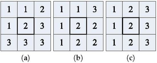
Taking window size of 3 as an example, three typical results of local spatial information classification are explained in the following. As described in Figure 1, the initial label of the pixels is as marked and the central pixel is highlighted with a black box. In accordance with values in Figure 1a, it can be calculated that the label of 3 is the main pixel for this local spatial information block. If the label of 2 is the main misclassified pixel corresponding to label 3, the label of central location is converted to 3 by the proposed SF filter. Otherwise, it will remain unchanged. However, it will be replaced by label of 3 through the proposed MS filter as the further post-processing step. The central pixel of local spatial information similar to the case aforementioned is certain to be reclassified. It is shown in Figure 1b that the main pixel of this local space is 2 or 1. Thus, the filters will not change the value of central location. This situation corresponds to the small misclassified patches within the block. In Figure 1c, it is clear that any of them can be considered as the main pixel in the region, since the number of three labels is the same. In this case, both of the proposed filters have no way to deal with it well. The actual situation corresponding to this instance is quite common in PolSAR image classification, that is, the left side indicates one label, the right side represents another label, and the middle belongs to neither. The middle region is formed by the interaction of two types of categories, so they are labeled as the third kind of label. That is to say, the middle pixels represent the boundary line between two kinds of objects. In fact, the local spatial information of two or more main labels with symmetrical central pixels cannot be well handled.

To summarize, the overall accuracy of classification network based on the proposed MAE with SF filter as post-processing step is bound to increase, while that with MS filter as further post-processing step may not always improve. Although scatter misclassified pixels will not appear and the visual effect of result image will be improved to some extent, MS filter will do damage on some special regions. Besides, two kinds of proposed filters are of little use on the classification of pixels in the misclassified patches and boundaries.

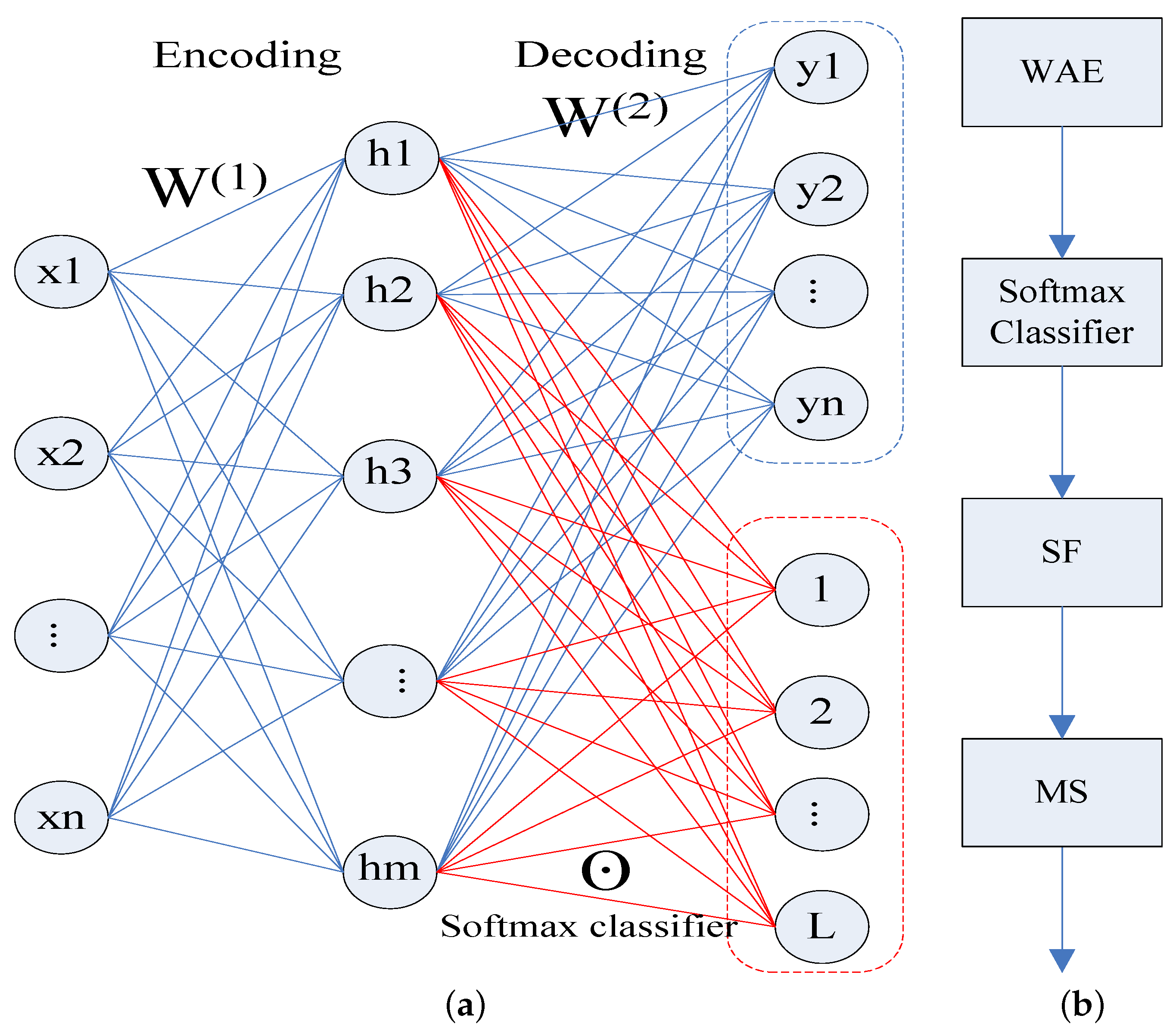
The structure of the proposed WAE is shown in Figure 2a with the blue box, while the classification network, combined with the proposed WAE and Softmax classifier, is given in Figure 2a with the red box. When constructing the loss function of the AE network, the measurement of the data error item is implemented by the Euclidean norm of the errors between the input vector and the reconstructed vector. This is mainly designed for natural images. In addition, it is only applicable to the data that are subjected to Gaussian distribution. For PolSAR images, the original feature of each pixel is expressed only by nine-dimensional information, which is not enough for AE network. At the same time, not all dimensions of the POLSAR data matrix obey the Gaussian distribution. Therefore, in the process of constructing the proposed WAE, we consider not only the distribution of data, but also introduce neighborhood pixels to increase the number of original features.

Auto encoder network is one of unsupervised learning methods, which can automatically learn features from unlabeled data. As a result, 1% of the data, whether labeled or not, is selected to train the proposed MAE in order to obtain the parameters. Then, 5% labeled pixels of each class, randomly selected according to the ground truth image, are used to train the Softmax classifier. Finally, the proposed MAE and Softmax classifier are combined to form a classification network.

In the training process, the input of data is pixel by pixel without considering the spatial position relationship between the pixels. Thus, SF filter is proposed by using the confusion matrix and spatial local information, which designed specifically for the main misclassified pixels. In addition, MS filter is presented for the misclassified scattered points in the result image. Finally, the flow chart of all steps for the proposed classification method is displayed in Figure 2b.

3. Experimental Analysis and Results

In our experiments, three real PolSAR images were selected as the testing images for the proposed classification methods. Test images include Xi’an area, China; Flevoland, The Netherlands; and San Francisco Bay, USA. Three related classification methods, including Wishart classifier, SVM and classification network based on AE, were treated as comparison algorithms of classification network based on the proposed MAE. The results of post-processing steps with two proposed filters on the result images of the four methods are given and compared.

3.1. Introduction of Dataset

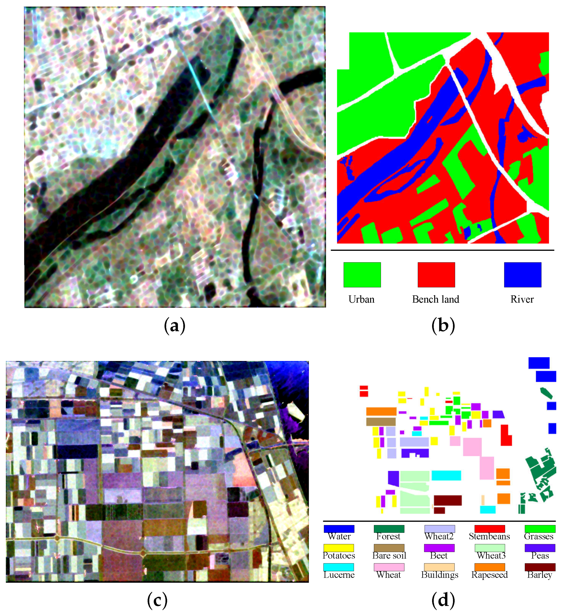
The first dataset covers western Xi’an area, China and was acquired by SIR-C/X-SAR. Its PolSAR image contains a large number of pixels. Only a sub block of size $512\times 512$ was cut out for the experiments. The Pauli RGB image and the corresponding ground truth map are displayed in Figure 3a,b, respectively. There are three classes, including bench land, urban and river. The total number of labeled pixels is 237,416 in the ground-truth map.

The Flevoland image was obtained from a subset of an L-band, multi-look PolSAR data, acquired by the AIR-SAR platform on 16 August 1989, with a size of $750\times 1024$. The Pauli RGB image and the corresponding ground-truth map are shown in Figure 3c,d, respectively. There are fifteen classes in this ground truth, in which each class indicates a type of land cover and is identified by one color. The total number of labeled pixels in the ground truth is 167,712.

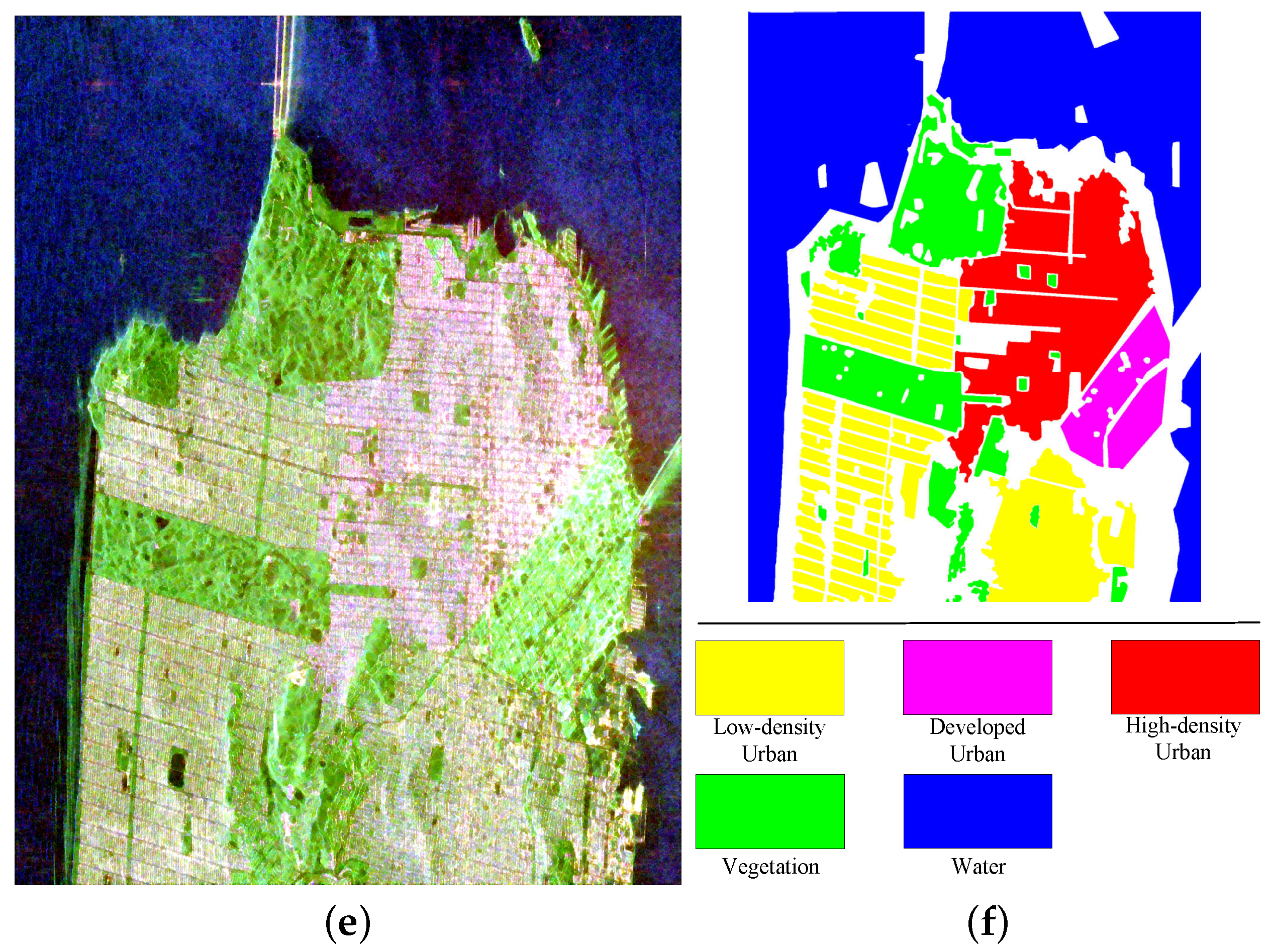
The RADARSAT-2 C-band data of San Francisco Bay was used as the third experimental image. The size of selected scene is $1800\times 1380$ and contains five classes: Water, Vegetation, High-density urban, Low-density urban and Developed urban. The Pauli RGB image and the ground-truth map are shown in Figure 3e,f, respectively. The total number of labeled pixels is 1,804,087.

Finally, the information about these PolSAR images is summarized in

Table 1. Information on Three PolSAR Images.

	Radar	Band	Year	Resolution	Size	Categories
Xi’an area	NASA/JPL SIR-C/X-SAR	C	2010	8 × 8 m	512 × 512 pixels	3
Flevoland	AIRSAR	L	1989	6.6 × 12.1 m	750 × 1024 pixels	15
San Francisco Bay	RADARSAT-2	C	2008	10 × 5 m	1800 × 1380 pixels	5

.

3.2. Selection of Training Sample Rate

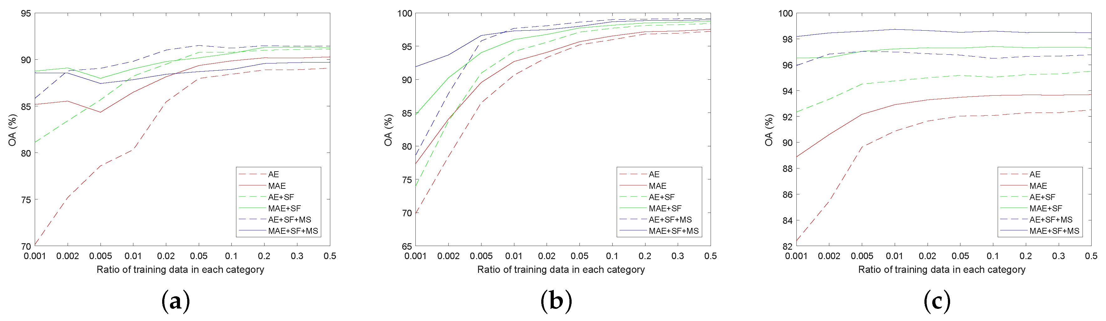
The influence of the ratio of training data on the performance of Softmax classifier based on different AEs for three PolSAR images is discussed. In these experiments, 400 and 0.5 were, respectively, selected as the number of hidden layer nodes and sparsity parameter for the Softmax classifier based on AE and the proposed MAE. Further, 1 × 10${}^{-6}$ and 1 correspond to parameters of the weight decay term and the sparsity penalty term, respectively. For simplicity, the window size of SF filter and MS filter were set to 7.

The overall accuracy (OA) of different ratios of training samples for two classification methods with AE and the proposed MAE feature learning network and that for each of the post-processing steps are shown in Figure 4. Overall accuracy refers to the ratio of the number of pixels being classified correctly to the total number of labeled pixels in the ground truth map. The red, green and blue line in Figure 4 represent the OA of classification method based on features obtained by a specific auto encoder network, OA of post-processing with the proposed SF filter and OA of further post-processing with the proposed MS filter, respectively. Given the same ratio of training samples, the influence of different classification methods on OA is discussed. First, the main misclassified category was determined by analyzing the corresponding confusion matrix, and then the proposed SF filter was used for post-processing. Both jointly led to an inevitable rise in OA (see the relationship between green and red lines in Figure 4 for more details). Similarly, using MS filter on the local spatial information for a further post-processing is only effective for isolated misclassified pixels. Furthermore, pixels near edges and corners can be incorrectly reclassified, resulting in the increase of overall accuracy, which was not as good as that of the classification method with the aforementioned post-processing step. The above-mentioned analytical results could be verified by the relationship of the three lines with different colors shown in Figure 4. Figure 4a shows that the OA obtained by further post-processing step with MS filter was not further improved but decreased. This is because that the MS filter destroyed the classification result of slender rivers in the image. As shown in Figure 4b, the OA of further post-processing step with MS filter increased slightly, compared with the increment of OA obtained by the post-processing step with SF filter. Many symmetric structure boundaries are included in the corresponding ground truth map. MS filter with merely utilizing spatial information also caused misclassified problems for such pixels near the boundaries. As shown by comparing all curves in Figure 4c, the OAs of both classification methods were improved after further post-processing with MS filter. The reason is the ground truth image contains fewer symmetrical structure boundaries and complex and slender structures. Simultaneously, the following conclusion can be drawn from the results in Figure 4: both proposed post-processing methods are suitable for applying to the result image obtained by any classification methods.

From the perspective of the ratio of training data, the following conclusions can also be drawn. While the ratio of training data increased within a certain value, the OAs of both classification methods increased as well. However, when it exceeded that value, the overall accuracy did not increase too much and tended to be stable. By comparing the OA obtained by AE and MAE in different proportions of training data (red lines), the following conclusions can be drawn. The increase of OA was high at the beginning, and then became very small after the ratio of training samples in per category of the three PolSAR images reached 5%, 5% and 0.1%, respectively. To obtain the classification result image of the corresponding truth image more conveniently, all labeled pixels were considered to be the test sample set. The benefit of doing so is that the result image and the correct rate of each category could verify the effectiveness and correctness of the proposed method mutually. Thus, the number of training and testing samples is given in

Table 2. Number of samples for Xi’an image.

Category	Number of Training Samples	Number of Testing Samples
Urban	4197	83,946
Bench land	5889	117,782
River	1784	35,688
Total	11,870	237,416

,

Table 3. Number of samples for Flevoland image.

Category	Number of Training Samples	Number of Testing Samples
Water	662	13232
Stem beans	317	6338
Potatoes	808	16,156
Forest	902	18,044
Grasses	353	7058
Beet	502	10,033
Rapeseed	693	13,863
Peas	479	9582
Lucerne	509	10,181
Bare soil	255	5109
Wheat2	558	11,159
Wheat	819	16,386
Wheat3	1112	22,241
Buildings	37	735
Barely	380	7595
Total	8386	167,712

and

Table 4. Number of samples for San Francisco Bay image.

Category	Number of Training Samples	Number of Testing Samples
Water	852	852,078
Vegetation	237	237,237
High-density urban	283	282,975
Low-density urban	351	351,181
Developed urban	81	80,616
Total	1804	1,804,087

, respectively. The following experiments used this proportion of training data to complete the training of the model.

3.3. Discussion of Parameters

The following tables give the overall accuracy on different combinations of sparsity parameter and the number of hidden nodes by classification networks based on two kinds of AE feature learning.

Table 5. OA on different values of sparsity and number of hidden nodes over Xi’an area image by two classification networks based on AE and the proposed MAE.

	300	400	500	600	700	800	900
0.01	0.7694	0.7731	0.7940	0.7902	0.7912	0.8018	0.8094
	0.8940	0.8914	0.8935	0.8951	0.8953	0.8959	0.8964
0.05	0.8158	0.8213	0.8381	0.8371	0.8385	0.8413	0.8433
	0.8943	0.8939	0.8937	0.8962	0.8942	0.9003	0.8998
0.10	0.8273	0.8410	0.8496	0.8528	0.8546	0.8553	0.8559
	0.8968	0.8946	0.8945	0.8959	0.8961	0.8977	0.8966
0.50	0.8759	0.8777	0.8802	0.8779	0.8780	0.8749	0.8720
	0.8951	0.8941	0.8934	0.8934	0.8940	0.8946	0.8950
1.00	0.8825	0.8863	0.8860	0.8862	0.8881	0.8880	0.8885
	0.8954	0.8943	0.8948	0.8939	0.8941	0.8944	0.8953

,

Table 6. OA on different values of sparsity and number of hidden nodes over Flevoland image by two classification networks based on AE and the proposed MAE.

	300	400	500	600	700	800	900
0.01	0.9013	0.9148	0.9252	0.9298	0.9374	0.8703	0.9015
	0.9505	0.9495	0.9502	0.9377	0.9411	0.9366	0.9383
0.05	0.9421	0.9489	0.9516	0.9531	0.9554	0.9555	0.9556
	0.9537	0.9531	0.9542	0.9548	0.9559	0.9582	0.9558
0.10	0.9481	0.9515	0.9553	0.9557	0.9572	0.9571	0.9589
	0.9534	0.9560	0.9549	0.9561	0.9560	0.9585	0.9572
0.50	0.9502	0.9502	0.9531	0.9510	0.9512	0.9504	0.9514
	0.9561	0.9568	0.9563	0.9572	0.9578	0.9574	0.9599
1.00	0.9355	0.9355	0.9350	0.9316	0.9286	0.9311	0.9262
	0.9562	0.9567	0.9578	0.9581	0.9575	0.9579	0.9605

and

Table 7. OA on different values of sparsity and number of hidden nodes over San Francisco Bay image by two classification networks based on AE and the proposed MAE.

	300	400	500	600	700	800	900
0.01	0.6862	0.7146	0.7222	0.7294	0.7404	0.7456	0.7650
	0.8930	0.8897	0.8883	0.8906	0.8890	0.8891	0.8884
0.05	0.8024	0.8110	0.8140	0.8258	0.8222	0.8329	0.8345
	0.8910	0.8914	0.8890	0.8895	0.8893	0.8879	0.8869
0.10	0.8020	0.8073	0.8222	0.8161	0.8168	0.8254	0.8275
	0.8871	0.8885	0.8891	0.8886	0.8886	0.8899	0.8874
0.50	0.8279	0.8218	0.8259	0.8256	0.8257	0.8309	0.8265
	0.8890	0.8905	0.8885	0.8881	0.8866	0.8874	0.8882
1.00	0.8310	0.8365	0.7378	0.8381	0.8366	0.8367	0.8373
	0.8890	0.8874	0.8876	0.8899	0.8888	0.8884	0.8882

correspond to the results of three PolSAR images, namely Xi’an area, Flevoland and San Francisco Bay, respectively. The upper one of each cell in the three tables represents the overall accuracy of classification network based on AE under a specific combination of parameters, while the other indicates the OA of classification network based on the proposed MAE.

Each column in the tables shows the impact of different sparsity parameters on the OA of two classification networks based on a specific AE structure. Sparsity parameter is the proportion of features that used to train the classifier after feature learning from original data with auto encoder process. Compared with classification network based on the proposed MAE, the OA of classification network based on AE has a greater dependence on sparsity parameter. The larger sparsity parameter for AE network is, the higher classification accuracy will be. However, the OA of classification network based on the proposed MAE has a better robustness to the selection of sparsity parameter. Similarly, it could be concluded from each row of the tables that the number of hidden nodes had a similar effect on the classification accuracy of the AE algorithm, when sparsity parameter was fixed. With the increasing of the number of hidden nodes, the OA of AE classification method increased and then tended to be stable, while the OA of classification network based on the proposed MAE almost kept unchanged. The last row represents directly mapping data to high-dimensional feature space without using sparse constraint item.

Two parameters together determine the number of features used for classifier. Obviously, it is necessary to find a suitable combination of parameters for AE method in order to achieve a better classification effect. If the number of features is small, characteristics of the data cannot be fully expressed, which leads to an unsatisfactory classification accuracy. On the contrary, this number should be as small as possible. With further increasing of network structure, the improvement of classification overall accuracy will not be too large. Inversely, it will cause the increase of network parameters that need to be learned. However, from the corresponding OA value it can be concluded that the proposed MAE relies less on these two parameters, which shows the extracted features have a widely representative. Overall, the proposed MAE is much more robust to the selection of parameters in comparison with the AE network. Both the smaller sparsity parameter and the larger number of hidden layer nodes cannot make the two classification networks obtain good results at the same time. Hence, a suitable combination of parameters should be selected to complete the following experiments for each PolSAR image.

3.4. Result and Analysis

3.4.1. Xi’an Area Image

According to the analysis of selection of parameters, we selected 300 as the number of nodes in hidden layer and applied 0.05 as sparsity parameter in this experiment. Then, 1 × 10${}^{-6}$ and 1 were chosen as the weight of weight decay term and sparsity penalty term, respectively. Here, we discuss the classification result on Xi’an area image of different methods, including Wishart classifier, SVM, classification network based on AE, classification network based on the proposed MAE and their post-processing (PP) step, respectively. The correct rate of each category and overall accuracy for the four comparison methods and the corresponding PP steps are listed in

Table 8. The correct rate of each category and overall accuracy for the four comparison methods and those of the corresponding PP steps for Xi’an area image.

	Urban	Bench Land	River	OA
Wishart	0.8241	0.8322	0.9393	0.8454
SVM	0.9034	0.9258	0.8921	0.9128
AE	0.7694	0.8204	0.8727	0.8102
MAE	0.8816	0.9094	0.8996	0.8981
Wishart+PP	0.8692	0.8584	0.9459	0.8754
SVM+PP	0.9277	0.9441	0.8874	0.9298
AE+PP	0.8732	0.9010	0.9167	0.8935
MAE+PP	0.9110	0.9322	0.9030	0.9203

and the maximum value of them among the four methods is expressed in bold.

According to the data in Table 8, we can draw the following conclusions. For Urban and Bench land, the correct rate of SVM is over 90%, which is the highest among the four comparison methods without any post-processing step. However, the correct rate of Wishart classifier for River is the best and up to 93%. Simultaneously, the correct rate of Wishart classifier for other kinds of categories is nearly 83%, which leads to its overall accuracy being not as good. Compared with the classifier based on AE, the correct rate of each category for classifier network based on the proposed MAE has a great increase. Therefore, the proposed MAE has a better ability to represent the characteristics of PolSAR data. Although the accuracy of SVM for River is lower than that of Wishart classifier and classifier based on the proposed MAE, the OA of SVM is still the highest. This is because the total number of pixels in River is far less than that of other categories. The proposed classification method follows closely. The difference between them is less than 2% in OA. The post-processing step with SF filter is carried out under the qualitative analysis of confusion matrix, so the accuracy after processed by SF filter is bound to increase. Owing to the ground-truth image of Xi’an area containing relatively slender regions, MS filter merely using spatial location information will inevitably cause damage to the original classification results and reduce the correct rate of a certain category. These points were verified in the analysis presented in the previous section. In this case, further post-processing step with utilizing MS filter reduced the correct rate of River. Due to the limitation of space, we directly give the result processed by both of the proposed filters. It can also be seen in Table 8 that the classification overall accuracy of all the methods was improved to a certain extent after the post-processing step. Thus, the validity of post-processing steps with using the proposed SF and MS filter was verified again.

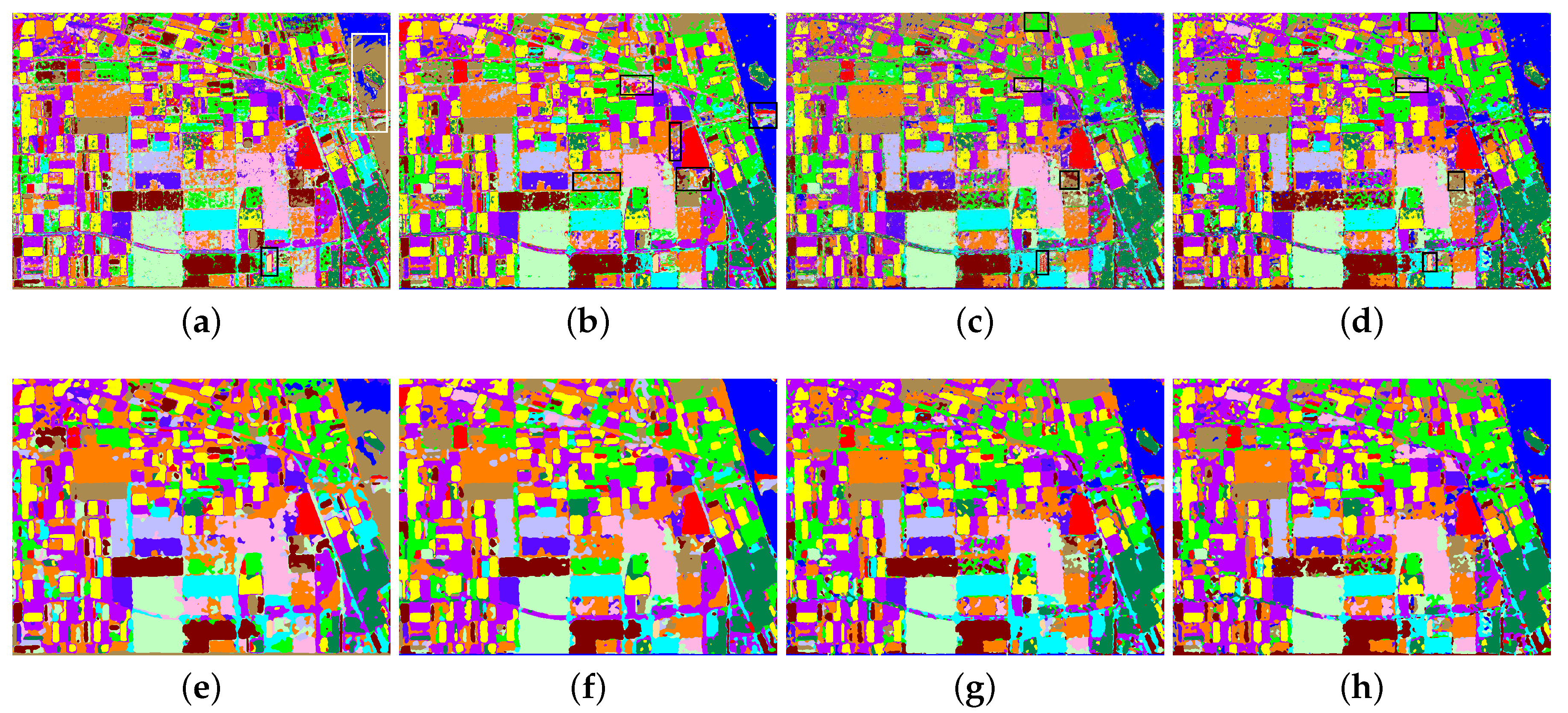
Figure 5 shows the classification result image corresponding to the ground-truth of Xi’an area obtained by different methods. The classification result of Wishart classifier is given in Figure 5a. Black rectangle is used to highlight the notable misclassified areas, in which a large number of misclassified small patches appear. The visual effect of the result image is unsatisfactory. The classification result image of SVM is displayed in Figure 5b. It can be seen that SVM achieved a better classification effect on three kinds of categories, compared with the ground truth image. Figure 5c represents the result image obtained by the classification network based on AE. It can be concluded that there are a lot of pixels in the image that are not classified correctly, which leads to noise appearance in the overall visual effect of the image. However, this situation is suppressed to some extent in the result image of our proposed method, as shown in Figure 5d. Clearly, the comparison of Figure 5c,d shows the correctness of introducing data distribution into the design of auto encoder network. The result images of four comparison methods with the proposed SF and MS filter as post-processing steps are given in Figure 5e–h, respectively. The main misclassified scatter pixels of each class in the result images are reclassified. Each pixel block in the image is smoother. As a whole, the visual effect is improved as well. However, it should be pointed out that, among all the methods, classification performance of Wishart classifier is the best for pixels of River, shown with the white rectangle. Moreover, the post-processing steps destroy the classification of the slender areas, e.g., the black ellipse regions.

3.4.2. Flevoland Image

In this experiment, the number of nodes in hidden layer and sparsity parameter were chosen as 400 and 0.1, respectively. The correct rate of each class and overall accuracy are listed in

Table 9. The correct rate of each category and overall accuracy for the four comparison methods and those of the corresponding PP steps for FLEVOLAND image.

	Water	Stem Beans	Potatoes	Forest	Grasses	Beet	Rapeseed	Peas
Wishart	0.5008	0.9262	0.8727	0.8728	0.6849	0.9178	0.7398	0.9416
SVM	0.9983	0.9946	0.9585	0.9650	0.9498	0.9940	0.9299	0.9858
AE	0.9880	0.9571	0.9332	0.9367	0.9320	0.9765	0.9144	0.9231
MAE	0.9958	0.9864	0.9353	0.9489	0.9467	0.9740	0.9157	0.9675
Wishart+PP	0.5344	0.9921	0.9790	0.9174	0.7526	0.9829	0.7933	0.9898
SVM+PP	1.0000	0.9953	0.9967	0.9905	0.9908	0.9969	0.9857	0.9960
AE+PP	0.9979	0.9964	0.9931	0.9768	0.9708	0.9927	0.9840	0.9758
MAE+PP	1.0000	0.9972	0.9924	0.9794	0.9770	0.9979	0.9771	0.9947
	Lucerne	Bare soil	Wheat2	Wheat	Wheat3	Buildings	Barley	OA
Wishart	0.7695	0.9883	0.8060	0.8672	0.8845	0.8204	0.9485	0.8302
SVM	0.9774	0.9978	0.9060	0.9612	0.9874	0.8980	0.9875	0.9686
AE	0.9754	0.9843	0.9103	0.9449	0.9789	0.3973	0.9862	0.9491
MAE	0.9740	0.9885	0.8911	0.9589	0.9773	0.7061	0.9863	0.9567
Wishart+PP	0.7777	0.9975	0.9338	0.9140	0.9518	0.8136	0.9609	0.8876
SVM+PP	0.9894	1.0000	0.9678	0.9874	0.9949	0.8163	0.9993	0.9910
AE+PP	0.9845	0.9992	0.9772	0.9812	0.9891	0.5102	0.9989	0.9842
MAE+PP	0.9889	0.9994	0.9632	0.9812	0.9880	0.7605	0.9978	0.9859

. The maximum value of each of them is marked in bold. For Wishart classifier, the correct rate of Water, Grasses, Rapeseed and Lucerne was less than 80%, while that of the rest exceeded 80%. The accuracy of Water was as low as 50%, which is unacceptable. In other words, the OA of Wishart classifier was merely 83%, which is not a satisfactory result. SVM had a better classification ability of all categories, the OA of which was up to 96.8%. For most categories, the correct rate of SVM was more than 90%. It should be pointed out that both of the supervised classification methods, namely Wishart classifier and SVM, had a better result for Buildings in comparison with the classification networks based on different AEs. The reason is that the number of pixels in Buildings is relatively small, which is not enough for the training process of classification networks. For Stem bean, Peas, Wheat and Buildings, the correct rate of classification network based on the proposed MAE was far higher than that of classification network based on AE. With regard to the remaining categories, there was not much difference between the two classification networks on OA. In particular, the accuracy of Buildings by classification network based on AE was as low as 40%, which is very unsatisfactory, while that by classification network based on the proposed MAE reached 70%. The OA of classification network based on the proposed MAE was more than 95%, about 1% higher than that of classification network based on AE.

After post-processing step with both of the proposed filters, the correct rate of Potatoes, Rapeseed, Wheat2 and Buildings were about 5% higher than that of classification network based on the proposed MAE. For the remaining categories, the improvement of accuracy was less than that of the previous categories, ranging from two thousandths to a few percent. In terms of overall accuracy, it was up to 98.6%. The correct rate of the vast majority of categories was close to or greater than 97% by introducing two proposed filters with local spatial information as post-processing steps. As shown in Table 9, similar conclusions can be obtained from the comparison of the results on correct rate of each category obtained by classification network based on AE and those of its post-processing steps. Except for pixels of Buildings, the use of two filters to process the classification results of SVM and Wishart classifiers could improve the correct rate of most categories. As with the aforementioned image, the overall accuracy of SVM with post-processing steps increased to 99%, which was the highest among the four comparison methods. Nevertheless, the OA of the proposed method ranked second with a gap of 0.005. Moreover, the OA of classification network based on AE fell behind slightly. The OA of Wishart classifier after post-processing by two filters was the lowest and nearly 89%. To sum up, the post-processing steps with utilizing two proposed filters are suitable for these methods.

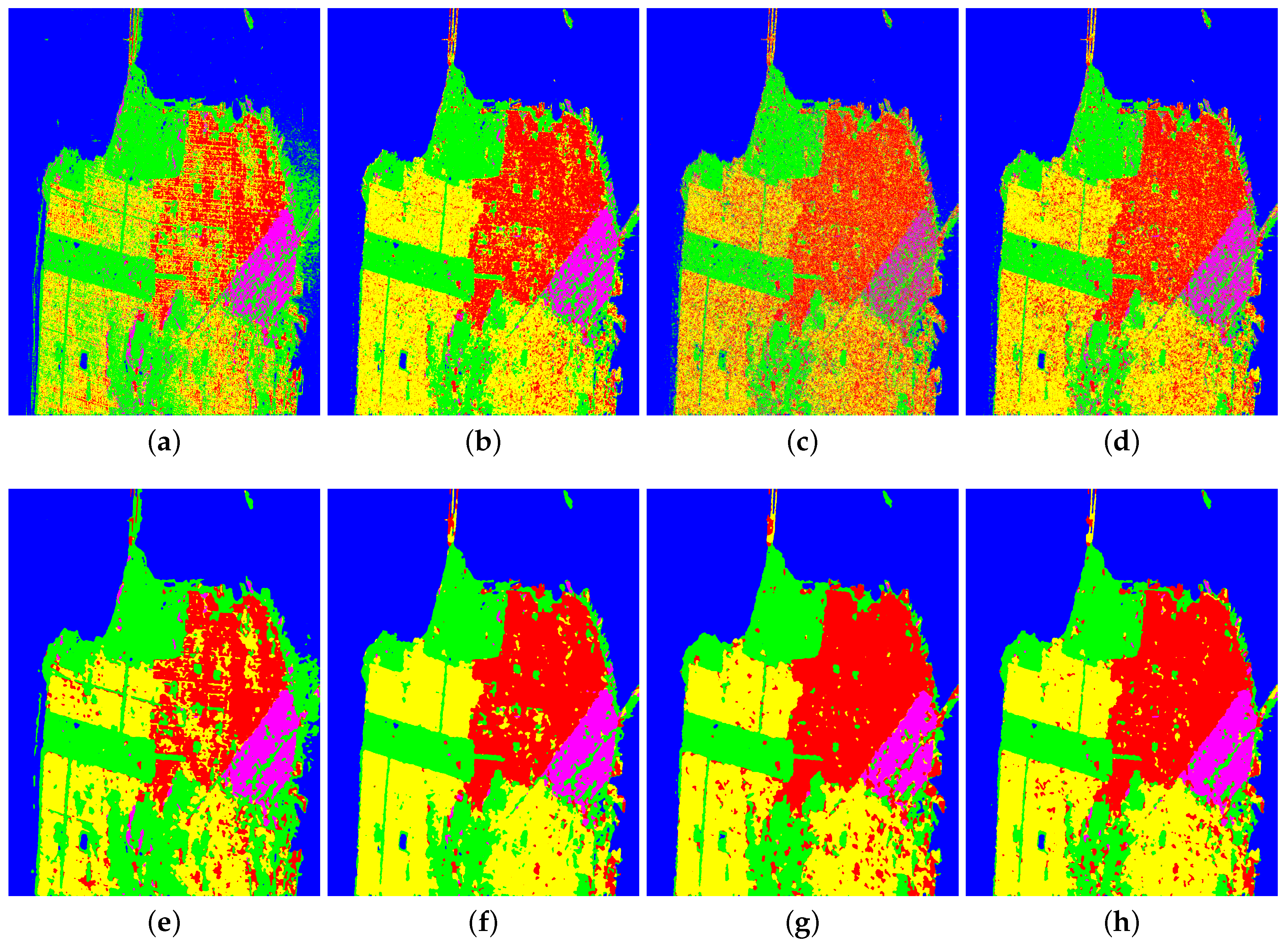
Then, the prediction result for all the pixels in the image of the eight classification methods are shown in Figure 6. For each block in the result image of Figure 6a, there are always some pixels being misclassified. In particular, most of the Water pixels are divided into pixels of Bare soil, as highlighted with a white rectangle. Nevertheless, Wishart classifier can properly classify most of the pixels of Buildings, as shown with a black rectangle. The above analysis indicates that the quantity of training data in each category affects the classification performance of Wishart classifier for each category. It is noticeable that more training data have an opposite influence on the classification accuracy of Wishart classifier. From the result image in Figure 6b, it can be obtained that SVM has a strong ability to predict the label of pixels. The overall classification effect of the result image is good. As shown in black rectangles, it was found that several blocks of pixels are poorly classified after making a comparison with the ground truth image. Compared with Figure 6c,d, classification networks based on AE and the proposed MAE can generally predict the labels of each block better. Both possess the corresponding regions with good classification effect and produce some erroneous classified pixels simultaneously. Including Buildings, the classification effect on most categories with classification network based on the proposed MAE was better than that of classification network based on AE. For regions shown in a black square box, the visual effect of classification network based on the proposed MAE was better than those of the classification network based on AE. The result image after post-processing with the proposed filters by four methods is given in Figure 6e–h, respectively. Overall, the visual effect of post-processing result images was better than that of the result images obtained by each method, and mistakenly classified scattered points vanished. However, there are still some small patches of incorrectly classified pixels clustered together by making a careful comparison with the ground truth image. Further, it is worth pointing out that the pixels near the boundary between the two category have not been well handled due to the inadequacy designing of the proposed filters. Once the classification of boundary pixels is inaccurate, this trend will spread to the surrounding pixels. A similar over-segmentation is caused at the boundaries of blocks in the image. In conclusion, the predicted images shown in Figure 6 validate the performance of classification network based on the proposed MAE and the rationality of the analysis about two post-processing steps once more.

3.4.3. San Francisco Bay Image

According to the analysis of selection of parameters, we selected 500 as the number of nodes in hidden layer and applied 0.5 as sparsity parameter in this experiment. The correct rate of each class and overall accuracy are listed in

Table 10. The correct rate of each category and overall accuracy for the four comparison methods and those of the corresponding PP steps for SAN FRANCISCO BAY image.

	Water	Vegetation	High-Density Urban	Low-Density Urban	Developed Urban	OA
Wishart	0.9712	0.9230	0.5231	0.6853	0.6485	0.8245
SVM	1.0000	0.9289	0.8083	0.8420	0.7349	0.9180
AE	0.9996	0.8342	0.6746	0.6160	0.4495	0.8276
MAE	0.9999	0.8833	0.7773	0.7612	0.6649	0.8882
Wishart+PP	0.9832	0.9715	0.6950	0.7849	0.7728	0.8884
SVM+PP	1.0000	0.9649	0.9382	0.9346	0.8401	0.9662
AE+PP	1.0000	0.9610	0.9795	0.8443	0.7221	0.9489
MAE+PP	1.0000	0.9564	0.9699	0.9179	0.8538	0.9670

. The maximum value of each of them is marked in bold.

The following conclusions are drawn from the data in Table 10. For the category of Water, correct rate of all the other classification methods could reach more than 99%, except for Wishart classifier. Moreover, the accuracy of Water obtained by SVM was up to 100%, which was the best classification performance on the pixels of Water among four methods. For the pixels of Vegetation, the correct rate of classification network based on the proposed MAE was about 5% higher than that of classification network based on AE. The correct rate of two supervised classification methods, namely Wishart classifier and SVM, was more than 92%, which was greater than that of classification network based on MAE. For Wishart classifier, the correct rate of three kinds of urban areas was less than 70%. Especially, the classification accuracy of Wishart classifier for High-density urban was only 52%, which is a very unsatisfactory result. Moreover, the correct rate of classification network based on AE for the rest categories was almost the worst among all the methods. Particularly, the correct rate of Developed urban was only about 45% and much lower than that of the classification network based on the proposed MAE. This shows that the proposed MAE with the consideration of different distributions of PolSAR data matrix has a better ability of feature extraction. For three kinds of urban categories, the classification network based on the proposed MAE was always higher than that of classification network based on AE. In addition, the classification accuracy of SVM for the rest categories of urban areas was more than 73%, which was the best among the first four classification methods. The lowest classification accuracy rate of them was Developed urban area, which was 7% higher than that of classification network based on the proposed MAE. The reason for obtaining relative low correct rate of three urban regions by two classification networks may be that one thousandth of training data was insufficient for the parameters of network structure that needed to be trained. However, more importantly, the correct rate of each category was greatly improved after utilizing post-processing steps with two proposed filters. Besides, the correct of each category was also higher than that of each without any processing, after the post processing steps were performed on the result images of Wishart classifier and SVM. The above-mentioned shows that the proposed filters have better ability to improve the result of classification and universal applicability.

We can also make the following conclusions from the prediction result images shown in Figure 7. The result images of all the classification methods have a good classification performance on the pixels of Water, except that of Wishart classifier. From the middle part of the right side of the result image shown in Figure 7a, it is known that the pixels of Water is classified as those of Vegetation in error. However, the corresponding regions of other resulting images are well handled. For the main regions of Vegetation, the classification effect of Wishart classifier and SVM looks much smoother than those of two classification networks based on different AEs, in which most of the Vegetation pixels are misclassified into those of High-density urban. For the three kinds of urban areas, the visual effect of Wishart classifier and classification network based on AE is obviously not as good as that of other classification methods. As shown in Figure 7b, the performance of SVM for these urban areas is definitely superior to that of classification network with AE and the proposed MAE. According to the comparison of Figure 7c,d, it can be seen that High-density urban and Low-density urban are the main misclassified pixel of the other party, respectively. Meanwhile, there is no doubt that the number of misclassified pixels by the classification network based on the proposed MAE is less than that of the classification network based on AE. For the areas of High-density urban and Developed urban, it is difficult to judge which is the best only by observing the pixels in the result images of SVM and that of the proposed method. The result images obtained by using the post-processing steps on the result images of different classification methods is shown in Figure 7e–h, respectively. From the comparison of the result image and the result image after postprocessing with two proposed filters obtained by each classification method, we can draw the following conclusions. The scattered pixels of other categories within each block in the result image after postprocessing are well reclassified, which makes the result images smoother and cleaner. However, there are still some small patches, in which the misclassified pixels centralized in the result image and were not well classified. That is, neither filters has a better ability to process regions centralized with misclassified pixels. The reason for this is that the designing of the proposed filters does not fully consider the case of multiple optimal values of pixels in a local area. From the overall classification effect, the result images of SVM and the proposed MAE are better than that of the other two methods. In summary, the validity of classification network based on the proposed MAE and the correctness of two post-processing steps with utilizing spatial information are proved. Moreover, the observation confirms the results of previous analysis on objective indexes once more.

Finally, we analyzed the execution efficiency of the classification methods from the point of view of time. The training time of three PolSAR images with different methods is given in

Table 11. Training time of three PolSAR images with different methods (s).

	Xi’an Area	Flevoland	San Francisco Bay
Wishart	0	0	0
SVM	2677.90	1719.51	1493.18
AE	103.67	280.10	471.81
MAE	25.24	135.33	138.98

. Wishart classifier directly selects some labeled data to compute the initial classification center in order to finish the supervised classification. Thus, the training time is considered to be zero. In the experiments, the LIBSVM was selected as the implementation of SVM. Moreover, it is necessary to find the optimal combination of parameters within a certain range. For three PolSAR images, it took more than 1000 s to accomplish the training process of SVM, including that of the optimization of parameters. It took more than 100 s to complete the training process of classification network based on AE for three PolSAR images. However, the training time required for the proposed MAE with same classification process was one fourth to a half of that. The two post-processing steps with filters are based on spatial local information. The only thing needed to be done is giving values of the corresponding parameters. It is supposed to not consume the training time. To save space, we do not show the training time of post-processing in the table. In fact, the training time is affected by many factors, such as the number of training sets, the number of parameters contained in the structure of network being trained, the scope of parameter optimization and the number of iterations. Although SVM achieved a better classification overall accuracy for four comparison methods, using a classifier with AE neural network greatly saved training time, on the premise that the classification overall accuracy was not too bad.

Table 12. Predicting time for all pixels in three PolSAR images with different methods (s).

	Xi’an Area	Flevoland	San Francisco Bay
Wishart	13.4	194.73	198.83
SVM	345.55	700.62	552.45
AE	45.47	161.56	638.70
MAE	43.08	160.56	622.82
Wishart+PP	4.53	25.28	45.19
SVM+PP	4.16	26.15	46.27
AE+PP	3.97	24.84	42.79
MAE+PP	3.91	24.09	64.38

shows the time for predicting the label of all pixels in three PolSAR images with different methods. Among the four comparison methods, the predicting time of Wishart classifier was the least for each of the PolSAR image. The process of predicting the pixels of the PolSAR image with SVM cost a lot of time. For classification networks based on two different feature extraction methods, their predicting time was not much different. In addition, all of the methods spent several to tens of seconds of extra time to complete the post-processing steps to get the predicting label of all pixels. In brief, it is reasonable and worthwhile to spend tens of seconds in exchange for a greater improvement in the overall accuracy. Finally, it should be pointed out that this time is mainly proportional to the number of pixels to be predicted.

3.5. Illustration to Post-Processing Steps

Table 13. Confusion matrix of labeled pixels obtained by classification network based on the proposed MAE.

	Urban	Bench Land	River
Urban	0.8816	0.1141	0.0043
Bench land	0.0546	0.9094	0.0359
River	0.0034	0.0970	0.8996

shows confusion matrix of the labeled pixels in the Xi’an area image, obtained by classification network based on the proposed MAE. The main misclassified category for each category are show in Table 13. For example, the main misclassified category of Urban is Bench land. The core of the proposed SF filter is that if the main misclassified pixel is surrounded by pixels of main category, it should be changed into the pixel of main category. 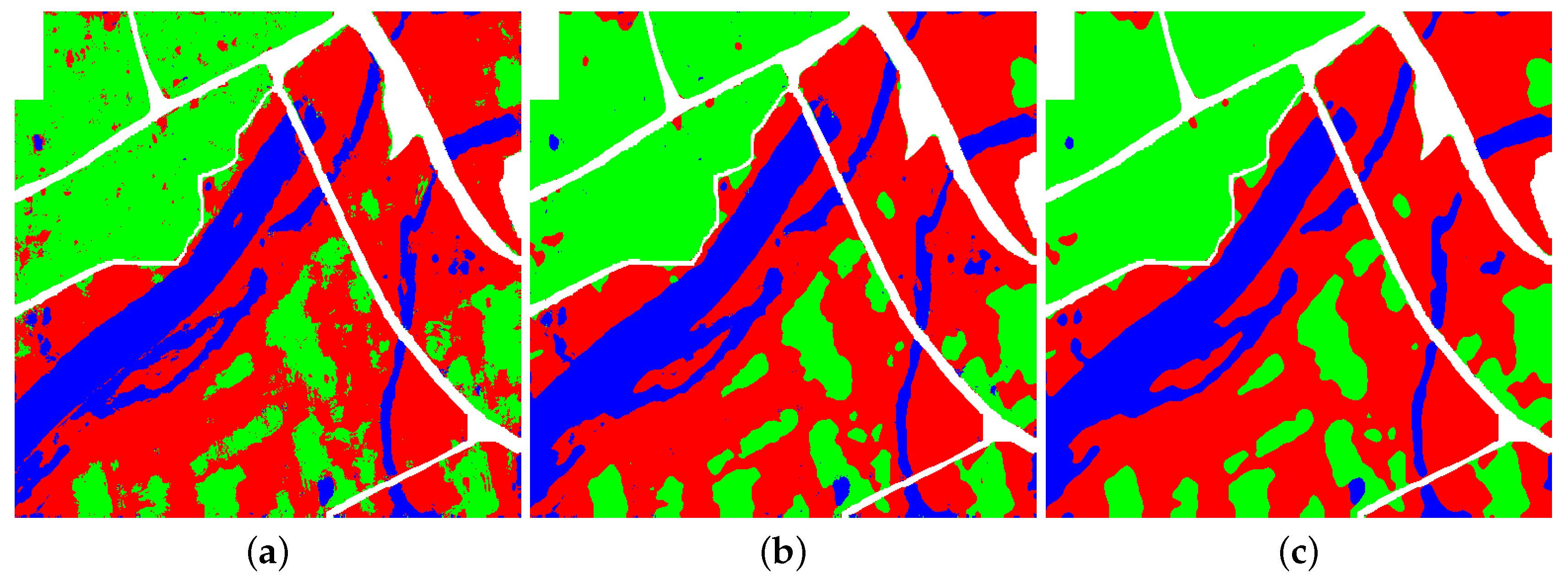Figure 8 shows the classification result image of the proposed MAE and the result images after each post-processing step, respectively. From the result image in Figure 8a,b, scatter points of Bench land in the former was indeed replaced by the main category pixel of Urban shown in the latter one. To other categories, a consistent conclusion can be drawn from the relationship of confusion matrix and the corresponding result image.

Nevertheless, the proposed SF filter also has some shortcomings. It does not have a good inhibitory effect on patches formed by wrong classification points. Apparently, SF filter does not take any measures to deal with categories of other misclassified pixels as well. From the confusion matrix, it can be concluded that the number of other misclassified pixels is very small. Hence, the further post-processing step, completed by the proposed MS filter, merely uses spatial location information to process the isolated misclassified pixels, which makes the result image shown in Figure 8c smoother and have better visual effect. However, there still exists some problems in this experiment. Corners and sharp edges in the original image were wrongly classified. Compared the corresponding ground-truth image, it can be seen that pixels in the narrow area of River were classified as Urban by error. This phenomenon can be lightened by reducing the size of the filter window. Therefore, the correctness of analysis shown in Figure 5 was verified once more.

4. Conclusions

In this paper, based on the distribution of different rows in PolSAR data matrix, a mixture auto encoder network is proposed for features learning and a classification network is given through connecting with a Softmax classifier as well. To improve the classification effect better, not only the distribution of PolSAR data matrix but also the neighborhood information is considered into the proposed method of features learning. In addition, a SF filter is proposed to deal with the inevitably misclassified pixels in the block of pixels. It is designed specifically for the main misclassified pixels. At the same time, this paper also presents a MS filter to process pixels of other misclassified categories. Both filters are used as post-processing steps to deal with the result image of our proposed classification network, which improve the visual effect of the PolSAR classification image and increase the overall accuracy in a certain extent. Future work includes providing more rigorous proof for the distribution of the PolSAR data matrix and further improving the theoretical process of the proposed feature extraction method. Meanwhile, the application of multi-layer classification network is also one of the main tasks.