Ensemble-Based Cascaded Constrained Energy Minimization for Hyperspectral Target Detection

Abstract

Ensemble learning is an important group of machine learning techniques that aim to enhance the nonlinearity and generalization ability of a learning system by aggregating multiple learners. We found that ensemble techniques show great potential for improving the performance of traditional hyperspectral target detection algorithms, while at present, there are few previous works have been done on this topic. To this end, we propose an Ensemble based Constrained Energy Minimization (E-CEM) detector for hyperspectral image target detection. Classical hyperspectral image target detection algorithms like Constrained Energy Minimization (CEM), matched filter (MF) and adaptive coherence/cosine estimator (ACE) are usually designed based on constrained least square regression methods or hypothesis testing methods with Gaussian distribution assumption. However, remote sensing hyperspectral data captured in a real-world environment usually shows strong nonlinearity and non-Gaussianity, which will lead to performance degradation of these classical detection algorithms. Although some hierarchical detection models are able to learn strong nonlinear discrimination of spectral data, due to the spectrum changes, these models usually suffer from the instability in detection tasks. The proposed E-CEM is designed based on the classical CEM detection algorithm. To improve both of the detection nonlinearity and generalization ability, the strategies of “cascaded detection”, “random averaging” and “multi-scale scanning” are specifically designed. Experiments on one synthetic hyperspectral image and two real hyperspectral images demonstrate the effectiveness of our method. E-CEM outperforms the traditional CEM detector and other state-of-the-art detection algorithms. Our code will be made publicly available.

1. Introduction

Hyperspectral remote sensing measures the reflectance from the earth’s surface materials at hundreds of narrow and contiguous wavelength bands. A hyperspectral image captured by an imaging spectrometer can be considered as a three-dimensional data called “data cube” with two spatial dimensions and one spectral dimension. Since each hyperspectral pixel contains a large number of bands with corresponding wave reflectance, its spectral characteristics can be applied to distinguish different materials [1,2].

In recent years, hyperspectral image target detection has become a research hot spot in the image processing field and it has wide applications, both in military and civilian fields. Hyperspectral image target detection is of great significance for military reconnaissance and strike. It can be used to detect important military targets [3,4], such as aircraft, ships, airports, oil tanks, etc. In the field of ecology and forest science, hyperspectral image target detection can be used to detect newly grown leaves [5]. In the field mineral prospecting, hyperspectral image target detection can be used to detect iron oxides [6]. In other civilian fields, it also has a great number of applications such as post-disaster rescue [7] and gas-detection [1]. Many hyperspectral image target detection algorithms have been proposed. Spectral angle mapper (SAM) [8] and Spectral Information Divergence (SID) [9] are two very simple and straightforward detection algorithm which measures the “distance” between the spectrum of the test pixel and the prior spectral signature of the target. The adaptive coherence/cosine estimator (ACE) [10,11], the matched filter (MF) [11], and Matched Subspace Detectors (MSD) [12] are hypothesis-test-based detection algorithms based on Gaussian distribution assumption of the spectral data and is derived from generalized likelihood ratio (GLR) test. The Constrained Energy Minimization (CEM) [2,10] detection algorithm builds a linear filter that minimizes the total spectral output energy under the constraint that the target’s output is a constant. On the basis of these algorithms, some of their recent improved versions have been proposed, such as Matched Shrunken Subspace Detectors (MSSD) [13], the robust CEM detector [14], the Total Variation Detector (TVD) [15] and Robust High-Order Matched Filter (RHMF) [16], Hierarchical CEM detector (HCEM) [17], etc. Some subspace based hyperspectral image target detection algorithms have also been proposed, such as the Orthogonal Subspace Projection (OSP) [18,19] and the Adaptive Subspace Detector (ASD) [20]. OSP projects pixel vectors into orthogonal subspaces of undesired spectral signatures to reduce the data dimensionality and suppress the interference of undesired signatures. ASD originates from the problem of binary hypothesis testing. OSP and ASD require prior knowledge of target spectral features and background spectral features, while a complete statistical characteristic of background spectral features is difficult to obtain in real-world applications. In addition to the subspace based algorithms, some other non-Gaussian based hyperspectral image target detection algorithms have also been proposed, such as elliptically contoured distributions based algorithms [21], Gauss-Markov random field (GMRF) based algorithms [22,23], sparse representation based algorithms [24,25] and non-parametric approaches based algorithms [26].

In recent years, deep learning technology [27,28,29] has made great breakthroughs in computer vision and remote sensing field, such as target detection [30,31,32], image segmentation [33,34], image captioning [35,36], etc. By building cascaded structures and using nonlinear functions, such as ReLU and sigmoid functions, a deep learning model obtains strong nonlinearity which learns high-level abstraction of the input data layer by layer. It is worth noting that the nonlinear function is important for the model to obtain the strong nonlinearity. If only the cascade structures are used without any nonlinear function, the model will still be linear. Since hyperspectral data captured in real environment usually shows strong nonlinearity and non-Gaussianity due to the influence of imaging noise, atmospheric turbulence, and spectral-mixing [17], similar ideas have been brought to hyperspectral target detection and some cascaded detection algorithms have been proposed recently, such as iteratively Reweighted ACE detector (RACE) [37], Hierarchical CEM detector (HCEM) [17], etc. However, these algorithms usually show instability since the inherent variability in target spectral signatures [15] sometimes leads to an overfitting problem when building nonlinear or hierarchical detectors based on biased spectral data.

The nonlinear discrimination ability and generalization ability are both important factors for any machine learning models as well as for any hyperspectral target detection algorithms. It is important to make a trade-off between the two properties when designing a hyperspectral image target detection algorithm. On one hand, the classical detection algorithms, such as CEM, MF, and ACE, have strong generalization ability but weak discrimination ability. These algorithms are not suitable to apply to detection problems with strong nonlinear distribution of spectral data. On the other hand, the hierarchical detection algorithms have strong discrimination ability but weak stability.

Ensemble learning is a group of important machine learning techniques which aims to enhance the nonlinearity and generalization ability of a learning system by aggregating the training and prediction of multiple learners [38,39,40,41]. Ensemble learning methods can be roughly divided into two sub-groups, (1) boosting based methods and (2) bagging based methods, where the former one constructs cascaded learners that are associated with each other during training and prediction [39,42,43] while the latter one constructs independent learners in parallel [40,41].

Considering the above problems, by incorporating the idea of ensemble learning, we propose a new hyperspectral image target detection algorithm called Ensemble based Constrained Energy Minimization (E-CEM) for hyperspectral target detection. In E-CEM algorithm, three strategies are specifically designed to improve both of its nonlinear discrimination and generalization ability, (1) cascaded detection, (2) random averaging and (3) multi-scale scanning.

• Cascaded Detection

Firstly, we use the strategy, “cascaded detection”, to improve the nonlinear discrimination ability. Traditional hyperspectral image target detection algorithms usually follow a detection paradigm of “single layer detection” or “one-time detection”. Inspired by the idea of cascaded operation in boosting algorithms, we propose a cascaded detection structure. In the framework of cascade structure, the sigmoid nonlinear function is used between layers to transform the output of each layer in nonlinear to improve the nonlinear performance of the detector.

• Random Averaging

Secondly, we use the strategy, “random averaging”, to improve the detector’s stability. Gaining inspiration from the idea of ensemble learning in the bagging algorithms, we know that we can get a stronger learner by integrating multiple weak learners, and when the differences between these weak learners are large to a certain extent, stable results can be achieved. Based on this idea we randomly constructing multiple CEM detectors in each layer of cascades and combining their outputs improve the detector’s stability.

• Multi-scale Scanning

Thirdly, the strategy, “multi-scale scanning”, is used for spectrum feature extraction which aims to improve the detector’s robustness against the spectrum changes. E-CEM scans the spectral vector at multiple scales and produces spectral features which contain the information of various spectral resolution. By integrating the original spectral vector with these additional pieces of information, our detector is more robust to the spectrum changes.

The experiments on one synthetic image and two real hyperspectral images have demonstrated the effectiveness of these strategies.

The rest of this paper is organized as follows. In Section 2, we give a review of the classical CEM detector and a detailed introduction to the proposed E-CEM detection algorithm. Experiments and results on one synthetic image data and two real hyperspectral image data and discussion are given in Section 3. Finally, our conclusion is drawn in Section 4.

2. Methodology

In this section, we first give a brief review of the classical CEM detector and then give a detailed introduction to the proposed E-CEM detection algorithm.

2.1. CEM Detector

Suppose a hyperspectral image can be arranged as a matrix $\mathbf{S}=[{\mathbf{r}}_1,{\mathbf{r}}_2,\dots ,{\mathbf{r}}_N]\in {\mathbb{R}}^{D\times N}$, where each column of $\mathbf{S}$ is a spectral vector ${\mathbf{r}}_i\in {\mathbb{R}}^{D\times 1}$, and $\mathbf{d}\in {\mathbb{R}}^{D\times 1}$ is a spectral vector representing the spectrum of targets of interest. N is the number of pixels and D is the number of wavebands.

CEM is a standard linear detector. Its input is a spectral vector to be identified, and its output can be represented as the inner product of the spectral vector $\mathbf{r}$ and detector’s coefficient $\mathbf{\omega }$:

$$y={\mathbf{\omega }}^T\mathbf{r}.$$

(1)

CEM aims to highlight the target’s outputs while suppress the “energy” of all background spectra so as to find a projection vector to separate the target from the background in the spectral space. Since the average “energy” of output can be obtained by averaging the square of the output values of all pixels, the optimal coefficients of a CEM detector can be obtained by solving the following optimization problem:

$$\begin{array}{cc}\hfill \underset{\mathbf{\omega }}{\min }E\left\{y^2\right\}& ={\mathbf{\omega }}^T\mathbf{R}\mathbf{\omega }\hfill \\ \hfill s.t.{\mathbf{\omega }}^T\mathbf{d}& =1,\hfill \end{array}$$

(2)

where $\mathbf{R}=E\left\{\mathbf{r}{\mathbf{r}}^T\right\}\doteq \frac{1}{N}\mathbf{S}{\mathbf{S}}^T\in {\mathbb{R}}^{D\times D}$ is the maximum likelihood estimation of the correlation matrix of the spectral data. The closed solution of the above optimization problem can be written as:

$${\mathbf{\omega }}^{\star }=\frac{{\mathbf{R}}^{-1}\mathbf{d}}{{\mathbf{d}}^T{\mathbf{R}}^{-1}\mathbf{d}}.$$

(3)

2.2. Regularized CEM

To enhance the numerical stability of the matrix inversion operation ${\mathbf{R}}^{-1}$, a small diagonal positive matrix $\lambda \mathbf{I}$ is usually added to the matrix $\mathbf{R}$: $\mathbf{R}+\lambda \mathbf{I}$, where $\lambda >0$ is the regularization coefficient. The modified solution of CEM detector can be written as:

$$\mathbf{\omega }{\left(\lambda \right)}^{\star }=\frac{{(\mathbf{R}+\lambda \mathbf{I})}^{-1}\mathbf{d}}{{\mathbf{d}}^T{(\mathbf{R}+\lambda \mathbf{I})}^{-1}\mathbf{d}}.$$

(4)

After we have the optimal solution ${\mathbf{\omega }}^{\star }$, we can use (1) to run detection on each pixel of $\mathbf{S}$ to complete the detection process.

There are two reasons why we add $\lambda$ to our method.

Reason 1. In real world applications, the correlation matrix $\mathbf{R}$ sometimes could be a singular matrix. For example, when number of pixels N is less than the number of wavebands D, $\mathbf{R}$ will not be a full-ranked matrix and thus will not be invertible. The role of the regularization here is to improve the numerical stability and to ensure that $\mathbf{R}$ is invertible. In many previous works of hyperspectral target detection, the CEM detector is improved with the regularization [17,44].

Reason 2. In fact, as the CEM algorithm can be essentially considered as a constrained least square regression problem, regularizing CEM is equivalent to adding an L2 norm penalty ${\lambda \parallel \mathbf{\omega }\parallel }_2^2$ to the objective Function (2). The above operation is equivalent to the well-known “Tikhonov regularization” in statistical analysis. Tikhonov regularization is a classical method to solve the ill-conditioned regression problem. In addition to improving the numerical stability, Tikhonov regularization can be also used to improve the generalization ability of a machine learning model and make it robust to new data. Therefore, we chose to the regularized CEM as our base detector in this paper.

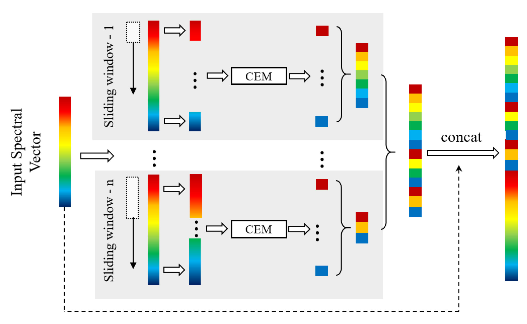
2.3. Ensemble based Cascaded CEM Detector

E-CEM detector consists of two stages, (1) “multi-scale scanning” stage and (2) “cascaded detection” stage. In the first stage, the input is a spectral vector while the output is a feature vector containing multi-scale spectral information, which aims to extract the features of the spectrum and to enhance the robustness to spectrum changes. In the second stage, the input is the feature vector produced by the multi-scale scanning stage, while the output is the final detection score, where the higher the score, the more likely the current spectrum is a target. In this stage, we use a cascaded detection structure with sigmoid nonlinear transformation to enhance the nonlinear discrimination ability of the detector. Besides, we also use multiple CEM detectors in each layer to further improve the robustness to spectral changes. Figure 1 shows an illustration of the E-CEM detector.

2.3.1. Multi-Scale Scanning

The multi-scale scanning stage consists of several parallel units. Similar to the processing pipeline of the deep forest algorithm [45], in each unit, we use a sliding window with a particular size to scan and crop the spectrum into a set of spectral fragments, and then each spectral fragment is processed and concatenated as the output of this unit. Then, the outputs of all the units and the original spectral vector are concatenated together to finally produce the output feature vector of this stage. Figure 2 shows the process of multi-scale scanning.

Specifically, suppose that the size of the sliding window of the current unit is l, the stride of the window is s and the input of this unit is a spectral vector $\mathbf{r}=[r_1,r_2,\dots ,r_D]\in {\mathbb{R}}^{D\times 1}$. The entire multi-scale scanning process can be expressed as the following steps. First, slide the window on the spectrum with the length l and the stride s and crop it into K fragments:

$$\begin{array}{c}{\widehat{\mathbf{r}}}_1={[r_1,r_2,\dots ,r_l]}^T\hfill \\ {\widehat{\mathbf{r}}}_2={[r_{1+s},r_{2+s},\dots ,r_{l+s}]}^T\hfill \\ \cdots \hfill \end{array}$$

(5)

For N pixels, we have $NK$ fragments in total. The pixel here refers to the spectral vector, which is a vector with spectral dimension of D and spatial dimension of 1. For simplicity, we refer to it as a “pixel”. Then, we use a CEM detector to process each of the fragments. For each window location, a CEM detector is constructed by using the fragments of all pixels of this location and gives the corresponding outputs: ${\nu }_i,i=1,\dots ,k$. By concatenating them together, the feature vector of the current unit will have the following expression: ${\mathbf{\nu }}_l={[{\nu }_1,{\nu }_2,\dots ,{\nu }_k]}^T\in {\mathbb{R}}^{k\times 1}$. Finally, by concatenating the output of each unit and the original spectral vector $\mathbf{r}$, the output feature vector of the multi-scale scanning stage can be represented as:

$$\tilde{\mathbf{r}}=[{\mathbf{\nu }}_{l_1};{\mathbf{\nu }}_{l_2},\dots ;{\mathbf{\nu }}_{l_n};\mathbf{r}]\in {\mathbb{R}}^{(nK+D)\times 1},$$

(6)

where $l_1,\dots ,l_n$ represents the window size of each unit and n represents the total number of scanning units.

2.3.2. Cascaded Detection

Cascaded detection consists of multiple detection layers. The input of this stage is the spectrum feature vector produced by the multi-scale scanning stage, while the output is E-CEM’s detection score. The output score of each detection layer is used for transforming the feature vector and then serves as the input of the next layer. Then, a new detection score can be obtained based on the transformed feature. In addition, in each layer, we design m different CEM detectors with random regularization coefficients ${\lambda }_1,\dots ,{\lambda }_m$ to enhance the detector’s generalization ability. In our model, instead of using fixed $\lambda$, we set it as a random variable. In the ensemble learning, there are two groups of classic algorithms, one group is boosting, and another group is bagging. For bagging algorithms, increasing the diversity of each base model will effectively improve the stability of final prediction [46]. The random forest [46], which is a representative of bagging method, increases the difference of each model by randomly sampling features. Similarly, in our method, we have the similar purpose set different $\lambda$ in different base detectors, that is, to further increase the divergence of the each model to improve the final detection’s robustness. As for how $\lambda$ affects the detection result, we investigate two extreme cases, one is that $\lambda$ is equal to 0, and the other is that $\lambda$ is infinite. When $\lambda$ is set to 0, the regularized CEM will become the original CEM:

$$\underset{\lambda \to +0}{\lim }\mathbf{\omega }\left(\lambda \right)=\underset{\lambda \to +0}{\lim }\frac{{(\mathbf{R}+\lambda \mathbf{I})}^{-1}\omega }{{\mathbf{d}}^T{(\mathbf{R}+\lambda \mathbf{I})}^{-1}\mathbf{d}}=\frac{{\mathbf{R}}^{-1}\mathbf{d}}{{\mathbf{d}}^T{\mathbf{R}}^{-1}\mathbf{d}}.$$

(7)

When $\lambda$ is set to infinite, $\omega$ will become independent of $\mathbf{R}$ and will have the same direction as that of the target spectrum $\mathbf{d}$. This is because:

$$\underset{\lambda \to +\infty }{\lim }\mathbf{\omega }\left(\lambda \right)=\underset{\lambda \to +\infty }{\lim }\frac{{(\mathbf{R}+\lambda \mathbf{I})}^{-1}\omega }{{\mathbf{d}}^T{(\mathbf{R}+\lambda \mathbf{I})}^{-1}\mathbf{d}}=\frac{\mathbf{d}}{{\mathbf{d}}^T\mathbf{d}}.$$

(8)

Therefore, in the case of $\lambda$ is infinite, the detection will be the projection of the spectral vector in the d direction, which can be considered as the simplest “spectral matching” method. The above discussion indicates that $\lambda$ can be considered as the tradeoff between the original CEM and the projection in the $\mathbf{d}$ direction.

Suppose the input feature vector of layer t is ${\tilde{\mathbf{r}}}_t$, and the output scores of m CEM detectors are $u_1,u_2,\dots ,u_m$, then the average score of these detectors can be written as:

$$\begin{array}{cc}\hfill \overline{u}& =\frac{1}{m}\sum _{i=1}^m\mathbf{\omega }{\left({\lambda }_i\right)}^T{\tilde{\mathbf{r}}}_t\hfill \\ & =\frac{1}{m}\sum _{i=1}^m\frac{{\mathbf{d}}^T{(\mathbf{R}+{\lambda }_i\mathbf{I})}^{-1}{\tilde{\mathbf{r}}}_t}{{\mathbf{d}}^T{(\mathbf{R}+{\lambda }_i\mathbf{I})}^{-1}\mathbf{d}},\hfill \end{array}$$

(9)

where $\mathbf{\omega }\left({\lambda }_i\right)$ is the coefficients of the ith CEM detector. Then, the feature vector ${\tilde{\mathbf{r}}}_t$ of the current layer is transformed into a new feature vector as the input of the next layer according to $\overline{u}$:

$${\tilde{\mathbf{r}}}_{t+1}={\tilde{\mathbf{r}}}_{t}h\left(\overline{u}\right)$$

(10)

We use the sigmoid function, which is commonly used in neural networks [29], as our nonlinear transformation function. This function has the following expression:

$$h\left(x\right)=1/(1+e^{-x}).$$

(11)

This function indicates that the features with small outputs will be suppressed while those with large outputs will be unchanged. After several layers, the average score of the last layer $\overline{u}$ is used as the detection output of the E-CEM algorithm.

Since our method is inspired by the cascaded structure in deep learning, it does have some similarities with CNN in terms of the processing pipeline. For example, CEM can be regarded as the convolution unit and the output can be regarded as the feature map. However, the difference between our method and CNN is that the output of the CEMs $h\left(\overline{u}\right)$ is just a probability and does not contain the spectral information, in order to better transfer the spectral information to subsequent layers, the spectral vector is multiplied with the output.

In addition, there is another advantage of using multiplication, i.e., it can be considered as an integration of attention mechanism. Since higher scores pixels are more likely to be the target, while the lower scores pixels are more likely to be the background, so, after multiplying, target pixels are retained, and background pixels are suppressed. In this way, in the subsequent layers, the target pixels will receive more attention to get better detection results.

3. Experiments, Results and Discussion

To evaluate the effectiveness of the proposed E-CEM algorithm, we compare it with eight popular hyperspectral target detection algorithms, including CEM [2], ACE [10], MF [11], SID [9], TVD [15], RHMF [16], RACE [37], and HCEM [17] on one synthetic hyperspectral image and two real hyperspectral images. Among these algorithms, the former four are classical detection algorithms. TVD and RHMF are two recent improvements of CEM detector by considering the local similarity constraint and high order statistics. RACE and HCEM are cascaded detectors and are the most similar ones with our method. In these two detectors, the traditional ACE/CEM detector is used as a basic detector in each layer, and the target/background spectra are iteratively updated based on the previous layer’s detection outputs. In the HCEM detector, in each layer of detection, the CEM’s output of each spectrum is transformed by a nonlinear suppression function and then considered as a coefficient multiplied on this spectrum for the next round of iteration. The authors theoretically proved the convergency of the HCEM and gave a theoretically explanation that why they can obtain the gradually increasing detection performance. In the RACE detector, an ACE detector is used as a basic detector in each layer, and the target spectrum is revised iteratively based on the last layer’s detection outputs to generate the “optimal” target spectrum. Finally, the authors use the “optimal” target spectrum to obtain the final detection result.

The codes of TVD, RHMF, RACE, and HCEM are provided by their authors, while the other four classical algorithms are implemented by ourselves. The code of our algorithm will be made publicly available at levir.buaa.edu.cn/Code.htm.

3.1. Data Used

The experiments are conducted on one synthetic image data, and two real hyperspectral image data: AVIRIS San Diego Data and AVIRIS Cuprite Data.

3.1.1. Synthetic Data

The synthetic hyperspectral image we used is generated from the United States Geological Survey (USGS) digital spectral library [47]. 15 endmember spectra are used for data synthesis, including Axinite HS342.3B, Rhodochrosite HS67, Chrysocolla HS297.3B, Niter GDS43 (K-Saltpeter), Anthophyllite HS286.3B, Neodymium Oxide GDS34, Monazite HS255.3B, Samarium Oxide GDS36, Pigeonite HS199.3B, Meionite WS700.HLsep, Spodumene HS210.3B, Labradorite HS17.3B, Grossular WS484, Zoisite HS347.3B, and Wollastonite HS348.3B. The reflectance values of these 15 kinds of materials are collected in 224 bands, and the wavelength lies in 0.4∼2.5 $\mathsf{\mu }$m.

The Labradorite HS17.3B is used as the target of interest. We use the data generation and target implantation method introduced by Chang et al. [48] to generate the synthetic data. Specifically, we first divide the synthetic map, whose size is $s^2\times s^2$ ($s=8$), into $s\times s$ regions, where each region is initialized with the same type of ground cover that randomly selected from the above 15 kinds of spectra. We implant clean target into the backgrounds by replacing their corresponding pixels. To evaluate the detector’s performance on mixed spectral data, we first mix the synthetic map through a $(s+1)\times (s+1)$ spatial low-pass filter so that there is no pure pixel in the synthetic image. To evaluate the algorithm’s robustness to spectral variation, all pixels including both targets and backgrounds are corrupted by a Gaussian white noise Signal-to-Noise Ratio (SNR) of 20 dB and 25 dB. Figure 3a shows the first band of the synthetic image. Figure 3b shows its ground truth. The synthetic image size is $64\times 64$ and the total number of target pixels is 12. SNR is defined as follows:

$$SNR\left(dB\right)=10{\log }_{10}\frac{P_{signal}}{P_{noise}},$$

(12)

where $P_{signal}$ represents the power of signal and $P_{noise}$ represents the power of noise.

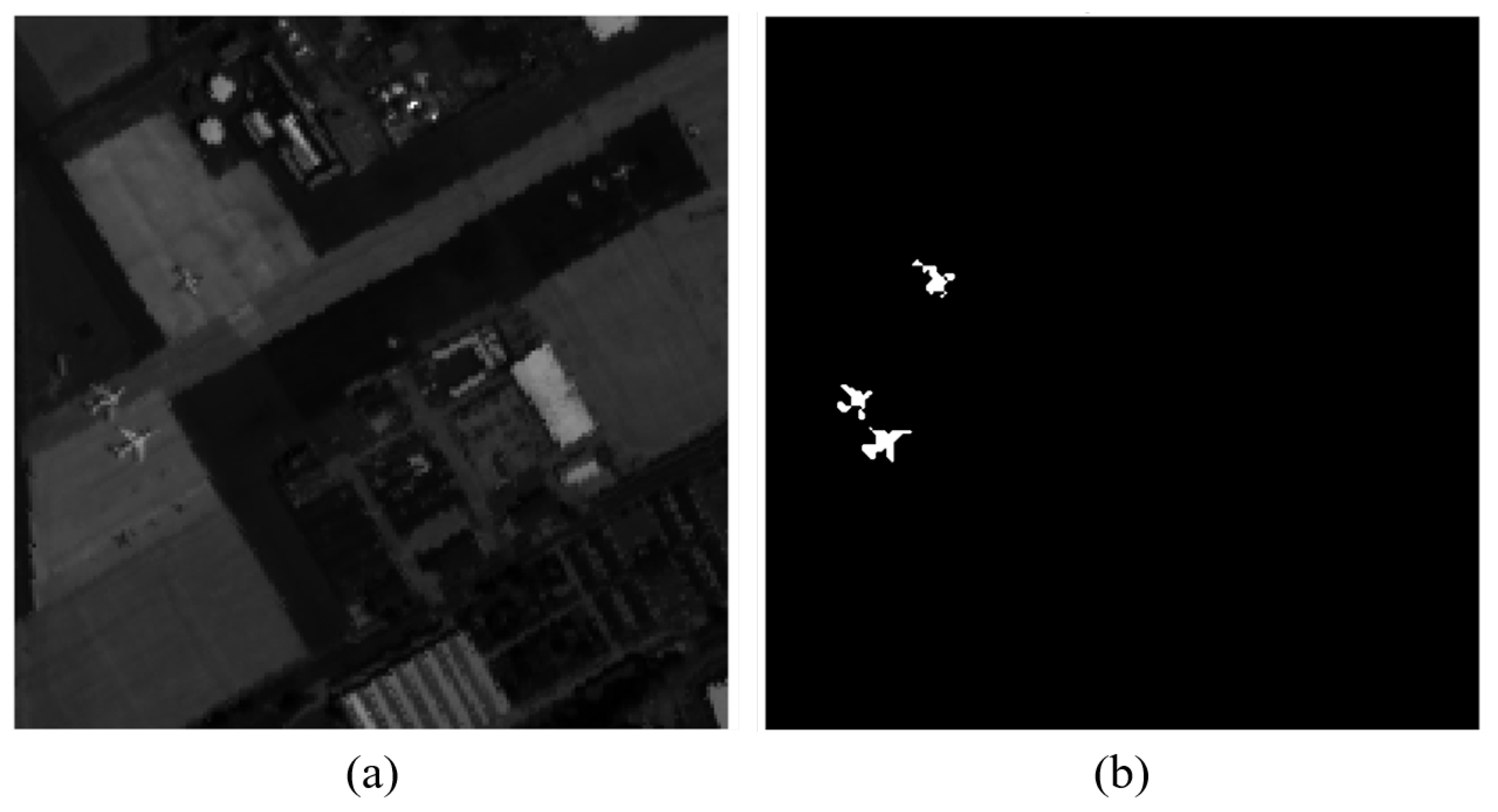
3.1.2. AVIRIS San Diego Data

Two real hyperspectral images collected by the Spectrometer Visible/Infrared Imaging Spectrometer (AVIRIS) are used for evaluating the algorithms. AVIRIS is the first full spectral range imaging spectrometer and dedicated to earth remote measurement [49]. The spectrometer delivers calibrated images of the upwelling spectral radiance in 224 contiguous spectral channels (bands) with wavelengths from 0.38 to 2.51 $\mathsf{\mu }$m.

The AVIRIS San Diego Data we used was captured at San Diego, America. It contains a part of an airport. The targets are three airplanes and the backgrounds are farmland, buildings, and runways. The total number of target pixels is 134. The target spectrum $\mathbf{d}$ is obtained by averaging all spectra within the target regions. The size of each band is in 200 × 200 pixels. After removing the low SNR and water vapor absorption bands, a total of 189 bands are used to conduct the experiments. Figure 4a shows the first band of the hyperspectral image. Figure 4b shows its ground truth. All the above-mentioned algorithms and the proposed E-CEM algorithm are tested on this data.

3.1.3. AVIRIS Cuprite Data

The AVIRIS Cuprite Data [50] is used to test our algorithm. This image was captured by AVIRIS in the Cuprite mining district of Nevada in 1997. There are about 14 kinds of mineral in this image, including buddingtonite, Na-Montmorillonite, Nontronite (Fe clay), Kaolinite-wxl, etc. Figure 5a shows the minerals map [51] which is produced by the Tricorder 3.3 software. We use a 250 × 191 pixel subset of this image to conduct our experiment, which is marked by the red box in this figure. The buddingtonite is selected as the target, which occupies 39 pixels. Figure 5b shows the first band of the image and Figure 5c shows the distribution of the buddingtonite targets. After removing the low SNR and water absorption bands, 188 bands are left to conduct our experiment. As there are two spectra for buddingtonite in the USGS Digital Spectral Library [47], we use their average as the target spectrum for all algorithms. The reason why we choose “buddingtonite” for detection is that this mineral is difficult to detect and the number of pixels of this material is moderate. More importantly, many previous target detection papers [15,16,17] have used buddingtonite as the target. In order to make a fairer comparison with previous methods, we use it as the target.

3.2. Experimental Setup and Evaluation Metrics

In all of our experiments, we use the same parameter configuration for E-CEM detector:

• In the multi-scale scanning stage, we set the number of windows to $n=4$ and the window size to $l_i=\frac{i}{4}D,i=1,\dots ,4$, where D is the number of bands.
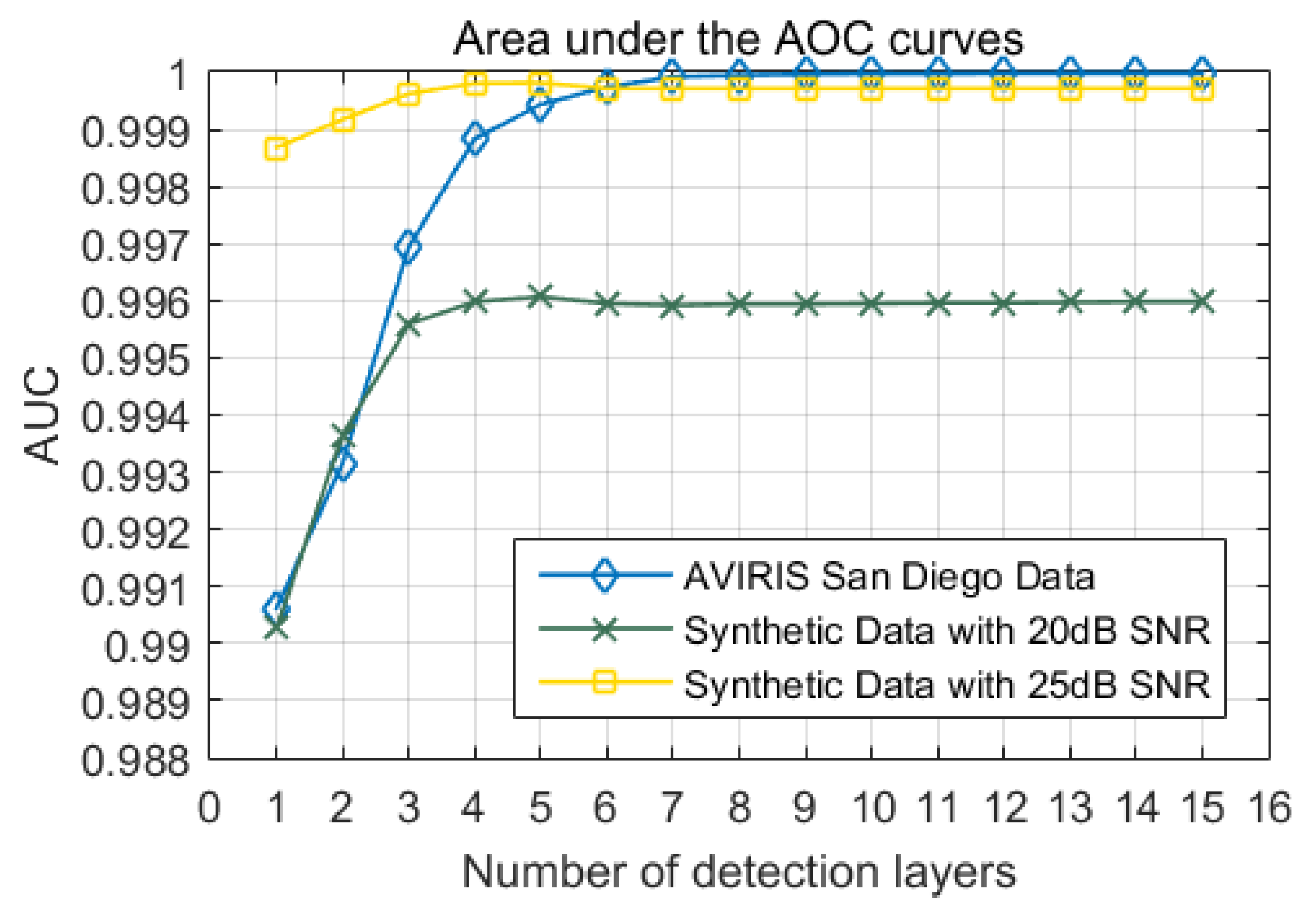
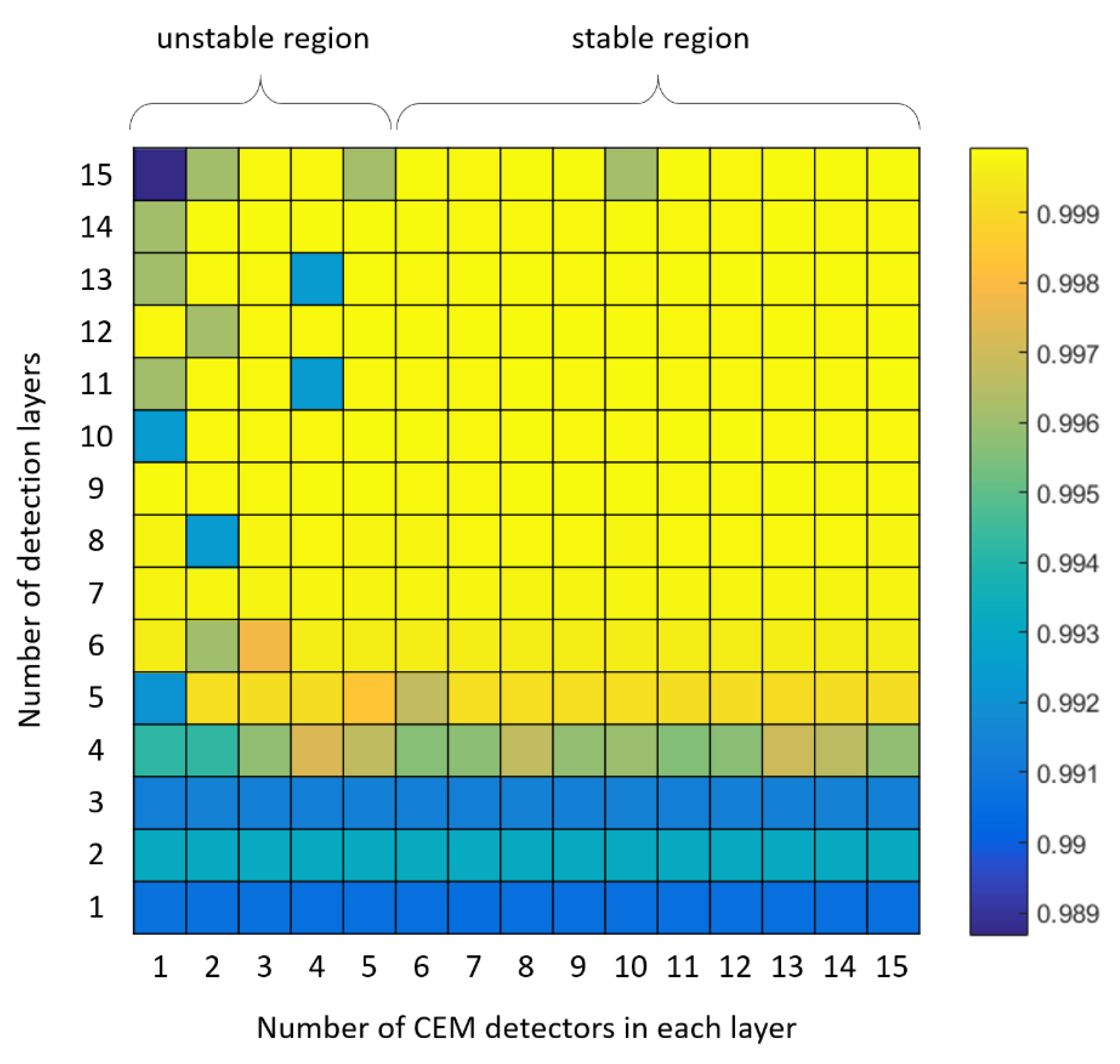
• In the cascaded detection stage, we set the number of detection layers to $k=10$ and the number of CEMs per layer to $m=6$.

To evaluate the algorithm quantitatively, we use the Receiver Operating Characteristic (ROC) curve [17] to evaluate the detection results. The ROC curve describes the relationship between False alarm rate ($Fa$) and Probability of detection ($Pd$). $Fa$ and $Pd$ are defined as follows:

$$Fa=\frac{N_f}{N},Pd=\frac{N_c}{N_t},$$

(13)

where $N_f$ represents the number of pixels of false alarms in the image; $N_c$ represents the number of correctly detected target pixels; $N_t$ represents the number of target pixels; N represents the number of all pixels in the image. Clearly, under the same $Fa$, the higher the $Pd$, the better detection performance is.

3.3. Detection Results on Synthetic Data

The detection outputs of all detectors on synthetic data (with 20dB SNR Gaussian white noise) are shown in Figure 6. The first row of this figure shows the E-CEM detection output scores of its 1st, 2nd, 3rd, 5th and 10th layer. The second and third rows show the detection output of other comparison algorithms. As we can see, when the number of detection layers increases, the output scores of the target pixels are gradually enhanced while that of the background pixels are suppressed. All output scores are normalized to $[0,1]$ for a fair comparison. Figure 7 shows their ROC curves. Both of the ROC curves and the detection outputs suggest that E-CEM achieves better detection results than other algorithms and it is more robust to noise interference. As there are no pure pixels in the synthetic image, experimental results demonstrate that the E-CEM is also robust to spectrum changes caused by mixed pixels.

As the ROC curves tend to “saturate” at a high recall rate, to make a more comprehensive evaluation of these algorithms, we further use the Area Under the Curve (AUC) of ROC as another quantitative evaluation criterion. In order to avoid the randomness of the results, for synthetic data experiment, we have repeated 10 times to randomly generate each group of synthetic data by randomly adding noise.

Table 1. The mean and standard deviation of the area under the ROC curve of different algorithms on synthetic data under the interference of white Gaussian noise.

Method	Noise of 20 dB SNR		Noise of 25 dB SNR
	Mean	Standard Deviation	Mean	Standard Deviation
CEM [2]	0.97957	5.29$\times {10}^{-3}$	0.99733	1.13$\times {10}^{-3}$
ACE [10]	0.96998	4.47$\times {10}^{-3}$	0.99653	2.19$\times {10}^{-3}$
MF [11]	0.97549	4.04$\times {10}^{-3}$	0.9892	1.33$\times {10}^{-3}$
SID [9]	0.55201	3.86$\times {10}^{-3}$	0.88742	1.70$\times {10}^{-3}$
HCEM [17]	0.99221	6.81$\times {10}^{-3}$	0.99801	5.24$\times {10}^{-3}$
TVD [15]	0.96270	8.63$\times {10}^{-3}$	0.97745	3.62$\times {10}^{-3}$
RACE [37]	0.98732	2.14$\times {10}^{-3}$	0.99335	9.47$\times {10}^{-4}$
RHMF [16]	0.98884	8.32$\times {10}^{-3}$	0.99773	1.68$\times {10}^{-3}$
E-CEM (ours)	0.99941	2.47$\times {10}^{-4}$	0.99995	3.13$\times {10}^{-5}$

shows the mean and standard deviation of AUC values of the nine algorithms on the synthetic data under the interference of white Gaussian noise with different SNR. Experimental results show that E-CEM has a higher average score and a lower standard deviation than other algorithms. This indicates that E-CEM is more robust than other algorithms while achieving higher detection accuracy.

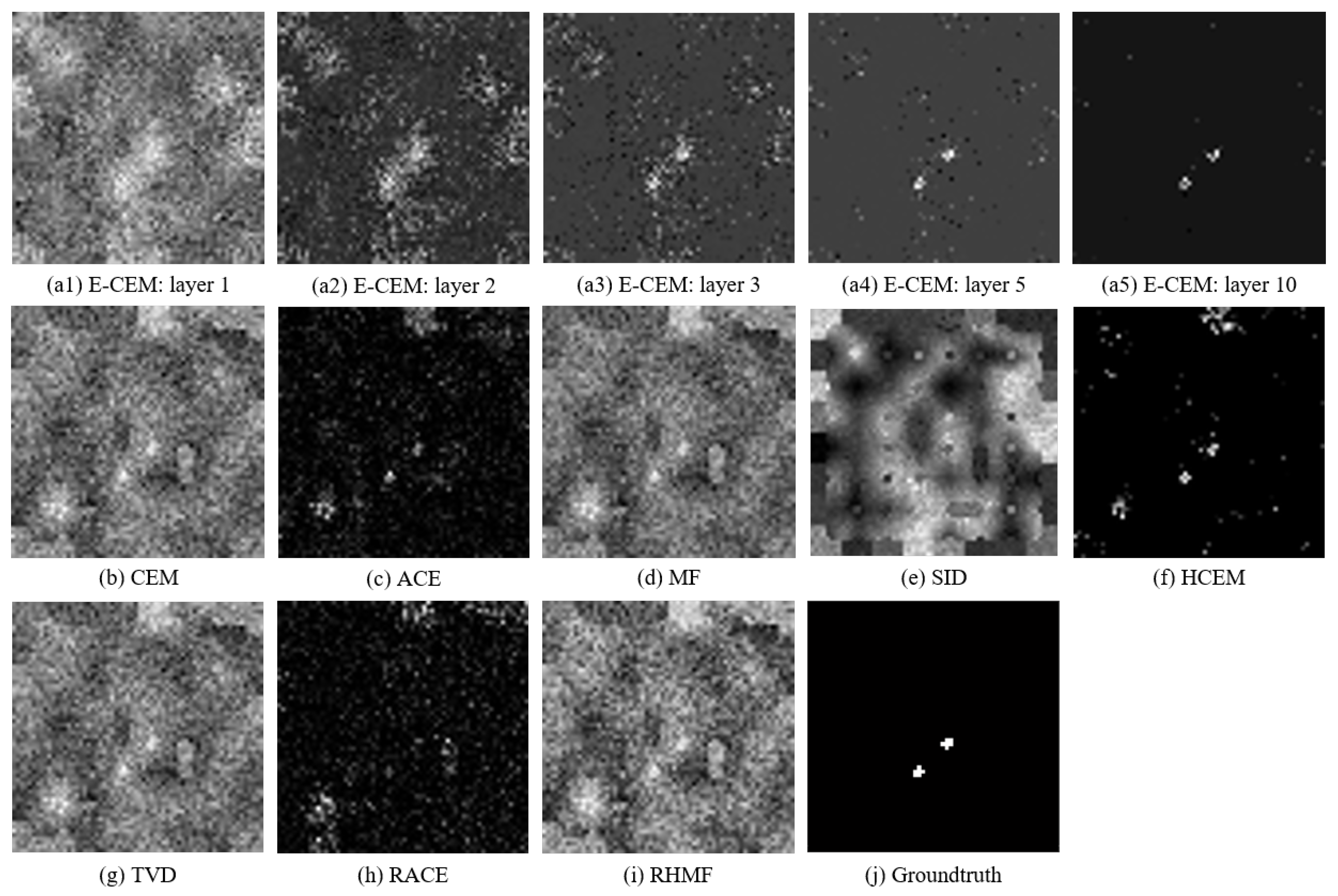
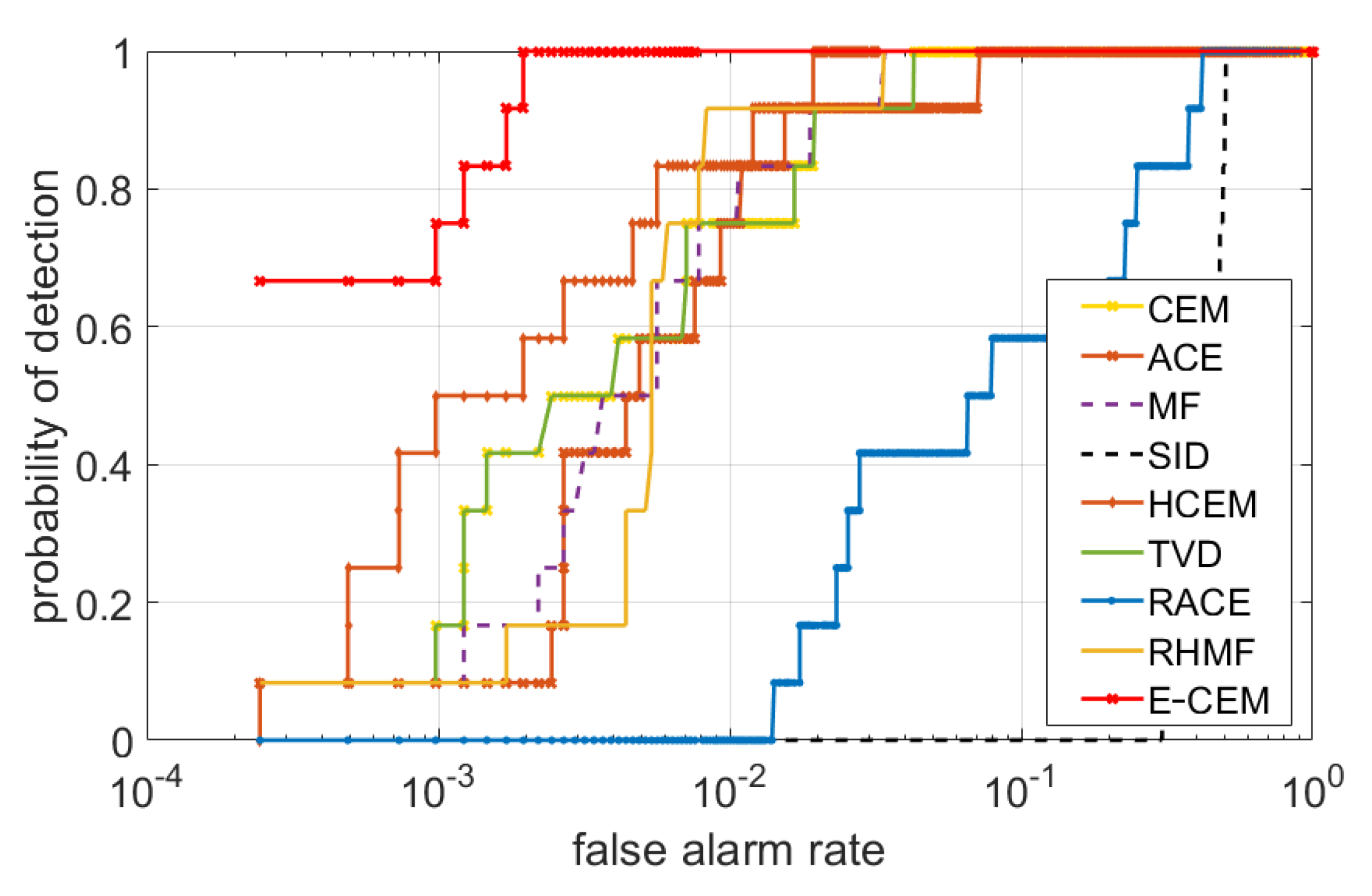
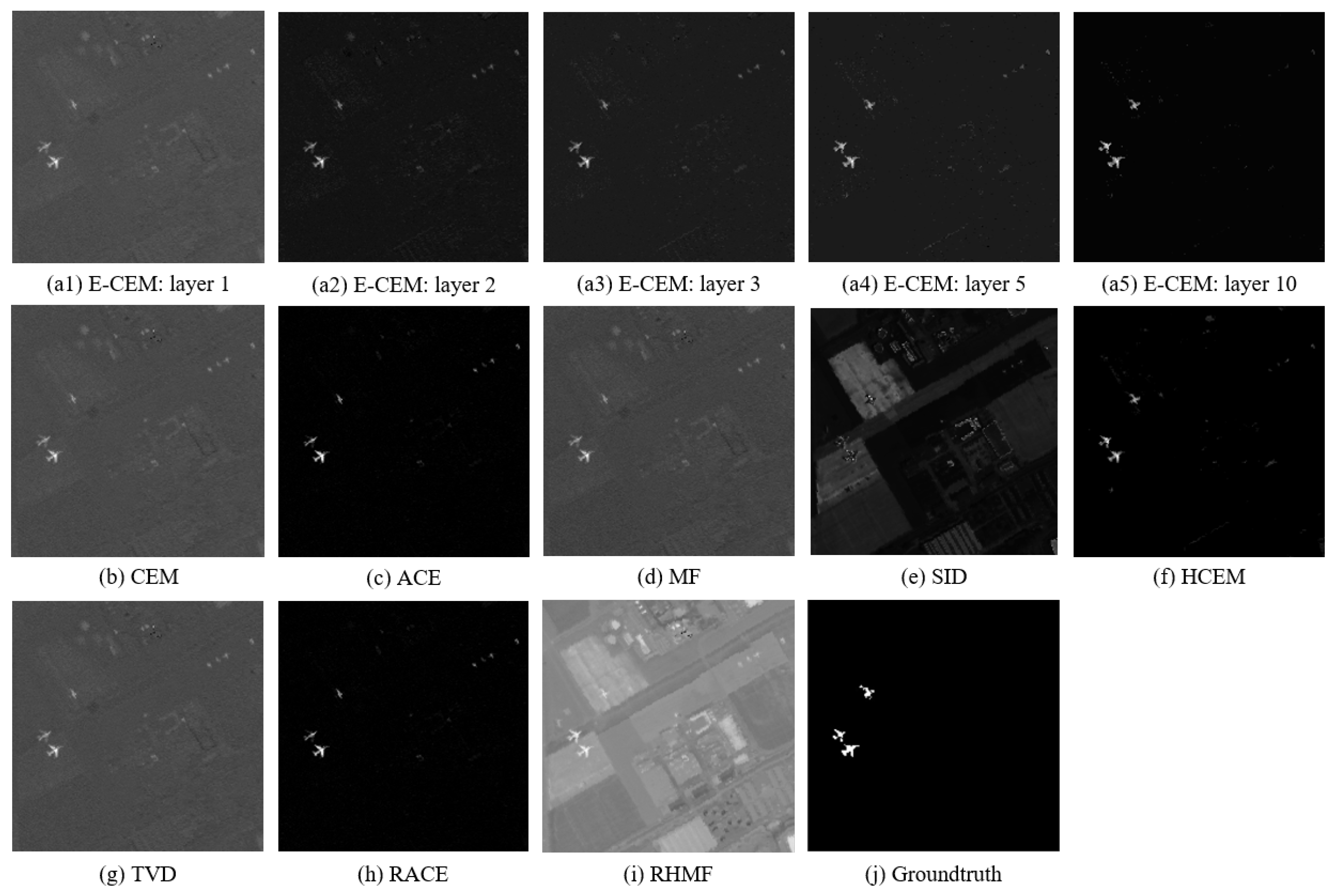
3.4. Detection Results on AVIRIS San Diego Data

Figure 8 shows the detection score maps of the different algorithm on AVIRIS San Diego data. The first row of this figure shows the E-CEM detection score maps of its 1st, 2nd, 3rd, 5th and 10th layer. The second and third rows show the detection output of other comparison algorithms. We can again observe the increasing performance of the detector with the increasing number of stacking layers. All output values are scaled to $[0,1]$ for a fair comparison. Figure 9 shows their ROC curves. Our algorithm is among the best entries of the detection results.

Similar to the synthetic data generation process, we also add additional Gaussian white noise to the AVIRIS San Diego data to increase the detection difficulty.

Table 2. The area under the ROC curve of different algorithms on AVIRIS San Diego data under the interference of white Gaussian noise with different SNR.

Method	San Diego Data
	w/o Noise	20 dB SNR	25 dB SNR
CEM [2]	0.99047	0.98398	0.98573
ACE [10]	0.97882	0.97841	0.97894
MF [11]	0.99078	0.98396	0.98584
SID [9]	0.81225	0.81659	0.81507
HCEM [17]	0.99571	0.97173	0.97977
TVD [15]	0.99046	0.98398	0.98573
RACE [37]	0.97882	0.97842	0.97894
RHMF [16]	0.98982	0.98284	0.98543
E-CEM (ours)	0.99988	0.98540	0.99356

shows the AUC values of the nine algorithms on AVIRIS San Diego data under the interference of white Gaussian noise with different SNR. We observe the better performance of our method over other detection algorithms.

3.5. Detection Results on AVIRIS Cuprite Data

Figure 10 shows the detection output scores of different algorithms on AVIRIS Cuprite data, where (a1)–(a5) are the 1st, 2nd, 3rd, 5th, and 10th layers’ output of the proposed E-CEM algorithm, (b)–(i) are the other eight detection algorithms, (j) is the ground truth. All outputs are scaled to $[0,1]$ for a fair comparison. Since the publicly available Cuprite data were obtained by AVIRIS in 1997 while the corresponding ground truth was produced by Tricorder software in 1995 [52], we can only make a qualitative analysis of the different detection outputs on this data. Therefore, we do not plot their ROC curves. We notice that RACE fails to detect the target. This is because the amount of target pixels in this image is too small and the vast number of the undesired background will overwhelm the updating process of the “target” spectrum.

3.6. Parameters Analysis

We also design three ablation experiments to analyze the importance of each technical component of our method, including the “cascaded detection”, “random averaging” and “multi-scale scanning”. All the ablation experiments are quantitatively performed on the AVIRIS San Diego data and the synthetic data.

• How important is cascaded detection

As we introduced in Section 2.3, the detection of the proposed E-CEM is processed in a cascaded detection paradigm. Therefore, the number of detection layer is an important configuration of our method. The effect of the cascaded detection can be analyzed by setting the number of layers to $k=1\sim 15$, without changing other parameter configurations. Figure 11 shows the AUC values of each layer’s detection outputs on AVIRIS San Diego data and synthetic data. Compared with non-cascaded detection (number of layers $k=1$), we can observe significant improvement of the detection results by using the cascaded detection strategy. In addition to that, the detection performance also increases with the increase in the number of layers. As the results begin to saturate after stacking 10 layers, to balance the accuracy and time efficiency, the default setting of the layer number is $k=10$.

• How important is multi-scale scanning

To evaluate the effectiveness of the “multi-scale scanning” strategy, we designed 5 scanning modes with a different number of windows and different window size.

Table 3. AUC of E-CEM with a different number of sliding windows n on San Diego Data. D is the number of bands.

n	Window Wize	AUC
1	$\left[D\right]$ (no sliding window)	0.9916
2	$[1/2,1]D$	0.9923
4	$[1/4,2/4,3/4,1]D$	0.9999
6	$[1/6,2/6,3/6,4/6,5/6,1]D$	0.9999
8	$[1/8,2/8,3/8,4/8,5/8,6/8,7/8,1]D$	0.9999

shows their AUC values on San Diego data. There is a noticeable improvement in the detection results when applying “multi-scale scanning”. When the number of scanning windows is larger than 4, there is very little improvement. To balance the accuracy and time efficiency, we choose $[\frac{1}{4}D,\frac{2}{4}D,\frac{3}{4}D,D]$ as the default setting of the scanning windows.

• How important is random averaging

The ensemble is an important strategy in our methods to improve its robustness and generalization ability. To evaluate the effectiveness of the random averaging of multiple CEM detectors in each detection layer, we set the number of detectors in each layer to $m=1\sim 15$ and compare their detection results. Figure 12 shows the AUC values with different combinations of layer numbers and detector numbers in each layer on San Diego data. We can see when the $m\le 5$, the performance of E-CEM detectors will be unstable as the number of layers increases. When $m>5$, E-CEM will have more stable results. To balance the robustness and time efficiency, we choose $m=6$ as our default setting.

• Analysis on the regularization parameter $\lambda$

In order to compare the performance of our method on using a constant regularization coefficient and random regularization coefficient, we have made the an experiment on the synthetic data with different settings of regularization coefficient and

Table 4. The area under the ROC curve of E-CEM with different regularization coefficient $\lambda$ on synthetic data under the interference of white Gaussian noise.

t	Noise of 20 dB SNR		Noise of 25 dB SNR
	$\mathbf{\lambda }$ = constant(t)	$\mathbf{\lambda }$ = random (0,t)	$\mathbf{\lambda }$ = constant (t)	$\mathbf{\lambda }$ = random(0,t)
0.01	0.91310	0.99800	0.99990	0.99997
0.02	0.99520	0.99886	0.99982	0.99994
0.05	0.99669	0.99941	0.99857	0.99995
0.08	0.99051	0.99949	0.99494	0.99996
0.10	0.98198	0.99794	0.98939	0.99980

shows the area under the ROC curve of our method. The experimental result suggests that the E-CEM achieves more stable and better performance when random $\lambda$ is used. The experimental result also suggests that when there is stronger noise (SNR reduced from 25 dB to 20 dB), the model needs a larger $\lambda$ to achieve better performance.

3.7. Speed Performance

To compare the speed performance of the algorithms, we test them on the same computer with a 4.00 GHz Intel Core i7 CPU and 32 GB of memory. The computational time of E-CEM and other algorithms on the synthetic data, AVIRIS San diego Data and AVIRIS Cuprite data is listed in

Table 5. The computational time (second) of different algorithms on synthetic data, AVIRIS San diego Data and AVIRIS Cuprite data.

Method	Synthetic Data	San Diego Data	Cuprite Data
CEM [2]	0.04	0.11	0.08
ACE [10]	0.04	0.17	0.20
MF [11]	0.02	0.08	0.07
SID [9]	0.07	0.53	0.94
HCEM [17]	5.18	5.89	7.08
TVD [15]	2.07	6.38	2.21
RACE [37]	0.51	1.16	1.24
RHMF [16]	4.82	43.77	21.08
E-CEM (ours)	2.58	13.02	15.35

.

Although the proposed E-CEM is slower than classical algorithms such as CEM and ACE, when comparing with some recent algorithms, it has comparable speed performance. For example, on San Diego data and Cuprite data, our algorithm is faster than RHMF. On Synthetic data, our algorithm is faster than RHMF and HCEM.

4. Conclusions

The nonlinear discrimination ability and generalization ability are two important factors for machine learning algorithms. Inspired by the ensemble learning method, we propose a new hyperspectral image target detection algorithm named Ensemble based Constrained Energy Minimization (E-CEM) that takes into account both of the above factors. E-CEM is designed with the help of the ensemble method by integrating a number of techniques including “cascaded detection”, “random averaging” and “multi-scale scanning” so that to improve both of its nonlinear discrimination ability and generalization ability. Experimental results on one synthetic data and two real hyperspectral data demonstrate the effectiveness of these techniques. Compared with the classical hyperspectral target detection algorithms and their recent improved versions, E-CEM has higher detection accuracy and is more robust to the interference of noise and spectrum changes. Since the proposed ensemble based cascaded framework is scalable, flexible and shows promising results under extensive experimental verification, in our future work, we will focus on improving other classical algorithms such as MF, ACE, etc, by using ensemble techniques and improving their detection speed.

References

1. DiPietro, R.S.; Truslow, E.; Manolakis, D.G.; Golowich, S.E.; Lockwood, R.B. False-alarm characterization in hyperspectral gas-detection applications. Imaging Spectrom. XVII 2012, 8515, 85150I. [Google Scholar]
2. Farrand, W.H.; Harsanyi, J.C. Mapping the distribution of mine tailings in the Coeur d’Alene River Valley, Idaho, through the use of a constrained energy minimization technique. Remote Sens. Environ. 1997, 59, 64–76. [Google Scholar] [CrossRef]
3. Tiwari, K.; Arora, M.; Singh, D. An assessment of independent component analysis for detection of military targets from hyperspectral images. Int. J. Appl. Earth Obs. Geoinf. 2011, 13, 730–740. [Google Scholar] [CrossRef]
4. Winter, E.M.; Miller, M.A.; Simi, C.G.; Hill, A.B.; Williams, T.J.; Hampton, D.; Wood, M.; Zadnick, J.; Sviland, M.D. Mine detection experiments using hyperspectral sensors. In Proceedings of the Defense and Security, 2004, Orlando, FL, USA, 21 Sptember 2004; Volume 5415, pp. 1035–1042. [Google Scholar]
5. Lin, C.; Chen, S.Y.; Chen, C.C.; Tai, C.H. Detecting newly grown tree leaves from unmanned-aerial-vehicle images using hyperspectral target detection techniques. ISPRS J. Photogramm. Remote Sens. 2018, 142, 174–189. [Google Scholar] [CrossRef]
6. Rahimzadegan, M.; Sadeghi, B.; Masoumi, M.; Ghalehjoghi, S.T. Application of target detection algorithms to identification of iron oxides using ASTER images: A case study in the North of Semnan province, Iran. Arab. J. Geosci. 2015, 8, 7321–7331. [Google Scholar] [CrossRef]
7. Eismann, M.T.; Stocker, A.D.; Nasrabadi, N.M. Automated hyperspectral cueing for civilian search and rescue. Proc. IEEE 2009, 97, 1031–1055. [Google Scholar] [CrossRef]
8. Kruse, F.A.; Lefkoff, A.; Boardman, J.; Heidebrecht, K.; Shapiro, A.; Barloon, P.; Goetz, A. The spectral image processing system (SIPS)—interactive visualization and analysis of imaging spectrometer data. Remote Sens. Environ. 1993, 44, 145–163. [Google Scholar] [CrossRef]
9. Chang, C.I. An information-theoretic approach to spectral variability, similarity, and discrimination for hyperspectral image analysis. IEEE Trans. Inf. Theory 2000, 46, 1927–1932. [Google Scholar] [CrossRef] [Green Version]
10. Manolakis, D.; Marden, D.; Shaw, G.A. Hyperspectral image processing for automatic target detection applications. Lincoln Lab. J. 2003, 14, 79–116. [Google Scholar]
11. Manolakis, D.; Lockwood, R.; Cooley, T.; Jacobson, J. Is there a best hyperspectral detection algorithm? SPIE 2009, 7334, 733402. [Google Scholar]
12. Scharf, L.L.; Friedlander, B. Matched subspace detectors. IEEE Trans. Signal Process. 1994, 42, 2146–2157. [Google Scholar] [CrossRef]
13. Wang, Z.; Xue, J.H. Matched shrunken subspace detectors for hyperspectral target detection. Neurocomputing 2018, 272, 226–236. [Google Scholar] [CrossRef] [Green Version]
14. Yang, S.; Shi, Z.; Tang, W. Robust hyperspectral image target detection using an inequality constraint. IEEE Trans. Geosci. Remote Sens. 2015, 53, 3389–3404. [Google Scholar] [CrossRef]
15. Yang, S.; Shi, Z. Hyperspectral image target detection improvement based on total variation. IEEE Trans. Image Process. 2016, 25, 2249–2258. [Google Scholar] [CrossRef] [PubMed]
16. Shi, Z.; Yang, S. Robust high-order matched filter for hyperspectral target detection. Electron. Lett. 2010, 46, 1065–1066. [Google Scholar] [CrossRef]
17. Zou, Z.; Shi, Z. Hierarchical suppression method for hyperspectral target detection. IEEE Trans. Geosci. Remote Sens. 2016, 54, 330–342. [Google Scholar] [CrossRef]
18. Harsanyi, J.C.; Chang, C.I. Hyperspectral image classification and dimensionality reduction: An orthogonal subspace projection approach. IEEE Trans. Geosci. Remote Sens. 1994, 32, 779–785. [Google Scholar] [CrossRef]
19. Bernabe, S.; Sanchez, S.; Plaza, A.; López, S.; Benediktsson, J.A.; Sarmiento, R. Hyperspectral unmixing on GPUs and multi-core processors: A comparison. IEEE J. Sel. Topics Appl. Earth Obs. Remote Sens. 2013, 6, 1386–1398. [Google Scholar] [CrossRef]
20. Kay, S.M. Fundamentals of Statistical Signal Processing; Prentice Hall PTR: Upper Saddle River, NJ, USA, 1993. [Google Scholar]
21. Manolakis, D.G. Realistic matched filter performance prediction for hyperspectral target detection. Opt. Eng. 2005, 44, 116401. [Google Scholar] [CrossRef]
22. Schweizer, S.M.; Moura, J.M. Efficient detection in hyperspectral imagery. IEEE Trans. Image Process. 2001, 10, 584–597. [Google Scholar] [CrossRef]
23. Schweizer, S.M.; Moura, J.M. Hyperspectral imagery: Clutter adaptation in anomaly detection. IEEE Trans. Inf. Theory 2000, 46, 1855–1871. [Google Scholar] [CrossRef]
24. Chen, Y.; Nasrabadi, N.M.; Tran, T.D. Sparse representation for target detection in hyperspectral imagery. IEEE J. Sel. Top. Signal Process. 2011, 5, 629–640. [Google Scholar] [CrossRef]
25. Chen, Y.; Nasrabadi, N.M.; Tran, T.D. Simultaneous joint sparsity model for target detection in hyperspectral imagery. IEEE Geosci. Remote Sens. Lett. 2011, 8, 676–680. [Google Scholar] [CrossRef]
26. Banerjee, A.; Burlina, P.; Meth, R. Fast hyperspectral anomaly detection via SVDD. In Proceedings of the 2007 IEEE International Conference on Image Processing, San Antonio, TX, USA, 16–19 September 2007; p. IV-101. [Google Scholar]
27. Krizhevsky, A.; Sutskever, I.; Hinton, G.E. Imagenet classification with deep convolutional neural networks. In Advances in Neural Information Processing Systems; MIT Press: Cambridge, MA, USA, 2012; pp. 1097–1105. [Google Scholar]
28. LeCun, Y.; Bengio, Y.; Hinton, G. Deep learning. Nature 2015, 521, 436. [Google Scholar] [CrossRef]
29. Goodfellow, I.; Bengio, Y.; Courville, A.; Bengio, Y. Deep Learning; MIT Press: Cambridge, MA, USA, 2016; Volume 1. [Google Scholar]
30. Zhou, M.; Jing, M.; Liu, D.; Xia, Z.; Zou, Z.; Shi, Z. Multi-resolution Networks for Ship Detection in Infrared Remote Sensing Images. Infrared Phys. Technol. 2018, 92, 183–189. [Google Scholar] [CrossRef]
31. Zou, Z.; Shi, Z. Random access memories A new paradigm for target detection in high resolution aerial remote sensing images. IEEE Trans. Image Process. 2018, 27, 1100–1111. [Google Scholar] [CrossRef]
32. Zou, Z.; Shi, Z. Ship detection in spaceborne optical image with SVD networks. IEEE Trans. Geosci. Remote Sens. 2016, 54, 5832–5845. [Google Scholar] [CrossRef]
33. Lin, H.; Shi, Z.; Zou, Z. Maritime Semantic Labeling of Optical Remote Sensing Images with Multi-Scale Fully Convolutional Network. Remote Sens. 2017, 9, 480. [Google Scholar] [CrossRef]
34. Shi, T.; Xu, Q.; Zou, Z.; Shi, Z. Automatic Raft Labeling for Remote Sensing Images via Dual-Scale Homogeneous Convolutional Neural Network. Remote Sens. 2018, 10, 1130. [Google Scholar] [CrossRef]
35. Shi, Z.; Zou, Z. Can a Machine Generate Humanlike Language Descriptions for a Remote Sensing Image? IEEE Trans. Geosci. Remote Sens. 2017, 55, 3623–3634. [Google Scholar] [CrossRef]
36. Lu, X.; Wang, B.; Zheng, X.; Li, X. Exploring models and data for remote sensing image caption generation. IEEE Trans. Geosci. Remote Sens. 2018, 56, 2183–2195. [Google Scholar] [CrossRef]
37. Wang, T.; Du, B.; Zhang, L. An automatic robust iteratively reweighted unstructured detector for hyperspectral imagery. IEEE J. Sel. Top. Appl. Earth Obs. Remote Sen. 2014, 7, 2367–2382. [Google Scholar] [CrossRef]
38. Zhou, Z.H. Ensemble Methods: Foundations and Algorithms; Chapman and Hall/CRC: Boca Raton, FL, USA, 2012. [Google Scholar]
39. Freund, Y.; Schapire, R.; Abe, N. A short introduction to boosting. J. Jpn. Soc. Artif. Intell. 1999, 14, 1612. [Google Scholar]
40. Ho, T.K. Random decision forests. Document analysis and recognition, 1995. In Proceedings of the third international conference on, Montreal, QC, Canada, 14–16 August 1995; Volume 1, pp. 278–282. [Google Scholar]
41. Barandiaran, I. The random subspace method for constructing decision forests. IEEE Trans. Pattern Anal. Mach. Intell. 1998, 20, 832–844. [Google Scholar]
42. Friedman, J.H. Greedy function approximation: A gradient boosting machine. Annal. Stat. 2001, 29, 1189–1232. [Google Scholar] [CrossRef]
43. Friedman, J.H. Stochastic gradient boosting. Comput. Stat. Data Anal. 2002, 38, 367–378. [Google Scholar] [CrossRef]
44. Zou, Z.; Shi, Z.; Wu, J.; Wang, H. Quadratic constrained energy minimization for hyperspectral target detection. In Proceedings of the 2015 IEEE International Geoscience and Remote Sensing Symposium (IGARSS), Milan, Italy, 31 July 2015; pp. 4979–4982. [Google Scholar]
45. Zhou, Z.H.; Feng, J. Deep forest: Towards an alternative to deep neural networks. arXiv 2017, arXiv:1702.08835. [Google Scholar]
46. Zhou, Z.H. Ensemble learning. In Encyclopedia of Biometrics; Springer: Berlin, Germany, 2015; pp. 411–416. [Google Scholar]
47. Clark, R.N.; Swayze, G.A.; Gallagher, A.J.; King, T.V.; Calvin, W.M. The US Geological Survey, Digital Spectral Library: Version 1 (0.2 to 3.0 um); Technical Report; Geological Survey (US): Reston, VI, USA, 1993.
48. Chang, Y.C.C.; Ren, H.; Chang, C.I.; Rand, R.S. How to design synthetic images to validate and evaluate hyperspectral imaging algorithms. Proc. SPIE 2008, 6966, 69661P. [Google Scholar]
49. Green, R.O.; Eastwood, M.L.; Sarture, C.M.; Chrien, T.G.; Aronsson, M.; Chippendale, B.J.; Faust, J.A.; Pavri, B.E.; Chovit, C.J.; Solis, M.; et al. Imaging spectroscopy and the airborne visible/infrared imaging spectrometer (AVIRIS). Remote Sens. Environ. 1998, 65, 227–248. [Google Scholar] [CrossRef]
50. AVIRIS Cuprite Data. Available online: https://aviris.jpl.nasa.gov/data/free_data.html (accessed on 7 February 2019).
51. Clark, R.N.; Swayze, G.A.; Livo, K.E.; Kokaly, R.F.; Sutley, S.J.; Dalton, J.B.; McDougal, R.R.; Gent, C.A. Imaging spectroscopy: Earth and planetary remote sensing with the USGS Tetracorder and expert systems. J. Geophys. Res. Planets 2003, 108. [Google Scholar] [CrossRef]
52. Iordache, M.D.; Bioucas-Dias, J.M.; Plaza, A. Sparse unmixing of hyperspectral data. IEEE Trans. Geosci. Remote Sens. 2011, 49, 2014–2039. [Google Scholar] [CrossRef]
Figure 1. An overview of the E-CEM detector.
Remotesensing 11 01310 g001
Figure 2. An illustration of the multi-scale scanning stage for spectral feature extraction.
Remotesensing 11 01310 g002
Figure 3. (a) The first band of the synthetic hyperspectral image. (b) Ground truth location of the target.
Remotesensing 11 01310 g003
Figure 4. (a) The first band of the AVIRIS San Diego hyperspectral image. (b) Ground truth location of the target.
Remotesensing 11 01310 g004
Figure 5. The Cuprite mining district of Nevada captured by AVIRIS in 1997. (a) The minerals map produced by the Tricorder 3.3 software [51]. We use a 250 × 191 pixel subimage of this data to conduct our experiment, which is marked by the red box. (b) The first band of our experimental data. (c) The distribution of the buddingtonite targets.
Remotesensing 11 01310 g005
Figure 6. Detection outputs of different algorithms on the synthetic data (with noise of 20 dB SNR): First row (a1a5): 1st, 2nd, 3rd, 5th and 10th layer of the E-CEM’s outputs. Second row and third row (bi): results of CEM [2], ACE [10], MF [11], SID [9], HCEM [17], TVD [15], RACE [37], RHMF [16] and the proposed E-CEM. (j): ground truth. All outputs are normalized to [ 0 , 1 ] .
Remotesensing 11 01310 g006
Figure 7. ROC curves of different detection algorithms on our synthetic hyperspectral data (with noise of 20dB SNR): CEM [2], ACE [10], MF [11], SID [9], HCEM [17], TVD [15], RACE [37], RHMF [16] and the proposed E-CEM.
Remotesensing 11 01310 g007
Figure 8. Detection outputs of different algorithms on the AVIRIS San Diego data: First row (a1a5): 1st, 2nd, 3rd, 5th and 10th layer of the E-CEM’s outputs. Second row and third row (bi): results of CEM [2], ACE [10], MF [11], SID [9], HCEM [17], TVD [15], RACE [37], RHMF [16] and the proposed E-CEM. (j): ground truth. All outputs are normalized to [ 0 , 1 ] .
Remotesensing 11 01310 g008
Figure 9. ROC curves of different detection algorithms on AVIRIS San Diego hyperspectral data: CEM [2], ACE [10], MF [11], SID [9], HCEM [17], TVD [15], RACE [37], RHMF [16] and the propose E-CEM.
Remotesensing 11 01310 g009
Figure 10. Detection outputs of different algorithms on the AVIRIS Cuprite data: First row (a1a5): 1st, 2nd, 3rd, 5th and 10th layer of the E-CEM’s outputs. Second row and third row (bi): results of CEM [2], ACE [10], MF [11], SID [9], HCEM [17], TVD [15], RACE [37], RHMF [16] and the proposed E-CEM. (j): ground truth. All outputs are normalized to [ 0 , 1 ] .
Remotesensing 11 01310 g010
Figure 11. The area under the ROC of the proposed E-CEM detector’s detection results under its 1st ∼ 15th detection layers on the Synthetic data and the AVIRIS San Diego data.
Remotesensing 11 01310 g011
Figure 12. The area under the ROC of the proposed E-CEM detector’s detection results under its 1st∼15th detection layers, and under the different number of base detectors in each layer (1∼15).
Remotesensing 11 01310 g012