Channel Imbalances and Along-Track Baseline Estimation for the GF-3 Azimuth Multichannel Mode


Abstract
:
1. Introduction
2. Signal Model for Stationary Target of AMC SAR
| number of receiving channels in the azimuth; | |
| m | index of receiving channel, and ; range time and azimuth time, respectively; |
| range frequency and azimuth frequency, respectively; | |
| a complex constant; | |
| the envelope of the chirp signal; | |
| antenna pattern in the azimuth; | |
| equivalent range history between the mth channel and the target; | |
| propagating velocity of light; | |
| chirp rate of chirp signal; | |
| wavelength of radar signal; | |
| the closest slant range of point target; | |
| complex constant, and ; | |
| amplitude imbalance, RSTI and phase imbalance of mth channel; | |
| bandwidth of the LFM signal; |
3. General Method
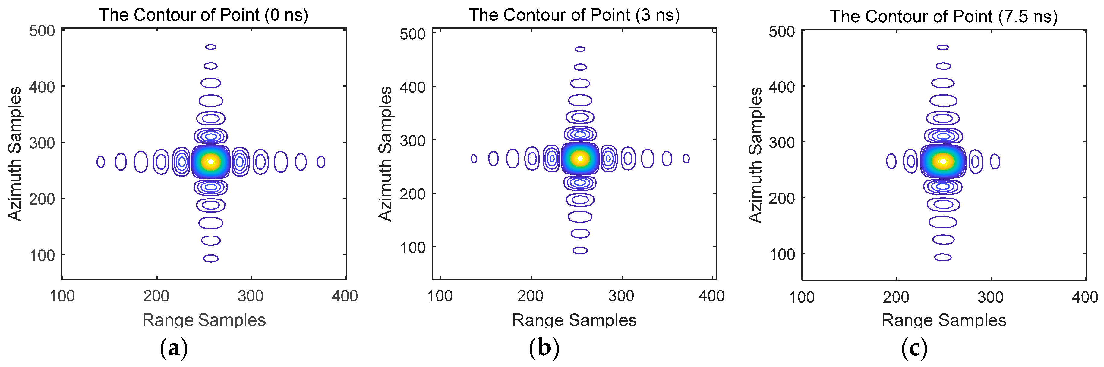
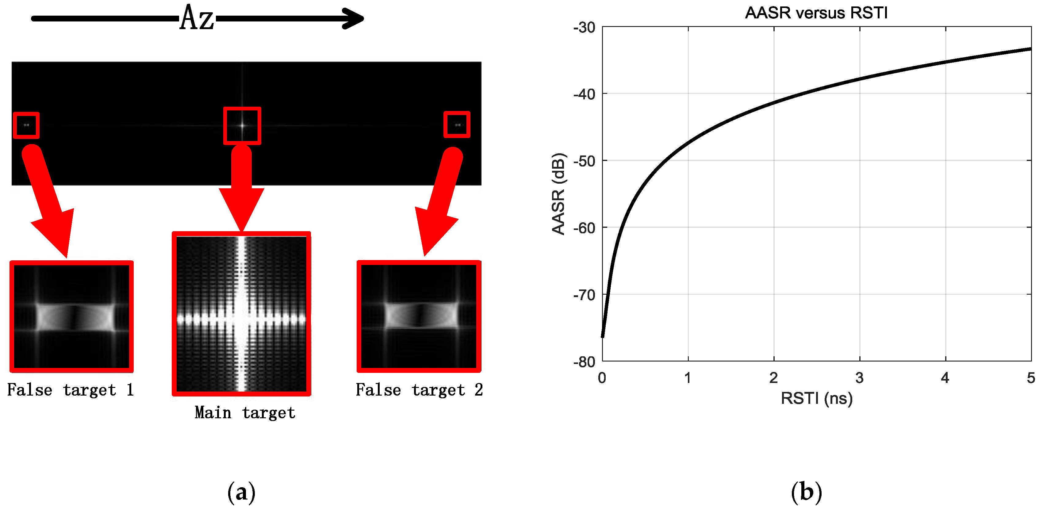
3.1. Range Sample Time Imbalance
3.2. Phase Imbalance
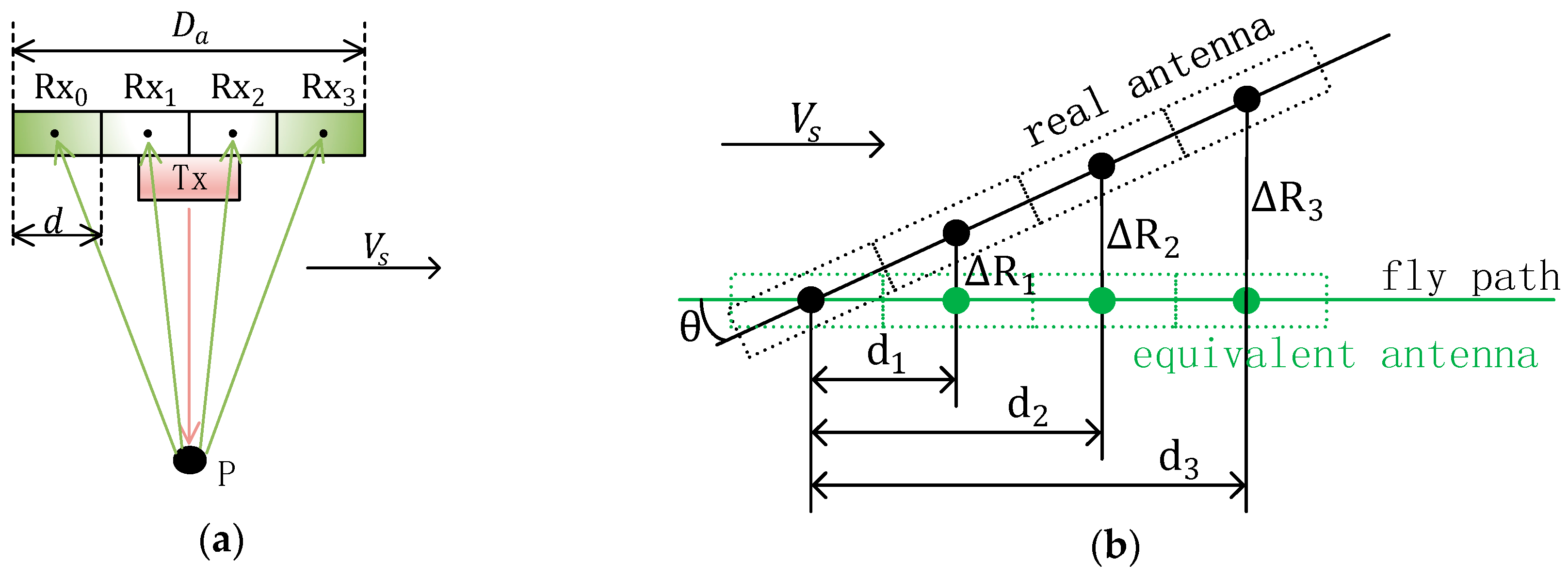
3.3. Along-Track Baseline
3.4. Processing Flow
4. Simulation and Real Data Processing
4.1. Simulation Data Processing
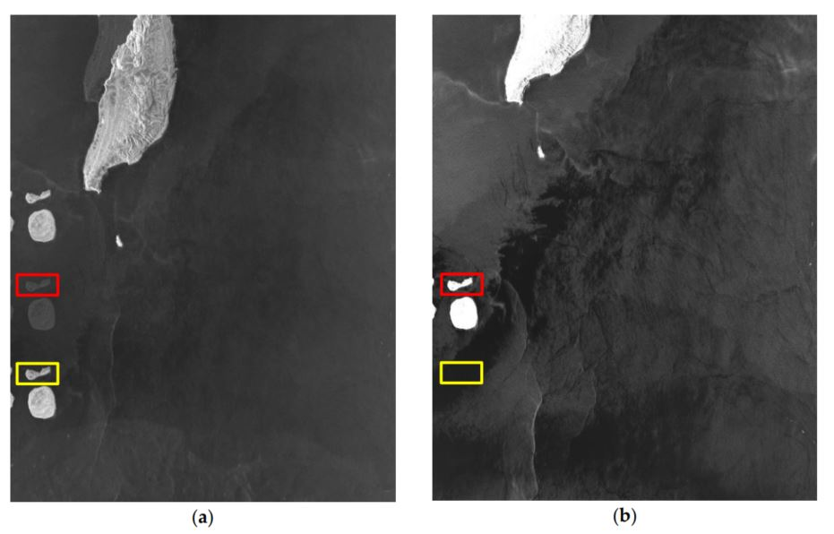
4.2. Real Data Processing
5. Discussion
6. Conclusion and Research Perspectives
Author Contributions
Funding
Acknowledgments
Conflicts of Interest
References
- Carrara, W.G.; Goodman, R.S.; Majewski, R.M. Spotlight synthetic aperture radar: Signal processing algorithms. J. Atmos. Sol. Terr. Phys. 1995, 59, 597–598. [Google Scholar]
- Tomiyasu, K. Tutorial review of synthetic-aperture radar (SAR) with applications to imaging of the ocean surface. Proc. IEEE 1978, 66, 563–583. [Google Scholar] [CrossRef]
- Suess, M.; Grafmueller, B.; Zahn, R. A novel high resolution, wide swath SAR system. In Proceedings of the IEEE 2001 International Geoscience and Remote Sensing Symposium (IGARSS ‘01), Sydney, Australia, 9–13 July 2001; Volume 3, pp. 1013–1015. [Google Scholar]
- Matar, J.; Dekker, F.L.; Krieger, G. Potentials and Limitations of MEO SAR. In Proceedings of the 11th European Conference on Synthetic Aperture Radar (Eusar 2006), Hamburg, Germany, 6–9 June 2016. [Google Scholar]
- Gerber, A.J., Jr.; Tralli, D.M.; Bajpai, S.N. Medium Earth Orbit (MEO) as an Operational Observation Venue for NOAA’s Environmental Satellites. Proc. SPIE 2005, 5659, 261–271. [Google Scholar]
- Glaser, J.I. Fifty years of bistatic and multistatic radar. IEE Proc. F Commun. Radar Signal Process. 1986, 133, 596–603. [Google Scholar] [CrossRef]
- Krieger, G.; Moreira, A. Spaceborne Bi- and Multistatic SAR: Potential and Challenges. IEE Proc. Radar Sonar Navig. 2006, 153, 184–198. [Google Scholar] [CrossRef]
- Krieger, G.; Fiedler, H.; Hounam, D.; Moreira, A. Analysis of System Concepts for Bi-and Multistatic SAR Missions. In Proceedings of the IEEE 2003 International Geoscience and Remote Sensing Symposium (IGARSS ‘03), Toulouse, France, 21–25 July 2003. [Google Scholar]
- Li, Z.; Zheng, B.; Wang, H.; Liao, G. Performance improvement for constellation SAR using signal processing techniques. IEEE Trans. Aerosp. Electron. Syst. 2006, 42, 436–452. [Google Scholar]
- Li, Z.; Bao, Z. A novel approach for wide-swath and high-resolution SAR image generation from distributed small spaceborne SAR systems. Int. J. Remote Sens. 2006, 27, 1015–1033. [Google Scholar] [CrossRef]
- Goodman, N.A.; Lin, S.C.; Rajakrishna, D.; Stiles, J.M. Processing of multiple-receiver spaceborne arrays for wide-area SAR. Geosci. Remote Sens. IEEE Trans. 2002, 40, 841–852. [Google Scholar] [CrossRef]
- Wang, W.Q. GPS-Based Time & Phase Synchronization Processing for Distributed SAR. IEEE Trans. Aerosp. Electron. Syst. 2009, 45, 1040–1051. [Google Scholar]
- Currie, A.; Brown, M.A. Wide-swath SAR. Radar Signal Process. IEE Proc. F 1992, 139, 122–135. [Google Scholar] [CrossRef]
- Li, Z.; Wang, H.; Tao, S.; Zheng, B. Generation of wide-swath and high-resolution SAR images from multichannel small spaceborne SAR systems. IEEE Geosci. Remote Sens. Lett. 2005, 2, 82–86. [Google Scholar] [CrossRef]
- Han, B.; Ding, C.; Zhong, L.; Liu, J.; Qiu, X.; Hu, Y.; Lei, B. The GF-3 SAR Data Processor. Sensors 2018, 18, 835. [Google Scholar] [CrossRef] [PubMed]
- Sun, J.; Yu, W.; Deng, Y. The SAR Payload Design and Performance for the GF-3 Mission. Sensors 2017, 17, 2419. [Google Scholar] [CrossRef] [PubMed]
- Shang, M.; Han, B.; Ding, C.; Sun, J.; Zhang, T.; Huang, L.; Meng, D. A High-Resolution SAR Focusing Experiment Based on GF-3 Staring Data. Sensors 2018, 18, 943. [Google Scholar] [CrossRef] [PubMed]
- Sun, G.; Xiang, J.; Xing, M.; Yang, J.; Guo, L. A Channel Phase Error Correction Method Based on Joint Quality Function of GF-3 SAR Dual-Channel Images. Sensors 2018, 18, 3131. [Google Scholar] [CrossRef]
- Zheng, M.; Yan, H.; Zhang, L.; Yu, W.; Deng, Y.; Wang, R. Research on Strong Clutter Suppression for Gaofen-3 Dual-Channel SAR/GMTI. Sensors 2018, 18, 978. [Google Scholar] [CrossRef]
- Wang, C.; Liao, G.; Zhang, Q. First Spaceborne SAR-GMTI Experimental Results for the Chinese Gaofen-3 Dual-Channel SAR Sensor. Sensors 2017, 17, 2683. [Google Scholar] [CrossRef]
- Jin, T.; Qiu, X.; Hu, D.; Ding, C. Unambiguous Imaging of Static Scenes and Moving Targets with the First Chinese Dual-Channel Spaceborne SAR Sensor. Sensors 2017, 17, 1709. [Google Scholar] [CrossRef]
- Krieger, G.; Gebert, N.; Moreira, A. Unambiguous SAR signal reconstruction from nonuniform displaced phase center sampling. IEEE Geosci. Remote Sens. Lett. 2004, 1, 260–264. [Google Scholar] [CrossRef]
- Fox, P.A.; Luscombe, A.P.; Thompson, A.A. RADARSAT-2 SAR modes development and utilization. Can. J. Remote Sens. 2004, 30, 258–264. [Google Scholar] [CrossRef]
- Thompson, A.A.; Luscombe, A.P.; James, K.; Fox, P. New modes and techniques of the RADARSAT-2 SAR. In Proceedings of the IEEE 2001 International Geoscience and Remote Sensing Symposium (IGARSS ‘01), Sydney, Australia, 9–13 July 2001; Volume 481, pp. 485–487. [Google Scholar]
- Luscombe, A. Image quality and calibration of RADARSAT-2. In Proceedings of the IEEE 2009 International Geoscience and Remote Sensing Symposium (IGARSS ‘09), Cape Town, South Africa, 12–17 July 2009; pp. II-757–II-760. [Google Scholar]
- Krieger, G.; Gebert, N.; Moreira, A. SAR signal reconstruction from non-uniform displaced phase centre sampling. In Proceedings of the IEEE 2004 International Geoscience and Remote Sensing Symposium (IGARSS ‘04), Anchorage, AK, USA, 20–24 September 2004; pp. 1034–1037. [Google Scholar]
- Kim, J.H.; Younis, M.; Prats-Iraola, P.; Gabele, M.; Krieger, G. First Spaceborne Demonstration of Digital Beamforming for Azimuth Ambiguity Suppression. IEEE Trans. Geosci. Remote Sens. 2013, 51, 579–590. [Google Scholar] [CrossRef]
- Werninghaus, R.; Buckreuss, S. The TerraSAR-X Mission and System Design. IEEE Trans. Geosci. Remote Sens. 2010, 48, 606–614. [Google Scholar] [CrossRef]
- Mittermayer, J.; Runge, H. Conceptual studies for exploiting the TerraSAR-X dual receive antenna. In Proceedings of the IEEE 2003 International Geoscience and Remote Sensing Symposium (IGARSS ‘03), Toulouse, France, 21–25 July 2003; pp. 2140–2142. [Google Scholar]
- Okada, Y.; Nakamura, S.; Iribe, K.; Yokota, Y.; Tsuji, M.; Tsuchida, M.; Hariu, K.; Kankaku, Y.; Suzuki, S.; Osawa, Y. System design of wide swath, high resolution, full polarimietoric L-band SAR onboard ALOS-2. In Proceedings of the IEEE 2013 International Geoscience and Remote Sensing Symposium (IGARSS 2013), Melbourne, Australia, 21–26 July 2013; pp. 2408–2411. [Google Scholar]
- Kankaku, Y.; Suzuki, S.; Osawa, Y. ALOS-2 mission and development status. In Proceedings of the IEEE 2013 International Geoscience and Remote Sensing Symposium (IGARSS 2013), Melbourne, Australia, 21–26 July 2013; pp. 2396–2399. [Google Scholar]
- Zhang, L.; Xing, M.D.; Qiu, C.W.; Bao, Z. Adaptive two-step calibration for high resolution and wide-swath SAR imaging. IET Radar Sonar Navig. 2010, 4, 548–559. [Google Scholar] [CrossRef]
- Yang, T.; Li, Z.; Liu, Y.; Bao, Z. Channel Error Estimation Methods for Multichannel SAR Systems in the azimuth. IEEE Geosci. Remote Sens. Lett. 2012, 10, 548–552. [Google Scholar] [CrossRef]
- Liu, Y.Y.; Li, Z.F.; Suo, Z.Y.; Bao, Z. A novel channel phase bias estimation method for spaceborne along-track multi-channel HRWS SAR in time-domain. In Proceedings of the IEEE 2013 International Geoscience and Remote Sensing Symposium (IGARSS 2013), Melbourne, Australia, 21–26 July 2013; pp. 1–4. [Google Scholar]
- Feng, J.; Gao, C.; Zhang, Y.; Wang, R. Phase Mismatch Calibration of the Multichannel SAR Based on Azimuth Cross Correlation. IEEE Geosci. Remote Sens. Lett. 2013, 10, 903–907. [Google Scholar] [CrossRef]
- Madsen, S.N. Estimating the Doppler centroid of SAR data. IEEE Trans. Aerosp. Electron. Syst. 1989, 25, 134–140. [Google Scholar] [CrossRef] [Green Version]
- Yang, T.; Li, Z.; Liu, Y.; Suo, Z.; Bao, Z. Channel error estimation methods for multi-channel HRWS SAR systems. In Proceedings of the IEEE 2013 International Geoscience and Remote Sensing Symposium (IGARSS 2013), Melbourne, Australia, 21–26 July 2013; pp. 4507–4510. [Google Scholar]
- Jin, T.; Qiu, X.; Hu, D.; Ding, C. Estimation Accuracy and Cramér–Rao Lower Bounds for Errors in Multichannel HRWS SAR Systems. IEEE Geosci. Remote Sens. Lett. 2016, 13, 1772–1776. [Google Scholar] [CrossRef]
- Jin, T.; Qiu, X.; Hu, D.; Ding, C. Channel Error Estimation Methods Comparison under Different Conditions for Multichannel HRWS SAR Systems. J. Comput. Commun. 2016, 4, 88–94. [Google Scholar] [CrossRef] [Green Version]
- Cumming, I.G.; Wong, F.H. Digital Signal Processing of Synthetic Aperture Radar Data: Algorithm and Implementation; Artech House: Norwood, MA, USA, 2004. [Google Scholar]
- Bamler, R. A comparison of range-Doppler and wavenumber domain SAR focusing algorithms. IEEE Trans. Geosci. Remote Sens. 1992, 30, 706–713. [Google Scholar] [CrossRef]
- Raney, R.K.; Runge, H.; Bamler, R.; Cumming, I.G.; Wong, F.H. Precision SAR processing using chirp scaling. IEEE Trans. Geosci. Remote Sens. 1994, 32, 786–799. [Google Scholar] [CrossRef]
- Stearns, S.D.; Hush, D.R. Digital Signal Analysis, 2nd ed.; Prentice Hall: Englewood Cliffs, NJ, USA, 1990. [Google Scholar]
- Brown, J.L., Jr. Multi-channel sampling of low-pass signals. IEEE Trans. Circuits Syst. 1981, 28, 101–106. [Google Scholar] [CrossRef]
- Fiedler, H.; Boerner, E.; Mittermayer, J.; Krieger, G. Total zero Doppler Steering-a new method for minimizing the Doppler centroid. IEEE Geosci. Remote Sens. Lett. 2005, 2, 141–145. [Google Scholar] [CrossRef]
- Yu, Z.; Zhou, Y.; Chen, J.; Li, C. A new satellite attitude steering approach for zero Doppler centroid. In Proceedings of the 2009 IET International Radar Conference, Guilin, China, 20–22 April 2009; pp. 1–4. [Google Scholar]
- Boerner, E.; Fiedler, H.; Krieger, G.; Mittermayer, J. A new method for Total Zero Doppler Steering. In Proceedings of the IEEE 2004 International Geoscience and Remote Sensing Symposium (IGARSS ‘04), Anchorage, AK, USA, 20–24 September 2004; Volume 1522, pp. 1526–1529. [Google Scholar]
- Mittermayer, J.; Wollstadt, S.; Prats-Iraola, P.; Scheiber, R. The TerraSAR-X Staring Spotlight Mode Concept. IEEE Trans. Geosci. Remote Sens. 2014, 52, 3695–3706. [Google Scholar] [CrossRef]
- Lanari, R.; Zoffoli, S.; Sansosti, E.; Fornaro, G.; Serafino, F. New approach for hybrid strip-map/spotlight SAR data focusing. IEE Proc. Radar Sonar Navig. 2001, 148, 363–372. [Google Scholar] [CrossRef]
- Janoth, J.; Gantert, S.; Schrage, T.; Kaptein, A. Terrasar next generation—Mission capabilities. In Proceedings of the IEEE 2013 International Geoscience and Remote Sensing Symposium (IGARSS 2013), Melbourne, Australia, 21–26 July 2013. [Google Scholar]
- Chen, S.; Huang, L.; Qiu, X.; Shang, M.; Han, B. An Improved Imaging Algorithm for High-Resolution Spotlight SAR with Continuous PRI Variation Based on Modified Sinc Interpolation. Sensors 2019, 19, 389. [Google Scholar] [CrossRef] [PubMed]
- Gebert, N.; Krieger, G.; Moreira, A. Multichannel Azimuth Processing in ScanSAR and TOPS Mode Operation. IEEE Trans. Geosci. Remote Sens. 2013, 51, 4611. [Google Scholar] [CrossRef]
- Moore, R.K.; Claassen, J.P.; Lin, Y.H. Scanning Spaceborne Synthetic Aperture Radar with Integrated Radiometer. IEEE Trans. Aerosp. Electron. Syst. 1981, AES-17, 410–421. [Google Scholar] [CrossRef]


| Parameter | Value |
|---|---|
| Channel number (M) | 2 |
| Wavelength () | 0.0556 m |
| Platform velocity () | 7571.68 m/s |
| Signal bandwidth () | 100 MHz |
| Sampling Rate | 133.33 MHz |
| PRF | 1976.93 Hz |
| Ideal PRF | 2019.12 Hz |
| Antenna length () | 7.5 m |
| Along-track baseline () | 3.75 m |
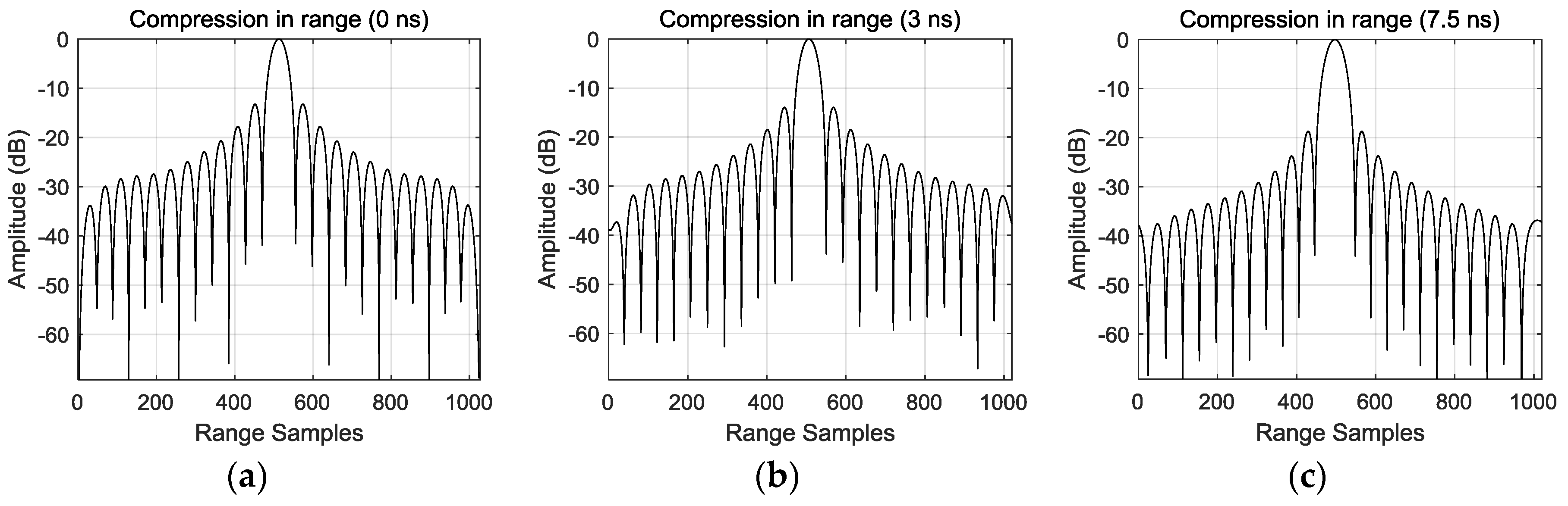
| RSTI (ns) | Max Value1 | Resolution (m) | PSLR (dB) | ISLR (dB) |
|---|---|---|---|---|
| 0.0 | 215405.79 | 1.508 | −13.263 | −10.070 |
| 3.0 | 207463.67 | 1.548 | −13.927 | −10.851 |
| 7.5 | 168900.21 | 1.667 | −18.719 | −16.626 |
| SNR (dB) | RSTI (ns) | Phase Imbalance (°) | Along-Track Baseline (m) |
|---|---|---|---|
| 0 | 7.0456 | 19.5255 | 3.6944 |
| 5 | 7.2120 | 20.2442 | 3.7340 |
| 10 | 7.4017 | 19.7183 | 3.7524 |
| 15 | 7.4342 | 19.6788 | 3.7506 |
| 20 | 7.4621 | 19.9009 | 3.7502 |
| Estimated Value | |
|---|---|
| RSTI (ns) | 0.218 |
| Phase Imbalance (°) | −167.541 |
| Along-track baseline (m) | 3.681 |
© 2019 by the authors. Licensee MDPI, Basel, Switzerland. This article is an open access article distributed under the terms and conditions of the Creative Commons Attribution (CC BY) license (http://creativecommons.org/licenses/by/4.0/).
Share and Cite
Shang, M.; Qiu, X.; Han, B.; Ding, C.; Hu, Y. Channel Imbalances and Along-Track Baseline Estimation for the GF-3 Azimuth Multichannel Mode. Remote Sens. 2019, 11, 1297. https://doi.org/10.3390/rs11111297
Shang M, Qiu X, Han B, Ding C, Hu Y. Channel Imbalances and Along-Track Baseline Estimation for the GF-3 Azimuth Multichannel Mode. Remote Sensing. 2019; 11(11):1297. https://doi.org/10.3390/rs11111297
Chicago/Turabian StyleShang, Mingyang, Xiaolan Qiu, Bing Han, Chibiao Ding, and Yuxin Hu. 2019. "Channel Imbalances and Along-Track Baseline Estimation for the GF-3 Azimuth Multichannel Mode" Remote Sensing 11, no. 11: 1297. https://doi.org/10.3390/rs11111297
APA StyleShang, M., Qiu, X., Han, B., Ding, C., & Hu, Y. (2019). Channel Imbalances and Along-Track Baseline Estimation for the GF-3 Azimuth Multichannel Mode. Remote Sensing, 11(11), 1297. https://doi.org/10.3390/rs11111297