Probability Index of Low Stratus and Fog at Dawn using Dual Geostationary Satellite Observations from COMS and FY-2D near the Korean Peninsula

Abstract

We developed a new remote sensing method for detecting low stratus and fog (LSF) at dawn in terms of probability index (PI) of LSF from simultaneous stereo observations of two geostationary-orbit satellites; the Korean Communication, Ocean, and Meteorological Satellite (COMS; 128.2°E); and the Chinese FengYun satellite (FY-2D; 86.5°E). The algorithm was validated near the Korean Peninsula between the months of April and August from April 2012 to June 2015, by using surface observations at 45 meteorological stations in South Korea. The optical features of LSF were estimated by using satellite retrievals and simulated data from the radiative transfer model. The PI was calculated using the combination of three satellite-observed variables: 1) the reflectance at 0.67 μm (R_0.67) from COMS, and 2) the FY-2D R_0.67 minus the COMS R_0.67 (△R_0.67) and 3) the FY-2D-COMS difference in the brightness temperature difference between 3.7 and 11.0 μm (ΔBTD_3.7-11). The three variables, adopted from the top three probability of detection (POD) scores for their fog detection thresholds: △R_0.67 (0.82) > ΔBTD_3.7-11 (0.73) > R_0.67 (0.70) > BTD_3.7-11 (0.51). The LSF PI for this algorithm was significantly better in the two case studies compared to that using COMS only (i.e., R_0.67 or BTD_3.7-11), so that this improvement was due to △R_0.67 and ΔBTD_3.7-11. Overall, PI in the LSF spatial distribution has the merits of a high detection rate, a specific probability display, and a low rate of seasonality and variability in detection accuracy. Therefore, PI would be useful for monitoring LSF in near-real-time, and to further its forecast ability, using next-generation satellites.

1. Introduction

Improved sensing of low stratus and fog (LSF) has important implications for safety in ground, sea, and air transportation, because of reduced visibility [1]. Fog occurs frequently in South Korea, particularly during the dawn and dusk rush hours, so that accurate fog detection is of vital importance in risk management, to reduce potential life and economic losses. Ground-based and satellite-based observations are commonly used for fog detection. The accuracy of ground-based observations by the naked-eye is high (80.8%), and is at 70.5% using a visibility meter [2]. However, the range is mostly limited to inland and coastal areas (or islands), making it difficult to monitor fog over larger areas, such as the open sea [3,4]. To supplement the spatial limit of ground-based observations, satellite-based fog sensing can be introduced, since it is capable of providing a spatially uniform dataset over a wide area. As the LSF sensing methods from satellite observations only have fundamental difficulties in distinguishing between low stratus and fog [5], most previous studies have used the integrated terminology of either LSF or fog and low stratus (FLS) without explicitly separating the types [2,3,6,7,8,9,10]. For example, the spatial and temporal gaps that are undetected by the ground-based LSF observations have been filled by the Moderate Resolution Imaging Spectroradiometer (MODIS) or the Advanced Very High Resolution Radiometer (AVHRR) [11,12]. With these sun-synchronized satellites, however, monitoring LSF remains limited to only once a day.

Thus, observations from geostationary-orbit satellites (GEOs) are suitable for detecting and predicting fog, because they can trace the evolution of advective fog all day long. The spatial resolution of GEOs has substantially improved, and it is suitable for detecting LSF on 1–5 km spatial resolutions. Cermak and Bendix [13] developed the LSF detection scheme, using the Spinning Enhanced Visible and Infrared Imager (SEVIRI) data onboard the Meteosat Second Generation (MSG) GEOs during the winter months of 2004–2008, with a sequence of threshold tests, using different wavelength bands. Their original algorithms were chosen by Egli et al. [2] for use in various spatiotemporal conditions. The LSF information is derived from empirical thresholds after removing atmospheric signals from satellite observations. The thresholds are statistically obtained from the frequency distributions of the observations (i.e., the brightness temperature or visible reflectance of specified wavelengths) on the LSF layer, possibly in the absence of higher clouds. The thresholds for the infrared brightness temperature difference (BTD_3.7–11) and the visible reflectance (R_0.67) at daytime or BTD_3.7-11 at nighttime have been used in previous GEO-related studies [14,15,16]. BTD_3.7–11 results from the fact that the emissivity for water particles in the shortwave infrared (SWIR) brightness temperature at 3.7 μm (i.e., BT_3.7) is significantly less than in the infrared brightness temperature at 11 μm (i.e., BT₁₁) (e.g., [11,17,18]). However, LSF detection at dawn and dusk has not been successful, due to the reduced signal-to-noise (SNR) ratio of visible reflectance (R_0.67), in association with weak solar radiation or negligible emissivity.

To overcome the drawback of R_0.67, some studies have suggested the use of different channels in GEOs or the surface temperature information. The Korea Meteorological Administration [19] has conducted daytime and nighttime fog detection observations near the Korean Peninsula, utilizing Korean Communication, Ocean, and Meteorological Satellite (COMS) data since the satellite was launched in June 2010. KMA [19] utilized the COMS L1b data to calculate the fog-related output every 15 minutes, based on the operational fog detection algorithm of the meteorological data processing system. The algorithm performed the other threshold tests for removing cloud contamination before applying the fog-detection thresholds to the satellite observations. The cloud contamination in the algorithm was removed by checking the BTD thresholds between the window channel at 11 μm (IR1) and the water vapor channel at ~6.7 μm (i.e., BTD_11−6.7) and between IR1 and the infrared channel at 12.0 μm (IR2). The ground temperature was used for additional information.

Kim et al. [20], and Shin and Kim [21] used satellite observations (COMS or Himawari-8) for nighttime fog detection in the region, in conjunction with additional land and sea surface temperature information. Although the BTD_3.7-11 threshold is expected to be more useful for night observations rather than dawn and dusk, the detection in their studies [20,21] was inaccurate (false alarm ratio; FAR = 0.43 − 0.56) and requires additional information (e.g., multiple satellite observations, more independent channels) for improvement. The inaccuracy may also be due to uncertainties caused by using land/sea surface temperatures as low boundary conditions, and the presence of higher clouds [22]. KMA [23] also attempted a ‘dynamic threshold value’ method to detect LSF at dawn and dusk (SZA ≥ 60°), which used the different threshold values at each scene [24,25,26]. However, this method was unable to essentially improve the fog detection at the time zone, because of the SNR limitation [8]. Indeed, most of the single-satellite LSF sensing methods was inaccurate at sunrise in previous studies [26,27,28].

Recently, Yoo et al. [8] showed that the so-called dual-satellite method (DSM) could be useful for LSF detection at dawn. DSM uses two different satellite images observed from different viewing angles, so that the SNR of LSF can be amplified. Using almost simultaneous stereo observations near the Korean Peninsula from the FY-2D and COMS GEOs, the use of the difference in R_0.67 between the two satellites, in addition to the R_0.67 of COMS was found to greatly improve the LSF detection skills. However, the merits of DSM were limited to detection in summer only (June to August) [8].

By improving the DSM of Yoo et al. [8], this study attempts to develop the probability index (PI) of LSF, in order to provide the possibility of fog occurrences spatially in the weather map. First, we applied DSM to the infrared channels, so that DSM is applicable to a more extended warm period (April to August). This is because the seasonality is weaker in the infrared channels than in the visible channels, based on the bidirectional reflectance distribution function (BRDF; Figure 9 of Yoo et al. [8]). The strong seasonality was a main reason for why the visible information in [8] was not applied to other seasons than summer. Radiative Transfer Model (RTM)-simulated results are also used for insights into the satellite retrievals and the LSF optical characteristics. Satellite- and ground-based observations, PI formulation, and LSF retrieval schemes are described in Section 2. A case study for fog occurrences, using satellite observations and RTM simulation, is described in Section 3. The derivation and verification of the optimum threshold are presented in this section. While our focus is on developing LSF PI, the improved level of LSF detection is also explained and compared to those from other operational algorithms.

2. Materials and Methods

The near-simultaneous observations of the dual satellites (COMS and FY-2D) for the LSF detection at dawn near the Korean Peninsula are defined as the differences between their stereoscopic views. For this study’s purpose, ‘dawn’ is within two hours after sunrise (67° < SZA < 86°). Ground-based fog observations and associated numerical experiments were used to validate the satellite-derived LSF detections.

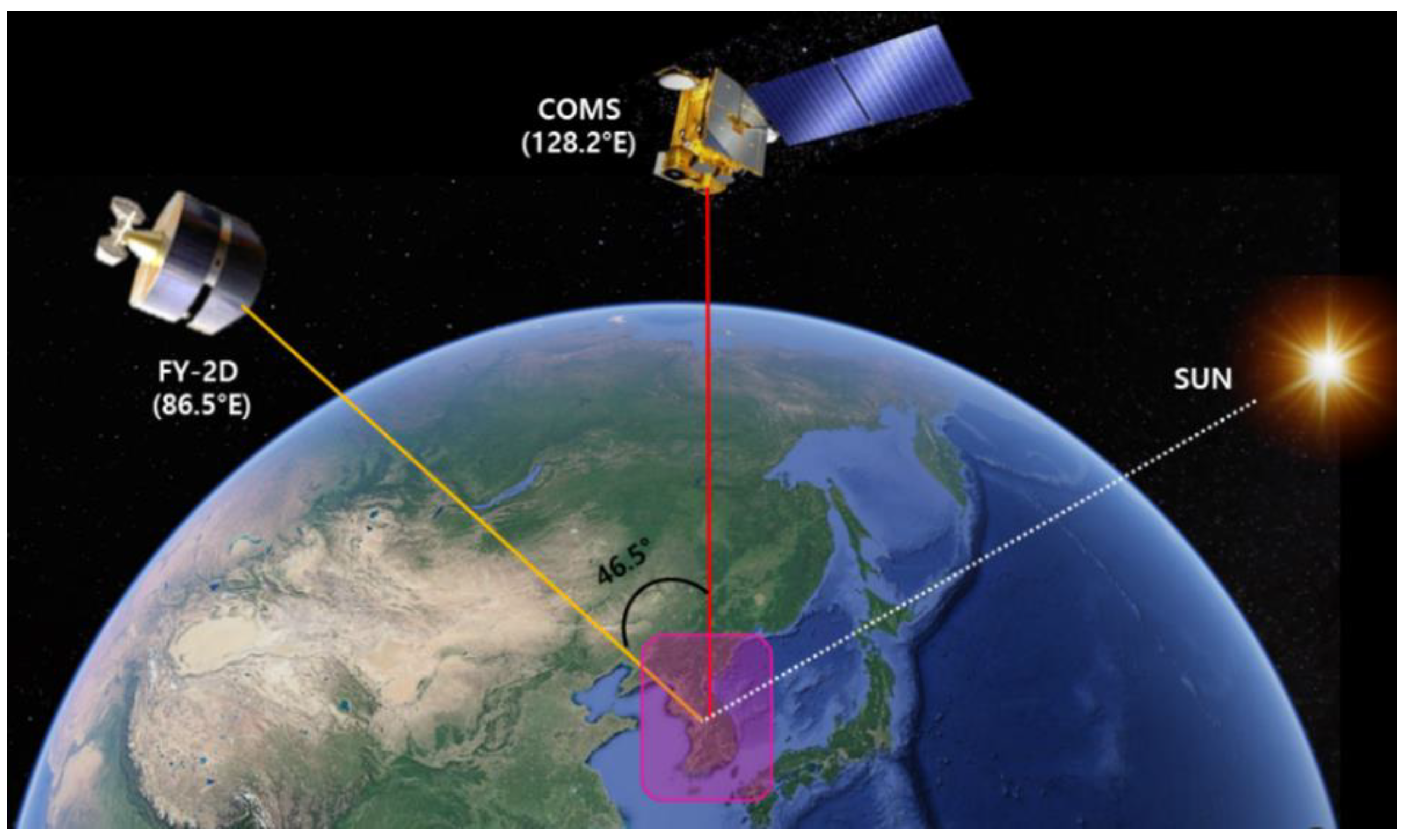
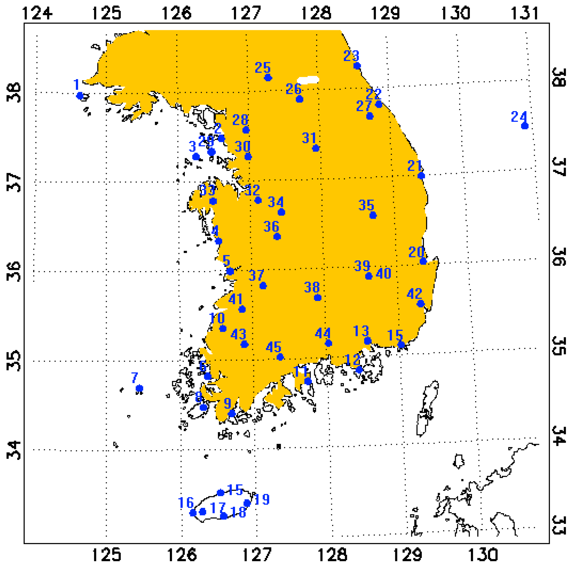
2.1. Satellite and Ground-Based Observations

The data from three channels (R_0.67, BT_3.7, and BT₁₁) in each satellite were utilized for the LSF detection. The satellite information is summarized in

Table 1. Information about the COMS and FY-2D dual geostationary satellites used in the nearly-simultaneous observations of low stratus and fog near the Korean Peninsula [29,30]. Please see Table A1 for the acronyms.

Satellite	Longitude (°E)	Altitude (km)	Launch Date	VIS (μm)	SWIR (μm)	IR1 (μm)	Central Wavelength (μm)	Spatial Resolution (km)
COMS	128.2	35,857	27 Jun 2010	0.55–0.80	3.5–4.0	10.3–11.3	0.675/3.75/10.8	1/4/4
FY-2D	86.5	35,786	15 Nov 2006	0.55–0.99	3.5–4.0	10.3–11.3	0.77/3.75/10.8	1.25/5/5

, and their locations are shown in Figure 1. The COMS data were linearly interpolated onto the FY-2D dataset for comparison at the same spatial resolutions. The maximum time difference allowed between COMS and FY-2D observations for this study was 15 minutes. We derived R_0.67, BTD_3.7-11, ΔR_0.67, and ΔBTD_3.7-11 from these datasets. The differences in R_0.67 and BTD_3.7-11 between the satellites can be defined as follows:

$$\Delta {\mathrm{R}}_{0.67}={\mathrm{R}}_{\mathrm{FY}-2\mathrm{D}}-{\mathrm{R}}_{\mathrm{COMS}}$$

(1)

$$\Delta {\mathrm{BTD}}_{3.7-11}={\mathrm{BTD}}_{\mathrm{FY}-2\mathrm{D}}-{\mathrm{BTD}}_{\mathrm{COMS}}$$

(2)

Here, ${\mathrm{R}}_{\mathrm{FY}-2\mathrm{D}}$ and ${\mathrm{R}}_{\mathrm{COMS}}$ are the R_0.67 values of the FY-2D and COMS satellites, respectively. Similarly, ${\mathrm{BTD}}_{\mathrm{FY}-2\mathrm{D}}$ and ${\mathrm{BTD}}_{\mathrm{COMS}}$ are the BTD_3.7-11 values of the corresponding satellites. The ΔR_0.67 threshold for LSF detection from the dual satellites in [8] was shown to be superior to the existing R_0.67 and BTD_3.7-11 thresholds of the COMS satellite alone. In our study, we introduce ΔBTD_3.7-11 as an additional variable to improve the spring (April and May) and summer LSF detection accuracy. The dual satellite observations (i.e., ΔR_0.67 and ΔBTD_3.7-11), as well as R_0.67, are utilized as three components in the PI formulation. This provides a more accurate detection and specific display for the weather phenomenon, than the individual thresholds described in previous studies (e.g., [8,19]). It is because the ΔBTD_3.7-11 in (2) has less seasonality in the LSF detection than the ΔR_0.67 in (1), and because it is useful, particularly in April–May, over the Yellow Sea [31]. The R_0.67 values of less than 0.001 were excluded in the process of data quality control in this study.

Ground-based fog and clear-sky observations [32] were used to derive and validate PI for LSF detection at dawn in South Korea from April to August between April 2012 and June 2015. There are 45 meteorological ground stations located in the country’s inland and coastal regions (Figure 2 and

Table A2. The 45 meteorological stations in South Korea used in the LSF analysis.

Station Number	Coastal Station	Lat (°N)	Lon (°E)	Height (m)	Station Number	Inland Station	Lat (°N)	Lon (°E)	Height (m)
1	Baengnyeongdo	37.97	124.63	145	24	Ulleungdo	37.48	130.90	223
2	Incheon	37.48	126.62	68	25	Cheorwon	38.15	127.30	154
3	Incheon Airport	37.28	126.26	N/A	26	Chuncheon	37.90	127.74	78
4	Boryeong	36.33	126.56	15	27	Daeguallyeong	37.68	128.72	773
5	Gunsan	35.99	126.71	26	28	Seoul	37.57	126.97	86
6	Mokpo	34.82	126.38	38	29	Gimpo Airport	37.33	126.48	N/A
7	Heuksando	34.69	125.45	76	30	Suwon	37.27	126.99	34
8	Jindo	34.47	126.32	476	31	Wonju	37.34	127.95	149
9	Wando	34.40	126.70	35	32	Cheonan	36.78	127.12	21
10	Gochang	35.35	126.60	52	33	Seosan	36.78	126.49	29
11	Yeosu	34.74	127.74	65	34	Cheongju	36.64	127.44	57
12	Tongyeong	34.85	128.44	33	35	Andong	36.57	128.71	139
13	Changwon	35.17	128.57	37	36	Daejeon	36.37	127.37	69
15	Busan	35.11	129.03	70	37	Jeonju	35.82	127.16	53
15	Jeju	33.51	126.53	20	38	Geochang	35.67	127.91	226
16	Gosan	33.29	126.16	74	39	Daegu	35.89	128.62	64
17	Jeju Airport	33.30	126.29	N/A	40	Daegu(kma)	35.89	128.62	64
18	Seogwipo	33.25	126.57	50	41	Jeongeup	35.56	126.87	45
19	Seongsan	33.39	126.88	18	42	Ulsan	35.56	129.32	35
20	Pohang	36.03	129.38	2	43	Gwangju	35.17	126.89	72
21	Uljin	36.99	129.41	50	44	Jinju	35.16	128.04	30
22	Bukgangneung	37.81	128.86	79	45	Suncheon	35.02	127.37	165
23	Sokcho	38.25	128.57	18

). Ground observations included data on the cloud amount, visibility, rain, and mist at a one-hour interval. In most cases, visibility and cloud altitude are determined by an automatic weather system, but some stations still operate by utilizing human observers. A total of 754 fog and 433 clear-sky cases from the ground-based observations were used to derive the LSF thresholds and the PI for the detection (

Table 2. Ground-based fog and clear-sky observations used to validate the probability index (PI) for the LSF detection at dawn at 45 meteorological stations in South Korea.

Weather Phenomenon	Spring (April–May)		Summer (June–August)		Dry Season (September–April)		Total Number of Observations
	Period 1	Period 2	Period 1	Period 2	Period 1	Period 2
Fog	183	138	287	146			754
Clear-sky (cloud amount≤ 10%)					255	178	433

). The fog and clear-sky data were subdivided into two periods, control data during 2012–2013 and experimental data during 2014–2015. Relatively optically thick fog cases were investigated in this study. Therefore, fog cases with a duration of at least 30 minutes were selected to exclude optically thin fog cases. The clear-sky, in contrast with the fog, was defined in this study as a cloud amount of less than 10% during the dry period (i.e., September to April). These months were chosen because clear-sky occurrences are rare between May and August, due to persistent rain and yellow dust, possibly resulting in cloud or aerosol contamination. In order to compare satellite-derived higher cloud classifications above the LSF layer with the ground-based observations, the cloud type and height data from the reports of both ground stations and surface synoptic observations (SYNOP) were used [33]. Cloud-type data were often described as being ‘missing’ or omitted from the reports, especially for middle and high clouds. The ‘missing’ cases were excluded in this study.

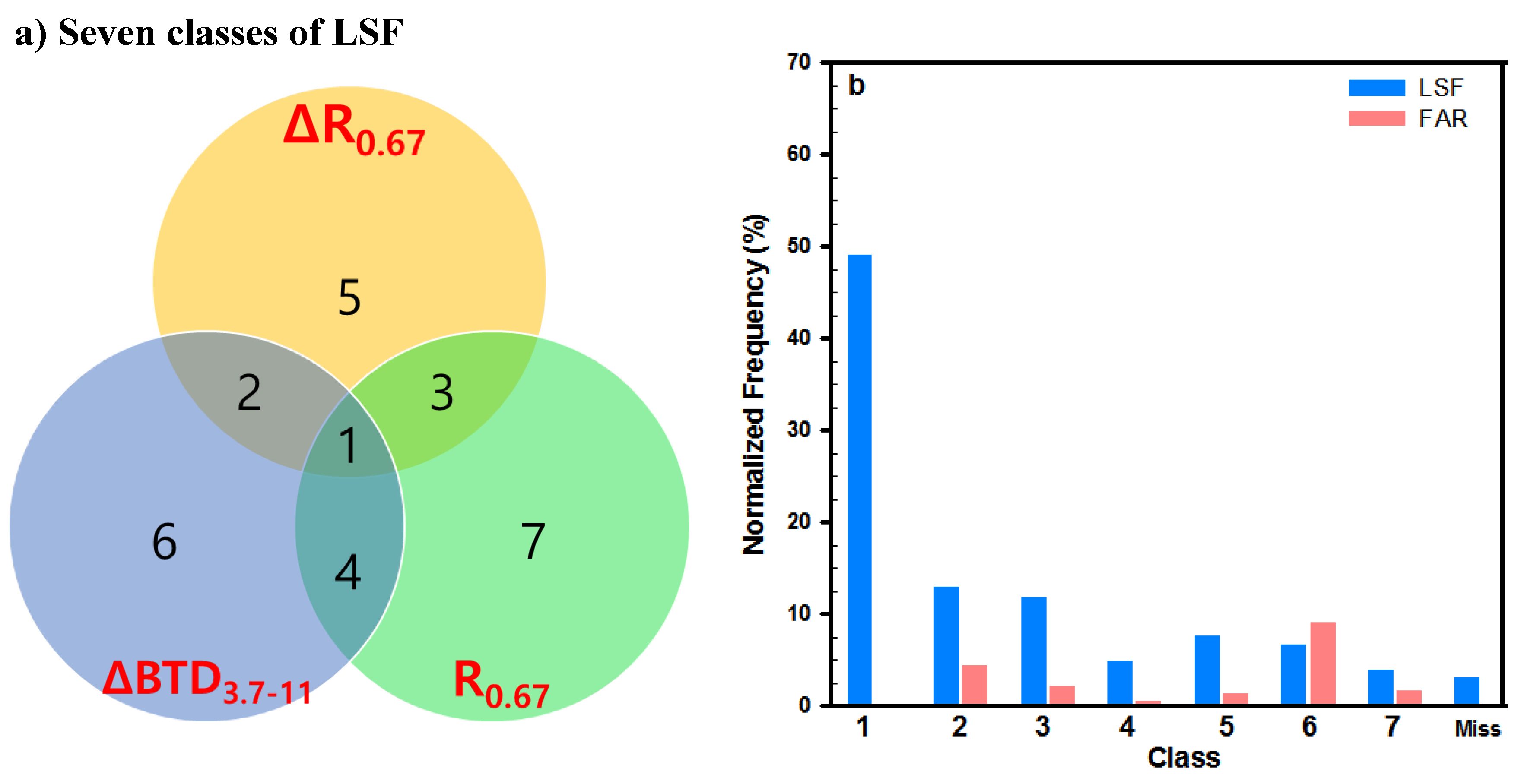
2.2. Probability Index Formulation from Past Fog Observations

The PI formulation converts the long-term LSF probabilities to the near real-time LSF probabilities. To make the long-term LSF probabilities, we have counted the frequencies of LSF occurrences in a grid for the 18 months. The LSF occurrences are those detected by the three threshold tests: ΔR_0.67, ΔBTD_3.7-11, and R_0.67. Observations of ΔR_0.67 and ΔBTD_3.7-11 are taken from the two-satellites that are collocated in ~5 km $\times$ ~5 km grids, while R_0.67 from the COMS satellite pixels. As we will show later, these three tests have been selected, as they make higher probability of detection (POD) scores in LSF detection than other tests.

Seven LSF classes have been divided from a combination of the three threshold tests (Figure 3a). Each class has a long-term probability of fog detection at the 45 stations, as indicated by the frequency of each fog class, normalized by the total frequency (Figure 3b). Data from 754 fog and 433 clear-sky observations have been used for this calculation. Using the higher cloud criteria, the fog data have been categorized into two types of LSF cases (473 LSF1 and 281 LSF_highclouds, refer to

Table A1. List of acronyms used in this study.

Acronyms	Original Words (or Details)	Acronyms	Original Words (or Details)
AVHRR	Advanced Very High Resolution Radiometer	KMA	Korea meteorological administration
BT11	brightness temperature at ~11 μm	LSF	low stratus and fog
BT11max	maximum value of BT11 over the region (122–132°E, 32.5–42.5°N)	LUT	look-up table
BT3.7	brightness temperature at ~3.7 μm	MODIS	Moderate Resolution Imaging Spectroradiometer
BTD	brightness temperature difference	NFL	normalized frequency of LSF
BTD11-6.7	brightness temperature difference between 11 μm and 6.7 μm	OBS	observation
BTD3.7-11	difference between BT3.7 and BT11	PC	percentage correct
BTD6.2-11	difference between BT6.2 and BT11	PI	probability index
BTDKMA	threshold for fog detection used at KMA (2012)	POD	probability of detection
CER	cloud effective radius	R0.67	reflectance at ~0.67 μm
CH	cloud height	RAA	relative azimuth angle
COMS	Korean Communication, Ocean and Meteorological Satellite	RKMA	threshold for fog detection used at KMA (2012)
COT	cloud optical thickness	Rmin	minimum value of R0.67 over the region (122–132°E, 32.5–42.5°N)
CSI	critical success index	RTM	radiative transfer model
DSM	dual satellite method	SBDART	Santa Barbara DISORT Atmospheric Radiative Transfer
ER	effective radius	SEVIRI	Spinning Enhanced Visible and Infrared Imager
FAR	false alarm ratio	SNR	signal-to-noise
FER	fog effective radius	SRF	spectral response function
FH	fog height	SWIR	shortwave infrared at ~3.7 μm
FOT	fog optical thickness	SYNOP	surface synoptic observations
FY-2D	Chinese FengYun-2D	SZA	solar zenith angle
GEO	geostationary-orbit satellite	VZA	satellite viewing zenith angle
GTS	global telecommunications system	VIS	visible
HR	hit rate	ΔR0.67	difference in R0.67 between two satellites
HSS	Heidke skill score	ΔBTD3.7-11	difference in BTD3.7-11 between two satellites
IR1	infrared at ~11 μm	${\sigma }_{T_{11}}$	standard deviation at BT11 over the 3 × 3 grid-pixel area
IR2	infrared at ~12 μm

for the acronyms and Figure A1 for the detailed meaning). Since the three tests are not entirely independent of each other in their optical properties for detection, their information is partially overlapped. For instance, the ‘Class 1’ indicates the fog occurrences detected by the all three threshold tests. Each class provides information on the normalized frequency that is succeeded by the threshold tests (Figure 3b). In Figure 3b, there is no FAR for Class 1. For instances, Class 2 and Class 5 successfully detected fog by using the two tests (ΔR_0.67 and ΔBTD_3.7-11) and only the R_0.67 test, respectively. The LSF cases that failed the threshold tests are indicated by ‘Miss’. The Normalized Frequency of LSF (NFL) in Figure 3b is summarized in

Table 3. Normalized Frequency of LSF (NFL) and weighting factor (WF) values for each class of the DSM. The terms ‘NFL’ and ‘WF’ are defined in the text. ‘WF*’ has been obtained from the frequency ratio of fog cases to the whole data (i.e., fog and clear-sky) to include the false alarm rate (FAR) effect.

	Class							Miss	Total
	1	2	3	4	5	6	7
NFL (%) of LSF	49.07	13.00	11.80	4.91	7.69	6.63	3.85	3.05	100
NFL (%) of clear-sky	0.23	4.38	2.08	0.46	1.39	9.01	1.62	80.83	100
WF	1.00	0.90	0.80	0.70	0.60	0.50	0.50	0.00
WF*	1.00	0.84	0.91	0.95	0.91	0.56	0.81	0.06

.

With the same 18-month fog records, we estimated PI (PI^est) to be equivalent to the POD values (0.816 ± 0.02 for total LSF) of the best threshold test using ΔR_0.67 (later shown in

Table 4. Statistical verification of the six threshold values for LSF detection at dawn, using the FY-2D and COMS satellites. The values in parentheses below the LSF scores indicate the verification scores for LSF1 without the overlying higher clouds. The scores are presented for Period 1 (2012–2013), Period 2 (2014–2015), and the entire time period (2012–2015), respectively. The contingency table and definition are shown in Table A3.

Satellite-Derived Threshold	Period	LSF (LSF1)
		HSS	CSI	POD	PC	FAR
FY-2D minus COMS (ΔR0.67) 0.44 < ΔR0.67 < 0.995	2012–2013	0.673 (0.821)	0.766 (0.846)	0.802 (0.909)	0.841 (0.911)	0.055 (0.076)
	2014–2015	0.739 (0.814)	0.801 (0.826)	0.838 (0.887)	0.872 (0.907)	0.052 (0.077)
	2012–2015	0.699 (0.819)	0.780 (0.839)	0.816 (0.901)	0.853 (0.910)	0.054 (0.076)
COMS R0.67 0.185 < R0.67 < 0.529	2012–2013	0.581 (0.661)	0.670 (0.684)	0.677 (0.696)	0.783 (0.828)	0.016 (0.024)
	2014–2015	0.601 (0.701)	0.690 (0.725)	0.729(0.791)	0.799 (0.851)	0.072 (0.103)
	2012–2015	0.588 (0.676)	0.677 (0.700)	0.696(0.732)	0.789 (0.837)	0.039 (0.057)
COMS R0.67 (KMA) 0.25 < RKMA < 0.55	2012–2013	0.468 (0.494)	0.555 (0.514)	0.555 (0.514)	0.712 (0.739)	0.000 (0.000)
	2014–2015	0.525 (0.588)	0.596 (0.594)	0.602 (0.605)	0.749 (0.794)	0.017 (0.027)
	2012–2015	0.489 (0.530)	0.571 (0.544)	0.573 (0.548)	0.726 (0.761)	0.007 (0.012)
FY-2D minus COMS (ΔBTD3.7-11) 10.5K < ΔBTD3.7-11 < 34.0K	2012–2013	0.574 (0.613)	0.680 (0.656)	0.706 (0.696)	0.785 (0.804)	0.051 (0.080)
	2014–2015	0.605 (0.679)	0.709 (0.718)	0.771 (0.819)	0.805 (0.839)	0.103 (0.147)
	2012–2015	0.585 (0.638)	0.691 (0.680)	0.731 (0.742)	0.793 (0.818)	0.072 (0.109)
COMS BTD3.7-11 4.5K < BTD3.7-11 <3 1.0K	2012–2013	0.349 (0.201)	0.480 (0.277)	0.502 (0.297)	0.647 (0.583)	0.085 (0.200)
	2014–2015	0.399 (0.317)	0.495 (0.356)	0.514 (0.379)	0.678 (0.659)	0.070 (0.141)
	2012–2015	0.369 (0.245)	0.485 (0.306)	0.507 (0.328)	0.659 (0.613)	0.080 (0.176)
COMS BTD3.7-11 (KMA) 15K < BTDKMA < 50K	2012–2013	0.106 (0.016)	0.145 (0.017)	0.145 (0.017)	0.446 (0.472)	0.000 (0.000)
	2014–2015	0.101 (0.006)	0.136 (0.017)	0.137 (0.017)	0.465 (0.504)	0.049 (0.400)
	2012–2015	0.104 (0.012)	0.142 (0.017)	0. 142 (0.017)	0.453 (0.485)	0.018 (0.200)

). This is because the PI^est is PI that is estimated for the upper-limit condition of LSF detection accuracy, and it should not exceed the maximum POD value. The condition is assumed conservatively, to prevent excessive PI values. Since each threshold test has an inherently independent portion for LSF detection, the PI value (which has comprehensively been obtained from the three tests) would be better than the POD from one threshold test. Finally, the seven weighting factors ($\mathrm{WF}\left({\mathrm{Class}}_{\mathrm{i}}\right)$) in the PI formulation have to be determined, in order to satisfy the following relation:

$${\displaystyle \sum }_{\mathrm{i}=1}^7\mathrm{WF}\left({\mathrm{Class}}_{\mathrm{i}}\right)·{\mathrm{NFL}}_{\mathrm{i}}={\mathrm{PI}}^{\mathrm{est}}$$

(3)

where $\mathrm{WF}\left({\mathrm{Class}}_{\mathrm{i}}\right)$ is the weighting factor; subscript ‘$\mathrm{i}$’ is the ith class of LSF ($\mathrm{i}$ = 1 to 7); ${\mathrm{NFL}}_{\mathrm{i}}$ and ${\mathrm{PI}}^{\mathrm{est}}$ are pre-calculated values by the 18-month fog records. LSF ‘Miss’ could be considered as an eighth class, although it was not included in (3).

The WF(Class_i) values were determined, considering the three priority conditions: a high POD ranking (ΔR_0.67 > ΔBTD_3.7-11 > R_0.67) based on observations from 45 stations, common detection from two or more threshold tests, and low FAR. Table 3 shows that the $\mathrm{WF}\left({\mathrm{Class}}_{\mathrm{i}}\right)$ for seven classes ranges from 0.5 to 1. $\mathrm{WF}\left({\mathrm{Class}}_{\mathrm{i}}\right)$ for ‘Miss’ is zero. Since the $\mathrm{WF}\left({\mathrm{Class}}_{\mathrm{i}}\right)$ is related to fog detection from at least one of the three thresholds, it is assumed to be greater than ~0.5, in view of a reasonable probability of detection. Thus, the lowest WF is set to 0.5 (Table 3). The values of ‘NFL of clear-sky’ and ‘WF*’ have also been presented in the table, to analyze the clear-sky (or FAR) effect on LSF detection. The effect does not exceed 10% in each class. Also, the WF* (i.e., PI), which includes the effect, is higher in each class than 0.55. However, the effect is likely to increase over the real-time satellite scene, due to various weather conditions (e.g., clear-sky, overcast, and fog, etc.).

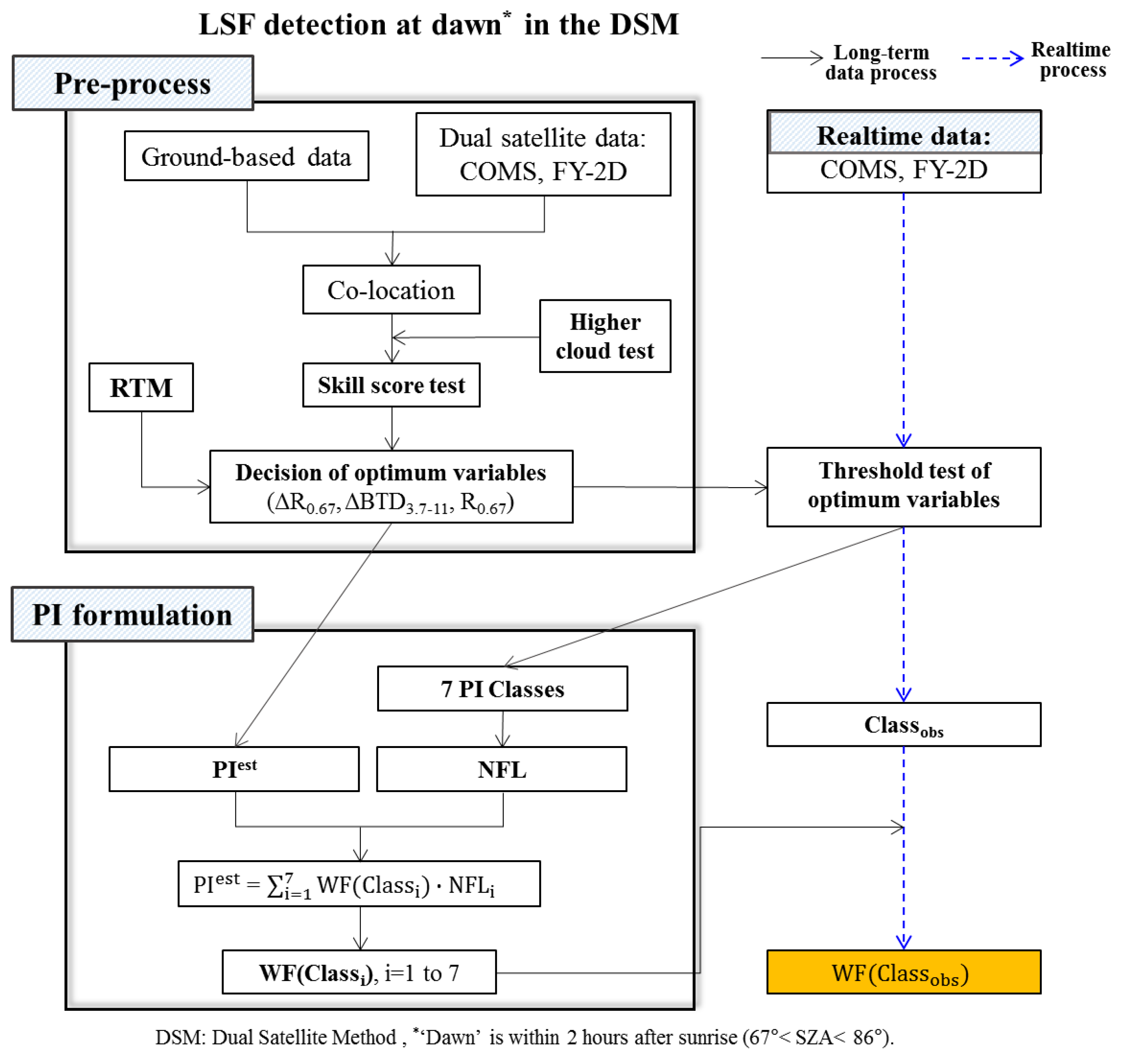
2.3. The Near-Realtime LSF PI Retrieval Scheme

The flowchart shows the entire PI calculation process for the LSF PI retrieval at dawn, using the DSM (Figure 4). It begins with the pre-process reading data (Section 2.1) and then it requires the PI formulation (Section 2.2). In the pre-process, we collocated 45 ground station sites onto ~5 km $\times$ 5 km satellite observation grids, and satellite data were collected when fog occurred at the ground stations. The optimum thresholds were derived from this information, to discriminate between fog and clear-sky cases, based on the skill score test of the variables (ΔR_0.67, R_0.67, and ΔBTD_3.7-11).

The pre-process also minimizes the effects of the higher clouds above a fog layer on the satellite-derived LSF PI retrieval. By these means, we performed RTM simulations to constructed a look-up table (LUT) for the three variables (ΔR_0.67, ΔBTD_3.7-11, and R_0.67). The RTM of the Santa Barbara DISORT Atmospheric Radiative Transfer (SBDART) was used to compute the plane-parallel radiative transfer for clear and cloudy conditions in the atmosphere and at the surface [34]. The RTM of SBDART was utilized to derive the thresholds for the fog detection and its optical characteristics for daytime [35] and nighttime [4], and at dawn [8]. The initial conditions for the RTM input were various degrees of cloudiness (i.e., clear-sky, LSF1, and LSF_highclouds) and cloud optical properties (phase, size, and optical thickness). LSF1 can be defined as being either fog or low stratus, while LSF_highclouds can be defined as the LSF1 accompanying higher clouds above it. A schematic diagram on the two types of LSF is shown in Figure A1. Details about the RTM input are in

Table A4. SBDART input variables for the LUT product.

Input Variable	Contents
Atmospheric profile	Mid-latitude summer, US62
Wavelength (λ): Three channels of VIS, SWIR, & IR1 for COMS & FY-2D	0.55–0.90, 3.5–4.0, 10.3–11.3 μm
Solar Zenith Angle (SZA)	0$\le \mathrm{SZA}\le 80°$ at 10$°$ intervals, and 85$°$
Surface type	Ocean, Vegetation
Fog Height (FH)	Water fog at 0–1 km or 0–2 km
Upper Cloud Height (CH) above the fog layer	Water/ice cloud (4–6 km), Ice cloud (8–10 km)
Fog Optical Thickness (FOT)	0, 0.5, 1, 2, 4, 8, 16, 32, 64
Cloud Optical Thickness (COT)	0, 4, 8, 16, 32
Effective Radius of fog (FER)	4, 8, 16, 32 μm
Effective Radius of cloud (CER)	2, 4, 8, 16 μm
Flux computation stream	32
Vertical resolution	1 km
Viewing Zenith Angle (VZA)	0$\le \mathrm{VZA}\le 90°$ at 10$°$ intervals
Relative Azimuth Angle (RAA)	0$\le \mathrm{RAA}\le 180°$ at 30$°$ intervals
Boundary layer aerosol type	Urban
Vertical optical depth of boundary layer aerosols nominally at 0.55 μm	0.2

. Results for the various weather conditions were saved in the LUT for the time-saving purposes before being applied to an almost real-time satellite scene. The near-simultaneous satellite observations for the three thresholds, and LUT were analyzed with the ground-based observations.

In addition, the following three conditions were used in a grid to remove the instances where higher cloud exists above the fog layer: BT₁₁ standard deviation in 3 × 3 grids (${\sigma }_{T_{11}}$), BT_11max–BT₁₁, and R_0.67–R_min [8]. The values of BT₁₁ and R_0.67 were determined from the COMS observations. BT_11max and R_min were the values of the BT₁₁ maximum and R_0.67 minimum, respectively, in the vicinity of the Korean Peninsula (122–132°E, 32.5–42.5°N). Of the 754 total fog observations that occurred at the ground stations during 2012–2015, 473 were categorized as LSF1, and 281 were categorized as LSF_highclouds.

For the determination of near-real-time LSF PI, we used the $\mathrm{WF}\left({\mathrm{Class}}_{\mathrm{i}}\right)$ values in Table 3 from PI formulation (Section 2.2). Once the class of LSF is determined from the threshold tests for each grid-point near-real-time satellite data, the LSF PI is simply set to be one of the seven $\mathrm{WF}\left({\mathrm{Class}}_{\mathrm{i}}\right)$ values (Table 3), which correspond to the LSF class determined from the satellite observations (Class_obs). Thus, the near-real-time LSF PI is 0, or 0.5 to 1.0. Above all, this LSF PI can be readily presented on a 2D map. This 2D map is especially useful for the west coast of the country and the Yellow Sea, where the ground observations are rare, despite frequent fog occurrences [16,28].

3. Results

The simulated and satellite-observed LSF detection results are described in this section to demonstrate its remote sensing skills. The RTM simulation was carried out over three time ranges, dawn, noon, and dusk. This was done in order to address the usefulness of the dual satellite observations at dawn. The pre-process for improved LSF detection is shown in Section 3.1 and Section 3.2, based on the long-term observations and the RTM simulation. Spatial PI distributions from the case study are presented in Section 3.3.

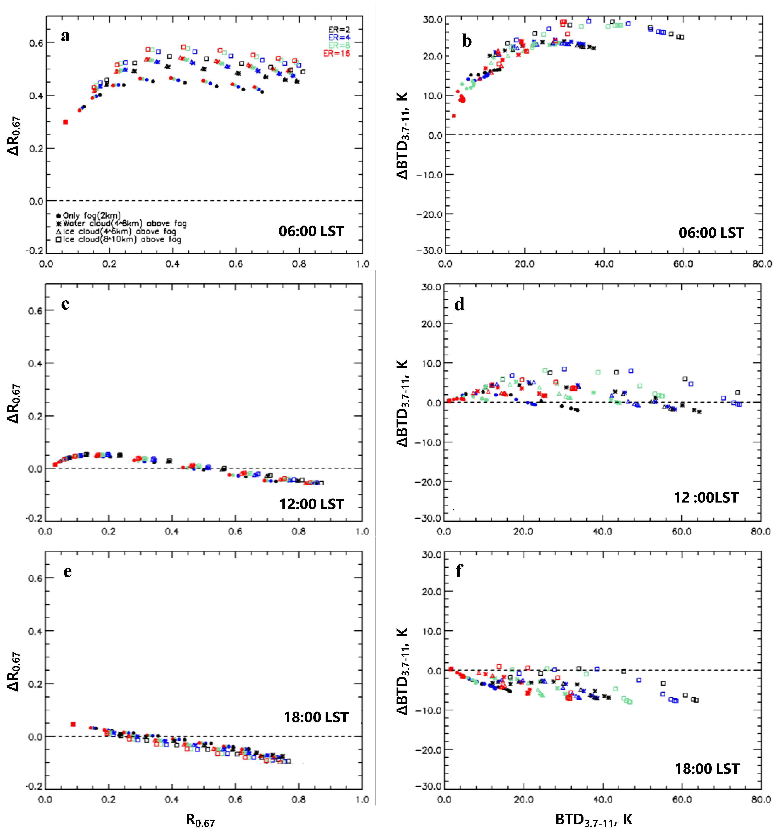
3.1. RTM Simulation for LSF

The simulation gives insight for fog detection at dawn, utilizing the three thresholds (ΔR_0.67, R_0.67, and ΔBTD_3.7-11) from the dual satellite observations (Figure 5). The optical characteristics of LSF can be estimated by both their simulations and observations. Since direct and diffuse radiation varies with the diurnal variation of SZA [36], the simulated ΔR_0.67 was largest at dawn (06:00 local standard time; LST). These significantly large differences (ΔR_0.67 or ΔBTD_3.7-11) can be used as indicators for LSF detection (Figure 5a,b). They are greater at dawn than at the other time ranges, due to the angle difference between the two satellites, compared to the spectral response function (SRF) [8].

The four colors (red, green, blue, and black) and four symbols (circle, asterisk, triangle, and rectangle) in Figure 5 denote the effective radii (ER: 2, 4, 8, 16 μm) and heights (FH or CH: 2, 4-6, 8-10 km) of the fog and cloud particles, respectively. RTM details are given in Table A4. The figures on the left show the relationship between ΔR_0.67 and R_0.67 at dawn, noon, and dusk (Figure 5a,c,e). The relationship between ΔBTD_3.7-11 and BTD_3.7-11 is presented on the right (Figure 5b,d,f). The ΔR_0.67 and ΔBTD_3.7-11 values from the dual-satellite relationship at dawn are about three times as large as those at noon and dusk, regardless of the various input conditions (e.g., high clouds above the fog layer, effective radii of fog or cloud, and their phase). In other words, the values at dawn under the LSF conditions (see also Figure A1 for the LSF definition) are substantially large compared to those at noon and dusk. However, there is a significant difference in seasonal variation between ΔR_0.67 and ΔBTD_3.7-11 (later shown in Figure 11).

While the ΔR_0.67 value at a given location was largest in the summer, the ΔBTD_3.7-11 was less sensitive to seasonality, and it was possibly useful for the other seasons (e.g., spring). The simulation implies that the dual satellite-derived thresholds for LSF sensing near the Korean Peninsula are best at dawn (Figure 5a,b) and worst at noon (Figure 5c,d). The values of ΔR_0.67 and ΔBTD_3.7-11 at dusk were relatively small and opposite to each other, compared to their values at dawn (Figure 5e,f). The relationship between ΔBTD_3.7-11 and BTD_3.7-11 is similar to that of ΔR_0.67 and R_0.67, except at noon. Fog detection in the former relationship was less useful than in the latter, because their variations with LSF height and ER were less systematic and included more detection uncertainties. Since the simulated differences (ΔR_0.67 and ΔBTD_3.7-11) at dawn were remarkably larger in the LSF situations than when the sky was clear, they can provide good thresholds for LSF detection from the dual-satellite observations.

The simulated ΔR_0.67 values near the Korean Peninsula at dawn need to be larger than 0.35, to separate the weather phenomena of LSF and clear-sky (Figure 5). Since the values under the LSF condition at dusk and noon did not generally reach the threshold, these dual-satellite observations were less useful. These results were caused by the angles made by the sun and the satellites in the space (i.e., SZA and RAA), which affect direct and diffuse radiation in radiative transfer. For these reasons, the dual-satellite relationship focused only on detection at dawn.

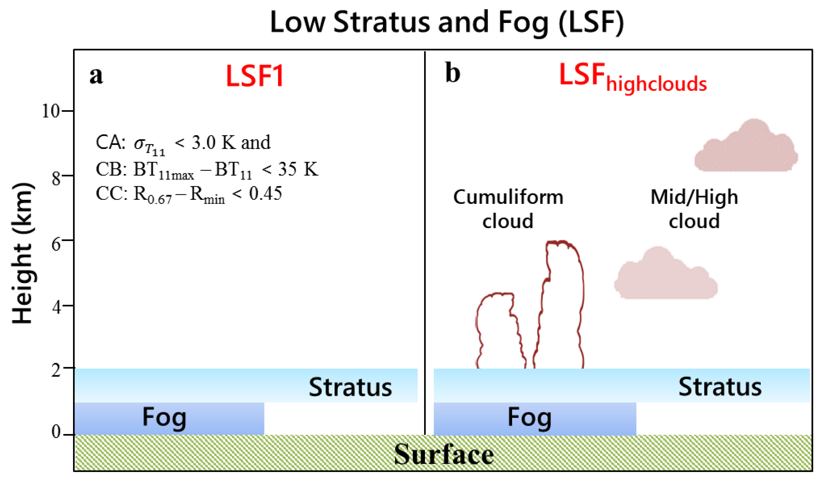
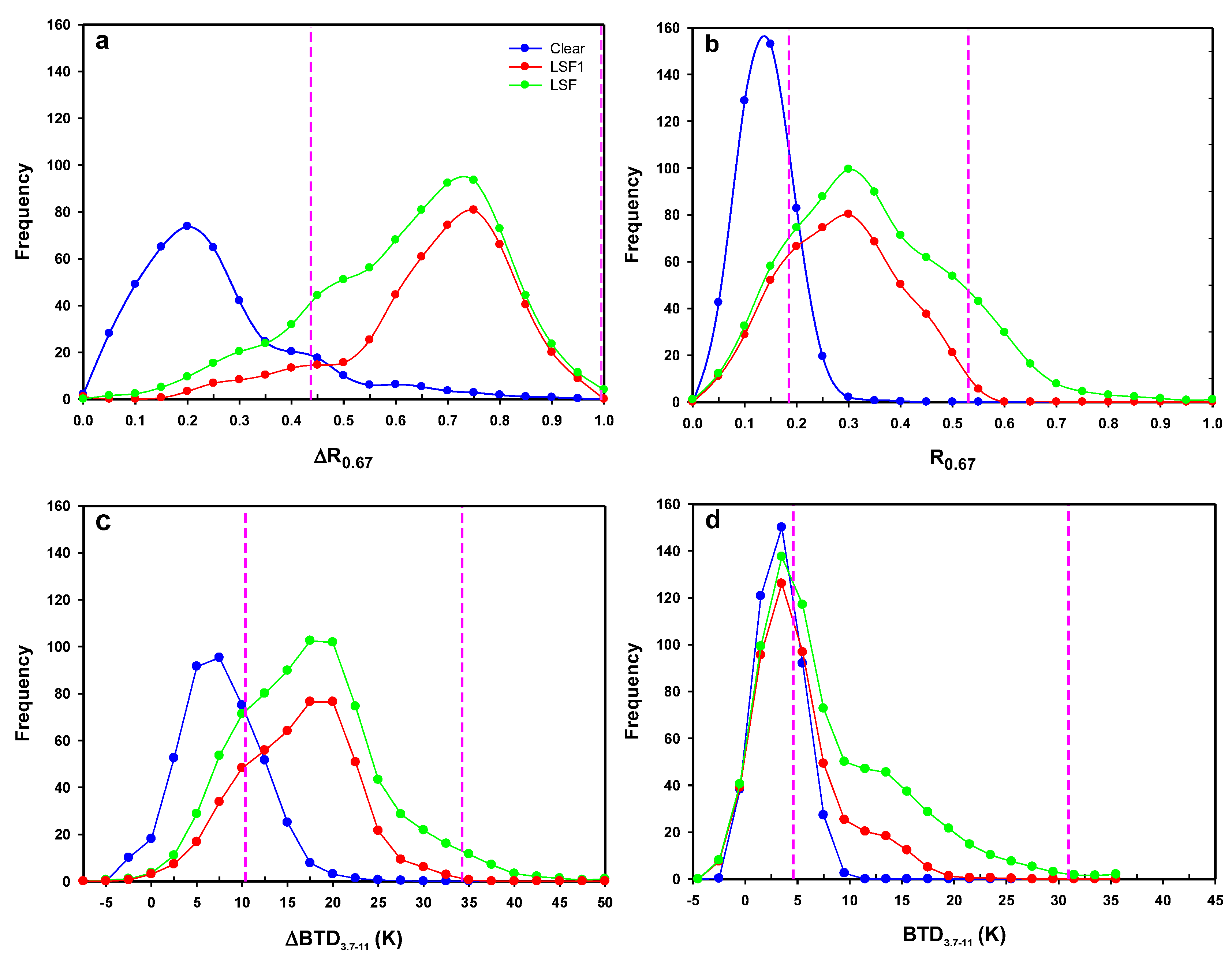
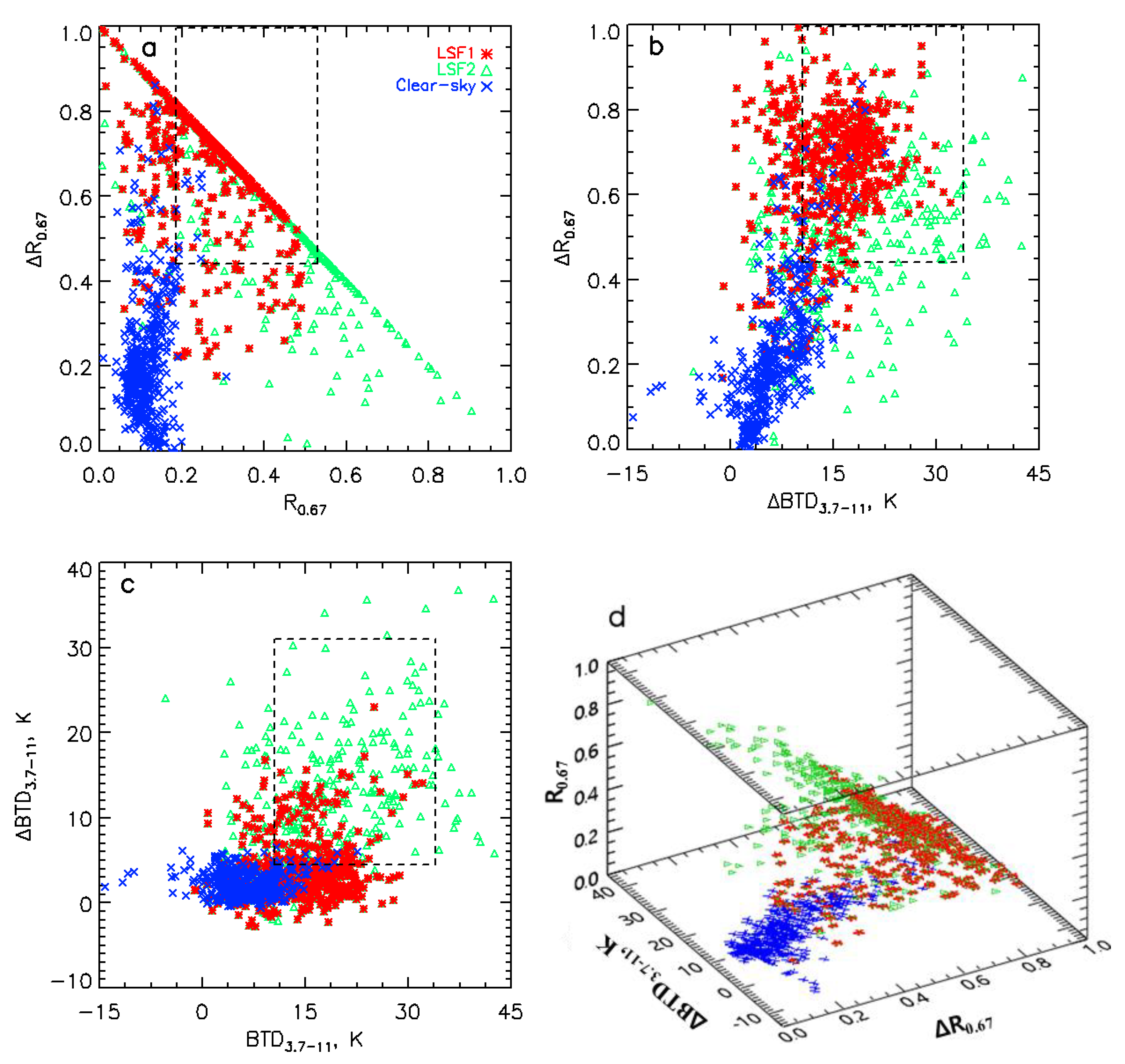
3.2. Optimum Thresholds for LSF Detection

In satellite-based LSF detection, the optimum thresholds are important for distinctly separating the clear-sky and LSF phenomena. After co-locating the ground-based and dual-satellite observations, the satellite data related to these weather phenomena (754 fog and 433 clear-sky occurrences) were collected in terms of reflectance (R_0.67 and ΔR_0.67) and brightness temperature (BTD_3.7-11 and ΔBTD_3.7-11) for each grid. To determine the optimum LSF thresholds for the variables ΔR_0.67, R_0.67, ΔBTD_3.7-11, and BTD_3.7-11, the frequency distributions of LSF (green), LSF1 (red), and clear-sky (blue) were presented, respectively (Figure 6). Here, LSF means total LSF (LSF1 and LSF_highclouds). The dashed lines in pink indicate the upper and lower thresholds between total LSF and clear-sky. There is no overlap with clear-sky in the upper-limit condition. However, it is necessary to filter the optically thick convective clouds without accompanying LSF (e.g., Yoo et al. [22]). The individual threshold was obtained iteratively until its total LSF POD reached a maximum under the limiting condition FAR ≤ 0.15, as shown in Table 4. This limitation is needed for the practical purpose of LSF detection. The POD maxima for the thresholds of the variables in the detection of either the total LSF or LSF1 during the study period were estimated to be ΔR_0.67 (0.82–0.90) > ΔBTD_3.7-11 (0.73–0.74) > R_0.67 (0.70–0.73) > BTD_3.7-11 (0.33–0.51). This indicates that the ΔR_0.67 threshold was best for both the total LSF and LSF1 detection (Figure 6a), while the BTD_3.7-11 threshold was worst (Figure 6d).

Based on their frequency distributions, all of the thresholds (ΔR_0.67, ΔBTD_3.7-11, and R_0.67) except for BTD_3.7-11 were useful for LSF detection. This means that the LSF phenomena was reasonably well detected by using the dual satellite thresholds on the satellite-observed scene, where the LSF and clear-sky cases coexist. Thus, both of the satellite observation variables ΔR_0.67 and ΔBTD_3.7-11 are included in the PI formulation of this study, while only R_0.67 was utilized in previous studies. The higher clouds above the LSF1 layer had a large effect on LSF and clear-sky classification in the ΔR_0.67 domain (Figure 6a), compared to R_0.67 in Figure 6b. In other words, the LSF detection from the ΔR_0.67 threshold was more accurate in the LSF1 cases (red line) without the accompanying higher clouds, than for the total LSF (green line), which is composed of both LSF1 and LSF_highclouds. LSF_highclouds included the clouds above the LSF1 layer, which were a hindrance to the LSF detection [22]. The ΔBTD_3.7-11 threshold was less sensitive to the higher clouds than the ΔR_0.67 threshold (Figure 6a), showing similar patterns of LSF (green line) and LSF1 (red line). In summary, the accuracy of LSF detection by the satellite-derived thresholds was affected by the clouds, and the seasonal and diurnal variations of the satellite observations.

Statistical verification on total LSF and LSF1 was performed with respect to the six threshold variables, ΔR_0.67, R_0.67, R_KMA, ΔBTD_3.7-11, BTD_3.7-11, and BTD_KMA, and the verification used fog and clear-sky data at 45 ground stations in South Korea at dawn during the study period. Five skill indices [37,38] were used for statistical analysis: HSS (Heidke Skill Score), CSI (Critical Success Index), POD (Probability of Detection), PC (Percentage Correct), and FAR (False Alarm Ratio). Table 4 shows the verification in terms of the skill scores for Period 1 (2012–2013), Period 2 (2014–2015), and the entire time span (2012–2015). The data from Period 1 denote the control case, and the fog detection thresholds were developed from these satellite observations. The data from Period 2 are the experimental case applied to the threshold quality evaluation. Other than FAR, the higher the skill indices, the higher the detection efficiency; the lower the FAR, the higher the accuracy. The thresholds R_KMA and BTD_KMA, used for daytime (SZA ≤ 60°) fog detection in KMA [19], were included with the other four thresholds, to allow for a comparison among the available conventional thresholds.

Table 4 shows that the HSS values of the total LSF for the whole period were in a descending magnitude order of △R_0.67 (0.699) > R_0.67 (0.588) > △BTD_3.7-11 (0.585) > R_KMA (0.489) > BTD_3.7-11 (0.369) > BTD_KMA (0.104). This means that the ΔR_0.67 threshold was the most effective at detecting fog at dawn. In addition, ΔR_0.67 and ΔBTD_3.7-11 (the dual satellite-observations) were at least 6–21% more accurate than the conventional COMS-only R_KMA or BTD_KMA thresholds [19]. The POD skill scores descend in the order of ΔR_0.67 > ΔBTD_3.7-11 > R_0.67 > R_KMA > BTD_3.7-11 > BTD_KMA. The results for Period 2 were similar to those for Period 1 (Figure 7a,b and Table 4), although, due to interannual variations, the scores were somewhat higher for the experimental data than those for the control. Compared to KMA [19], the ΔR_0.67 and ΔBTD_3.7-11 thresholds were excellent detection indicators overall.

The accuracy of ΔR_0.67 and R_0.67 in LSF1 was higher by 9–11% compared to the total LSF (Table 4). This indicates that the higher clouds above the LSF1 layer resulted in a significant hindrance to the detection by the reflectance thresholds. The LSF1 scores from the reflectance-based thresholds (i.e., ΔR_0.67, R_0.67, and R_KMA) were higher than for total LSF, suggesting that they were more sensitive to the clouds than to the brightness temperatures (ΔBTD_3.7-11, BTD_3.7-11, and BTD_KMA). The BTD-based thresholds did not show significant improvements over the LSF1, compared to the total LSF, probably due to their low sensitivities to the clouds.

Scatter diagrams in two dimensions (2D) and three dimensions (3D) were presented by using the top three thresholds of the variables (ΔR_0.67, ΔBTD_3.7-11 and R_0.67) in the POD scores (Table 4 and Figure 7 and Figure 8). In total, the cases of 473 LSF1 (red asterisk), 281 LSF_highclouds (green triangle), and 433 clear-sky (blue cross) were used. The LSF1 and LSF_highclouds cases are shown for Period 1 and Period 2, respectively, in

Table A5. Number of LSF cases that are used to develop and validate the optimum thresholds at the beginning of this study. The LSF1 and LSF_highclouds cases are shown for Period 1 and Period 2, respectively. The values in parentheses indicate the ratios (%) of the corresponding LSF types to the whole cases. Since the thresholds are not sensitive to the periods (i.e., interannual variation), the whole-period threshold values have been used in this study.

Period	LSF	LSF1	LSFhighclouds
Period 1 (2012–2013)	470 (100%)	296 (63%)	174 (37%)
Period 2 (2014–2015)	284 (100%)	177 (62%)	107 (38%)

. The ratio values of LSF1 to total LSF case are 62–63% for the two periods. The dashed-line boundaries in the 2D figures indicate the threshold values of the coordinate variables (Figure 8a–c). If the satellite observations in a grid that were co-located with the ground observed fog occurrences within their threshold boundaries, the LSF detection was regarded as a ‘success.’ LSF and clear-sky separation in the ΔR_0.67 versus R_0.67 diagrams (Figure 8a) and ΔR_0.67 versus ΔBTD_3.7-11 diagrams (Figure 8b) were excellent.

The LSF detection value of R_0.67 (69.6%) was obtained from 525 LSF cases out of 754 fog occurrences. The LSF1 detection value (73.2%) was obtained from 346 LSF1 cases out of 473 fog occurrences. Also, the POD scores of the ΔR_0.67 threshold in the ordinate were 81.6% for the total LSF, and 90.1% for LSF1, respectively. ΔR_0.67 from the dual satellite observations was 12.0–16.9% better at detecting the total LSF and LSF1 than the R_0.67 from the single COMS observations. The POD values of ΔR_0.67 compared to R_0.67 were enhanced by 12.0% for the total LSF and by 16.9% for LSF1. In other words, the ΔR_0.67 threshold was more accurate for LSF1 in the absence of higher clouds. In Figure 7b and Table 3, the POD values of ΔBTD_3.7-11 were 73.1–74.2% for the total LSF and LSF1, and somewhat higher than those of R_0.67 (69.6–73.2%). However, the FAR values of ΔBTD_3.7-11, 7.2–10.9%, were higher by 4–5% than those of R_0.67 (3.9–5.7%). Among the top three thresholds, ΔR_0.67 was the best indicator of LSF detection; the others were close.

Discrimination between the clear-sky and LSF cases at the BTD_3.7-11 axis (Figure 8c) was worse than for ΔR_0.67, R_0.67, or ΔBTD_3.7-11. This discrimination can be better seen in the 3D relationship depicted in Figure 8d. The LSF1, LSF_highclouds, and clear-sky weather phenomena were more distinguishable in the 3D depictions than in the 2D ones (Figure 8a,b). The thresholds derived from the three variables inherently had their own merits in the distinction of either LSF1 or LSF_highclouds from clear-sky phenomena, as follows; ΔR_0.67 (LSF1 from clear-sky), R_0.67 (LSF_highclouds from clear-sky), and ΔBTD_3.7-11 (the mixed feature of ΔR_0.67 and R_0.67). Rather than just using the two variables (ΔR_0.67 and R_0.67) proposed in Yoo et al. [8], this study used the top three variables for LSF detection.

We conducted a case study on fog occurrence at the island of Ulleungdo (130.9° E, 37.48° N; orange circles) at 06:15 LST on 17 April 2014, to estimate the optical properties of LSF in the 2D and 3D coordinates. These estimations were made using both the dual satellite observations and the RTM simulation (Figure 9). Regardless of the weather, the dual satellite observations (ΔR_0.67 and ΔBTD_3.7-11) are shown in grey circles in the background of Figure 9a–c. The R_0.67 and BTD_3.7-11 values were observed by using COMS data. Fog (orange circles) is also denoted in the 3D simulation (Figure 9d). According to ground-based reports at 06:00 LST, there were typical fog conditions (surface temperature = 11 °C, air temperature = 10.3 °C, humidity = 93% and visibility = 300 m). The fog type was classified as LSF1, based on this study’s higher cloud criteria (i.e., CA, CB, and CC). The ground-based observations also reported meteorological conditions that were consistent with the higher cloud estimation calculated from the satellite-derived criteria (total cloud amount = 10, amount of low and middle clouds = 10, and ceiling = 300 m). The cloud amount is scaled from 0 to 10.

The optical fog features at the island were investigated by simulating (Table A4) a) ∆R_0.67 versus R_0.67, b) ΔR_0.67 versus ΔBTD_3.7-11, and c) ΔBTD_3.7-11 versus R_0.67 (Figure 9a–c). The symbols and colors represent various fog or cloud conditions: i) just a fog layer (black for 0–1 km and sky-blue for 0–2 km), ii) fog with mid-level (4–6 km) clouds of different phases (red for water, blue for ice), and iii) fog with high-level (8–10 km) clouds (green). Clear-sky is denoted by pink. Similarly to Figure 8, the satellite observations inside the dashed-line rectangle were within the LSF detection threshold ranges for the same spatiotemporal conditions as for fog.

Figure 9a–c show that the higher cloud effect above the fog layer (i.e., the difference between LSF1 and LSF_highclouds) varied systematically with cloud height inside the dashed-line threshold rectangle. This was derived from any two of the three variables, ΔR_0.67, R_0.67, and ΔBTD_3.7-11. The simulated results of the middle clouds (blue for ice and red for water) showed they were mixed with each other, and difficult to separate. The simulated optical information, estimated from individual variables, did not necessarily agree with the estimates from the other variable, indicating that it was not unique. Overall, the RTM simulation (asterisks) for the case study agreed with the satellite-based observations (grey circles) and the ground-based fog observations (yellow).

The 2D simulations for the case study used the optical characteristics of the top three LSF detection variables. The actual fog case (orange circles) in the 3D simulation (Figure 9d) demonstrated three kinds of LSF optical features: i) a 1 km-height fog layer (i.e., LSF1) for ΔR_0.67 versus R_0.67 (Figure 9a), ii) a 2 km-height fog layer (i.e., LSF1) for ΔR_0.67 versus ΔBTD_3.7-11 (Figure 9b), and iii) fog (i.e., LSF_highclouds) with water-phase middle (4–6 km) clouds for ΔBTD_3.7-11 vs R_0.67 (Figure 9c). The clear-sky is shown as a pink circle in Figure 9d. The LSF1 estimation for ΔR_0.67 vs R_0.67 (Figure 9a) was the most reliable, based on the top two POD scores (Table 4), though the simulated fog information from each relationship, in terms of the LSF types was not unique (Figure 9).

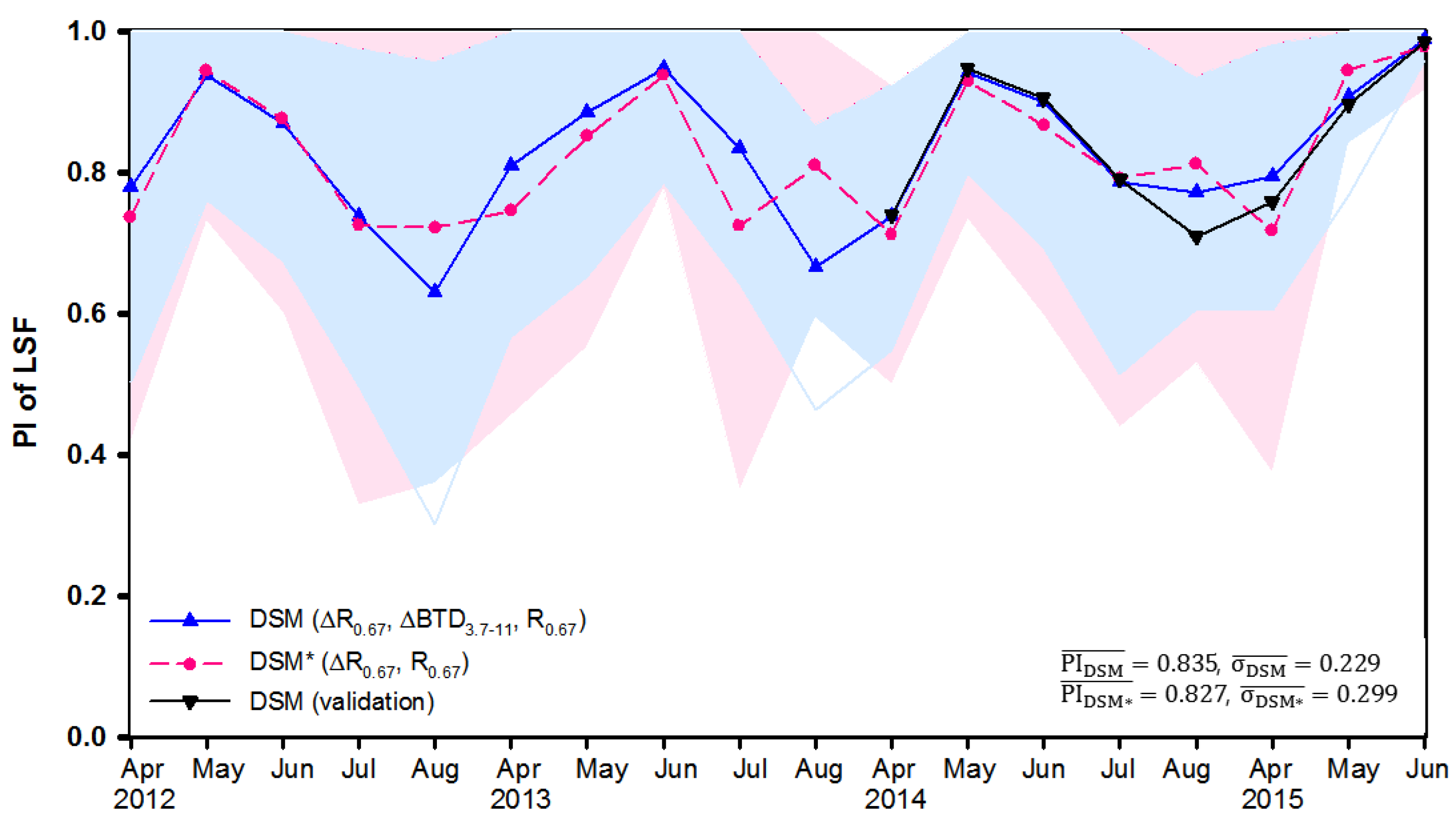
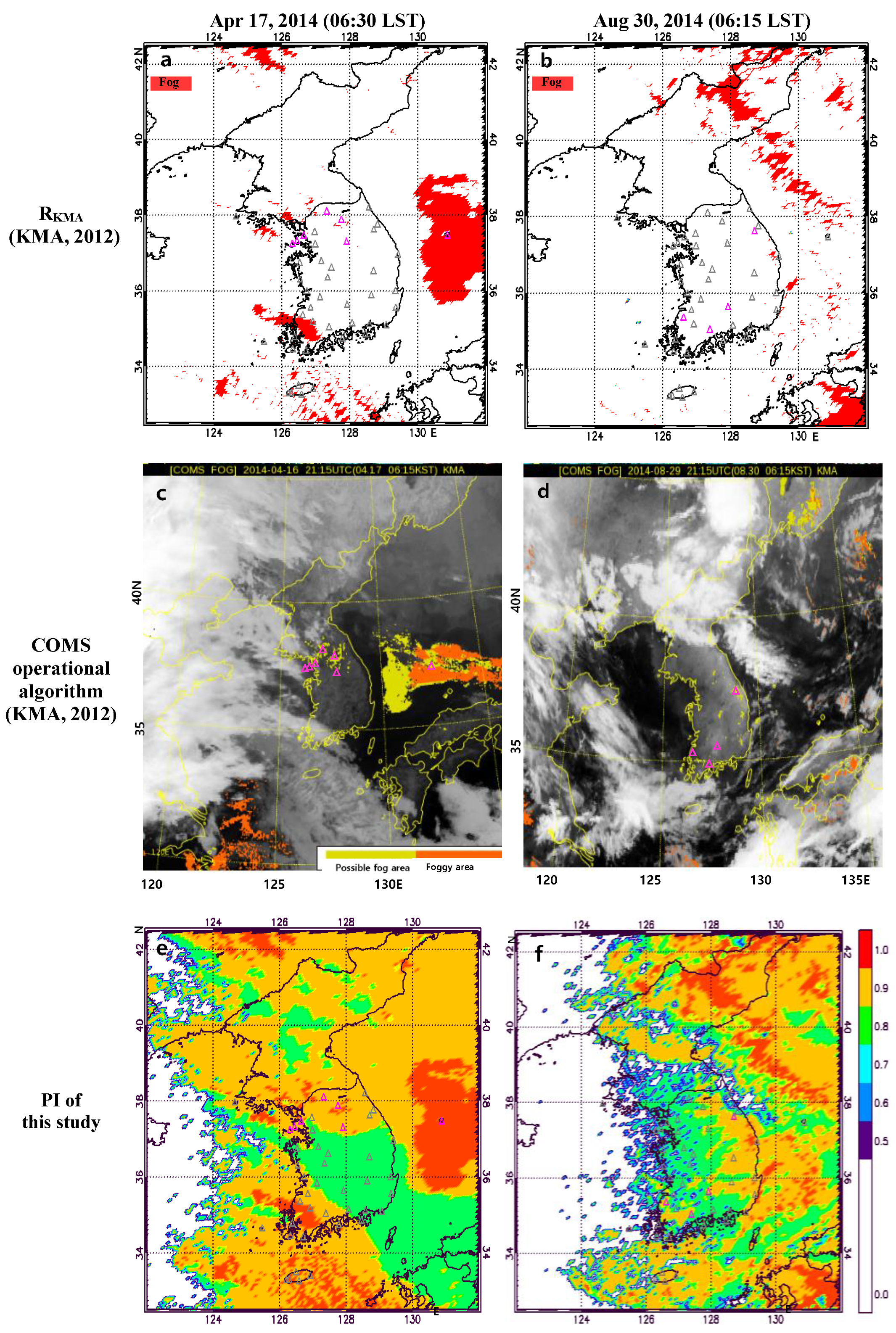
3.3. Probability Index for Improved LSF Detection

For validation, the PI method derived from the control data of the total LSF for Period 1 was applied to the experimental data for Period 2. We compared two methods: DSM* PI, using two variables (ΔR_0.67 and R_0.67) versus DSM PI, based on three variables (ΔR_0.67, ΔBTD_3.7-11, and R_0.67). The FAR value (13.5%) of DSM PI was relatively high, compared to those of other variables (4–9%) in

Table 5. POD values (ΔR_0.67, ΔBTD_3.7-11, and R_0.67), and the PI^est values of DSM and DSM* for the LSF detection validation during Period 2 (2014-2015) using the thresholds of the satellite-observed variables for Period 1 (2012–2013). The FAR values of the five methods are also given. **The ΔR_0.67 values within $\pm$2% have been used as the upper limit condition of PI^est. The POD values of DSM and DSM* have been obtained from the NFL data, not from $\mathrm{WF}\left({\mathrm{Class}}_{\mathrm{i}}\right)$.

	POD	PIest	FAR
ΔR0.67	**0.873		0.085
ΔBTD3.7-11	0.704		0.057
R0.67	0.715		0.043
DSM	0.982	0.853	0.135
DSM*	0.947	0.871	0.146

. However, the value seems to be acceptable in view of the results from previous studies (FAR ≤ ~15%) [4,39]. In addition, the POD values of DSM and DSM* were 0.982 and 0.947, respectively. Monthly average time series for the PODs of three thresholds (ΔR_0.67, R_KMA, and BTD_KMA) were investigated in terms of the monthly average for the 18 months between April 2012 and June 2015 (Figure 10). The number of fog occurrences per month varied from 17 to 75 for the period. The 18-month average values of the PODs were ΔR_0.67 (0.81), R_KMA (0.55), and BTD_KMA (0.14). The accuracy of the LSF detection was estimated in the order of ΔR_0.67 POD > R_KMA POD > BTD_KMA POD.

In Figure 11, DSM PI derived from three variables (ΔR_0.67, ΔBTD_3.7-11, and R_0.67) tends to be less variability within a month or season than DSM* PI. For reference, three WF values (1.0, 0.8, 0.6) have been used for DSM* PI, although the details about DSM* PI are beyond the scope of this study. The difference between DSM PI and DSM* PI was clear in the variability (one standard deviation) of the LSF detection accuracy, indicating that ΔBTD_3.7-11 resulted in less variability. The LSF detection variability of DSM PI was 23–25% less than that of DSM* PI. Although ΔR_0.67 was utilized as one of the three components in the PI calculation, it has a more seasonal dependence in the detection than the PI, showing the lowest POD in April 2014. The DSM PI, however, derived from both the reflectance and brightness temperatures, was less influenced by seasonality than the ΔR_0.67 threshold. This tendency was clear in April, showing that the averages of DSM PI and POD of ΔR_0.67 were 0.776 and 0.597, respectively (Figure 10 and Figure 11). This resulted from the low sensitivity of ΔBTD_3.7-11 to the seasonality, compared to ΔR_0.67. In summary, compared to an individual threshold, the PI was useful for LSF detection because of its high skill level, and the low seasonality and variability in the detection accuracy.

For the validation, the thresholds of three satellite-observed variables for Period 1 have been applied to the PI derivation for Period 2 (Figure 11). The optimum thresholds for Period 1 were 0.40 < ΔR_0.67 < 0.995, 12.0 K < ΔBTD_3.7-11 < 34.0 K, and 0.20 < R_0.67 < 0.55. Note that the thresholds in Table 4 were derived from the whole period (2012–2015) data. A monthly time series of DSM PI in Period 2 (black solid line) was approximately similar to that of DSM PI (blue solid line), derived from the whole-period thresholds. The PI average and the FAR values in Period 2 were 0.853 and 0.135, respectively (Table 5).

The DSM PI was applied to two cases of fog occurrences, to analyze its usefulness for monitoring LSF on 2D maps (Figure 12). The PI in the LSF spatial distribution can provide more specified probability values than 2–3 steps of KMA [19]. The two cases where there were at least four fog occurrences, based on ground observations, occurred at springtime and summertime dawn in 2014, one at 06:30 LST on April 17, and the other at 06:15 LST on August 30. Fog detection on the map was presented in two stages, fog and no fog, in the R_KMA threshold (Figure 12a,b); three stages, fog, possible fog, and no fog, in the KMA COMS operational algorithm [19,23] (Figure 12c,d); and with the seven PI values (no fog, 50%, 60%, 70%, 80%, 90%, and 100%) of this study (Figure 12e,f). These threshold values of KMA [19] were not accurate for actual fog cases [23], because they incorrectly detected fog areas as cloud-contamination pixels, and underestimated fog occurrence.

The figures in the left column of Figure 12 were used to investigate the fog-detection accuracy of the thresholds, and PI for seven fog occurrences at springtime dawn. The foggy stations in Figure 12a are denoted as pink triangles (see also Figure 2 and Table A2). The station numbers in South Korea are the west coast (2, 3, and 29), inland (25, 26, and 31), and the island of Ulleungdo (24). The R_KMA threshold failed fog detection in all of the stations except on the island (Figure 12a). In the COMS operational algorithm [19], three fog occurrences at the inland sites were classified as ‘possible fog,’ and only the fog event on Ulleungdo island was detected. The algorithm was unsuccessful at the west coast’s three stations. Two international airports, station 29 at Gimpo and station 3 at Incheon, are located in the region, and accurate fog monitoring is required for aviation. Most of the fog occurrences were successfully detected by the PI. The LSF possibility value was 100% at Ulleungdo, and it was 80% at the other six stations (Figure 12e). The PI was substantially better at springtime fog detection than the threshold for either R_KMA or the operational algorithm.

The fog-detection case at summertime dawn is presented in the right-hand column of Figure 12, which also shows four fog occurrences at ground stations 10, 27, 38, and 45. While none of the fog occurrences were detected by the R_KMA threshold or the COMS operational algorithm (Figure 12b,d), the PI was generally successful in the detection. The PI values were 0.9, except at ground station 45 (Sunchon), where it was a relatively value low (0.6) (Figure 12f). The four-station PI detection average (0.83) was remarkably high, in contrast with the detection failures of both the R_KMA and the operational algorithms. In both of the above case studies, the DSM PI was able to detect fog and determine its spatial distribution better than the KMA [19] single GEO of COMS threshold and algorithm methods.

4. Discussion

The previous study [8] that emphasized ΔR_0.67 was limited to the LSF detection in summer only. Based on the dual satellite method proposed in Yoo et al. [8], this study has attempted to extend the study period to spring and summer, and to develop the probability index (PI) of LSF utilizing ΔR_0.67 with additional satellite-observed variables, ΔBTD_3.7-11 and R_0.67. Compared to the threshold test (e.g., either fog or no fog) in Yoo et al. [8], PI in this study can visualize the LSF possibility into seven stages, and provides the practical application to LSF detection in its spatial distribution.

Table 6. Differences in the LSF detection between this study and Yoo et al. [8].

	This Study	Yoo et al. [8]
Theoretical basis	Dual satellite observations	Dual satellite observations
Season	Warm season (April to August)	Summer (June to August)
Variables used for LSF detection	ΔR0.67, ΔBTD3.7-11 and R0.67	ΔR0.67 and suggests R0.67
Detection method	Probability Index derived from three variables (ΔR0.67, ΔBTD3.7-11, and R0.67)	Threshold test of ΔR0.67 in the domain (ΔR0.67 vs R0.67)
LSF spatial distribution	Yes	No
Number of LSF probability classes	7	2 or 3
Variability in LSF detection accuracy in a month or season	Low	High

summarizes the differences between the two studies; the study period, the satellite variables for LSF detection, LSF probability classes, LSF spatial distribution, and the variability in the LSF detection accuracy for a month or season. The differences between this study and Yoo et al. [8] have been summarized in Table 6.

Using the dual satellite method (DSM), we have derived the probability index (PI) of low stratus and fog (LSF) from 18-month satellite and ground-based observations near the Korean Peninsula at dawn during the warm season. More climatological database values may help to provide more accurate PIs. The LSF retrieval was most effective in summer, based on the BRDF values of Yoo et al. [8]. We were able to extend the previous study period from June–August (summer) to the April-–August (warm season) by deriving PI from additional satellite-observed variables (△BTD_3.7-11 and R_0.67) to △R_0.67, as recommended by Yoo et al. [8]. The △BTD_3.7-11 test tends to reduce the variability of LSF PI accuracy in a month or season, but to raise the FAR to some extent. Overall, the LSF detection methods of DSM PI, DSM* PI and ΔR_0.67 are found to have their own merits of LSF detection skill in view of POD, FAR, and favorable seasons, etc. Also, the dual satellite-observed methods may be selectively utilized for an operational purpose, for instance, considering seasons of LSF occurrence seasons and the acceptable FAR limit.

Thus, the current LSF PI retrieval algorithm is expected to be less useful for non-warm seasons and at dusk, and this may need to be investigated in future studies. The validation for DSM PI has was carried out using at 45 ground stations in South Korea, including some island stations. However, the validation was not performed over the open sea, due to the lack of these stations. Two case studies have been selected to validate DSM PI, but the LSF signals over the sea (Figure 12e,f) needs to be verified in the future for whether they were fog or low stratus, and furthermore, LSF1 or LSF_highclouds. Although PI values in the case of middle/high clouds without fog have not been investigated in this study, the clouds are expected to lower the PI value, based on the LSF_highclouds values out of thresholds. In addition, the visibility meter data may be utilized, particularly in the coastline. Also, there may be a case study limitation to some degree.

5. Conclusions

A new method for LSF detection, called DSM, was developed in terms of the LSF probability index (PI) determined from the nearly simultaneous observations of dual geostationary-orbit satellites (COMS and FY-2D) and ground station observations during the warm season of 18 months. The ground-based observations yielded 754 fog and 433 clear-sky occurrences that were utilized to validate the satellite-observed LSF detection. An RTM simulation demonstrated that LSF detection and optical properties were generally consistent with the dual-satellite observations. The POD values of six detection thresholds were ranked in a descending order of magnitude: △R_0.67 > △BTD_3.7-11 > R_0.67 > R_KMA > BTD_3.7-11 > BTD_KMA. The DSM PI was derived from a combination of observations (ΔR_0.67 and ΔBTD_3.7-11 from the dual satellites; R_0.67 from a single GEO of COMS) in association with the top three POD scores for detection probability. The PI accuracy was analyzed with respect to the fog detection rates of the conventional thresholds (R_KMA and BTD_KMA) and the KMA [19] operational algorithm from COMS.

Two case studies using maps of spatial fog distribution at springtime and summertime dawn addressed the PI’s improved method of fog detection. Compared to the conventional methods of KMA [19] and single threshold (ΔR_0.67; [8]), the PI has three merits: i) a high LSF detection rate, ii) more specified (seven classes) LSF spatial distribution, and iii) variability of the detection accuracy in a month or season. The △BTD_3.7-11 component in PI was found to lead to the trend of low variability, based on the comparison of the DSM PI with the DSM* PI, which was derived from the two reflectance variables (△R_0.67 and R_0.67) The PI has timely implications for LSF detection, because the newly available satellite-based observations from the advanced GEOs (e.g., GK-2A launched on December 5, 2018 [40]; FY-4A [41] and Himawari-8 [42]) have additional multi-channels with higher spatiotemporal resolution than do previous satellites. The DSM technique can be applied to other meteorological/environmental variables (e.g., cloud and dust) and satellite calibration, as well as near real-time LSF monitoring.

References

1. Ahrens, C.D. An Introduction to Weather, Climate, and the Environment, 8th ed.; Brooks/Cole: Belmont, CA, USA, 2007; p. 23. [Google Scholar]
2. Egli, S.; Thies, B.; Bendix, J. A hybrid approach for fog retrieval based on a combination of satellite and ground truth data. Remote Sens. 2018, 10, 628. [Google Scholar] [CrossRef]
3. Cermak, J.; Eastman, R.M.; Bendix, J.; Warren, S.G. European climatology of fog and low stratus based on geostationary satellite observations. Q. J. R. Meteorol. Soc. 2009, 135, 2125–2130. [Google Scholar] [CrossRef]
4. Chaurasia, S.; Sathiyamoorthy, V.; Paul Shukla, B.; Simon, B.; Joshi, P.C.; Pal, P.K. Night time fog detection using MODIS data over northern India. Meteor. Appl. 2011, 18, 483–494. [Google Scholar] [CrossRef]
5. Zhang, S.; Yi, L. A comprehensive dynamic threshold algorithm for daytime sea fog retrieval over the Chinese adjacent seas. Pure Appl. Geophys. 2013, 170, 1931–1944. [Google Scholar] [CrossRef]
6. Cermak, J.; Bendix, J. Dynamical nighttime fog/low stratus detection based on Meteosat SEVIRI data: A feasibility study. Pure Appl. Geophys. 2007, 164, 1179–1192. [Google Scholar] [CrossRef]
7. Ellord, G.P.; Gultepe, I. Inferring low cloud base heights at night for aviation using satellite infrared and surface temperature. Pure Appl. Geophys. 2007, 164, 1193–1205. [Google Scholar] [CrossRef]
8. Yoo, J.M.; Choo, G.H.; Lee, K.H.; Wu, D.L.; Yang, J.H.; Park, J.D.; Choi, Y.S.; Shin, D.B.; Jeong, J.H.; Yoo., J.M. Improved detection of low stratus and fog at dawn from dual geostationary (COMS and FY–2D) satellites. Remote Sens. Environ. 2018, 211, 292–306. [Google Scholar] [CrossRef]
9. Andersen, H.; Cermak, J.; Solodovnik, I.; Lelli, L.; Vogt, R. Spatiotemporal dynamics of fog and low clouds in the Namib unveiled with ground and space-based observations. Atmos. Chem. Phys. Discuss 2018. [Google Scholar] [CrossRef]
10. Egli, S.; Thies, B.; Drönner, J.; Cermak, J.; Bendix, J. A 10 year fog and low stratus climatology for Europe based on Meteosat Second Generation data. Q. J. R. Meteorol. Soc. 2017, 143, 530–541. [Google Scholar] [CrossRef]
11. Bendix, J. A satellite-based climatology of fog and low-level stratus in Germany and adjacent areas. Atmos. Res. 2002, 64, 3–18. [Google Scholar] [CrossRef]
12. Musial, J.; Hüsler, F.; Sütterlin, M.; Neuhaus, C.; Wunderle, S. Daytime low stratiform cloud detection on AVHRR imagery. Remote Sens. 2014, 6, 5124–5150. [Google Scholar] [CrossRef]
13. Cermak, J.; Bendix, J. A novel approach to fog/low stratus detection using meteosat 8 data. Atmos. Res. 2008, 87, 279–292. [Google Scholar] [CrossRef]
14. Eyre, J.R.; Brownscomve, J.L.; Allam, R.J. Detection of fog at night using advanced very high resolution radiometer (AVHRR) imagery. Meteorol. Mag. 1984, 113, 266–271. [Google Scholar]
15. Cermak, J.; Bendix, J. Fog/low stratus detection and discrimination using satellite data. In Proceedings of the COST722 Midterm Workshop on Short Range Forecasting Methods of Fog, Visibility and Low Clouds, Langen, Germany, 20 October 2005. [Google Scholar]
16. Gultepe, I.; Pagowski, M.; Reid, J. A satellite-based fog detection scheme using screen air temperature. Weather Forecast. 2007, 22, 444–456. [Google Scholar] [CrossRef]
17. Dybbroe, A. Automatic Detection of Fog at Night Using AVHRR Data. In Proceedings of the 6th AVHRR Data Users’ Meeting, Belgirate, Italy, 29 June–2 July 1993; pp. 245–252. [Google Scholar]
18. Ellord, G.P. Advances in the detection and analysis of fog at night using GOES multispectral infrared imagery. Weather Forecast. 1995, 10, 606–619. [Google Scholar] [CrossRef]
19. KMA, National Meteorological Satellite Center. Fog detection. In Algorithm Theoretical Basis Document, Fog-Version 1.0; KMA: Seoul, Korea, 2012. [Google Scholar]
20. Kim, S.H.; Suh, M.S.; Han, J.H. Development of fog detection algorithm during nighttime using Himawari-8/AHI satellite and ground observation data. Asia-Pac. J. Atmos. Sci. 2018. [Google Scholar] [CrossRef]
21. Shin, D.; Kim, J.H. A new application of unsupervised learning to nighttime sea fog detection. Asia-Pac. J. Atmos. Sci. 2018, 54, 527–544. [Google Scholar] [CrossRef]
22. Yoo, J.M.; Jeong, M.J.; Hur, Y.M.; Shin, D.B. Improved fog detection from satellite in the presence of clouds. Asia-Pac. J. Atmos. Sci. 2010, 46, 29–40. [Google Scholar] [CrossRef]
23. KMA, National Meteorological Satellite Center. Improving Retrieval Algorithm for Fog Detection Using COMS Observation Data; KMA: Seoul, Korea, 2015. [Google Scholar]
24. Lee, T.F.; Turk, F.J.; Richardson, K. Stratus and fog products using GOES-8-9 3.9-µm data. Weather Forecast. 1997, 12, 664–677. [Google Scholar] [CrossRef]
25. Turk, J.; Vivekanandan, J.; Lee, T.; Durkee, P.; Nielsen, K. Derivation and applications of near-infrared cloud reflectances from GOES-8 and GOES-9. Bull. Amer. Meteor. Soc. 1998, 37, 819–831. [Google Scholar]
26. Schreiner, A.J.; Ackerman, S.A.; Baum, B.A.; Heidinger, A.K. A multispectral technique for detecting low-level cloudiness near sunrise. J. Atmos. Ocean. Tec. 2007, 24, 1800–1810. [Google Scholar] [CrossRef]
27. Lee, J.; Chung, C.; Ou, M. Fog detection using geostationary satellite data: Temporally continuous algorithm. A. Pac. J. Atmos. Sci. 2011, 47, 113–122. [Google Scholar] [CrossRef]
28. Ishida, H.; Miura, K.; Matsuda, T.; Ogawara, K.; Goto, A.; Matsuura, K.; Sato, Y.; Nakajima, T.Y. Investigation of low-cloud characteristics using mesoscale numerical model data for improvement of fog-detection performance by satellite remote sensing. J. Appl. Meteorol. Climatol. 2014, 53, 2246–2263. [Google Scholar] [CrossRef]
29. National Meteorological Satellite Center of KMA. Available online: http://nmsc.kma.go.kr/html/homepage/ko/chollian/choll_img.do (accessed on 23 March 2019).
30. National Satellite Meteorological Center of CMA. Available online: http://www.nsmc.org.cn/en/NSMC/Contents/Instruments_VISSR-II.html (accessed on 23 March 2019).
31. Wu, X.; Li, S.; Liao, M.; Cao, Z.; Wang, L.; Zhu, J. Analyses of seasonal feature of sea fog over the Yellow Sea and Bohai Sea based on the recent 20 years of satellite remote sensing data. Haiyang Xuebao 2015, 37, 63–72. [Google Scholar]
32. data.kma.go.kr. Available online: https://data.kma.go.kr/data/grnd/selectAsosRltmList.do?pgmNo=36 (accessed on 23 March 2019).
33. data.kma.go.kr. Available online: https://data.kma.go.kr/data/rmt/rmtList.do?code=372&pgmNo=568 (accessed on 23 March 2019).
34. Ricchiazzi, P.; Yang, S.; Gautier, C.; Sowle, D. SBDART: A research and teaching software tool for plane-parallel radiative transfer in the Earth’s atmosphere. Bull. Amer. Meteor. Soc. 1998, 79, 2101–2114. [Google Scholar] [CrossRef]
35. Yoo, J.M.; Jeong, M.J.; Yun, M.Y. Optical properties of fog from satellite observation (MODIS) and numerical simulation. Asia-Pac. J. Atmos. Sci. 2006, 42, 291–305. [Google Scholar]
36. Liou, K.N. Radiation and Cloud Processes in the Atmosphere: Theory, Observations, and Modeling, Oxford Monographs on Geology and Geophysics No. 20; Oxford University Press: New York, NY, USA, 1992; pp. 104–105. [Google Scholar]
37. von Storch, H.; Zwiers, F.W. Statistical Analysis in Climate Research; Cambridge University Press: Cambridge, UK, 1999; 405p. [Google Scholar]
38. Cermak, J.; Bendix, J. Detecting ground fog from space–A microphysics-based approach. Int. J. Remote Sens. 2011, 32, 3345–3371. [Google Scholar] [CrossRef]
39. Chaurasia, S.; Gohil, B.S. Detection of day time fog over India using INSAT-3D data. IEEE J. Sel. Topics Appl. Earth Observ. Remote Sens. 2015, 8, 4524–4530. [Google Scholar] [CrossRef]
40. National Meteorological Satellite Center of KMA. Available online: http://nmsc.kma.go.kr/html/homepage/en/ver2/static/selectStaticPage.do?view=satellites.gk2a.gk2aIntro (accessed on 23 March 2019).
41. Yang, J.; Zhang, Z.; Wei, C.; Lu, F.; Guo, Q. Introducing the new generation of Chinese geostationary weather satellites, Fengyun-4. Bull. Amer. Meteor. Soc. 2017, 98, 1637–1658. [Google Scholar] [CrossRef]
42. Bessho, K.; Date, K.; Hayashi, M.; Ikeda, A.; Imai, T.; Inoue, H.; Kumagai, Y.; Miyakawa, T.; Murata, H.; Ohno, T.; et al. An introduction to Himawari-8/9-Japan’s new-generation geostationary meteorological satellites. J. Meteorol. Soc. Jpn. 2016, 94, 151–183. [Google Scholar] [CrossRef]
Figure 1. Viewing zenith angles (VZAs) of the two geostationary satellites (COMS and FY-2D) available for near-simultaneous observations of low stratus and fog (LSF) at dawn near the Korean Peninsula. The VZA difference between the satellites is 46.5° in Seoul.
Remotesensing 11 01283 g001
Figure 2. Locations of the 45 meteorological stations in South Korea used for the LSF analysis.
Remotesensing 11 01283 g002
Figure 3. (a) Seven classes from the combination of the three threshold tests using ΔR0.67, ΔBTD3.7-11, and R0.67 for the formulation of the LSF probability index (PI) in the dual-satellite method (DSM). (b) Normalized frequency distributions of the classes.
Remotesensing 11 01283 g003
Figure 4. Flow chart for LSF detection in South Korea at dawn during the warm season (April-August) between April 2012 and June 2015, based on near-simultaneous satellite observations from COMS and FY-2D. The values of NFL, PIest, Classi and WF(Classi) in a grid have been calculated from the long-term database (i.e., 18 months), while the values of Classobs and WF(Classobs) over the real-time scene are assigned to one among seven classes of Classi and WF(Classi), i = 1 to 7.
Remotesensing 11 01283 g004
Figure 5. Simulated results of ΔR0.67 vs R0.67 (a,c,e) and ΔBTD3.7-11 vs BTD3.7-11 (b,d,f) under the Radiative Transfer Model (RTM) conditions of Table A4. Each simulation on 18 July 2014 was shown in the dual-satellite relationship of FY-2D and COMS at three different times: 06:00 LST (for dawn), 12:00 LST (noon), and 18:00 LST (for dusk). The reflectance and BTD3.7-11 simulations are presented in the left- and right-hand columns, respectively. The clear-sky value is shown in the leftmost one (red square) in each figure.
Remotesensing 11 01283 g005
Figure 6. Frequency distributions of total LSF (green), LSF1 (red), and clear-sky (blue) with respect to (a) ΔR0.67, (b) R0.67, (c) ΔBTD3.7-11, and (d) BTD3.7-11. The pink dotted lines indicate the optimum threshold values that can be used for LSF detection when FAR ≤ 0.15. The ground-based observations of clear-sky and fog were used for the distributions, and the fog data were categorized into LSF1 and LSFhighclouds with the help of satellite-observed criteria. Total LSF means the summation of LSF1 and LSFhighclouds. Note that the upper limit (pink dotted line) is not needed to separate clear cases from fog, but is included to separate out optically thick convective clouds.
Remotesensing 11 01283 g006
Figure 7. Statistical verification with respect to six threshold components (ΔR0.67, ΔBTD3.7-11, R0.67, RKMA, BTD3.7-11, and BTDKMA) for Period 1 (control data period) and Period 2 (experimental data period) of (a) POD and (b) HSS. The six threshold values were verified by using ground observations from 754 fog and 433 clear-sky occurrences in South Korea.
Remotesensing 11 01283 g007
Figure 8. Scatter diagrams of satellite-observations. (a) ΔR0.67 vs R0.67, (b) ΔR0.67 vs ΔBTD3.7-11, (c) ΔBTD3.7-11 vs BTD3.7-11, and (d) the 3D plot of the three variables (ΔR0.67, ΔBTD3.7-11, and R0.67) from the ground observations of 754 fog and 433 clear-sky occurrences. The weather phenomena of LSF1, LSFhighclouds, and clear-sky are shown as red, green, and blue colors, respectively.
Remotesensing 11 01283 g008
Figure 9. RTM results near the Korean Peninsula (122–132° E, 32.5–42.5° N) during a fog period at Ulleungdo island (orange circles) at 06:15 LST on 17 April 2014. The simulation was performed without higher clouds (LSF1; black and sky-blue), with fog and middle-level/high-level clouds (LSFhighclouds; red, blue and green), and with clear sky (pink) in the domain of (a) ΔR0.67 vs R0.67, (b) ΔR0.67 vs ΔBTD3.7-11, and (c) ΔBTD3.7-11 vs R0.67. The 3D plot of the three variables (ΔR0.67, ΔBTD3.7-11, and R0.67) is shown in (d). The input conditions were the same as for the simulation of the four figures.
Remotesensing 11 01283 g009
Figure 10. Time series for the monthly fog-detection average values at dawn over South Korea (45 stations). The three series in the figure are shown for the PODs of (i) ΔR0.67 from the dual satellite observations (red rectangles), (ii) RKMA from COMS (blue triangles), and (iii) BTDKMA from COMS (green circles).
Remotesensing 11 01283 g010
Figure 11. Same as Figure 10 except for DSM PI (▲, blue solid line) and DSM* PI (●, pink dashed line) with one standard deviation ( ± 1 σ ) of PI values in a month. The shaded area in blue and pink indicate the standard deviation values of DSM PI and DSM* PI, respectively. The overbars of PI and σ indicate the averages of their 18 monthly values, respectively. In addition, a time series for DSM PI in Period 2 (▼, black solid line) was shown for validation.
Remotesensing 11 01283 g011
Figure 12. Spatial distributions of fog probabilities at dawn (06:30 LST) on 17 April 2014 near the Korean Peninsula from the three fog detection methods: (a) RKMA threshold [19], (c) the operational algorithm with a COMS image [19], and (e) the PI of this study. (b) As in Figure 12a, except for the date and time (06:15 LST on 30 August 2014). (d) Same as in Figure 12c, except for the date and time. (f) Same as in Figure 12e, except for the date and time. The white areas in Figure 12e,f mean ‘no fog’.
Remotesensing 11 01283 g012